The temporal and spatial variation of chlorophyll a concentration in the China Seas and its impact on marine fisheries

Highlights

1. Spatial and temporal variation of chlorophyll a concentration in China Seas over long time series and characteristics of chlorophyll a concentration at different time scales.

2. Autocorrelation test of chlorophyll a concentration in China Seas and temporal decomposition to study the periodicity of temporal variation of chlorophyll a concentration.

3. Analysis of the effects of multiple factors such as ocean surface temperature, seawater nutrients (phosphate, nitrate, silicate), partial pressure of CO₂, and physical movement of seawater on chlorophyll a concentration in China Seas, as well as a summative analysis considering the above factors.

4. To study the change of algal habitat and analyze the impact on the development of marine fishery, taking Zhoushan fishing grounds as an example, to draw the society’s attention to the sustainable development of marine fishery.

1 Introduction

Chlorophyll a is an important group of pigments associated with photosynthesis. Phytoplankton fix carbon dioxide through photosynthesis and absorb atmospheric carbon dioxide through a biochemical “biological pump” function and remit it to the ocean carbon pool (Falkowski et al., 2000). Therefore, chlorophyll a plays a very important role in the global ecosystem carbon cycle. In addition, chlorophyll a, as an important biological indicator of marine primary productivity (Dang et al., 2022), phytoplankton extant and some fishing grounds, can provide necessary basic support for the development of marine fisheries and also provide a restoration countermeasure for the increasingly depleted fishery resources (Cury et al., 2000). Therefore, it is very important to study the spatial and temporal characteristics of chlorophyll in the China Seas to explore the influence mechanism of marine pollution (e.g., red tide), early warning and exploitation of marine resources (Wang et al., 2022). In addition, chlorophyll a concentration reflects the environmental quality of water ecology and is an important parameter for evaluating the eutrophication status of seawater (Firdhouse et al, 2019), and the study of the influencing factors of chlorophyll a can effectively analyze the changes of marine chlorophyll concentration. Therefore, the spatial and temporal distribution of chlorophyll concentration and its correlation with environmental factors can reflect the regional marine ecological and environmental quality status, which has important research value.

With the rapid development of the application of remote sensing technology in the marine field, the use of satellite data to establish regression and inversion models of chlorophyll concentration to achieve the determination of chlorophyll concentration provides a possibility for real-time monitoring of a wide range of sea areas (Blondeau-Patissier et al., 2014). International research on the study of chlorophyll a is mainly focused on the following aspects. The establishment and validation of chlorophyll concentration inversion models based on remote sensing technology methods, such as the establishment of remote sensing methods for chlorophyll-a concentration inversion in semi-arid turbid waters (Lin et al., 2011), and the algorithm for chlorophyll-a concentration inversion in seawater with different nutrient status (Hu et al., 2012). It is concerned with the temporal and spatial characteristics of chlorophyll-a, the seasonal variation of chlorophyll-a (Gregg et al., 2003) and the response to climate change (Behrenfeld et al., 2005). The relationship between chlorophyll-a and marine ecosystems and the interaction of environmental factors have been studied, such as investigating the chlorophyll-a concentration and species composition of different phytoplankton communities (Fragoso et al., 2018) and exploring the effects of water temperature, nutrient concentration and light intensity on the spatial and temporal variation of chlorophyll-a (Demarcq et al., 2003). Chlorophyll-a monitoring and management: Using chlorophyll-a data for monitoring and management of marine ecosystems, such as detecting seawater eutrophication and mitigating marine pollution (Paerl, 2009).

Research in China has focused on the establishment and validation of chlorophyll concentration inversion models (Yue et al., 1999), the inversion of chlorophyll concentration models for different China Seas using the Gaofen 4 satellite (Yang et al., 2017), and the validation of simultaneous field sampling data for chlorophyll a concentration (Zheng et al., 2017). Some progress has also been made in the study of the spatial and temporal variation of chlorophyll in China Seas. Lian et al. (2020) studied the characteristics and causes of seasonal variation of surface chlorophyll a in the South China Sea and analyzed the effects of surface ocean temperature and dynamic processes on marine chlorophyll. Cong et al. (2006) studied the changes of chlorophyll a concentration in the Chinese continental shelf seas from 1998 to 2003 based on satellite inversion, and Hao (2010) studied the spatial and temporal distribution characteristics and environmental regulation mechanisms of chlorophyll a and primary productivity in Chinese coastal seas. In China, there are few analyses of the spatial and temporal variability of marine chlorophyll a concentration over long time series. And there is a lack of comparative variation analysis of the overall China Seas area and each constituent sea area. Moreover, the spatial and temporal variability of chlorophyll a concentration has not been explored regularly.

In this paper, we constructed a long time series of chlorophyll a concentration data in China Seas using the marine chlorophyll a concentration products of satellite remote sensing (MODIS/Aqua) inversions from 2002-2022. The temporal and spatial variation characteristics of chlorophyll a concentration were analyzed on the basis of long time-series of chlorophyll a concentration data, and the temporal coefficient of variation and spatial coefficient of variation were used to characterize the temporal fluctuations and spatial heterogeneity. Secondly, the accumulation difference was used to represent the cumulative multi-year variation of chlorophyll a concentration in China Seas. In addition, the correlation between chlorophyll a concentration and ocean surface temperature, ocean net primary productivity and seawater carbon dioxide partial pressure were analyzed to explore the influencing factors of chlorophyll a concentration in Chinese marine waters. Finally, the influence of the change of ocean chlorophyll a concentration on marine fishing grounds was analyzed using Zhoushan fishing grounds as an example. It is expected to provide some data support and research reference for China’s marine research and provide an important scientific basis for marine pollution management, marine ecological protection and rational marine use and development in China.

2 Study area, data and methods

2.1 Study area

Since this study requires the determination of specific chlorophyll a study values for specific sea areas, boundary delimitation has an impact on the study results. The boundary ranges of the four Chinese seas for this study are described (the specific boundary ranges may be subject to international law and controversy among related countries, and there are no strict sea boundary restrictions in this paper):

Boundary range of the Bohai Sea: East: bordered by the Yellow Sea. South: bordered by Shandong Peninsula. West: bordered by Hebei, Liaoning and other Chinese mainland provinces. North: Connected to the Gulf of Korea.

Boundary range of the Yellow Sea: East: bordering with North Korea, including Yeonpyeong Island, the Jinju Peninsula and other areas. South: bordered by the Bohai Sea. West: bordered by the Shandong Peninsula of China. North: Connected to the Democratic People’s Republic of Korea via Yalu River and East Korea Bay.

Boundary range of the East China Sea: East: bordered by Ryukyu Islands of Japan in the east. South: bordered by the Taiwan Strait. West: bordered by the Korea Strait. North: bordered by the Yellow Sea.

Boundary range of the South China Sea: East: bordered by Luzon Island of the Philippines. South: South to the Strait of Malacca. Southwest: bordering the Indonesian province of Papua, including the South China Sea Islands. West: bordered by Vietnam. North: Connected to the East China Sea.

2.2 Data source

2.2.1 Chlorophyll a concentration data

Chlorophyll a (Chl-a) concentration data were obtained from the NASA Oceancolor website (https://oceancolor.gsfc.nasa.gov/) Chlor_a L3B Chl-a data product obtained by the MODIS (MODerate resolution Imaging) sensor on board the Aqua satellite. The temporal resolution of the products used in this study is months, and the spatial resolution is 4 km, and the data used in this paper span the period from August 2002 to November 2022. The data product is based on the algorithm of Hu et al. (2012), which combines the empirical band-difference method at low Chl-a concentrations and the ratio-transformation method at higher Chl-a concentrations. Cui et al. (2014) verified the accuracy and applicability of Chl-a concentration inversion using this method for MODIS data in China Seas by comparing the MODIS satellite Oceancolor products with the measured values in the Yellow Sea and East China Sea. And the data error showed that the error was 32% in the Chinese near-shore waters, which was better than that of similar products such as SeaWiFS (error 40%) and MERIS (error 54%). The accuracy and applicability of the data inversion using the combination of the empirical band difference method and the ratio transformation method are higher in the Chinese offshore data. The sampling points of Chl-a concentration used for analysis with other seawater physicochemical properties are shown in Figure 1A.

FIGURE 1

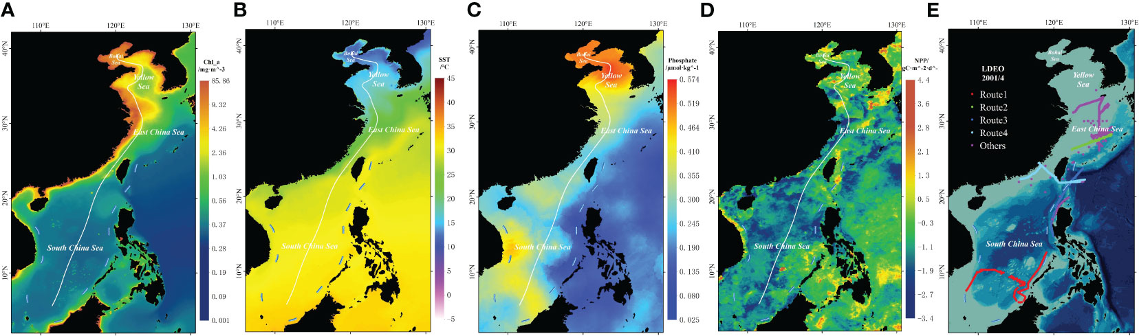
Figure 1 Sampling area of chlorophyll a concentration (A) versus sea surface temperature (B), nutrient salinity (C), net primary productivity of the ocean (D), and pCO₂ data (E). The solid white line in the figure represents the sampling path. Among the nutrients, phosphate is used as a representative for the argument (C), and all three nutrients were actually collected.

2.2.2 Physical and chemical characteristics data of seawater

The sea surface temperature (SST) data is the SST L3 data product from the NASA Oceancolor website, which was also acquired by the MODIS sensor on board the Aqua satellite. And the product used for the study is a composite of the entire mission from July 2002 to August 2020, with a spatial resolution of 4 km. The data product is based on an improved version of the nonlinear SST algorithm (NLSST) of Walton et al. (1998) and uses empirical coefficients derived from regression of in situ and satellite measurements. The sampling points of the SST used for analysis with Chl-a concentration are shown in Figure 1B.

The nutrient (Garcia et al., 2018) and the mixed layer depth (Garcia et al., 2019) data were obtained from the NOAA world ocean atlas website (WOA, https://www.ncei.noaa.gov/access/world-ocean-atlas-2018f/). WOA is the data result after analysis and quality control based on the World Ocean Data Database (WOD) (Takahashi et al., 2020) The nutrient salt data used in this study were respectively the annual data of phosphate, nitrate and silicate in WOA 2009, 2013 and 2018, with a spatial resolution of 1°. These three years were chosen mainly because there were missing data due to different spatial locations in different years of the data, while the data for these three years were completer and more suitable for analytical processing. This study focused on the nutrient salt concentration on the ocean surface. The mixed layer depth data was obtained using January and July 2018 WOA data with a spatial resolution of 0.25°. The sampling points of nutrient salts used for analysis with Chl-a concentration are shown in Figure 1C.

Ocean net primary productivity (NPP) data was obtained from the Marine Science Data Center of the Chinese Academy of Sciences (http://msdc.qdio.ac.cn). The NPP data are the global 9 km ocean primary productivity distance level dataset from 1998 to 2018 (Xue, 2019), and the data used for analysis in this study is December 2018 data with a spatial resolution of 9 km. The data format is GeoTIFF, using the WGS-84 projection coordinate system. The sampling points of NPP used for analysis with Chl-a concentration are shown in Figure 1D.

Surface seawater partial pressure of carbon dioxide (pCO₂) data were obtained from the NOAA Marine Carbon and Acidification Data System (Takahashi et al., 2020) (OCADS, https://www.ncei.noaa.gov/products/ocean-carbon-acidification-data-system) global surface pCO₂ (LDEO) 2019 version of the data set. The dataset is based on direct seawater p_CO2 measurements using the balancer-CO₂ analyzer system from continuous navigation system observations and major national and international oceanographic programs. The spatial and temporal distribution of the LDEO V2019 data is uneven. A large number of measurements are concentrated in the coastal areas of Europe, eastern Japan and North America, while the number of measurements in the waters of China is relatively small. After data screening and comparing the spatio-temporal coincidence degree with other data, the study selected the measured data of LDEO V2019 data set in April 2001. The sampling points of pCO2 used for analysis with Chl-a concentration are shown in Figure 1E.

2.2.3 Marine algae data

Data on marine algae were obtained from the Ocean Biogeographic Information System (OBIS, 2023), and data on the distribution of algae in the eastern coastal region of China were selected. Species selection was based on the top eight species of marine algae observed in greatest numbers.

2.3 Research methodology

2.3.1 Spatial analysis

In terms of spatial change, this study combines monthly data at different time scales to analyze spatial change. Due to the influence of cloud cover and sensor performance, the monthly data is empty for the unscanned data, that is, no data is given. Due to the relatively loose “hollowing” range of empty values, small voids and different positions, a part of error can be offset after operation. Therefore, sampling and interpolation are carried out to eliminate voids, and then raster operation is performed on the image after interpolation, annual Chl-a concentration data were generated.

Based on the synthetic annual data, the cumulative difference method was used to investigate the specific spatial variation. The cumulative difference formula is expressed as:

$\begin{array}{ll}\Delta =\left(2022-2021\right)+\left(2021-2020\right)+\dots +\left(2005-2004\right)+\left(2004-2003\right)& (1)\end{array}$

Numbers indicate year.

At the same time, we used the coefficient of variation to examine spatial heterogeneity. The coefficient of variation (CV) is the ratio of the standard deviation (σ) to mean (μ) (Getis and Ord, 1992). The calculation formula is as follows:

$\begin{array}{ll}CV=\sigma /\mu & (2)\end{array}$

where “σ” and “μ” are calculated from the data of regional spatial distribution data, respectively (Getis and Ord, 1992).

2.3.2 Time analysis

Using satellite remote sensing data analysis software SeaDAS data to extract monthly NC file data. Taking Bohai Sea, Yellow Sea, East China Sea and South China Sea as mask areas, we used SeaDAS statistical function to extract data including mean value, maximum value, minimum value and concentration threshold percentage of Chl-a concentration from the four major sea areas of China and reconstruct the Chl-a concentration time data of the long time series from 2002 to 2022, which provided the data basis for the subsequent time distribution analysis. The coefficient of variation was used to study the fluctuations over time and was calculated as in equation (2), where “σ” and “μ” are calculated using the extracted statistics, respectively.

2.3.3 Trend analysis

The slope function is used to calculate the slope (i.e. trend) of a linear regression model. It is based on the least squares method of fitting a linear equation to find the line of best fit. The slope function is commonly used to analyze long-term trends in time series data. (Montgomery et al., 2012). We used slope analysis to trend the mean Chl-a concentration for long time series. Slope>0 indicates that Chl-a concentration presents an increasing trend over time, while slope<0 indicates that Chl-a concentration presents a decreasing trend. Formula for calculating the slope coefficient (Groebner et al, 2018):

$\begin{array}{ll}slope= \frac{{\displaystyle \sum \left[(x_i-\overline{x})(y_i-\overline{y})\right]}}{{\displaystyle \sum (\overline{x}-x_i)}}& (3)\end{array}$

$x_i$ is for each month from 2002 to 2022; $y_i$ is the average concentration of Chl-a in each ocean region for each month; $\overline{x}$ is the monthly average, $\overline{y}$ is the monthly mean Chl-a concentration in all months from 2002 to 2022.

2.3.4 Time series decomposition

Time series decomposition is a method of breaking down time series data into its component parts, including trends, seasonality, and residuals. This decomposition can help us better understand the characteristics and structure of time series (Hamilton, 1994). Seasonality indicates the recurrence of fluctuations in time series data over a fixed time interval (e.g., annually, quarterly, monthly). Commonly used seasonality models include additive and multiplicative models. In this study, the additive model is chosen. Additive Model: time series = trend + seasonality + residuals.

The equation for time series decomposition can be expressed as

$\begin{array}{ll}\text{Y(t) = T(t) + S(t) + R(t)}& (4)\end{array}$

where Y(t) denotes the time series observations at moment t, T(t) denotes the trend component at moment t, S(t) denotes the seasonal component at moment t, and R(t) denotes the residual component at moment t (Chatfield, 2004).

In this study for the four seas Chl-a concentration time series were decomposed by time series in steps of one month to twelve months, and the step with the most appropriate length was selected for analysis.

2.3.5 Autocorrelation function

The autocorrelation function (ACF) provides insight into the presence of periodicities and repetitive patterns in a time series by calculating the autocorrelation coefficients of the time series at different lagged moments. If the time series is periodic, then its ACF will show the presence of significant peaks or periodic patterns at certain lagged values. These peaks correspond to periodic repetitions in the time series.

The formula for the Autocorrelation Function (ACF) is shown below:

$\begin{array}{ll}\text{ACF}\left(\text{k}\right)\text{=}\left(\text{Cov}\left(\text{X}\left(\text{t}\right)\text{, X}\left(\text{t-k}\right)\right)\right)\text{/}\left(\text{Var}\left(\text{X}\left(\text{t}\right)\right)\right)& (5)\end{array}$

where ACF(k) denotes the autocorrelation coefficient with lag k. Cov(X(t), X(t-k)) denotes the covariance of X(t) with X(t-k). Var(X(t)) denotes the variance of X(t) (Hamilton, 1994).

3 Results and discussion

3.1 Spatial distribution characteristics of Chl-a concentration

Figure 2 and Table 1 show the multi-year average Chl-a concentration, cumulative concentration changes and average temporal coefficients of variation in China Seas from 2002 to 2022.

FIGURE 2

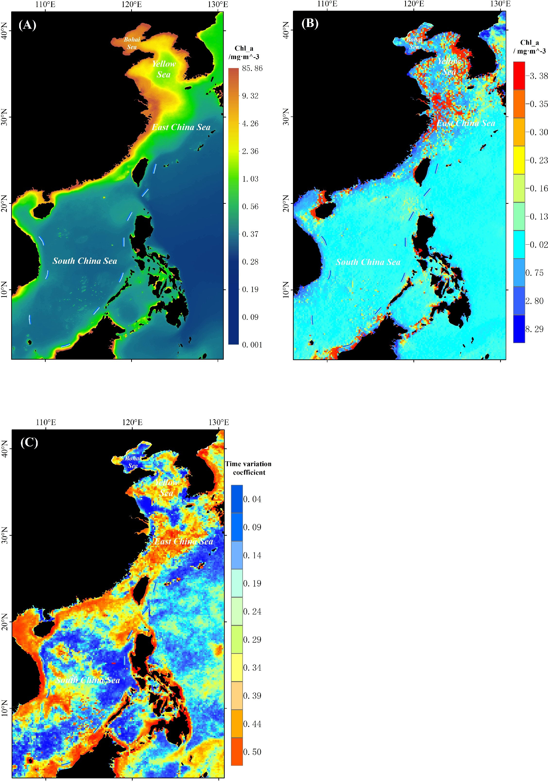
Figure 2 Multi-year average chlorophyll a concentration distribution (A), Cumulative change of multi-year chlorophyll a concentration (B) and time variation coefficient of multi-year chlorophyll a concentration (C) in China seas from 2002 to 2022. Both cumulative concentration changes and temporal coefficients of variation were calculated using equations (1) and (2) for the year-by-year average chlorophyll a concentration values from 2002 to 2022 on the basis of the spatial distribution of the synthesized annual chlorophyll a concentration.

TABLE 1

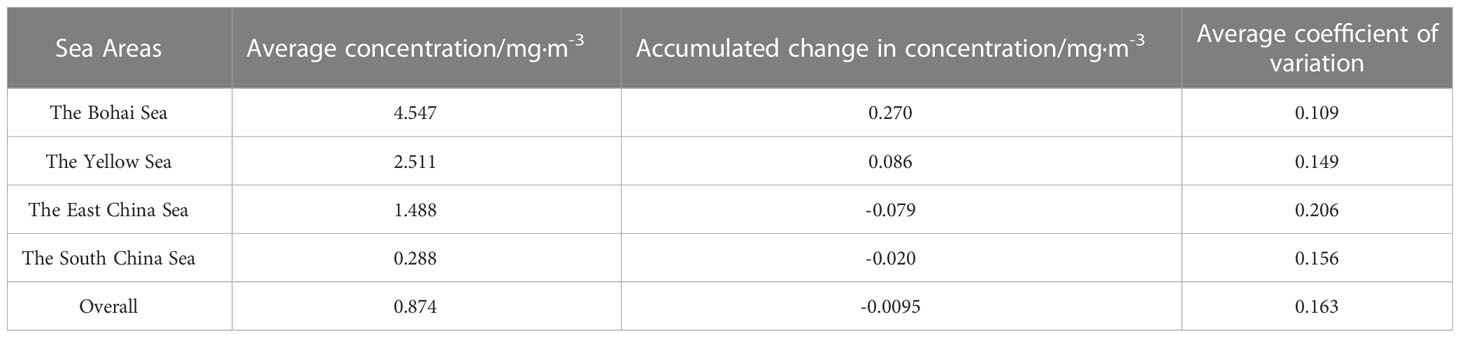
Table 1 Multi-year average chlorophyll a concentration, Cumulative change of chlorophyll a concentration and time variation coefficient of chlorophyll a concentration in China seas from 2002 to 2022.

Figure 2A shows the spatial distribution characteristics of Chl-a concentration in China, the average multi-year Chl-a concentration from 2002 to 2022 is 0.8741 mg/m³, 80% of the sea area Chl-a concentration is below 1.331 mg/m³, 95% of the sea area Chl-a concentration is below 4.159 mg/m³. It can be seen from the Figure 2A that the spatial distribution of Chl-a concentration in China Seas varies significantly over the years, with the Chl-a concentration reaching an extreme value of 48.022 mg/m³ in some nearshore waters and a minimum value of 0.084 mg/m³ in the vast offshore waters, with the high value areas mainly concentrated in the Bohai Sea waters and along the narrow range of the nearshore, while the Chl-a concentration is also high in the Yellow Sea and the eastern part of the East China Sea; The low value area is mainly concentrated in the vast sea area of the South China Sea; as shown in Table 1, the average Chl-a concentration in the Bohai Sea from 2002 to 2022 is 4.547 mg/m³, the average Chl-a concentration in the Yellow Sea is 2.511 mg/m³, the average Chl-a concentration in the East China Sea is 1.488 mg/m³, and the average concentration of Chl-a in the South China Sea is 0.288 mg/m³. The multi-year average Chl-a concentration in each sea area is from high to low in the order of Bohai Sea, Yellow Sea, East China Sea and South China Sea. The average Chl-a concentration in the coastal sea is higher than that in the outer sea, and the Chl-a concentration decreases from the coastal sea to the outer sea, and the Chl-a concentration gradually increases from south to north in each sea.

Figure 2B shows the cumulative difference of Chl-a concentration from 2003 to 2022, and the red areas are the areas with decreasing Chl-a concentration. In addition, the Chl-a concentration in the northern part of the Bohai Sea, the Yellow Sea and the discontinuous coastal waters in the western part of the East China Sea also decreases significantly. Overall, as shown in Table 1, the Chl-a concentration in China Seas showed a decrease from 2002 to 2022. Specifically, the concentration decreased by 0.0095 mg/m³ overall. In the Bohai Sea, the Chl-a concentration decreased by 0.270 mg/m³, while in the Yellow Sea, it decreased by 0.086 mg/m³. Similarly, the East China Sea experienced a decrease of 0.079 mg/m³ in Chl-a concentration, and the South China Sea observed a decrease of 0.020 mg/m³. The overall decrease in Chl-a concentration in China Seas has a negative impact on the marine and global ecological environment. The decrease in Chl-a concentration affects the photosynthesis of marine phytoplankton and algae, leading to a decrease in marine productivity and a negative impact on marine energy flow, which in turn has a negative effect on the marine biological ecological chain. In addition, marine Chl-also profoundly affects the global ecological carbon cycle. Chl-a is the main pigment for photosynthesis of marine phytoplankton, and the decrease in Chl-a concentration reduces the photosynthesis of phytoplankton, which in turn leads to a decrease in the ocean’s carbon sequestration capacity.

In terms of spatial variation, as shown in Figure 2C, the closer the color is to red, the larger the temporal coefficient of variation is, and the greater the fluctuation variation of Chl-a concentration in this space. The average temporal coefficient of variation in the Bohai Sea is 0.1092, which is the least spatially variable among the four major seas in China, and the distribution of Chl-a concentration is the most stable. From the Figure 2C, we can see that the temporal coefficient of variation in the East China Sea is larger, with an average coefficient of variation of 0.2063, and the spatial distribution of Chl-a concentration is the most unstable. Besides, the spatial distribution of Chl-a concentration in the South China Sea is unstable, and the temporal coefficient of variation is also larger in the central-western and northern coasts of the South China Sea and the offshore areas.

3.2 Seasonal variation of Chl-a concentration

Figures 3, 4 show the seasonal variation of the multi-year average Chl-a concentration in China Seas. It is clear from the Figures 3, 4 that the Chl-a concentration in the Yellow Sea and East China Sea reaches its highest values in winter throughout the year, and the concentrations in the Bohai Sea is generally very high throughout the year. The seasonal differences are most pronounced in the vast intersection of the central Yellow Sea waters and the estuary of the Yangtze River. The seasonal differences in Chl-a concentration were most significant in the Bohai Sea and the Yellow Sea, and the seasonal changes in Chl-a concentration were smaller in the East China Sea and the South China Sea.

FIGURE 3

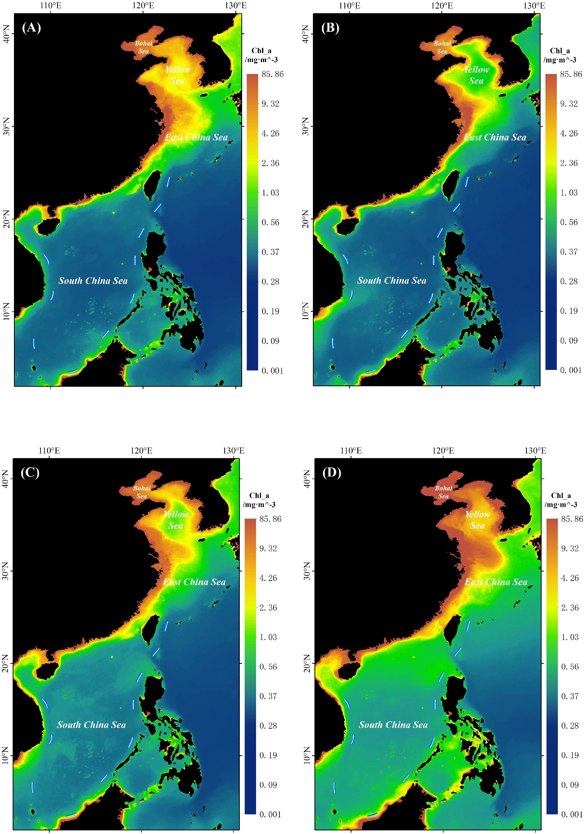
Figure 3 Distribution of multi-year average chlorophyll a concentration by season in China seas from 2002 to 2022. (A)Spring, (B)Summer, (C)Autumn, (D)Winter.

FIGURE 4

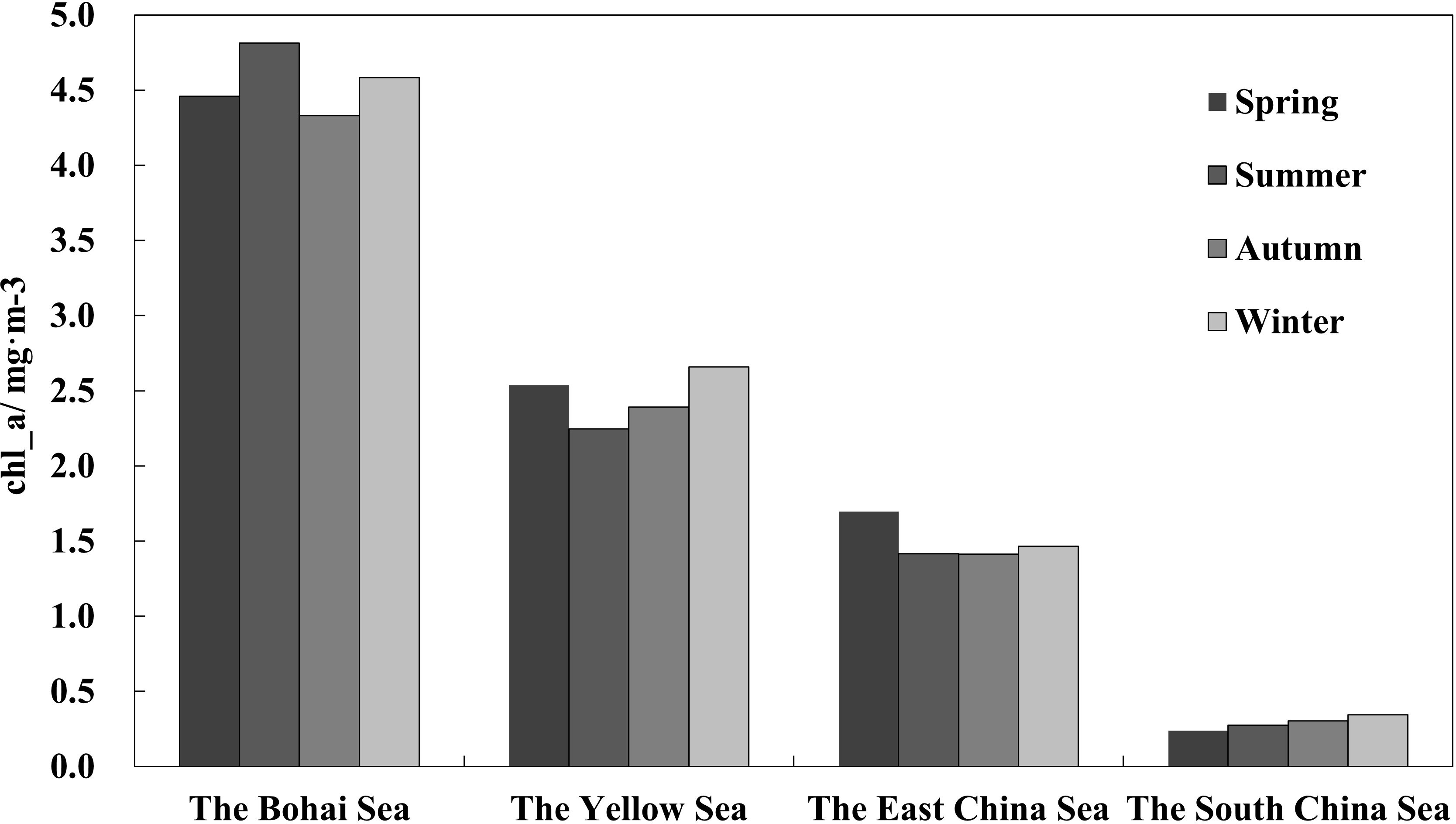
Figure 4 Comparison of the average chlorophyll a concentration in four major seas of China: Bohai Sea, Yellow Sea, East China Sea and South China Sea from 2002 to 2022 and the differences in seasonal chlorophyll a concentration in the four major seas.

As shown in Table 2, the total Chl-a concentration in China Seas reached the maximum value of 0.914 mg/m³ in winter and the lowest Chl-a concentration of 0.832 mg/m³ in summer, with a seasonal distribution of Chl-a concentration throughout the year of winter > spring > autumn > summer. The seasonal distribution of Chl-a concentration varies among the seas. By region, the Chl-a concentration in the Bohai Sea was summer > winter > spring > autumn, in the Yellow Sea was winter > spring > autumn > summer, in the East China Sea was spring > winter > summer > autumn, and in the South China Sea was winter > autumn > summer > spring.

TABLE 2

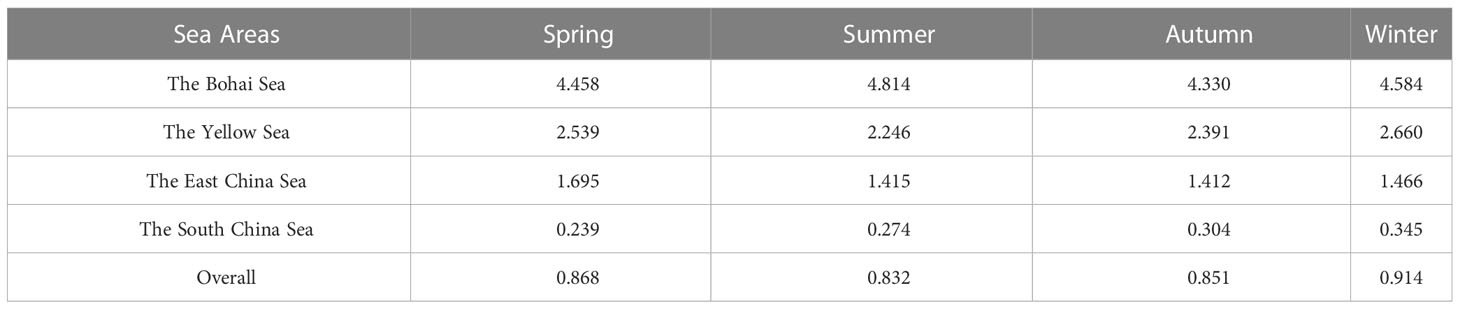
Table 2 Average chlorophyll a concentration(mg/m³) in four major China seas at different periods.

We noticed significant differences in the status of Chl-a concentration in different seasons in different China Seas. This is mainly related to the seasonal dominance of Chl-a in different seas. We have discussed this significant difference in more detail in Section 3.5 below.

3.3 Interannual variation of Chl-a concentration

Figure 5 shows the monthly variation characteristics of Chl-a concentration in four major China Seas from August 2002 to December 2022.It is clear from the Figure that Chl-a concentration shows a clear seasonal cycle, indicating that Chl-a concentration is most influenced by seasonal temperature factors. The graph clearly shows that there are significant differences in Chl-a concentration between the seas, with the highest Chl-a concentration in the Bohai Sea, followed by the Yellow Sea, and the lowest in the South China Sea, showing clear latitudinal differences. The graph shows that the monthly mean Chl-a concentration in the four major China Seas shows a clear periodic variation with the month, while the month corresponding to the high and low variation of Chl-a concentration varies from one sea to another. As shown in Table 3, according to the slope analysis, the slope values of the Bohai Sea and the South China Sea are less than zero and show a trend of decreasing concentration, while the slope values of the Yellow Sea and the East China Sea are greater than zero and show a trend of increasing concentration, and the trend of decreasing Chl-a concentration in the South China Sea is the most obvious. Due to the lack of the latest long-term changes in Chl-a concentration, we compared it with previous studies. Zhao et al. (2019); Zhu et al. (2010); Jun and Liu (2015) investigated the temporal and spatial variations of Chl-a concentration in China Seas at different time scales, and the results showed that Chl-a concentration in Bohai and Yellow Sea waters showed an increasing trend for a long time (Jun and Liu (2015): slope=0.0063 and slope=0.0013 from 1997 to 2012), which are consistent with our research results (Bohai Sea slope=0.0567 and Yellow Sea slope=0.0266 from 2002 to 2013). He et al. (2013) also found that the bloom intensity in the Bohai Sea and the Yellow Sea doubled from 1998 to 2011, which also reflected the high rise of Chl-a concentration in the Bohai Sea and the Yellow Sea during this period, which was confirmed by our study (Chl-a concentration slope=0.0752 in the Bohai Sea from 2002 to 2011, Yellow Sea Chl-a concentration slope=0.0146).

FIGURE 5

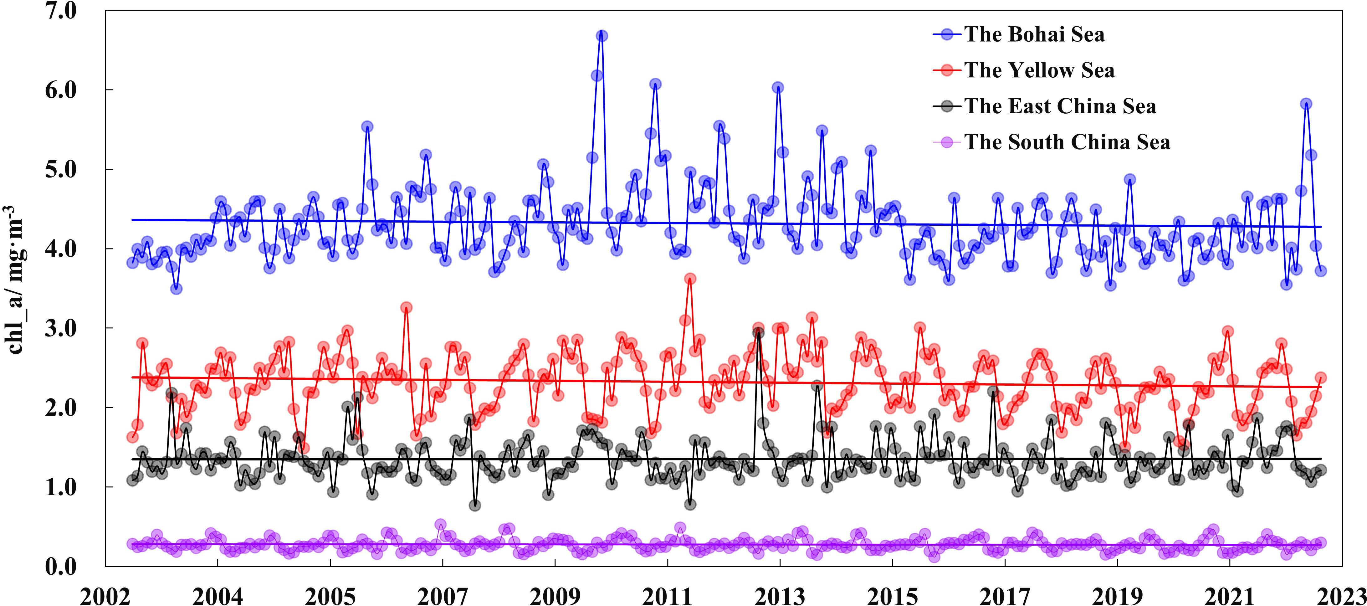
Figure 5 Monthly average chlorophyll a concentration in four major China Seas for a long time series from 2002 to 2022.

TABLE 3

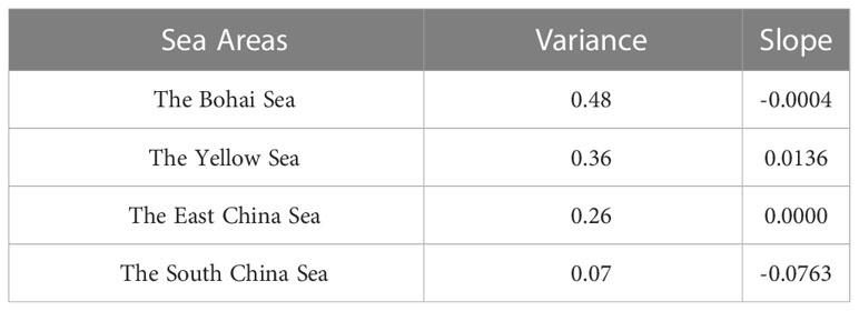
Table 3 Multi-year chlorophyll a concentration variance and slope values in four major China Seas from 2002 to 2022.

In order to investigate whether Chl-a concentration changes are cyclical, an autocorrelation analysis was first performed. Observe the autocorrelation function image Figure 6, the autocorrelation function graph of the Yellow Sea chl_a concentration time series has an obvious trend of periodic changes, the graph shows a symmetrical distribution about the lag order of the horizontal axis, and there are significant peaks at a specific lag order. The autocorrelation coefficients in the autocorrelation function image of Yellow Sea chl_a concentration time series decreases slowly and regularly with the increase of the lag order, not abruptly truncating the tail. The above analysis of the autocorrelation function graphs of the Yellow Sea chl_a concentration time series can be concluded that the Yellow Sea chl_a concentration time series has a more obvious periodicity. It should be pointed out here that the other three seas are not free from the phenomenon of periodicity, but the phenomenon of periodicity of chl_a concentration in the Yellow Sea is more significant. In addition, observing the graph of autocorrelation function, by looking for the peak and decay rate, with the principle that higher peak and slower decay rate indicate stronger periodicity, we can also see that the periodicity of South China Sea chl_a concentration is also more obvious.

FIGURE 6

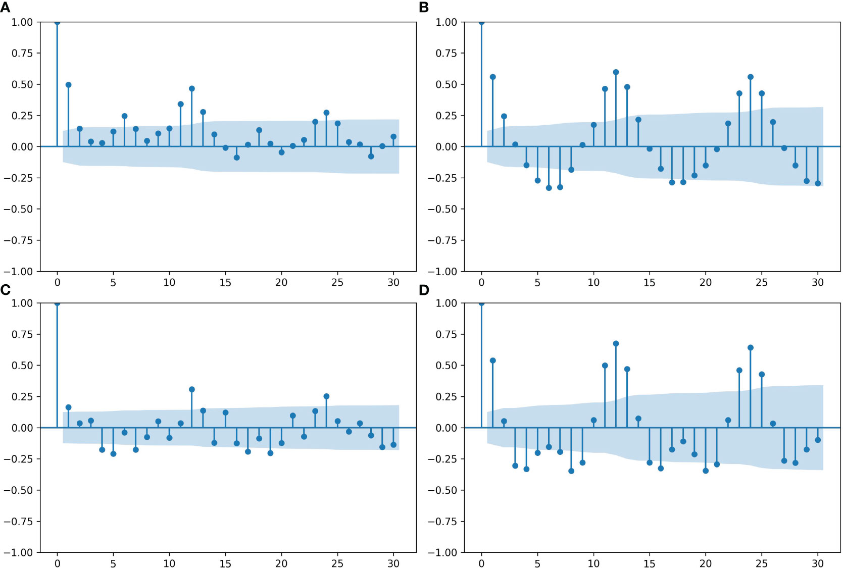
Figure 6 The autocorrelation function images of four sea areas. (A) Bohai Sea, (B) the Yellow Sea, (C) the East China Sea, and (D) the South China Sea. The blue solid points are the autocorrelation function values, and the blue shaded area is the confidence interval.

By decomposing the time series in steps of one month to twelve months, the most appropriate step size is four months. The time decomposition of the original time series is carried out, and the decomposition time length is 4, i.e. the time step is four months. As shown in Figure 7, the numbers 1, 2, 3 and 4 in each column represent the Bohai Sea, Yellow Sea, East Sea and South China Sea respectively, and the graphs in each column from the first column on the left represent the original time series of chl_a concentration, the trend series of chl_a concentration, the seasonal series of chl_a concentration and the residual series of chl_a concentration respectively. The second column of trend series can be regarded as the simulation of the graphical form of the first column of the original time series or the rounded performance of the curve. Comparing the data in the first two columns, it can be seen that the Yellow Sea and the South China Sea have a more obvious cyclical phenomenon compared with the Bohai Sea and the East China Sea, which is due to the differences caused by the closed sea area of the Bohai Sea, the large influence of human activities, and the large exchange of energy of land-based materials in the East China Sea. By observing the seasonal series, we can find out whether there is a fixed cyclical pattern in the data. The seasonal series of the four seas show a repeating pattern of fluctuations, indicating the existence of seasonal influences, the most obvious being temperature. Analysis of the residual series can reveal the part of the original series that is not explained by the trend and seasonality, i.e., the residual term. It can be seen that there is no obvious pattern in the residual series of the four seas, indicating that the trend and seasonality have been well explained in the model. (Note that here the seasonal series in columns three and four as well as the residual series are shown only for the graphical images of 2016-2020 due to the high density of the graph.)

FIGURE 7

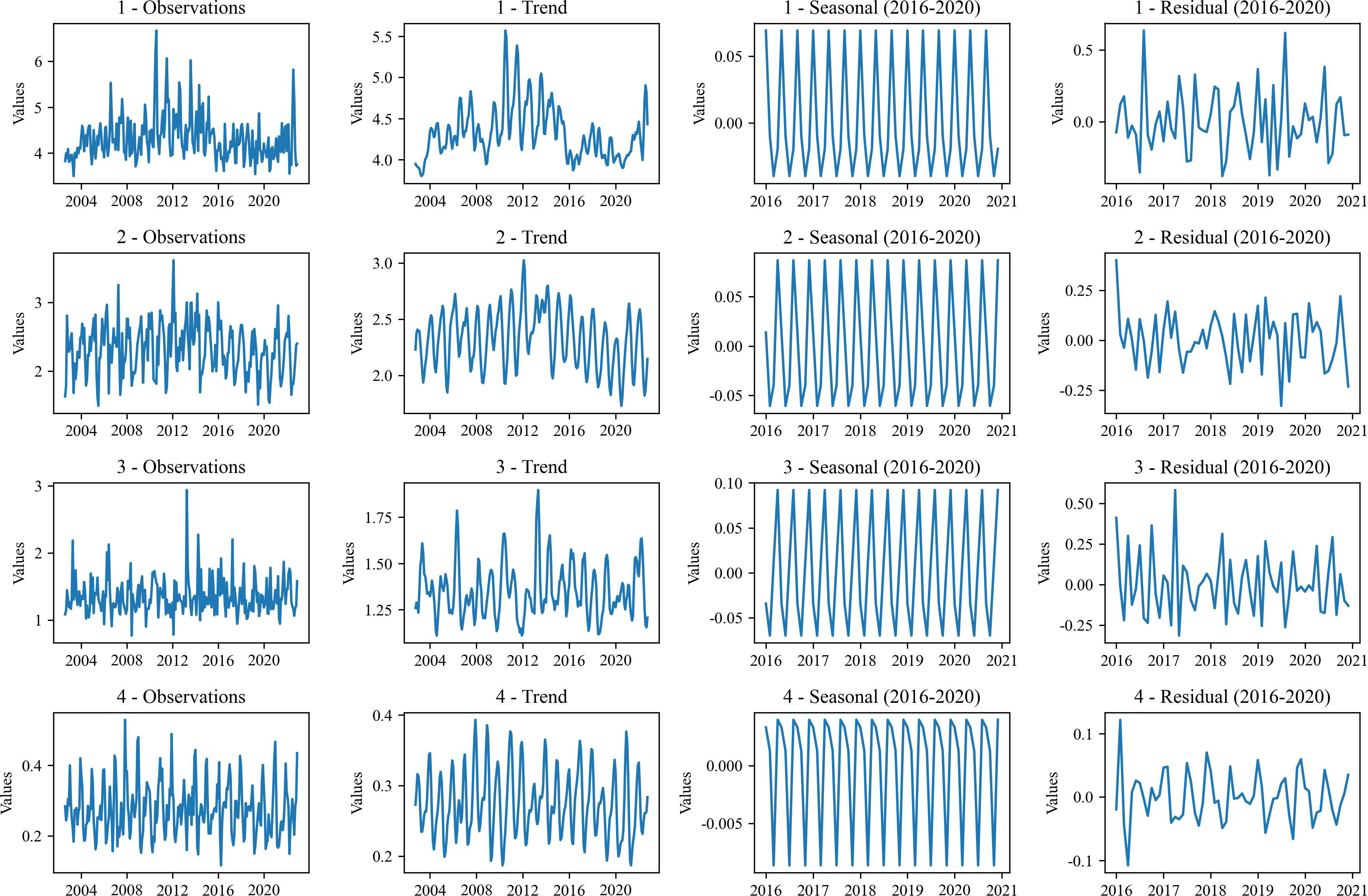
Figure 7 Time decomposition analysis plots of chlorophyll a concentration time series for the four sea areas. Serial number one represents the Bohai Sea, serial number two represents the Yellow Sea, serial number three represents the East China Sea, and serial number four represents the South China Sea. The first column of images represents the original time series plot, the second column represents the trend plot after time decomposition, the third column represents the seasonal component plot after time decomposition, and the fourth column represents the residual plot after time decomposition.

Figure 8 and Table 3 show the average Chl-a concentration values, the temporal coefficient of variation and the variance for each year in each sea area. The variance of the monthly Chl-a concentration in the Bohai Sea during this period was 0.48, while the interannual variation of the temporal coefficient of variation was large, indicating that the interannual variation of the Chl-a concentration in the Bohai Sea was highly variable and the temporal distribution of the Chl-a concentration was unstable. There are obvious anomalies in the variation of the long time series, as shown in Figures 5 , 6. Within 2010 to 2013, the monthly mean Chl-a concentration fluctuated the most, and the coefficient of temporal variation was generally large. The data collection revealed that sudden and rare ice conditions occurred in Liaodong Bay, Bohai Bay, Laizhou Bay and the northern Yellow Sea and Jiaozhou Bay in the Bohai Sea in 2010 (Sun et al., 2011), and the CNOOC oil spill in Bohai Bay in 2011 (Chen, 2013), indicating that the influence of environmental or human factors may cause fluctuating changes in Chl-a concentration. The interannual variation of the coefficient of temporal variation in the South China Sea is not too high and the variance of Chl-a concentration in each month during this period is 0.07. The interannual distribution of Chl-a concentration is stable, which is largely related to the latitude distribution, sea area and sea distribution. The high latitude of the Bohai Sea results in greater temperature fluctuations. And the sea area is smaller and more occluded, and the human population density is higher. The change of human discharge of various types of production and living materials into the Bohai Sea leads to a greater interannual variation of Chl-a concentration in the Bohai Sea. In addition, there are significant interannual differences in the flow of rivers entering the Bohai Sea. The decrease in inlet water flow during dry periods and the increase in inlet river flow during rainy periods in turn have an impact on the interannual variation of Chl-a concentration. The South China Sea, on the other hand, is an open and large area, which has a stronger regulating effect on Chl-a. Moreover, the South China Sea is located at low latitudes, where seasonal fluctuations in temperature are small, which in turn causes small seasonal variations in Chl-a concentration. In addition, based on the temporal coefficient of variation, it can be concluded that the interannual fluctuations of Chl-a concentration in the Bohai Sea and the East China Sea show an increasing trend, while the interannual fluctuations of Chl-a concentration in the Yellow Sea and the South China Sea do not vary significantly.

FIGURE 8

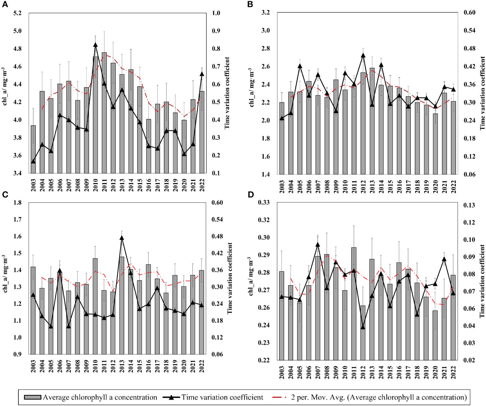
Figure 8 Multi-year annual average chlorophyll a concentration and time variation coefficient of the four major China seas from 2002 to 2022. (A) Bohai Sea, (B)Yellow Sea, (C)East China Sea, (D)South China Sea. The coefficient of temporal variation for each year was calculated from the monthly chlorophyll a concentration values for that year. The red dotted line in the figures is a moving average simulation of the annual change in chlorophyll a concentration for each sea area.

3.4 Correlation analysis of Chl-a concentration and physicochemical characteristics of seawater

3.4.1 Chl-a and seawater physical and chemical characteristics

Since some data are missing at some locations on the sampling line, the ARIMA model (Box et al, 2015) was firstly used to fit at the maximum extent, on the basis of which the analysis was carried out in the observation.

As shown in Figure 9A, analysis of the relationship between temperature and Chl-a concentration shows a non-linear relationship, with Chl-a concentration showing some fluctuation or threshold effect with the change of seawater temperature. The positive correlation on a certain interval is due to the fact that higher temperature can provide a more favorable growth environment and promote the growth and reproduction of phytoplankton, which leads to an increase in Chl-a concentration. And a negative correlation on a certain interval, this is because high temperature may lead to the acceleration of metabolic processes in phytoplankton, which increases their demand for nutrients and also accelerates the consumption of photosynthesis products, thus decreasing Chl-a concentration.

FIGURE 9

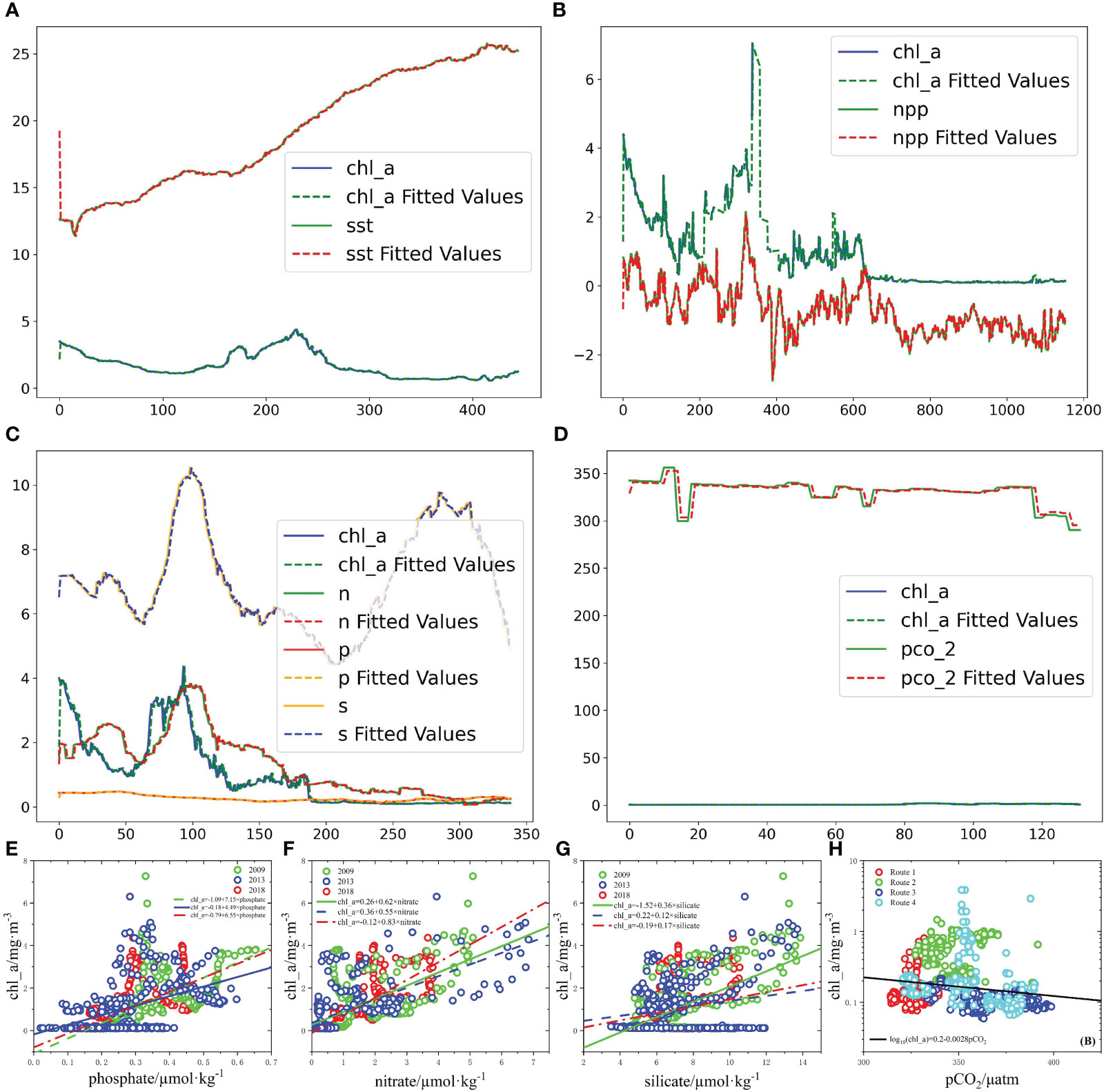
Figure 9 (A) Correlation between chlorophyll a concentration and seawater surface temperature as shown, (B) correlation between chlorophyll a concentration and net primary productivity of the ocean, (C) correlation between chlorophyll a concentration and nitrate, phosphate, and silicate, and (D) correlation between chlorophyll a concentration and partial pressure of carbon dioxide in seawater. The dotted lines in the above plots are the curves after each data has been fitted by ARIMA time model. Note that for simplicity of study, (A–D) are dimensionless. (E–G) are the regression plots of phosphate, nitrate, and silicate with chlorophyll a concentration, respectively, and (H) is the regression plot of seawater carbon dioxide partial pressure with chlorophyll a concentration on the four sampling lines.

Because Chl-a concentration directly affects the intensity of biological photosynthesis, it is also an important characteristic quantity to characterize biological productivity. On the one hand, the increase of Chl-a concentration promotes the photosynthesis of marine phytoplankton, and under the condition of certain energy consumption by itself, the accumulated organic matter increases and the net primary productivity increases; on the other hand, when the net primary productivity of marine phytoplankton is increased by other factors, the phytoplankton On the other hand, when the net primary productivity of marine phytoplankton increases due to other factors, the photosynthetic efficiency will also increase, promoting itself to produce more Chl-a to meet the photosynthetic load. So there is an overall synergistic change between the two in the Figure 9B.

Observing the Figure 9C, it can be roughly seen that the three nutrients and Chl-a concentration also show a trend of synergistic change, but not very obvious. So phosphate, nitrate, and silicate were extracted from the ocean surface on the sampling route in 2009, 2013, and 2018, respectively, and regressed with Chl-a. The results are shown in Figures 9E–G, respectively. All three nutrient salts have different degrees of contribution to Chl-a. Phosphate had the most significant promotion effect on Chl-a concentration, followed by nitrate, and silicate had the weakest promotion effect on Chl-a concentration. The concentration of phosphate in seawater is the lowest among the three nutrients, but small changes in its concentration have the greatest effect on Chl-a. Poornima et al. (2014) analyzed the relationship between Chl-and phosphate in an experiment using in situ nutrient enrichment experiments and showed significant uptake and utilization of phosphate by phytoplankton. Numerous studies on HABs have also shown that phosphorus deficiency greatly inhibits the growth of HABs (Adolf et al., 2009; Au et al., 2010; Guan and Ping, 2017; Lema et al., 2017), which in turn can affect Chl-a concentrations. In addition, the annual average concentrations of phosphate, nitrate, and silicate in China Seas in 2009, 2013, and 2018 (Table 4) showed a decreasing trend in all three nutrient concentrations in China Seas to varying degrees. 2018 phosphate concentrations decreased by 11.51%, nitrate by 2.87%, and silicate by 2.46% compared to 2009, which also corroborates the overall decrease of Chl-a concentration in China Seas by -0.0095 mg/m³ over 20 years.

TABLE 4

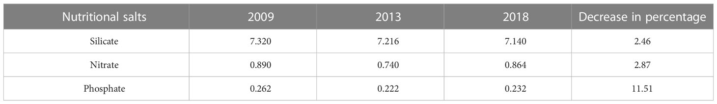
Table 4 Annual average values of three nutrients (μmol/kg) and percentage decrease in 2009, 2013 and 2018.

Phytoplankton in the ocean (e.g., algae and phytoplankton) absorb light energy through photosynthesis and use carbon dioxide and water to synthesize organic matter, while releasing oxygen. This process regulates pCO₂ in seawater, so Chl-a concentration is strongly related to the partial pressure of carbon dioxide in seawater. As the Figure 9D shows, the relationship between pCO₂ and Chl-a concentration is not obvious. Therefore, the regression analysis was performed on the pCO₂ data collected from cruise lines 1, 2, 3, and 4 and the Chl-a concentration data at the same point in that month, respectively, and the analysis results are shown in Figure 9H. Here again, the logarithm operation was performed on Chl-a. Since the relationship between the two is complex, the direct regression analysis does not portray the relationship well, so after the logarithm processing of Chl-a The two showed a more regular correlation. Bai et al. (2015) proposed a “MeSAA” algorithm to evaluate pCO₂ using temperature, salinity, and Chl-a concentration, and their process analysis also showed a negative correlation. The expression for photosynthesis is as follows (Yuan et al., 2013):

$\begin{array}{ll}{\text{136CO}}_{\text{2}}{\text{+16NO}}_{\text{3}}{}^{\text{-}}{\text{+HPO}}_{\text{4}}{}^{\text{2-}}\text{+0}{\text{.5SO}}_{\text{4}}{}^{\text{2-}}{\text{+85H}}_{\text{2}}{\text{O+19H}}^{+}{\text{=C}}_{\text{136}}{\text{H}}_{\text{190}}{\text{O}}_{\text{37}}{\text{N}}_{\text{16}}{\text{P}}_{\text{1}}{\text{S}}_{\text{0}\text{.5}}{\text{+188O}}_{\text{2}}& (6)\end{array}$

Marine phytoplankton convert dissolved inorganic carbon dissolved in the ocean into organic carbon form through photosynthesis, which directly affects the partial pressure of carbon dioxide in seawater and reduces pCO₂.

3.4.2 Chl-a and seawater dynamics processes

Figures 10A, B show the mixed layer depths in January as well as July 2018.It is clear from the figure that the mixed layer depth in January is generally greater than that in July in China Seas. The seasonal variation of Chl-a concentration in the South China Sea and the East China Sea, for example, the Chl-a concentration in the South China Sea reaches its peak in winter, while the East China Sea reaches its peak in spring, as shown in Figure 10A. Compared with the East China Sea, the northeast monsoon prevails in the South China Sea in winter, and the strong winter wind acts on the sea-air interface, causing the ocean dynamics process, the vertical movement of seawater is significant, and the mixed layer of the water body deepens during the vertical flow of seawater, and the rich nutrients are brought to the surface layer of the ocean under the action of the surge current (Boyd and Trull, 2007), which provides rich material supply for marine phytoplankton, so the Chl-a concentration in the South China Sea is high in winter. Figures 10C, D show the cumulative differences in phosphate concentrations at three different ocean depths in the South China Sea: the ocean surface, 25 m below the sea surface, and 50 m below the sea surface in winter and summer (corresponding to January and July at mixed layer depths, respectively) (phosphate was selected for analysis because it has the greatest effect on Chl-a concentration as analyzed above), and Table 5 shows the phosphate concentrations at different ocean depths in 2018. From the cumulative difference in phosphate concentration across ocean depths, the difference in nutrient concentration with ocean depth in the photosynthetic zone (surface layer of the ocean) becomes smaller compared to summer due to the influence of mixed layer deepening in winter, which allows phosphate in seawater to be transported from deeper ocean areas to shallower layers of seawater, facilitating nutrient supply to phytoplankton in the photosynthetic zone and thus promoting more Chl-a production, which explains the specific influence mechanism of how mixed layer deepening promotes higher Chl-a concentration.

FIGURE 10

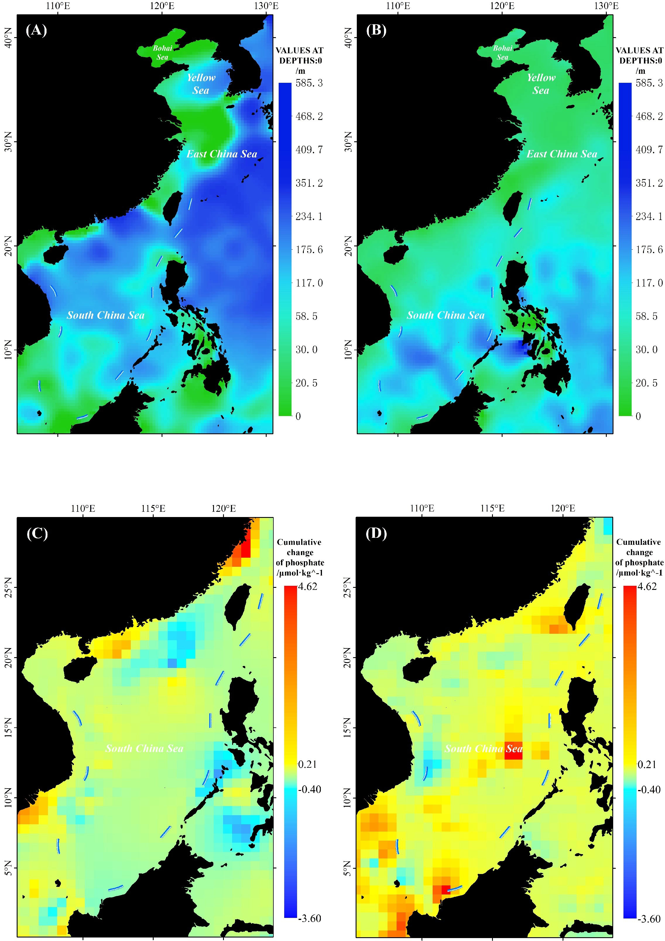
Figure 10 Depth of mixed layer in winter (A) and summer (B) in China Seas in 2018 and cumulative difference between winter (C) and summer (D) concentrations of phosphate at sea level, 25m below sea level, and 50m below sea level in the South China Sea in 2018.

TABLE 5

Table 5 Concentration of phosphate at different sea depths in 2018.

3.5 A comprehensive explanation of the spatial and temporal variation of Chl-a concentration in China Seas by multiple influencing factors of Chl-a

In the context of global warming, the China Seas produces El Niño-like ocean surface temperature anomalies (Dai et al., 2011), and the overall seawater temperature shows an increasing trend, and with the above analysis of the negative correlation between Chl-a and SST, the increase of seawater temperature makes the decrease of Chl-a concentration; in addition, the nutrient salts in the China Seas have decreased to different degrees during 2009-2018, and different nutrient salts play a role in the Therefore, the decrease of nutrient salt concentration is not conducive to the growth of marine phytoplankton, resulting in the decrease of Chl-a concentration. The above analysis explains the overall decrease of 0.0095 mg/m³ in Chl-a concentration in China Seas from 2002 to 2022.

From north to south, the sea surface temperature of the Bohai Sea, Yellow Sea, East Sea and South China Sea shows a decreasing trend, and the negative correlation effect of the temperature factor makes the Chl-a concentration show a decreasing trend; human production activities discharge a large amount of wastewater waste into the ocean, and a large proportion of these substances will cause eutrophication of near-shore seawater, which makes a phenomenon similar to algal bloom, and Chl-a concentration rises, while the near-shore of the Bohai Sea, Yellow Sea, East Sea and South China Sea The population density and number gradually decline, the impact of human activities is different, and the impact on Chl-a concentration is different; in addition, the Bohai Sea is closed, seawater mobility is poor, nutrients are more easily enriched, so the Chl-a concentration is large, while the South China Sea is open, seawater flow phase is strong, seawater exchange capacity is strong, nutrient dispersion mobility is strong, also will have an impact on Chl-a concentration. The above analysis explains the reason why the Chl-a concentration gradually decreases from north to south in four different seas in China.

In section 3.2, we can clearly observe a very clear seasonal difference in Chl-a concentration in different sea areas. The concentration of Chl-a in the Bohai Sea reaches its highest in summer, when the main controlling factor is no longer temperature, but the material and energy output from the land system to the marine system. In summer, the rainfall in northern China and the Loess Plateau area increases significantly, especially the Loess Plateau area has more heavy rainfall, and because of the loose loess soil, a large amount of sediment is carried by rainwater under the erosion of heavy rain pouring through the land runoff process and finally from the Yellow River inlet into the sea, a large amount of sediment in the sea contains a large amount of nutrients, providing rich growth energy for the growth of phytoplankton in the Bohai Sea, so the high concentration of Chl-a in the Bohai Sea in summer Therefore, the concentration of Chl-a in the Bohai Sea is high in summer. The Chl-a concentration in the Yellow Sea is winter>spring>autumn>summer, and its Chl-a concentration is consistent with the seasonal change of temperature and is most regulated by the temperature factor. The Chl-a concentration in the East China Sea reaches its maximum in spring, when the temperature of the East China Sea rises in spring and reaches the temperature required for phytoplankton growth, temperature is no longer a limiting factor, but plays a role in promoting the growth and development of marine phytoplankton, when phytoplankton multiply and marine productivity is improved. The Chl-a concentration in the South China Sea is winter > autumn > summer > spring, and the main influencing factor is the temporal change of nutrient salts regulated by the physical process of seawater (as in section 3.4.2: surge flow, mixed layer changes).

Attempts to establish quantitative relationships between Chl-a and its various influencing factors are very difficult. Not only various influencing factors have an effect on Chl-a, but also various influencing factors interact, influence and change synergistically with each other. As shown in equation (6), marine phytoplankton not only convert dissolved inorganic carbon to organic carbon in the process of photosynthesis, which directly affects seawater pCO₂, but the process is also accompanied by changes in the utilization of various nutrient salts in the reservoir and changes in seawater pH, which further affect pCO₂. Furthermore, changes in nutrient salts in seawater can cause changes in seawater pH, which not only directly affects phytoplankton, but also changes in pH have an effect on the ionization of chemicals in seawater, which further affects the growth and development of phytoplankton. In addition, in different seas and at different times, as analyzed above, the main controlling factors of Chl-a are different, and a generalized summary of the law cannot well describe the complex situation of floating changes of multiple influencing factors.

3.6 Marine fisheries under the influence of spatial and temporal variation of Chl-a concentration in China Seas - Zhoushan fishing grounds as an example

Since the concentration of marine Chl-a can be used as one of the indicators of the abundance of marine phytoplankton and algal organisms, the changes in the concentration of marine chl_a in China essentially reflect the changes in marine plants. Therefore, the following study is conducted from the perspective of marine algal plants to analyze the effects on marine fish.

We analyzed the plant distributions of Thalassia hemprichii, Halophila ovalis, Cymodocea rotundata, Enhalus acoroides, Halodule pinifolia, Zostera subg. Zostera marina, Favites pentagona, Halodule uninervis recorded in the eastern coast of China since 2008-2018 based on OBIS. Zostera subg. Zostera marina, Favites pentagona, Halodule uninervis, and other marine algae were statistically analyzed at the depth of the observed plant distribution according to sea level each year. These eight species of marine plants are found in shallow offshore waters and are usually attached to rocks or other substrates, allowing some fish to use the zooplankton or benthos attached to the algae as an additional food source (Shoji et al., 2010). Some specific fishes, such as Perciformes and Stonefish, are classified as algal-feeding fishes, which feed mainly on algae. These fishes have adapted their digestive systems and oral structures to efficiently digest and ingest algae as their main food source (Payne et al., 2008). Therefore, the growth and distribution of these algae can greatly affect the survival of marine fishes that feed on or depend on algae for their environment.

In our study, as shown in Figure 11, we found that two groups of algae, Thalassia hemprichii and Halophila ovalis, showed an increasing trend of growing sea depth over the years, while the remaining six species, Cymodocea rotundata, Enhalus acoroides, Halodule pinifolia, Zostera subg. Zostera marina, Favites pentagona, and Halodule uninervis plants showed a deepening trend in growing sea depth. We speculate that this is related to global warming. On the one hand, global warming makes the temperature of shallow seawater rise, and since the optimal growth temperature of algal plants is specific, the rise in seawater temperature makes marine plants tend to go to a deeper layer of seawater to meet their optimal habitat. On the other hand, the increase in seawater temperature will have an impact on the dissolved oxygen content in seawater. In general, when seawater temperature increases, the dissolved oxygen content in seawater decreases. (Breitburg et al., 2018) As seawater deepens, dissolved oxygen levels are usually higher due to increased water pressure, so algal plants seek a more suitable supply of oxygen and carbon dioxide in deeper water to promote their own growth.

FIGURE 11

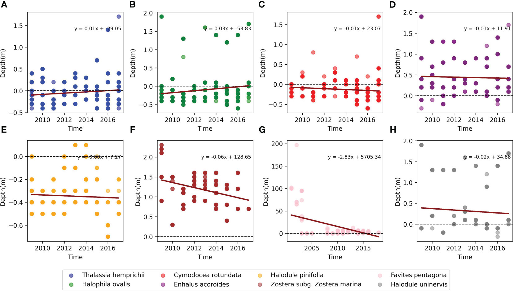
Figure 11 Each graph represents the observed growing water depth of eight marine plants during 2008-2020, with negative values below the sea surface and positive values above the sea surface. (A–H) represent, in order, Thalassia hemprichii, Halophila ovalis, Cymodocea rotundata, Enhalus acoroides, Halodule pinifolia, Zostera subg. Zostera marina. Solid dots represent bathymetric values, black dashed lines represent sea level, and red realizations represent trend changes over years.

The above changing status of marine algal plant habitats corresponds to Figure 2B. Figure 2B concentrates on the long-term evolution of Chl-a concentration in Chinese waters. The tendency of marine algal plant habitats to deeper seawater corresponds to the decrease in cumulative Chl-a concentration in eastern Chinese waters, which corroborate each other. Therefore, the long-term evolution of Chl-a concentration in Chinese waters is a response to the long-term evolution of marine algae. Correspondingly, the impact of Chl-a concentration changes in Chinese waters is essentially the impact of the evolution of marine algae on Chinese waters. Algal plants are the basis of the marine food chain. They produce organic matter through photosynthesis, which serves as bait and a source of nutrients for other organisms. If algal plants grow deeper, this may result in more algal plants growing in deeper waters, which in turn changes the structure and abundance of the food chain. This may have implications for food availability for marine fishes in different strata. (Smale et al., 2019) Because marine ecosystems are an interconnected whole, small changes in the environment in which marine plants grow can also have a large impact on marine fishes.

Located in the northeastern part of Zhejiang Province, east of Hangzhou Bay and southeast of the estuary of the Yangtze River, Zhoushan Fishery is the largest fishery in China, with the four major economic fishes, big yellowtail, small yellowtail, striped bass and squid, as the main aquatic products. The fishery resources have suffered serious damage due to the long-term indiscriminate fishing and marine pollution (Zhu and Qian, 2022).

Marine Chl-a is mainly derived from marine algae, which form the energy base of the aquatic food chain and play a vital role in the aquatic ecosystem. Chl-a concentration is an important basis for judging the growth and production level of marine algae, so the level of Chl-a concentration indirectly reflects the food abundance and habitat quality of fish.

The main purpose of the fishing moratorium is to avoid the peak period of fish growth and reproduction and to prevent the decline of biological populations due to overfishing. As shown in Figure 12, the Chl-a concentration in Zhoushan fishing grounds during the fishing moratorium showed a fluctuating downward trend, reflecting that the growth environment and nutrient synthesis of phytoplankton in the fishing grounds were in a decreasing trend. The food abundance of marine fish had decreased, which was not conducive to the growth and reproduction of marine fish during the golden recovery period of the fishing moratorium, nor was it conducive to the recovery of marine fish resources and the sustainable development of marine fisheries, which were potential challenges for modern fisheries. In order to maintain the sustainable development of marine fisheries, both a reasonable rest-fishing balance and attention to environmental protection are needed to maintain a good growing environment for marine fish and the food sources on which they depend. Meanwhile, according to statistics, the marine fish catch in Zhoushan fishing grounds increased from 1,155,480,000 tons to 1,541,289,000 tons between 2002 and 2021, an increase of 33.4% in 20 years (Zhoushan Bureau of Statistics, 2022). The decline in fish habitat quality caused by the decrease in Chl-a concentration is contrasted with the increasing fishing capacity of Zhoushan fishing ground over the years. The unreasonable fishing activities of contrasted with aggravate the deterioration of the marine ecological environment and lead to the decrease of Chl-a concentration in the fishing ground. Simultaneously, in the face of the decreasing trend of Chl-a concentration, if the human continues to maintain high growth of fishing volume will certainly lead to the depletion of fish resources.

FIGURE 12

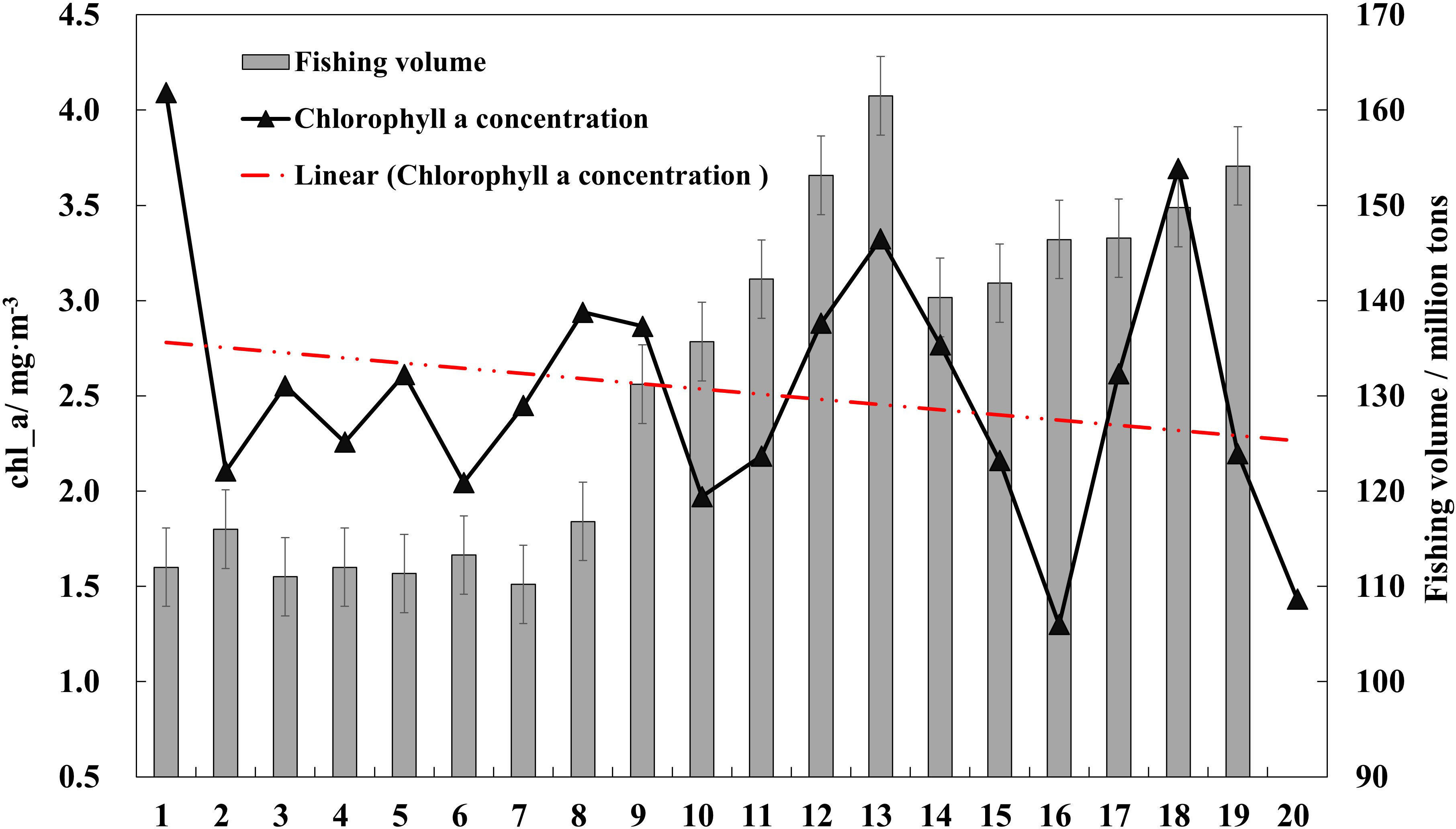
Figure 12 Changes in chlorophyll a concentration during the fishing moratorium in Zhoushan fishery from 2003 to 2022 and changes in fish catch from 2003 to 2021. The red dotted line in the figure is a linear simulation of the annual variation of chlorophyll a concentration during the fishing moratorium in Zhoushan fishery.

4 Concluding remarks

In this study, spatial distribution characteristics data of long time series were constructed to delineate the spatial and temporal variation characteristics of Chl-a concentration in China Seas. In addition, the potential effects of several oceanographic variables on Chl-a concentrations were analyzed. Finally, the potential impacts on marine fisheries and the urgency of sustainable development of marine fisheries were investigated from the essence of changes in Chl-a concentrations and changes in marine algal plants The results of the study showed that:

(1) The multi-year average Chl-a concentration in China Seas from 2002 to 2022 was 0.874 mg/m³. the average Chl-a concentration in Bohai Sea waters over the years was the highest, at 4.547 mg/m³, and in South China Sea waters was the lowest, at 0.288 mg/m³. in terms of spatial variation, the overall Chl-a concentration in China Seas from 2002 to 2022 decreased cumulatively by 0.0095 mg/m³, with the largest cumulative increase of 0.270 mg/m³ in the Bohai Sea and the largest cumulative decrease of 0.079 mg/m³ in the East China Sea. the largest multi-year spatial variation of 0.2063 in the East China Sea indicates that the spatial distribution pattern of Chl-a concentrations has evolved significantly.

(2) In terms of temporal variation, Chl-a concentration in the Bohai Sea in China from 2002 to 2022 showed a decreasing trend, the Yellow Sea showed an increasing trend, the East China Sea remained basically unchanged, and the South China Sea showed a decreasing trend In terms of temporal variation, Chl-a concentration in the Bohai Sea fluctuated significantly from year to year, and there were obvious differences in Chl-a concentration in each year.

(3) The time series of Chl-a concentration changes in the four seas were analyzed by autocorrelation as well as time decomposition analysis, and the changes of Chl-a concentration over a long period of time had obvious periodic phenomena, among which the time decomposition periodicity was most obvious in four-month steps, which was obviously related to seasonal temperature changes. Among them, the cyclical phenomenon was most obvious in the Yellow Sea.

(4) There was an overall negative correlation between Chl-a and sea surface temperature, but the correlation varied between different temperature bands. All three nutrient salts studied promoted Chl-a, with phosphate having the most pronounced promotion effect on Chl-a. Chl-a was negatively correlated with pCO₂. Seasonal changes in the mixed layer had a strong influence on the variation of nutrients in the upper ocean.

(5) There is a trend of increasing water depth for the growth of the studied algae plants, and this change can greatly affect the survival of marine fish that feed on or depend on algae for their environment. The Chl-a concentration in Zhoushan fishing grounds during the fishing moratorium showed a decreasing trend, while the catch of Zhoushan fishing grounds showed an increasing trend year by year. The decrease of Chl-a concentration limits the food source of fish during the fishing moratorium, which is not conducive to the sustainable development of marine fisheries.

Data availability statement

The datasets presented in this study can be found in online repositories. The names of the repository/repositories and accession number(s) can be found below: https://www.ncei.noaa.gov/access/ocean-carbon-acidification-data-system/oceans/LDEO_Underway_Database/ and https://oceancolor.gsfc.nasa.gov/.

Author contributions

XZ contributed to the synthesis of chlorophyll a data. DM and JX contributed to the data visualization. DZ examined and verifiedthe results of the research process data. KZ and YC analyzed the data and drafted the manuscript. All authors participated in the discussion of the data, interpretations, and manuscript revision.

Funding

This work was funded by the National Science Foundation of Fujian Province, China (Grant No. 2022J01818), National Fund Cultivation Program Project of Jimei University (Grant No. ZP2022016), the Fund of Fujian Ocean Synergy Alliance (FOCAL) (Grant No. FOCAL2023-0101), and Independent Research Projects of the Southern Marine Science and Engineering Guangdong Laboratory (Zhuhai) (Grant No. SML2021SP306).

Acknowledgments

The authors express our sincere gratitude to Prof. DQ for his helpful supports as well as the data service provided by the Oceanographic Data Center (Chinese Academy of Sciences, CASODC), National Centers for Environmental Information (NOAA) and NASA EarthData OceanColor Web.

Conflict of interest

The authors declare that the research was conducted in the absence of any commercial or financial relationships that could be construed as a potential conflict of interest.

Publisher’s note

All claims expressed in this article are solely those of the authors and do not necessarily represent those of their affiliated organizations, or those of the publisher, the editors and the reviewers. Any product that may be evaluated in this article, or claim that may be made by its manufacturer, is not guaranteed or endorsed by the publisher.

References

Adolf J. E., Bachvaroff T. R., Place A. R. (2009). Environmental modulation of karlotoxin levels in strains of the cosmopolitan dinoflagellate Karlodinium veneficum (Dinophyceae). J. Phycol. 45, 176–192. doi: 10.1111/j.1529-8817.2008.00641.x

PubMed Abstract | CrossRef Full Text | Google Scholar

Au F. X., Place A. R., Garcia N. S., et al. (2010). CO₂ and phosphate availability control the toxicity of the harmful bloom dinoflagellate Karlodinium veneficum. Aquat. Microbial Ecol. 59, 55–65. doi: 10.3354/ame01396

CrossRef Full Text | Google Scholar

Bai Y., Cai W. J., He X., Zhai W. D., Pan D. L., Dai M. H., et al. (2015). A mechanistic semi-analytical method for remotely sensing sea surface pCO2 in river-dominated coastal oceans: A case study from the East China Sea. J. Geophys. Res. Oceans. 120, 2331–2349. doi: 10.1002/2014JC010632

CrossRef Full Text | Google Scholar

Behrenfeld M. J., Boss E., Siegel D. A., et al. (2005). Carbon-based ocean productivity and phytoplankton physiology from space. Global Biogeochem. Cycles. 19 (1). doi: 10.1029/2004GB002299

CrossRef Full Text | Google Scholar

Blondeau-Patissier D., Gower J. F., Dekker A. G., et al. (2014). A review of ocean color remote sensing methods and statistical techniques for the detection, mapping and analysis of phytoplankton blooms in coastal and open oceans. Prog. Oceanography. 123, 123–144. doi: 10.1016/j.pocean.2013.12.008

CrossRef Full Text | Google Scholar

Box G. E., Jenkins G. M., Reinsel G. C., Ljung G. M. (2015). Time series analysis: forecasting and control. Hoboken, NY: John Wiley Sons.

Google Scholar

Boyd P. W., Trull T. W. (2007). Understanding the export of biogenic particles in oceanic waters: Is there consensus? Prog. Oceanography 72 (4), 276–312. doi: 10.1016/j.pocean.2006.10.007

CrossRef Full Text | Google Scholar

Breitburg D., Levin L. A., Oschlies A., Grégoire M., Chavez F. P., Conley D. J., et al. (2018). Declining oxygen in the global ocean and coastal waters. Science. 359 (6371), eaam7240. doi: 10.1126/science.aam7240

PubMed Abstract | CrossRef Full Text | Google Scholar

Chatfield C. (2004). The analysis of time series: an introduction. 6th edition. (New York, NY: Chapman & Hall/CRC).

Google Scholar

Chen K. Q. (2013). On citizens' Right to safety in the marine environment - reflections arising from the bohai bay oil spill. Legal Sci. 31, 63–71. doi: 10.16290/j.cnki.1674-5205.2013.02.001

CrossRef Full Text | Google Scholar

Cong P. F., Niu Z., Meng J. H., et al. (2006). Variability of chlorophyll a retrieved from satellite in Chinese shelf sea from1998 to 2003. Mar. Environ. Sci. 1, 30–33. doi: 10.1016/S1872-2040(06)60041-8

CrossRef Full Text | Google Scholar

Cui T., Zhang J., Tang J., Sathyendranath S., Groom S., Ma Y., et al. (2014). Assessment of satellite ocean color products of MERIS, MODIS and SeaWiFS along the East China Coast (in the Yellow Sea and East China Sea). J. Photogrammetry Remote Sensing. 87, 137–151. doi: 10.1016/j.isprsjprs.2013.10.013

CrossRef Full Text | Google Scholar

Cury P., Bakun A., Crawford R. J. M., Jarre A., Quiñones R. A., Shannon. L. J., et al. (2000). Small pelagics in upwelling systems: patterns of interaction and structural changes in "wasp-waist" ecosystems. ICES J. Mar. Sci. 57 (3), 603–618. doi: 10.1006/jmsc.2000.0712

CrossRef Full Text | Google Scholar

Dai A. (2011). Drought under global warming: a review. Wiley Interdiscip. Reviews: Climate Change. 2 (1), 45–65. doi: 10.1002/wcc.81

CrossRef Full Text | Google Scholar

Dang E., Li Z., Kangli G., et al. (2022). The spatial distribution of chlorophyll a and its environment regulation in coastal area of Zhuhai. Acta Scientiae Circumstantiae. 42, 240–247. doi: 10.13671/j.hjkxxb.2021.0028

CrossRef Full Text | Google Scholar

Demarcq H., Barlow R. G., Shillington F. A. (2003). Climatology and variability of sea surface temperature and surface chlorophyll in the benguela and agulhas ecosystems as observed by satellite imagery. South African J. Mar. Sci. 25 (1), 363–372. doi: 10.2989/18142320309504022

CrossRef Full Text | Google Scholar

Falkowski P. G., Barber R. T., Smetacek V. (2000). The global carbon cycle: a test of our knowledge of earth as a system. Science. 290 (5490), 291–296. doi: 10.1126/science.290.5490.291

PubMed Abstract | CrossRef Full Text | Google Scholar

Firdhouse M., Smith J., Johnson A., et al. (2019). Assessment of water quality using chlorophyll-a: A review. Environ. Dev. Sustainability. 34 (5), 1754–1760.

Google Scholar

Fragoso G. M., Brotas V., Mendes C. R., et al. (2018). Chlorophyll-a concentration as a proxy for phytoplankton primary production in different marine environments. Estuarine Coast. Shelf Sci. 209.

Google Scholar

Garcia H. E., Boyer T. P., Baranova O. K., Locarnini R. A., Mishonov A. V., Grodsky A., et al. (2019). World ocean atlas 2018: product documentation (A. Mishonov, Technical Editor). (Silver Spring, MD: Ocean Climate Laboratory).

Google Scholar

Garcia H. E., Weathers K., Paver C. R., Smolyar I., Boyer T. P., Locarnini R. A., et al. (2018). World Ocean Atlas 2018, Volume 4: Dissolved Inorganic Nutrients (phosphate, nitrate and nitrate+nitrite, silicate) (Mishonov Technical Ed.; NOAA Atlas NESDIS) (Silver Spring, MD: National Centers for Environmental Information), 35.

Google Scholar

Getis A., Ord J. K. (1992). The analysis of spatial association by use of distance statistics. Geogr. Anal. 24 (3), 189–206. doi: 10.1111/j.1538-4632.1992.tb00261.x

CrossRef Full Text | Google Scholar

Gregg W. W., Conkright M. E., Ginoux P., et al. (2003). Ocean primary production and climate: Global decadal changes. Geophys. Res. Letters. 30 (15). doi: 10.1029/2003GL016889

CrossRef Full Text | Google Scholar

Groebner D. F., Shannon P. W., Fry P. C. (2018). Business statistics: A decision-making approach. Boston, MA: Pearson.

Google Scholar

Guan W., Ping (2017). Dependency of UVR-induced photoinhibition on atomic ratio of N to P in the dinoflagellate Karenia mikimotoi. Mar. Biology: Int. J. Life Oceans Coast. Waters. 164, 31. doi: 10.1007/s00227-016-3065-x

CrossRef Full Text | Google Scholar

Hamilton J. D. (1994). Time series analysis (Princeton, NJ: Princeton University Press).

Google Scholar

Hao Q. (2010). Spatial and temporal distribution characteristics and environmental regulation mechanisms of chlorophyll and primary productivity in the Chinese offshore (Qingdao, CN: Ocean University of China).

Google Scholar

He X., Bai Y., Pan D., Chen C.-T. A., Cheng Q., Wang D., et al. (2013). Satellite views of the seasonal and interannual variability of phytoplankton blooms in the eastern China seas over the past 14 yr, (1998–2011). Biogeosciences 10, 4721–4739. doi: 10.5194/bg-10-4721-2013

CrossRef Full Text | Google Scholar

Hu C., Lee Z., Franz B. (2012). Chlorophyll a algorithms for oligotrophic oceans: A novel approach based on three-band reflectance difference. J. Geophys. Res. 117, C01011. doi: 10.1029/2011JC007395

CrossRef Full Text | Google Scholar

Jun C., Liu J. (2015). The spatial and temporal changes of chlorophyll-a and suspended matter in the eastern coastal zones of China during 1997–2013. Continental Shelf Res. 95, 89–98. doi: 10.1016/j.csr.2015.01.004

CrossRef Full Text | Google Scholar

Lema K. A., Latimier M., NÉZAN É., et al. (2017). Inter and intra-specific growth and domoic acid production in relation to nutrient ratios and concentrations in Pseudo-nitzschia: phosphate an important factor. Harmful Algae. 64, 11–19. doi: 10.1016/j.hal.2017.03.001

PubMed Abstract | CrossRef Full Text | Google Scholar

Lian Z., Wang X. Y., Wei Z. X. (2020). Features and driving mechanisms of the intra-seasonal variations of sea surface chlorophyll a in the South China Sea. Adv. Mar. Science. 38, 649–661. doi: 10.3969/j.issn.1671-6647.2020.04.009

CrossRef Full Text | Google Scholar

Lin Z., Rong-Hua M., Hong-Tao D., et al. (2011). Remote sensing retrieval for chlorophyll-a concentration in turbid case ii waters(i): the optimal model. J Infrared Millim Terahertz Waves 30 (6), 531–536. doi: 10.1140/epjd/e2011-20005-8

CrossRef Full Text | Google Scholar

Montgomery D. C., Peck E. A., Vining G. G. (2012). Introduction to linear regression analysis. 5th ed. (Hoboken, NY: Wiley).

Google Scholar

OBIS (2023). bis. Retrieved https://obis.org/ June 28, 2023.

Google Scholar

Paerl H. W. (2009). Controlling eutrophication along the freshwater–marine continuum: dual nutrient (N and P) reductions are essential. Estuaries Coasts. 32 (4), 593–601. doi: 10.1007/s12237-009-9158-8

CrossRef Full Text | Google Scholar

Payne A., Cotter J., Potter T. (2008). Advances in fishery science: 50 years on from beverton and holt (Oxford, UK: Blackwell Publishing Ltd).

Google Scholar

Poornima T. K., Ranith R., et al. (2014). Nutrient enrichment experiment to establish relationship between chlorophyll and phosphate. Int. J. Comput. Sci. Eng. 3, 211–224.

Google Scholar

Shoji J., Nakamura Y., Nakano S. (2010). Seaweed beds as habitats for fish and mobile epifauna: an experimental approach to the evaluation of habitat complexity. J. Exp. Mar. Biol. Ecol. 386 (1-2), 12–19.

Google Scholar

Smale D. A., Wernberg T., Connell S. D. (2019). Ocean warming and seagrass loss modify fish communities. Global Change Biol. 25 (1), 411–422.

Google Scholar

Sun S., Su J., Shi P. J. (2011). Features of sea ice disaster in the Bohai Sea in 2010. J. Nat. Disasters. 20, 87–93. doi: 10.13577/j.jnd.2011.0615

CrossRef Full Text | Google Scholar

Takahashi T., Sutherland S. C., Kozyr A. (2020). Global ocean surface water partial pressure of CO2 database: measurements performed during 1957-2019 (LDEO database version 2019) (NCEI accession 0160492). Version 9.9. (Silver Spring, MD: National Centers for Environmental Information). doi: 10.3334/CDIAC/OTG.NDP088(V2015

CrossRef Full Text | Google Scholar

Walton C. C., Pichel W. G., Sapper J. F., et al. (1998). The development and operational application of nonlinear algorithms for the measurement of sea surface temperatures with the NOAA polar-orbiting environmental satellites. J. Geophys. Res. 103, 27999–28012. doi: 10.1029/98JC02370

CrossRef Full Text | Google Scholar

Wang Q. Y., Du Y. M., Liu L. (2022). Distribution of hlorophyll a and its relationship With environmental factors in summer 2013. Mar. Lakes Marshes Bull. 44 (02), 121–127. doi: 10.13984/j.cnki.cn37-1141.2022.02.016

CrossRef Full Text | Google Scholar

Xue C. J. (2019). A dataset of global 9km marine net primary productivity anomalies from 1998 to 2018. [Data set]. Available at: https://data.worldbank.org/indicator.

Google Scholar

Yang C. Y., Tang D. L., Ye H. B. (2017). A study on retrieving chlorophyll concentration by using GF-4 data. J. Trop. Oceanography. 36, 33–39. doi: 10.11978/2017008

CrossRef Full Text | Google Scholar

Yuan X. G., Huang W. M., Bi Y. H., et al. (2013). Relationship between pCO2 and algal biomass in xiangxi bay in spring. Environ. Sci. 34, 1754–1760. doi: 10.13227/j.hjkx.2013.05.031

CrossRef Full Text | Google Scholar

Yue H. F., Zhao T. C., Chen L. D., et al. (1999). Test of the ocean color radiant models in SeaWiFS data. Mar. Environ. Sci. 4, 57–61.

Google Scholar

Zhao N., Zhang G., Zhang S., et al. (2019). Temporal-spatial distribution of chlorophyll-a and impacts of environmental factors in the bohai sea and yellow sea. IEEE Access. 7, 160947–160960. doi: 10.1109/ACCESS.2019.2950833

CrossRef Full Text | Google Scholar

Zheng X. S., Zhang X., Jia C. (2017). Inversion and verification of chlorophyll a concentration in the Bohai Bay. Mar. Sci. Bull. 19, 51–61.

Google Scholar

Zhoushan Bureau of Statistics (2022) Total fish production over the years. Available at: http://zstj.zhoushan.gov.cn/art/2022/12/5/art_1229705814_58865872.html (Accessed April 15, 2023).

Google Scholar

Zhu Q., He X., Pan D., et al. (2010). Climatology and long-time change of the sea surface temperature and chlorophyll concentration in East China Seas. Remote Sens. Coast. ocean land atmosphere environment. 310012, 2010. doi: 10.1117/12.869400

CrossRef Full Text | Google Scholar

Zhu M. H., Qian W. G. (2022). Reasons for the decline of fishery resources in Zhoushan fishing grounds and countermeasures for their restoration. Rural Economy Technol. 33, 79–82.

Google Scholar