Transport and accumulation of floating marine litter in the Black Sea: insights from numerical modeling

1 Introduction

Floating marine litter (FML) has become a significant concern for the scientific community due to its potential to cause socio-economic problems, endanger marine life and human health. The Black Sea has particular characteristics that make it susceptible to the accumulation of FML, including slow water replenishment, a strong input from large trans boundary rivers, and high population density in coastal areas, especially during summer when the tourist season is at its peak (BSC, 2007; BSC, 2019; Aytan et al., 2020).

Rivers are assumed to be largely responsible for the transport of a significant amount of land-based waste to the Black Sea. This is particularly relevant because the Black Sea is the final destination of four out of the ten major European rivers: the Danube, Don, Dniester, and Dnieper (Lazăr, 2021). The annual freshwater inflow to the Black Sea via rivers is estimated at around 400 km³. Among these rivers, the Danube River stands out as the most significant contributor, accounting for an estimated inflow of 200 km³ per year. Unfortunately, the Danube River also carries a considerable amount of waste to the Black Sea, with an estimated annual transportation of about 1533 tonnes of litter (Lechner et al., 2014). Moreover, in the northeastern part of the Black Sea, Pogojeva et al. (2023) established a relation between river discharge rate and litter flux based on long-term monitoring at the inflowing rivers.

Recent research has established a baseline for the magnitude of FML in the Black Sea. For instance, Strokal et al. (2022) used a basin model to estimate that approximately 2.6 kt of microplastics were exported by rivers in 2010, with a projected increase to 2.8 kt by 2050 assuming low population growth, moderate economic development, and high urbanization rates. Furthermore, González-Fernández et al. (2022) found that particle density per km² in the Black Sea was three times higher than the average values observed in the Mediterranean Sea. These findings contribute to a growing body of research in the last decade, which has provided more data regarding the counting, classification, and analysis of the distribution of marine litter along the coastal zones of the Black Sea Berov and Klayn (2020); Chuturkova and Simeonova (2021); Simeonova and Chuturkova (2019; 2020); Topçu et al. (2013); Simeonova et al. (2017).

The use of numerical models to study the FML dispersion has also contributed significantly to the understanding of the movement, trajectories and fate of FML in the Black Sea. Lagrangian models complemented with hydrodynamic models allow a close approximation in two ways. While Lagrangian models focus on the particles and their individual motions, hydrodynamic models allow replication of the surface circulation structures in the Black Sea at the basin and sub-basin scale (Stanev, 2005; Gunduz et al., 2020; Bouzaiene et al., 2021).

The Black Sea is characterized by mainly cyclonic surface circulation, featuring a distinct coastal circuit known as the Rim Current (Figure 1). This circuit contains two cyclonic gyres located in the eastern and western parts of the Black Sea. Due to the Rim Current’s sensitivity to wind forcing, it exhibits interannual and seasonal variability reflected in the behavior of eddies that have been observed to develop between the Rim Current and the coast (Stanev, 2005; Kubryakov and Stanichny, 2015). Understanding these mesoscale and sub-mesoscale features, such as currents and fronts, through numerical models is crucial because they play a significant role in the physical transport of matter in the ocean, particularly in the accumulation of marine litter (van Sebille et al., 2020).

FIGURE 1

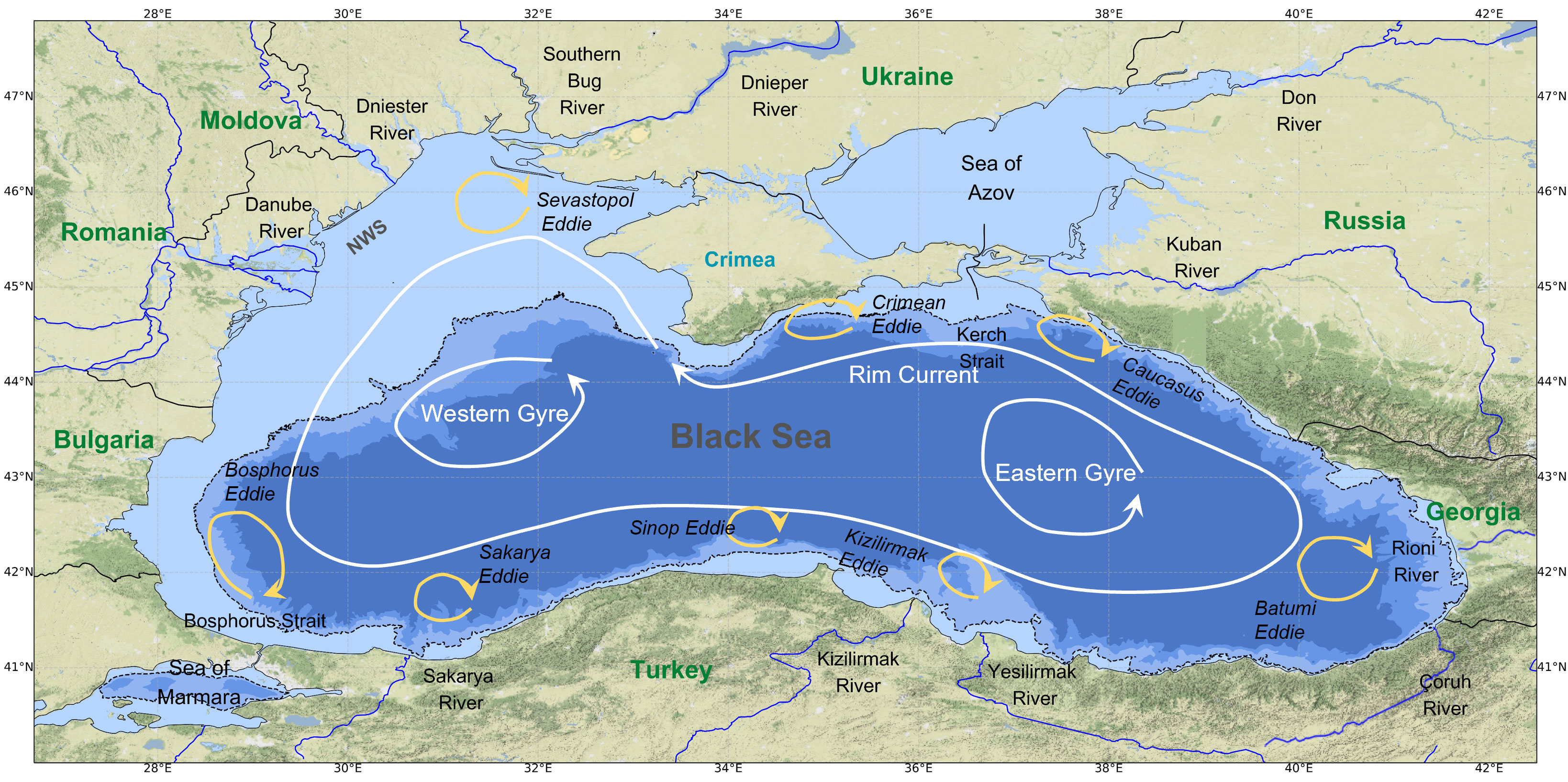
Figure 1 Map of the Black Sea with location of major rivers, North Western Shelf (NWS), the 200 m isobath (black dotted line), cyclonic gyres (white) and anticyclonic eddies (yellow). Made with data from Natural Earth and GEBCO, both licensed under Public Domain.

The results of FML numerical models, however, have sparked debate on how they should be configured to accurately replicate trajectories, particularly regarding the inclusion of wave effects through Stokes drift. Stokes drift is the net drift velocity experienced by a particle in the direction of wave propagation and is described as the difference between the mean Lagrangian velocity and Eulerian velocity of the fluid at the same depth (van den Bremer and Breivik, 2018). Previous studies suggest that the impact of Stokes drift on the transport and accumulation of FML may be prevalent under certain seasonal conditions and depending on the size scale of the floating elements, as well as the region being studied (Isobe et al., 2014; Iwasaki et al., 2017; Onink et al., 2019). More recently, Bosi et al. (2021) concluded that the inclusion of Stokes drift is necessary in particle tracking models of FML to avoid overestimating its residence time.

In the Black Sea, simulations have been conducted with and without the inclusion of Stokes drift. Miladinova et al. (2020) argued that the contribution of surface currents plays a more critical role in the accumulation of FML and therefore the inclusion of Stokes drift can be omitted in small element modeling. However, other simulations, such as those conducted by Stanev and Ricker (2019), have included Stokes drift and have found a clear linkage with FML accumulation on the southern coast. Both studies presented substantial differences in residence time, with an average beaching time of 200 days for simulations that did not include Stokes drift and 20 days with Stokes drift.

In a study conducted by Korshenko et al. (2020) in the coastal areas of the northeastern Black Sea, the discharge of floating marine litter (FML) from rivers was simulated. The results showed that approximately 46% of the discharged particles were washed ashore due to the influence of Stokes drift, while only 3.6% were observed without considering Stokes drift in the simulations. This finding indicates that surface wave-induced Stokes drift plays a significant role in the coastal pollution of FML, surpassing the impact of coastal currents.

There have also been discrepancies in the results regarding accumulation zones of FML. Miladinova et al. (2020) identified a retention zone in the western gyre during summer that moves to the east during winter, as well as a stable retention zone on the southwest coast that persists under different modeling conditions. In contrast, Stanev and Ricker (2019) research did not identify evidence of accumulation in open waters in their simulation for one year but they identified high concentrations of FML along the west and south coasts. Additionally, the data compiled by González-Fernández et al. (2022) show a high accumulation zone in open waters in the eastern basin, Odessa port, and northeastern zones. It is worth noting that the last study is limited by the lack of data in the southern and western zones of the Black Sea.

Other recent Lagrangian models applied more locally in the Black Sea have shown that the formation of circulation microstructures in coastal areas (Demetrashvili et al., 2022) and the seasonal variability of rivers (Yazir et al., 2022) are determinants of FML distribution patterns.

It is therefore suggested that there is a need for a more accurate model that can account for a wider range of processes affecting the spread of FML, particularly in coastal zones. Processes such as “beaching” or stranding, which refer to the interaction of FML with the shoreline, are relevant for identifying hot spots and developing strategies to clean up and mitigate the impact of FML pollution. As more data and research become available, it will be important to continue refining numerical models to improve predictions and develop effective solutions.

In this study, we use a numerical model of FML with a coastal emphasis to predict its transport in the Black Sea. Additionally, we evaluate the degree of agreement between our model predictions and the measurements and results reported by other authors. Dispersion and accumulation predictions with a basin model (Strokal et al., 2022) are performed to study the fate of the FML discharged by main rivers. Our objective is to bring a new perspective to current knowledge and to explore the hypothesis that Stokes drift plays a crucial role in the modeling of FML in the Black Sea. By doing so, we aim to contribute to a better understanding of the mechanisms that control the transport of FML in this region and provide valuable information for the development of effective management strategies. The paper is structured as follows: first, we present the marine litter model, the data used, and the methodology for validation and comparison experiments. This is followed by an analysis of results and discussion, and, finally, the conclusions are presented.

2 Materials and methods

This study utilized a coastal marine litter model known as LOCATE, which leverages OceanParcels (Delandmeter and van Sebille, 2019; van Sebille et al., 2020) as a Lagrangian solver. The model was developed by integrating Eulerian hydrodynamic data and Lagrangian simulations of marine litter particles. The main additional feature of LOCATE is that was developed to simulate specifically the motion and accumulation of litter particles in coastal areas, adapting to the use of nested grids of varying spatial scales and resolutions to account for coastal processes, and incorporating special modules like the beaching module. This model has been developed under the project of the same name (LOCATE: Prediction of pLastic hOt-spots in Coastal regions using sATellite derived plastic detection, cleaning data and numErical simulations in a coupled system) as a forecast and monitoring tool for areas of high accumulation of FML and consequently to improve regional management of FML in coastal areas. LOCATE has been applied on the coasts of the Mediterranean Sea (Trecchi, 2021; Hernandez et al., 2022), allowing the study of relevant processes in FML transport, such as beaching or ageing, that are still poorly understood. The adaptability of this model enables its use in various regions around the world, including the Black Sea basin.

2.1 Hydrodynamic numerical models

The configuration of LOCATE for the Black Sea is proposed with operational model data obtained from Copernicus Marine Service (CMEMS) developed for the Black Sea regional domain, and for this study, we only considered surface velocities. The hydrodynamic information is taken with a daily time resolution from the circulation model NEMO, v3.6 at 1/36° x 1/27° horizontal resolution. In terms of river runoff, a monthly climatological mean estimate is utilized as the inflow data. The circulation model NEMO takes into account a total of 72 rivers, including major ones (Lima et al., 2020). The Stokes drift data from the spectral wave model WAM Cycle 6 with a resolution of 1/36° x 1/27° and hourly time resolution (Staneva et al., 2022).

2.2 Lagrangian particles simulation

The OceanParcels Lagrangian solver allows LOCATE to simulate the motion of virtual plastic particles in space and time, based on the fundamental concept of applying the advection equation (van Sebille et al., 2018), which can be rewritten as a pathway equation after integrating both sides:

$\begin{array}{ll}\overrightarrow{x}(t)=\overrightarrow{x}(t_0)+{\int }_{t_o}^t\overrightarrow{u}(\overrightarrow{x},t),dt& (1)\end{array}$

where $\overrightarrow{x}$ is the three-dimensional position of a virtual plastic particle in space, t is the time and u($\overrightarrow{x}$,t) is the three-dimensional Eulerian flow velocity field, which includes the net current velocity and a wave induced drift. The location of a plastic particle at time $t$ depends on both the initial three-dimensional position of the particle and the velocity field $\overrightarrow{u}(\overrightarrow{x},t)$. The time evolution of a trajectory advected is solved numerically by a 4th order Runge-Kutta scheme. Note that $\overrightarrow{u}(\overrightarrow{x},t)$ is, by definition, a mean current and does not account for the particle dispersion induced by diffusivity at smaller temporal scales.

Therefore, diffusivity processes are incorporated into the model as stochastic and random displacement of particle positions as a function of the local eddy diffusivity (van Sebille et al., 2018). The time evolution of a stochastic process is solved by a stochastic differential equation (SDE), which includes the diffusivity tensor as a three-dimensional tensor incorporating the ocean/coastal diffusivity in the three-dimensional space. However, in OceanParcels only horizontal diffusivity vector can be simulated. We established the diffusivity parameter as a constant and then SDE can be simplified and integrated as:

$\begin{array}{ll}\overrightarrow{x}(t)=\overrightarrow{x}(t_0)+{\int }_{t_0}^t\overrightarrow{u}(\overrightarrow{x},t)dt+R\sqrt{\frac{2dtK}{r}}& (2)\end{array}$

where $R$ is a random process representing subgrid motion with a zero mean and variance $r$ =1/3, $K$ is the horizontal diffusion coefficient time and space invariant.

The value of $K$ is set to $10{\text{ m}}^2/\text{s}$ on the basis of the order of magnitude estimated from the literature on zonal and meridional absolute dispersion for the Black Sea (Bouzaiene et al., 2021; Ciliberti et al., 2022) and a previous sensitivity analysis concerning the standard deviations of the resulting trajectories at different values of $K$. Additionally, in order to identify and quantify the number of particles that reach the coast, including their stranding locations and arrival time, LOCATE incorporates the beaching module. This module detects the land-water boundary and updates the particle beached variable from 0 (indicating particles not beached) to 1 (indicating particles beached) when particles are deemed to have crossed the boundary. Subsequently, these beached particles are eliminated from the simulation, and their timestamp and coordinates are recorded for further analysis. It is worth noting that the consideration of particle re-suspension is not included.

As mentioned above, the particles used in this study are virtual tracers that do not possess mass, size, shape, or buoyancy. They are advected using surface flow field data of the Black Sea. In this assumption, no inertia is evaluated in their trajectories. It is important to note that by not considering mass or inertia, we do not account for processes such as degradation, fragmentation, clustering, or sinking that may influence the final amount and distribution of litter.

However, the use of Lagrangian models with virtual particles is a practical approach aimed at providing insights into the general patterns and most affected areas of litter dispersion. While the inherent properties and processes associated with litter, such as degradation and sinking, are beyond the scope of this study, it still offers valuable information about the overall behavior and distribution of litter in the Black Sea.

2.3 Model validation

The validation of a Lagrangian model such as LOCATE requires real dispersion data and final trajectories of elements moving on the surface in order to compare the reliability of the model. For this reason, it was decided to use data from drifters launched on the surface of the Black Sea. The dataset used (OGS - National Institute of Oceanography and Applied Geophysics Database) was taken by 5 satellite-tracked drifters deployed or recovered on the East Coast in 2008-2009. This zone was selected due to the previous information from literature about accumulation patterns. The type of drifters targeted are Coastal Ocean Dynamic Experiment (CODE); we discarded drifters with drogue at more than 1 m depth to exclude the influence of currents at depth and observe only the effect of surface currents and Stokes drift. The simulations were run with and without Stokes drift, releasing 100 particles every hour along the consecutive positions of the observed drifters with a prediction horizon of up to N = 72 h. The appropriate number of particles was determined after a sensitivity analysis of the standard deviation in the results of different simulations varying the number of particles.

The comparison of simulated and real trajectories was quantified through the Normalized Cumulative Lagrangian Separation (NCLS) distance and Skill Score (SS) (Liu and Weisberg, 2011). NCLS is the cumulative sum of the separation distance between simulated and observed trajectories D, weighted by the length of the observed trajectory accumulated over time L:

$\begin{array}{ll}NCLS=\frac{D}{L}=\frac{{\sum }_{i=1}^N{d}_i}{{\sum }_{i=1}^{N}l{o}_i}& (3)\end{array}$

$N$ is the forecast horizon, $l{o}_i$ is the length of the observed trajectory at time step $i$, and $d_i$ is the separation between the observed and simulated trajectories at that time step. It is worth noting that both the separation distance $d$ and the distance along the trajectory $lo$ in equation (3) accumulate over time. In contrast to other metrics, as the NCLS parameter is reduced, model performance improves, NCLS = 0 implies a perfect fit between observation and simulation. Meanwhile, SS is defined as follows:

$\begin{array}{ll}SS=\{\begin{array}{ll}1-\frac{NCLS}{n},\hfill & (NCLS\le n)\hfill \\ 0,\hfill & (NCLS>n)\hfill \end{array}& (4)\end{array}$

where $n$ is a tolerance threshold. It is a positive dimensionless number that determines the no skill criterion. In most cases, including ours, n is set to 1. However, it is possible to choose it heuristically (Sotillo et al., 2016; Révelard et al., 2021). In this metric, SS = 1 suggests that simulation and observation are exact matches.

All geodetic distances were calculated using the WGS-84 ellipsoid and the trajectory representing the results of each simulation is obtained as the average of the stochastic simulated particles. The hourly comparisons of the pairs of simulated and observed trajectories are then performed at time steps i … N, and the SS is computed as a function of N. The SS were compared at different prediction horizons (6H, 24H, 72H and 96H) and in two types -with and without Stokes drift, referred to as Stokes Drift (SD) and Non-Stokes Drift (NSD), respectively. These comparisons were made with the aim of evaluating the performance of the model over time and the differences regarding the use of Stokes drift. To determine the reliability of the model, a frequency analysis was conducted to obtain an overview of the measures of central tendency of the SS. [for more details, see (Liu and Weisberg, 2011; Révelard et al., 2021)].

2.4 Scenarios of particles input at the Black Sea

We defined two types of experiments with the aim to contrast with the results of existing Black Sea models, to assess the contribution of Stokes drift and to analyze the different accumulation patterns and their connection with the period and position of the release sites. In this regard, we selected hydrodynamic data from 2017 as they would allow us to compare our results with those of the models of Stanev and Ricker (2019); Miladinova et al. (2020) and observational data compiled by González-Fernández et al. (2022).

In the first homogeneous release scenario, our aim was to investigate the potential existence of accumulation patterns resulting solely from surface currents, seasonal behavioral variations, the identification of areas with the greatest concentration of marine litter, and the impact of incorporating Stokes drift. Furthermore, in the second, more realistic scenario, we conducted a particle release from the primary rivers using predictions from a river basin model (Strokal et al., 2022) to ascertain the direction, distribution, and ultimate fate of the released litter.

2.4.1 Homogeneous release

The initial simulation scenario involved the homogeneous release of 917 particles, which were uniformly distributed by placing one particle every seven nodes of the hydrodynamic data grid, thereby creating a grid with an approximate horizontal spatial resolution of 18 km (see Figure 2). The particle release took place at the beginning of each month over the course of 2017. Two distinct simulation types were conducted, one incorporating Stokes drift (SD) and the other excluding it (NSD), both with the beaching module activated.

FIGURE 2

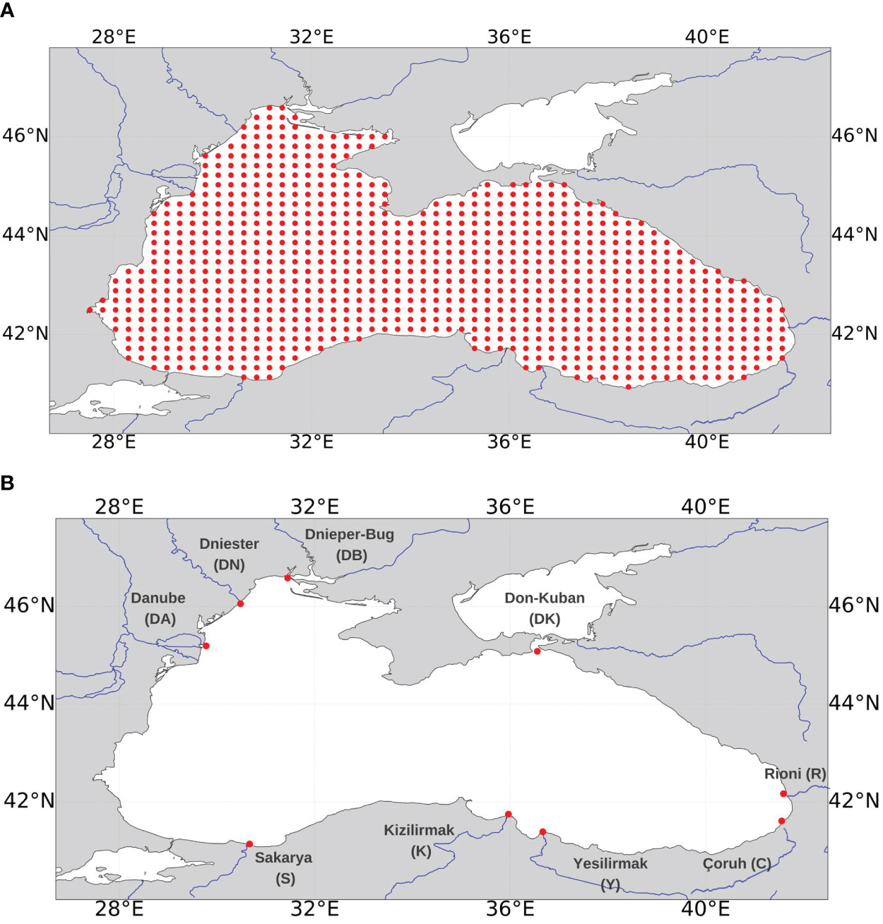
Figure 2 Graphical illustration of the simulation points used in the Black Sea particulate input scenarios. (A) Points distributed every 18 km ca. for the simulation case with homogeneous release. (B) Nine selected points with debris discharge from the main rivers of the Black Sea, named as follows: Dnieper-Bug (DB), Dniester (DN), Danube (DA), Sakarya (S), Kizilirmak (K), Yesilirmak (Y), Çoruh (C), Rioni (R), and Don-Kuban (DK).

2.4.2 Release from rivers

The second simulation scenario entailed the release of particles from the primary rivers that flow into the Black Sea, with selection criteria based on location and flow volume. The number of particles was estimated by calculating the average monthly flow of each river according to climatological data extracted from the Global Runoff Data Center (GRDC) database and model results provided in the Strokal et al. (2022) research on riverine export of microplastics for the year 2010. Strokal et al. (2022) data show microplastics river export in kt/year. Their river information is divided into five river groups: the Danube River, the Dnieper River, the Don River, the southern rivers and a total for all rivers.

We selected the 11 main Black Sea rivers and assigned to each of the three major rivers (Danube, Dnieper and Don) the corresponding number of kt/year according to the data. On the other hand, we distributed the number of kt/year of the southern rivers among the Sakarya, Kizilirmak, Yesilirmak, Çoruh and Rioni rivers in proportion to their total annual flow. In addition, we subtracted the kt/year of the above rivers already allocated from the kt/year exported by all rivers and this value was also distributed proportionally among the Bug, Kuban and Dniester rivers. In order to define the outflow points, some rivers such as the Dnieper and the Bug were joined at a single point due to their convergence, as were the Don and the Kuban, whose outflow point was established at the exit of the Kerch Strait. The location of the points was assigned to the nearest node with available current and Stokes drift data. Thus, the 9 points finally selected are shown in Figure 2 and all data used in the Table 1.

TABLE 1

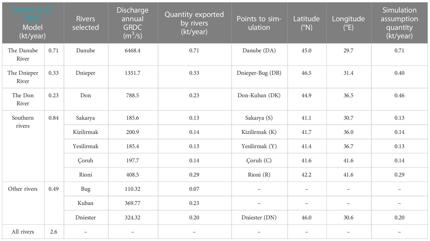
Table 1 Amount of plastics exported by the main Black Sea rivers (kt/year) according to Strokal et al., 2022, annual discharge data (m³/s) according to Global Runoff Data Center (GRDC) data, location of selected discharge points (longitude in °E and latitude in °N) and amount of plastic exported by each point assumed for the simulation (kt/year).

The simulation was set up with a continuous daily particle release. The number of particles was computed by the above extrapolation of the annual amount of marine litter exported for each river and the average monthly flux, further divided by the number of days in the month. This amount in kt is converted to the number of particles by setting the equivalent of one particle as 200 kg of marine litter, thus the amount of particles modeled at each point is variable depending on the seasonality and the amount of exported litter (Figure 3). It is assumed that the data provided by the Strokal et al. (2022) model can be applied as a benchmark and the modeling is carried out for the whole of 2017, under the same hydrodynamic conditions, K and with the beaching module activated as in the previous scenario.

FIGURE 3

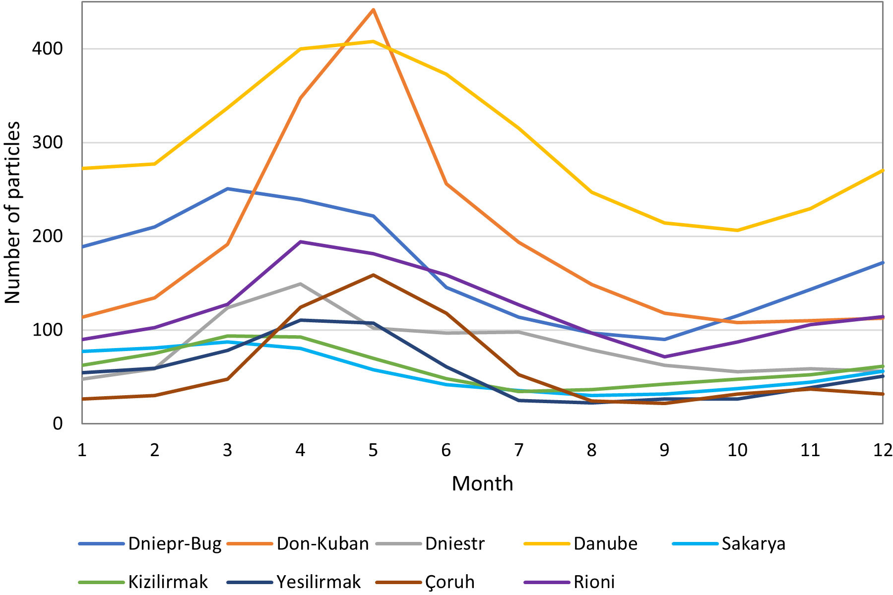
Figure 3 Number of particles released each month from the nine selected points, representing the amount of FML leaving each point for the simulation during the entire year 2017. This number of particles is estimated according to FML data taken from Strokal et al., 2022 and average annual discharge data taken from GRDC. Each particle represents 200 kg of FML.

3 Results

3.1 Validation of LOCATE for the Black Sea

The validation process involved a qualitative and quantitative comparison of simulated (sim) model trajectories and observed (obs) real trajectories. Figure 4 presents specific results for one of the selected drifters (drifter_3819), which was launched and recovered in the southwestern zone of the Black Sea, with a total travel time of 156 hours.

FIGURE 4

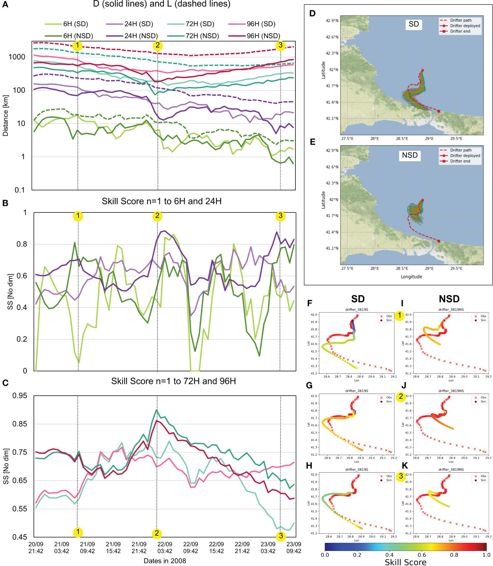
Figure 4 Time evolution of (A) cumulative separation distance D between simulated and observed trajectories (solid lines) and observed cumulative trajectory length L (dashed lines) (in logarithmic scale), (B) SS obtained using n=1 during the validation experiment with drifter 3819, after 6 h (green lines) and 24 h (purple lines), (C) SS obtained using n=1 during the validation experiment with drifter 3819, after 72 h (aquamarine green lines) and 96 h (red lines) of simulation. The intensity represents the type of experiment, light color for experiment without Stokes drift SD and dark color for experiment with Stokes drift NSD, (D, E) Representation of the trajectories resulting from the SD and NSD simulation from the same starting point of the drifter, (F–K) Spatiotemporal distribution of the resulting SS in the trajectories of the simulations with starting points at 1 2 and 3 along the drifter trajectory.

The Skill Score (SS), which evaluates the model, is calculated through the Normalized Cumulative Lagrangian Separation (NCLS) distance. The NCLS distance is the ratio of the accumulated sum of separation distances (D) over the accumulated sum of observed trajectory length (L). Figure 4A shows D and L for simulations with Stokes drift (SD) and without Stokes drift (NSD) for time horizons of 6, 24, 72, and 96 hours. For a 6-hour time horizon, D ranges from 1 to 18 km for the SD simulation and from 0.62 to 16 km for the NSD simulation. For a 24-hour horizon, the range of D is between 10 and 158 km for the SD simulation and between 5 and 122 km for NSD. For 72 hours, the range of D is between 141 and 784 km for SD and 73 and 489 km for NSD. Finally, for the 96-hour time horizon, the range of D is between 334 and 1150 km for SD and between 179 and 844 km for NSD. Smaller values of D result in higher SS, and vice versa, as seen in Figures 4B, C for the 6 and 24-hour time horizons, and for the 72 and 96-hour horizons, respectively. The highest peaks of SS are observed in NSD simulations, while minimum values are found in some SD simulations. These results differ from the qualitative appreciation initially observed in the images when performing simulations from the drifter launch point and for the total horizon of 156 hours, in which a better fit is observed in the SD simulation (Figure 4D) than in the NSD simulation (Figure 4E).

To further explain the reasons for the differences in SS values, three simulations with different starting points along the drifter trajectory (represented as 1, 2, and 3 in the Figure 4) were selected. The average trajectory and corresponding SS for SD and NSD are shown in Figures 4F–K, respectively.

For point 1 in SD simulation, D is nearly the same magnitude as L for the 6-hour time horizon, resulting in a low SS value of 0.11 (shown in blue in Figure 4F). SS increases to above 0.5 after 24 hours and reaches a value above 0.75 after 72 and96 hours. In contrast, for NSD, the SS is established above 0.6 in the first few hours and reaches 0.75 for the subsequent 72 and 62 hours. The highest peak of SS is 0.89 at a time horizon of 72 hours (point 2) in an NSD simulation; at this point another maximum SS is also observed at 96 hours (0.86), with subsequent values of 0.82 and 0.51 for 24 and 6 hours, respectively. In this case, an excellent fit with the drifter trajectory is observed during the evaluated hours, although a clear deviation is evident at the end of the trajectory for longer time horizons (Figure 4J). On the other hand, although the trajectory of the SD simulation behaves very similarly to that of the drifter over long distances, D appears to be sufficiently high in the first 6 hours, resulting in a decreased SS value of 0.44. For 24, 72, and 48 hours, this index exceeds a value of 0.67, but as it is a cumulative calculation, the significant difference in the first hours has an effect on the subsequent SS values, as expected.

In this regard, the results for this drifter show acceptable SS values for both NSD and SD simulations, although NSD simulations achieve higher values due to lower D values in the initial hours of simulation. Consequently, the total accumulated D is much lower for longer time horizons, even though they do not fit the observed trajectory very well (Figure 4K). In other words, SD type simulations are affected by greater differences in the initial hours, although they may have better fit at longer time horizons, as observed in point 3 represented in Figure 4H for SD and 4K for NSD.

Similar results are observed in the comparison of the results of other drifters. Figure 5 shows the SS results of the average trajectory compared to all the drifters selected with simulations carried out from the point of origin. The values of SS the total simulated trajectory of the five selected drifters from their actual point of origin were between 0.49 and 0.83 for SD type simulations and between 0.60 and 0.78 for NSD type simulations. The first two drifters show a better fit in the NSD type, but conversely, the last 3 show a better fit in the SD type. However, as explained above, despite the overall good qualitative agreement, the quantitative results for drifter 3819 present a discrepancy possibly due to large differences at the beginning of the trajectory. Although these results do not categorically affirm the use of Stokes drift, its influence can be observed, especially with long time horizons.

FIGURE 5

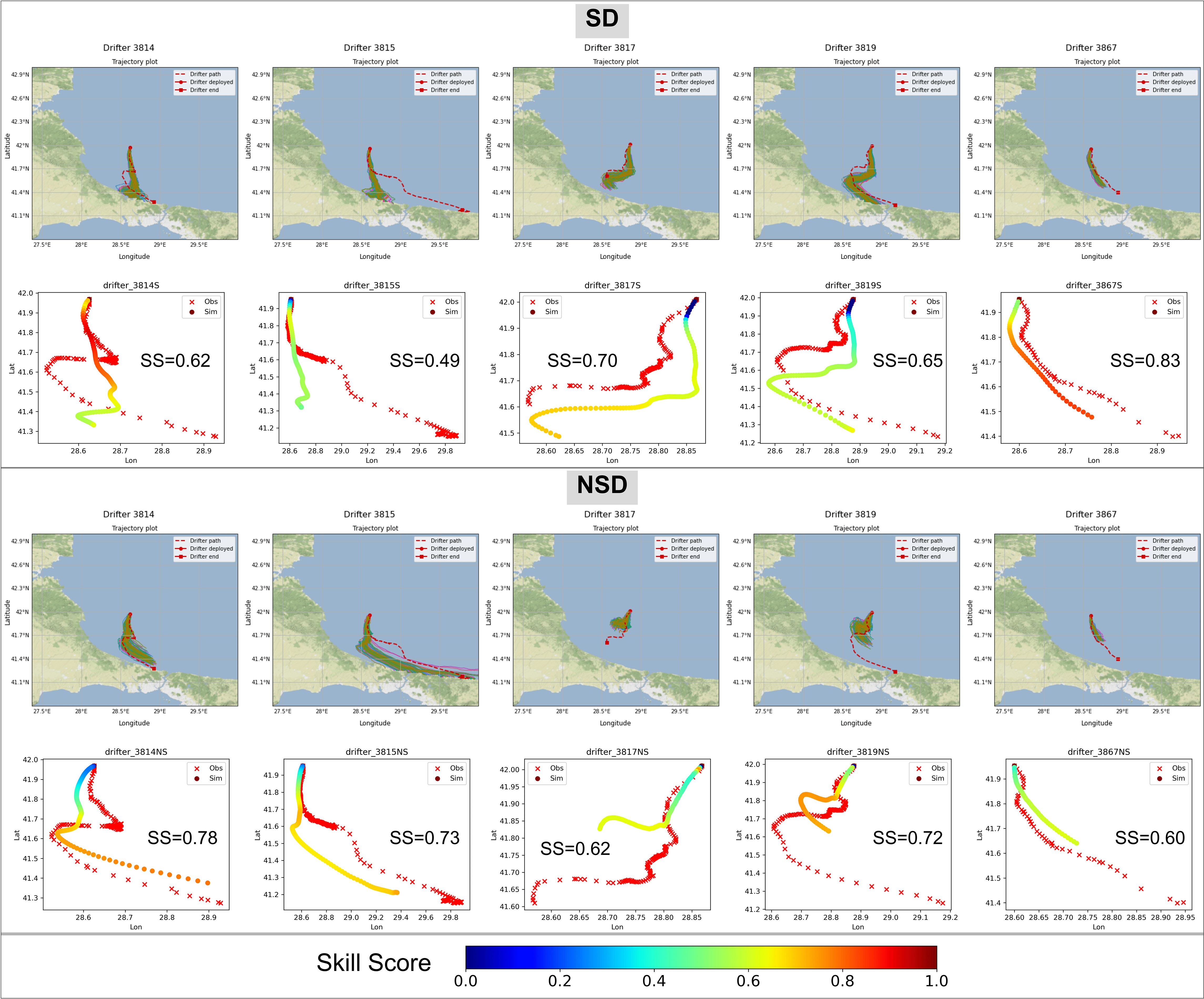
Figure 5 Graphical results of five drifter simulations from their points of origin and their resulting spatiotemporal distribution of SS in the trajectories of the simulations. Final Skill Score (SS) values for the total trajectory in each simulation are shown.

The final results of the SS evaluation for simulations are summarized in Figure 6 and Table 2, where the histograms for each of the time horizons and their measures of central tendency are shown. For the 6H horizon, the highest percentage of SS has low values (between 0 and 0.15) and a median of 0.267 for SD simulations and 0.363 for NSD. This trend continues for the 24H horizon, with a median of 0.518 for NSD simulations and 0.441 for SD. For the 72H and 96H horizons, the highest percentage of simulations is within the range of 0.60 and 0.75 for both SD and NSD. The median values for 72H correspond to 0.649 for NSD and 0.466 for SD; which differ very little from the medians for 96H (0.638 for NSD and 0.487 for SD). In the 96H histogram, a small percentage of SS with values greater than 0.75 can be observed, with SD being higher than NSD. The results indicate that the model presents a great sensitivity to different time horizons, showing a greater ability to predict extended time periods with acceptable SS values. This suggests that the model is suitable for predicting the motion of floating objects drifting in the Black Sea. In addition, the model’s better performance in long trajectories provides a good level of confidence in the modelling FML under real conditions, in which the travel time of an item can be higher than 72H.

FIGURE 6

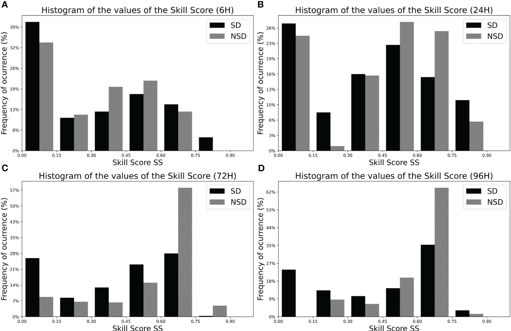
Figure 6 Histogram of Skill Score (SS) frequencies for the simulations performed for the validation of LOCATE in the Black Sea. The frequencies are provided for each time horizon (A) 6H time horizon, (B) 24H time horizon, (C) 72H time horizon and (D) 96H time horizon. The gray bars show results for NSD type simulation and the black bars for SD type simulation.

TABLE 2

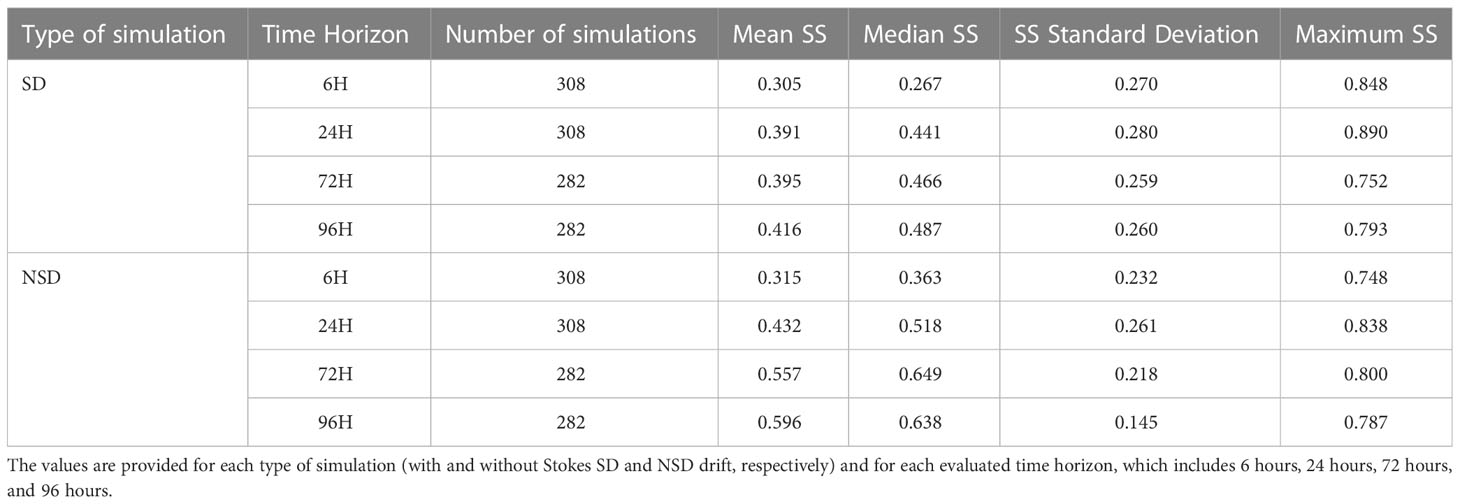
Table 2 Measures of central tendency for the Skill Score (SS) in the model validation simulations.

3.2 Accumulation patterns in homogeneous release

The homogeneous distribution of 917 particles released each month enabled us to observe their trajectories across the Black Sea and assess the impact of circulation dynamics. The simulation results were obtained by comparing the Surface Stokes Drift (SD) simulation, which incorporates the effects of Stokes drift, with the Non-Stokes Drift (NSD) simulation, which considers only the influence of currents. Particle density, defined as the number of particles per square kilometer, was calculated to evaluate particle accumulation at various locations, and the findings are presented in Figure 7.

FIGURE 7

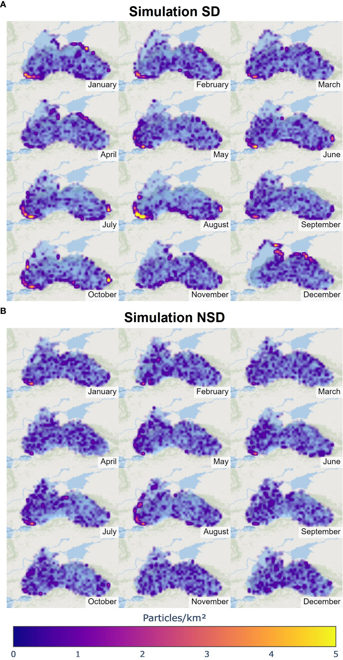
Figure 7 Particle density [particles/km²] resulting at the end of each month of 2017 with the simulation made with homogeneous particle release in experiments (A) (Top figure) SD (with Stokes drift) and (B) (Bottom figure) NSD (Non-Stokes drift).

In the SD simulation, the highest density of particles, 4,911 particles/km², was found in the southeast zone (SE) in October. The greatest density peaks (4 particles/km²) occurred in June in the southwest zone (SW) and in October in the SE. Subsequently, the months with high density values are February and August in the SW zone, with a wide high-density zone in the latter month and, in general, less dispersion in open waters and a slight accumulation trend along the entire south coast. The SE exhibited a small high-density zone in June, July, August and October. The average density value obtained in this simulation throughout the basin is 0.800, with a median of 0.749. In the NSD simulation, the maximum peak occurred in June in the SW, with a value of 3,973 particles/km². The highest values (3 particles/km²) were observed in June, July and January in the SW. As in the SD simulation, a wider area with high particle density was found in August. The average particle density throughout the basin was 0.744, with a median of 0.727.

In May, a high-density point is observed in the south, which may be connected to the presence of the Kizilirmak Eddy. In summer, anticyclonic activity intensifies, causing the formation of eddies between the Rim current and the continental edges. The formation of the western gyre, due to the breaking of the Rim current, continues to have an effect on the zone of high particle density on the western coast, leading to accumulation points further north. Furthermore, another high-density point is observed in the north during July and August, which may be associated with the formation of the Crimean Eddy. Finally, in October, the appearance of the Sakarya Eddy in the southwest and the Batumi Eddy in the southeast becomes evident, showing high particle density points in these locations. The results indicate that some points or zones of high particle density are directly related to circulation structures; significant accumulation trends were observed with both the NSD and SD simulation types in SW, particularly during summer months, and in SE in October. However, coastal accumulation is limited with the NSD simulation type and most particles remain in open waters, drifting within the basin. In this case, the influence of Stokes drift can be highlighted in the high particle density zones present in the northern part of the basin during the months of December and January, and in the high particle density zone in the SW in October, which has been contrasted with the wave field generated in these months with velocities between 0.2 and 0.3 m/s.

To perform a global assessment of the entire simulated year and accumulation trends throughout the basin, the region was divided into four quadrants: Northwest (NW), Southwest (SW), Northeast (NE), and Southeast (SE). We selected longitude 34.685°E and latitude 43.8°N as division limits. Figure 8 shows the resulting percentage of particles in each zone.

FIGURE 8

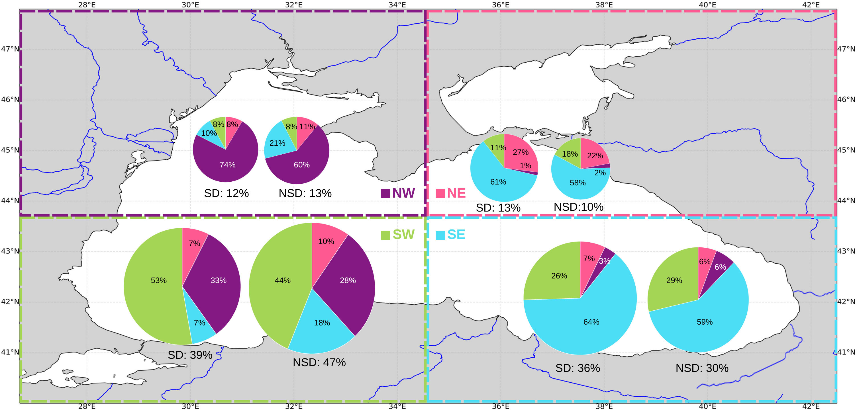
Figure 8 Distribution of total accumulated particles by quadrants according to their origin for the simulation of the whole year 2017. Pie charts are placed in the target quadrant and the colors indicate the origin, Southwest quadrant (SW) in green color, Northwest quadrant (NW) in purple color, Southeast quadrant (SE) in blue color and Northeast quadrant (NE) in magenta color. The percentages are shown in proportion to the size of the pie charts for each type of simulation. Left pie chart for Stokes drift (SD) simulations and right for Non-Stokes drift (NSD) simulations.

The largest percentage of particles for both SD and NSD simulations was observed in the SW quadrant, with values of 39% and 47%, respectively. The next highest accumulation was found in the SE quadrant, with percentages of 36% for SD and 30% for NSD. In contrast, the NW and NE quadrants showed a lower particle count at the end of the evaluation period.

Regarding the origin of the particles, the greatest percentage of particles in the NW, SW, and SE zones came from the same zone. However, in the NE quadrant, the largest percentage came from the SE quadrant. In the SW quadrant, approximately half of the particles originated from the same quadrant, while close to 30% came from the NW zone. These particles appeared not to travel in large numbers to the SE and NE quadrants.

A final analysis was conducted on the percentage of particles beached on shore for each simulation, along with the maximum and average minimum travel times and the average distance travelled (Table 3). It is observed that particles originating from the NE quadrant had a greater average distance travelled, consistent with their distribution across all quadrants as observed in Figure 8. Furthermore, the beaching percentage was noticeably higher for the SD simulation (75.5%) compared to the NSD simulation (45.5%). This discrepancy can be attributed to the NSD having fewer accumulation zones on the coast and a larger number of suspended particles throughout the basin. As a result, the average beaching time was also higher for the NSD simulation compared to the SD simulation.

TABLE 3

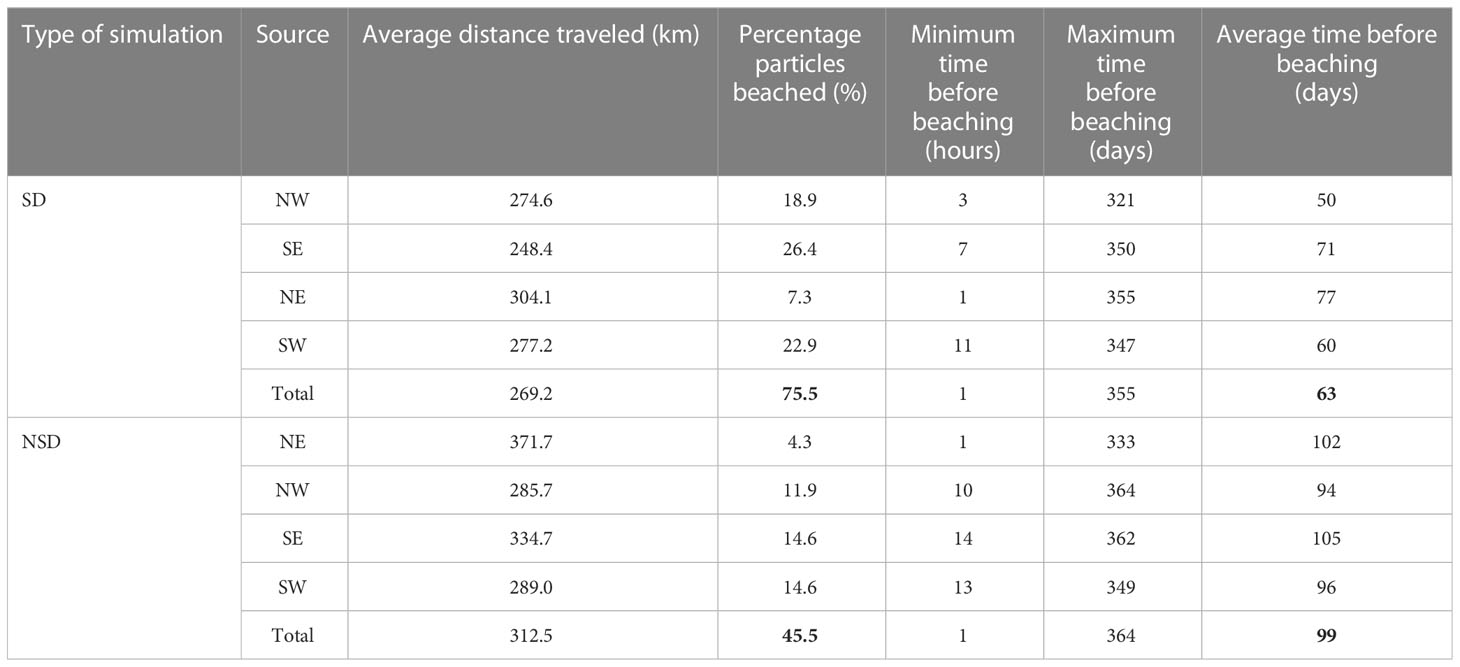
Table 3 Results of the analysis of the average distance traveled of particles [km], percentage of particles beached on shore (%), minimum [hours], maximum and average [days] beaching time for each type of simulation (with and without Stokes drift, SD and NSD respectively) according to their source quadrant.

It has been observed that, although numerical simulations incorporating Stokes drift (SD) or without incorporating it (NSD) show similar SS compared to drifts (with slightly higher SS for NSD), the inclusion of Stokes drift has a significant influence on particle accumulation in the coastal region and stranding. The simulations in the following section will be presented only with the inclusion of Stokes drift. A more detailed analysis will be presented in the discussion section.

3.3 Accumulation patterns in release from rivers

Figure 9 gives an overview of the trajectories resulting from the simulation of continuous release of particulate matter for one year at each of the 9 selected points located at the mouths of the most significant rivers. Particles from the Dnieper-Bug (DB), Dniester (DN) and Danube (DA) rivers tend to stay in the western part of the Black Sea, having mainly a movement from north to south. Particles from the Sakarya (S) move in an easterly direction and disperse mostly in the eastern part of the basin. On the other hand, the particles coming from Kizilirmak (K) and Yesilirmak (Y) tend to stay in the eastern part of the basin moving from south to north following the cyclonic circulation. Lastly, there is a greater movement from east to west of the particles coming from Çoruh (C), Rioni (R) and Don-Kuban (DK), the latter being the most dispersed throughout the basin.

FIGURE 9

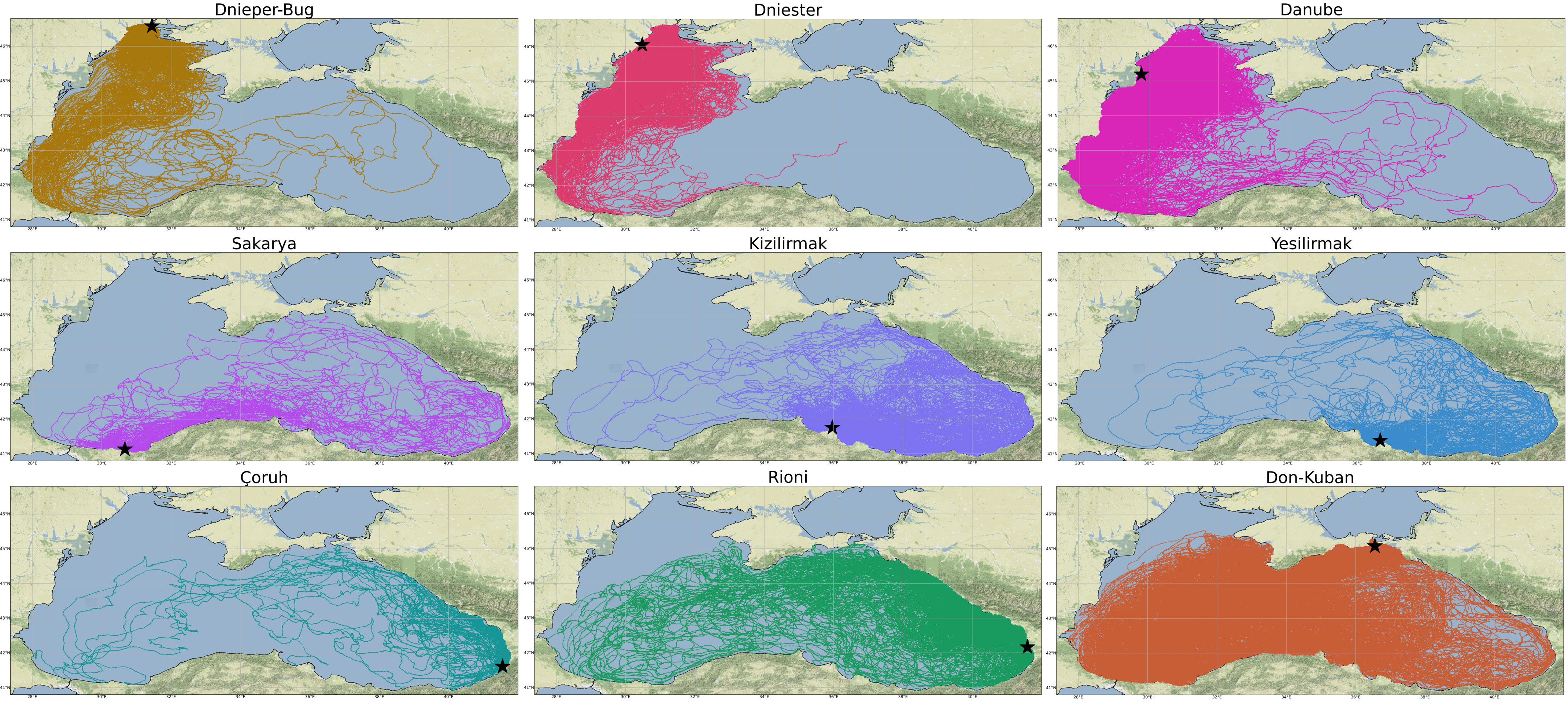
Figure 9 Final simulation trajectories for the entire year with particle release from each of the 9 selected points. Dnieper-Bug (DB), Dniester (DN), Danube (DA), Sakarya (S), Kizilirmak (K), Yesilirmak (Y), Çoruh (Ç), Rioni (R) and Don-Kuban (DK). The point of origin is indicated by a black star.

We also used the calculation of particle density to evaluate the accumulation trends for each month. In this case it was normalized with respect to the number of particles due to the monthly variation of incoming particles. The results of this analysis are presented in Figure 10. The highest particle density value of 0.023 particles/${\text{km}}^2$was observed in November in the area surrounding the DA river mouth. Peaks in particle density were also observed near the DN river mouth in September and near the DK point in April, with values exceeding 0.020 particles/${\text{km}}^2$.

FIGURE 10

Figure 10 Particle density [particles/km²] resulting at the end of each month of 2017 with the simulation made with particle release from 9 major FML discharge points associated with rivers.

In addition to the high particle density points that can be seen as discharge points, the results also reveal a significant accumulation of floating marine debris on the southwestern (SW) coast from January to August. This finding is likely due to the contribution of particles from the three northwest rivers and the DK, all of which flow into this region. Furthermore, the simulation revealed an accumulation in the northeast (NE) in November and a northwest (NW) accumulation in December.

An assessment of the cumulative particle distribution for the entire year was conducted by dividing the pie charts by discharge point into four quadrants: NW, SE, SW, and NE. The results show that the largest number of particles is accumulated in the NW quadrant with a percentage of 39%, followed by the SE quadrant with 37%, and the lowest percentage of particles in the NE quadrant with 14%. Moreover, within the NW zone, the majority of the particles originate from the Dnieper-Bug (DB), Dniester (DN), and Danube (DA) discharge points, with a small percentage coming from the Don-Kuban (DK) point. Moreover, 33.11% of the particles released by the DA, almost one third, end up in the SW area. In the SW zone, particles have more diverse origins, with the majority originating from the DA discharge point, followed by Sakarya (S) which is located within this quadrant, and 14% originating from DK. In the SE zone, particles mainly originate from the discharge points located within the same quadrant, including Kizilirmak (K), Yesilirmak (Y), Çoruh (C), and Rioni (R), with a small percentage originating from DK, which seems to be distributed throughout the basin, as seen in Figure 11. Furthermore, particles from R discharge point and the DK point account for most of the particles in the NE quadrant.

FIGURE 11

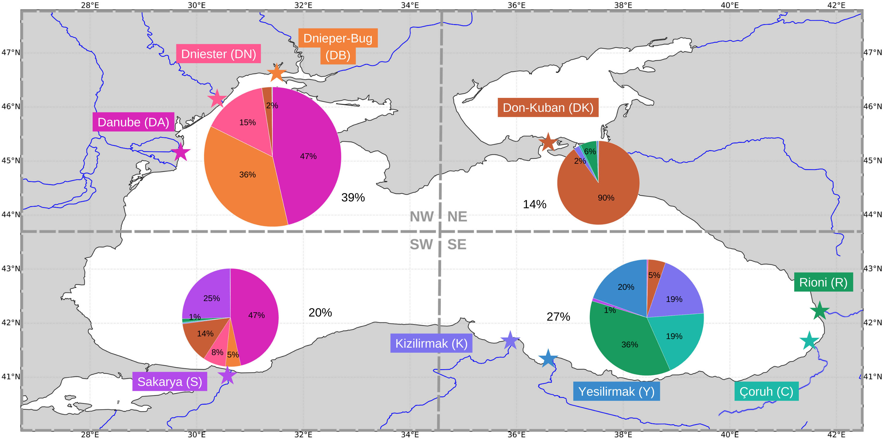
Figure 11 Distribution of accumulated particles by quadrants according to their origin for the simulation of the whole year 2017. Pie charts are placed in the target quadrant, Southwest quadrant (SW), Northwest quadrant (NW), Southeast quadrant (SE) and Northeast quadrant (NE). The colors indicate the point of origin which is marked with a star of the same color, Dnieper-Bug (DB) in orange, Dniester (DN) in pink, Danube (DA) in magenta, Sakaraya (S) in purple, Kizilirmak (K) in lavender blue, Yesilirmak (Y) in blue, Çoruh (Ç) in aquamarine green, Rioni (R) in green, and Don-Kuban (DK) in brown. The size of the pie charts are shown in proportion to the percentages.

Regarding the beaching analysis (Table 4), the results show a high percentage of particles that have beached on the coast, with an average of 92.6%. Among the studied particles, the DB particles have the highest percentage of beached particles, while K and DK particles have the lowest. The average distance traveled by the particles supports the previous findings, with the DK particles having the greatest distance traveled. On the other hand, particles from Y, S, and DB traveled the shortest distance. The average time before settling was 23 days, with values ranging from 12 to 14 days for Y, S, and DB, and 30 days for DK.

TABLE 4

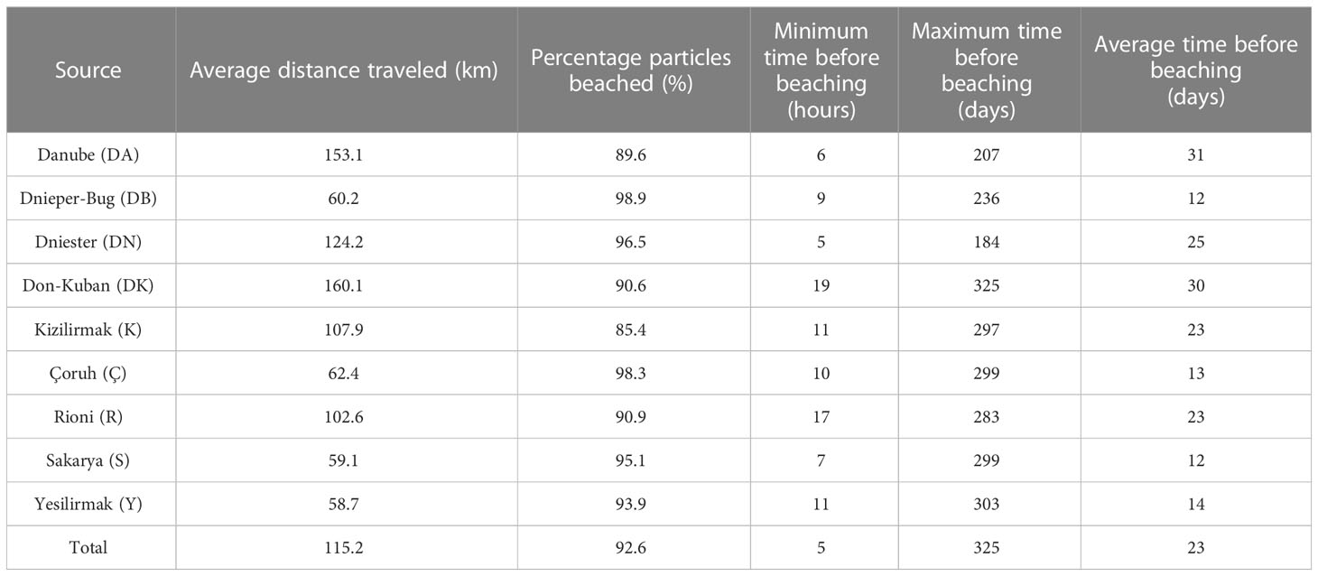
Table 4 Results of the analysis of the average distance traveled by the particles [km], percentage of particles beached on shore (%), minimum [hours], maximum and average [days] of beaching according to their point of origin.

4 Discussion

4.1 Stokes drift in FML modeling in the Black Sea

This study discusses the importance of considering Stokes drift in a numerical model for the transport of FML in the Black Sea. The evaluation was carried out in both the model validation and in the experiment with a homogeneous distribution of particles throughout the basin. During the validation of the results, it was observed that the experiment without including Stokes drift (NSD) generally has higher SS values, but this may be caused by the large differences during the first few hours in SD simulations, which has a cumulative effect on the final SS value. However, qualitatively, a good agreement was observed in the SD simulations regarding the determination of the final destination for two out of the three buoys used.

These results do not provide a definitive answer for or against the role of Stokes drift in FML transport, as factors such as buoy shape, size, and buoyancy must be considered. Additionally, buoy experiments typically do not cover near shore areas as the drifters are removed before reaching the shore. Therefore, the way Stokes drift affects these buoys may differ significantly from its impact on FML transport. Laboratory experiments have observed the effect of wave-induced motion on FML transport, which demonstrates that floating particles move with the Stokes drift velocity, and their size and density do not affect their movement (Alsina et al., 2020).

Regarding the experiment with a homogeneous particle release, it was observed that the inclusion of Stokes drift has an influence on the accumulation of particles on the coast, showing high accumulation points in the NW, NE, and SE zones during certain months of the year in the SD simulation that are not evident in the NSD simulation. For example, a trend of accumulation towards the SE area between the Çoruh and Rioni rivers can be observed from June to October in the SD simulation. In the NSD simulation, this point is only observed in October. From December to April, in the SD simulation, there is an accumulation zone in the NE area near the Russian coast and the Kerch Strait, and in December, an accumulation zone was observed on the NW coast of Crimea. The transport of FML towards these areas has been evidenced by several studies of beach litter collection and vessel-based surveys that identify among their results litter of foreign origin in different months and seasons (Topçu et al., 2013; Suaria et al., 2015; Aytan et al., 2019; Machitadze et al., 2020; Todorova et al., 2021), thus demonstrating that the simulation with NSD does not truthfully represent the transport to these areas.

Furthermore, a difference of 30% more particles being beached was found when the velocity contributed by Stokes drift was included, which is in agreement with the observations of Korshenko et al. (2020) in his simulations. In contrast, the average residence times were reduced by almost 36% (from 99 to 63 days) in the SD simulation, which is consistent with what other authors have observed (Isobe et al., 2014; Iwasaki et al., 2017; Onink et al., 2019; Bosi et al., 2021) in terms of the impact on both temporal scales and concentration in the main accumulation zones and their seasonal prevalence.

In this sense, it is deemed relevant to consider the Stokes drift in the subsequent simulation of particle release from the river basin points. This is because the qualitative results obtained in homogeneous release simulation indicate that the SD simulation better represents the coastal accumulation of FML in some areas. Additionally, previous research has experimentally demonstrated the influence of Stokes drift on the transport of FML in coastal areas. It is worth noting that the beaching rates obtained from the Stokes drift simulation are consistent with those from previous studies on beached FML (Dobler et al., 2019; Lebreton et al., 2019; Chenillat et al., 2021), particularly in experiments in semi enclosed basin areas (Carlson et al., 2017).

In summary, these observations aim to contribute to the discussion on the importance of Stokes drift in FML models for the Black Sea. This will ensure that these tools effectively guide prevention or cleanup actions, without overestimation in temporal terms or underestimation in terms of targeting sensitive accumulation zones.

4.2 Comparison with the results of previous models

Numerical models have been used in previous studies to investigate the accumulation patterns and average beaching time of the Black Sea, revealing differences in both coastal and open water. Next, the presented results are compared with those of Stanev and Ricker (2019) and Miladinova et al. (2020), who used different methodologies, including the implementation of Stokes drift and different models. They performed experiments with homogeneous scenarios and with particle release from hot spots.

In comparison to Stanev and Ricker (2019), homogeneous experiment with Stokes drift yielded similar results in January, with an accumulation zone observed in the southwest near the Bosphorus Strait and in the northeast on the Russian coast. In July, agreement was reached on the western coast, but higher concentrations were observed in areas further south in the Bosphorus Strait. A high accumulation point was also identified in the coastal zone between Georgia and Turkey, which was not observed in the work of Stanev and Ricker (2019), despite an agreement in the southeast zone. The low or zero-density particle zones agreed in Stanev and Ricker (2019) study, such as in January in the northeast zone and in July in the northeast and central-south zones.

In comparison to Miladinova et al. (2020) in their homogeneous experiment without Stokes drift, higher concentrations were agreed on the northeast on the North Western Shelf (NWS) and southern coast of Crimea in April. However, an accumulation in the central-south zone was not observed in the results. In

July, some small areas of the southwestern coast and the coastal zone between Georgia and Turkey were agreed upon, but no agreement was found on the accumulation in the northeast zone shown by Miladinova et al. (2020), nor in the southwest zone observed.

Findings regarding particle movement along the coast were consistent with those of Stanev and Ricker (2019) simulations, where particles were released from the eight major discharge points. In both studies, high-density areas were observed around the mouths of rivers. In particular, the northwest coast near the mouth of the Danube was identified as the area with the highest concentration of stranded particles. This observation was also reported by Miladinova et al. (2020), who similarly showed accumulation in this area. All three studies, including this study, agree that the accumulation of particulate matter along the coast is governed primarily by cyclonic circulation.

In the results of the most realistic scenario of FML release from rivers, there was no evidence of a large concentration of particles in open water for most months. In December, some dispersion is observed in the northwest area of the NWS, but due to the limited duration of the exercise, it is uncertain whether this dispersion will persist over time. Given the low average beaching time and the distance to the coast, it is expected that these particles will tend to move towards the shore. These findings are in line with those presented by Stanev and Ricker (2019) and are different to the results reported by Miladinova et al. (2020), who observed open water accumulation of FML predominantly in the western gyre during summer.

Another point of contrast is the average beaching time. The results obtained in the present study (≈ 33 days) are more similar in magnitude to those presented by Stanev and Ricker (2019) (≈ 20 days), but they are far from those obtained by Miladinova et al. (2020) (≈ 200 days) and are related to the high rate of beached particles and the resulting low number of particles in open water.

In general, the results showed agreement with Stanev and Ricker (2019) regarding accumulation patterns in the west and southwest zones, as well as the magnitude of the average beaching time. However, there was more accumulation observed in the southeast zone than in the southwest in the experiment with release from the rivers, which differed from Stanev and Ricker (2019) results. On the other hand, the findings aligned with Miladinova et al. (2020) results in the increasing accumulation observed over the NWS and shelf break due to the large number of particles leaving from surrounding discharge points, which generally continued into the summer months. Another point of agreement among the three studies was the existence of high concentration zones along the southeast coast.

4.3 Comparison with measurements data

The simulation results, which are based on FML export data from nine main discharge points with continuous particle input, reveal an average density of 0.0027 particles/km². The average mass of FML was estimated to be approximately 0.54 kg/km² based on the assigned release data in the LOCATE FML model, which assumes a mass value of 200 kg for each virtual particle. Using a typical weight for a plastic bottle of 10 g, the estimated density of FML is about 54 bottles per km² on average. However, it should be noted that this method provides a rough estimate based on a single type of item and is only used for the purpose of comparing results with previously reported data based on direct observations. The actual number of items per km² may vary depending on factors such as the type of FML, its size, or state of fragmentation.

Early research on FML was mainly focused on coastal waters. BSC (2007) reported average density values of 6.6 and 65.7 items/km² for the Ukrainian coast and the Kerch Strait, respectively, in a survey conducted in 2003. The simulation results in this study showed estimated values of 51.15 items/km² for one point in Ukrainian coast and 430.7 items/km² for one point in Kerch Strait. In the northwestern zone of the Black Sea, from the Danube Delta to the port of Constanta in Romanian waters, Suaria et al. (2015) estimated an average density of 30.9 items/km² with a peak of 135.9 items/km² at the mouth of the Danube. However, simulation results reveal a higher estimated density of 456.6 items/km² at this location, which is the highest point in the findings.

Subsequently, Machitadze et al. (2020) reported observations in Georgian territorial waters, with transects spanning from Batumi Port to Poti. The findings revealed average densities of 76.3 items/km², with a peak of 448 items/km² in the vicinity of the port of Poti. The authors proposed that the uniformity, type of items, material, and degradation state suggest a significant contribution of container ship waste. In comparison, simulation results indicate an estimated density of 59.37 items/km² this area. Furthermore, Berov and Klayn (2020) reported high densities of FML along the Bulgarian Black Sea coast, with a value of 93.8 items/km² observed west of Cape Kaliakra. The simulation results in this study also indicate high accumulation of FML in this area, with estimated values of up to 50 items/km² observed during the months of August and October. These findings align with the seasonal observations reported by Simeonova et al. (2017), which identified the highest quantities of FML during the summer period.

González-Fernández et al. (2022) recently reported fully compiled FML data in the Black Sea region from visual surveys conducted between May and November 2017, and June and October 2019. The simulation estimates an average density of 54 items/km² for the entire Black Sea, which is comparable to the weighted average density of 81.5 items/km² reported by González-Fernández et al. (2022). For the western basin, the study reported a weighted average density of 38.7 items/km², with a maximum of 581.3 items/km² in the Odessa region. In contrast, the simulation estimates an average density of 61.0 items/km² for the western basin, with the maximum point located at the mouth of the Danube and an estimated density of 89.7 items/km² in the Odessa region. It should be noted that this difference in estimated density could be due to data limitations in the western basin. In the eastern basin, González-Fernández et al. (2022) reported a weighted average density of 120.7 items/km², with a maximum of 810.2 items/km² in open waters more than 12 nautical miles from the coast. The simulation results suggest an average density of 46.0 items/km² for the eastern basin, with a maximum of 430.7 items/km² in the area surrounding the Kerch Strait. Notably, the simulation also identified high density points in the Anaklia and Batumi regions in Georgia coast, with values of 292.3 items/km² and 141 items/km², respectively.

Despite the simulation results not indicating significant accumulation of FML in open waters in the eastern basin of the Black Sea, regions with high FML pressure have been identified, such as Odessa in the northwest of Ukraine and the coastal area of Batumi in Georgia in the southeast, which agrees with González-Fernández et al. (2022). However, the simulation has certain limitations, such as being conducted for only one year and therefore may not accurately represent FML accumulation over longer periods. Furthermore, the spatial resolution of the simulation may not fully account for the accumulation of FML in anticyclonic eddies such as the Batumi Eddie or the Caucasus Eddie. In this sense, it would be beneficial to consider a model with a coastal approach and higher spatial resolution that could better represent local processes and account for inherent features of FML, such as its ability to be resuspended or beached in open waters. Such additions to the current model could improve its accuracy and enable a more comprehensive understanding of the accumulation of FML in the east basin.

5 Conclusions

The validation of the LOCATE Lagrangian FML model for the Black Sea was conducted using real drifter data and final trajectories of particles to assess the model’s reliability. The results suggest that while the use of Stokes drift is not categorically confirmed, its influence on FML transport can be observed, particularly at longer time horizons. Furthermore, the study found that the inclusion of Stokes drift significantly increased the time it takes for particles to wash up on shore, with NSD simulations resulting in longer beaching times than SD simulations. The experiment also demonstrated that the inclusion of Stokes drift has a significant impact on the accumulation of particles on the coast, with the SD simulation showing high accumulation points in the NW, NE, and SE zones during certain months of the year that are not evident in the NSD simulation. Additionally, the study found a 30% increase in the number of particles being beached when the velocity contributed by Stokes drift was included. Overall, these findings contribute to the discussion on the importance of considering Stokes drift in FML models for the Black Sea to guide effective prevention or cleanup actions.

In addition, this study provides valuable insights into the accumulation patterns of FML released from major rivers using estimated data of plastic exported from river basins into the Black Sea. The trajectories of particles from nine selected points were simulated for one year, revealing that particles from different rivers tend to stay in the vicinity of release points. The highest particle density value was observed near the Danube river mouth, and a long area of accumulation was extended over all the western coast. The northwest quadrant of the sea had the highest amount of accumulated particles, followed by the southeast quadrant, while the lowest percentage of particles was in the northeast quadrant. Furthermore, the beaching analysis showed a high percentage of particles that have washed up on the coast. The Dnieper-Bug particles had the highest percentage of beached particles, while the Kizilirmak and Don-Kuban particles had the lowest. Notably, the Don-Kuban particles had to travel the longest distance to reach the coast. In all scenarios, the southwest coast was identified as having high particle density.

The results of this study were compared with previous numerical models and field observation data, highlighting the crucial role of cyclonic circulation in governing the accumulation of FML on the coast, a conclusion consistent with prior research. However, this study also revealed some important differences from previous modeling studies, such as the identification of a high density point in the eastern region, off the coast of Georgia, and a notable presence of particles in the northwestern region, potentially linked to the influence of the three major rivers in the area. These findings based on recent observational data provide new insights into the complex dynamics of FML accumulation in the Black Sea.

Despite the limitations of the model discussed, such as the absence of the accumulation of FML present in open waters, this study opens the possibility of improving the model by adapting it to coastal regions with high resolution and considering the local dynamics and processes inherent to the accumulation of FML. The findings of this study can contribute to the generation of effective strategies to mitigate the problem of FML accumulation in the Black Sea. This study will be extended in future works with a much more detailed and shore-focused model, which will serve as a tool to guide prevention or cleanup actions in the Black Sea regions.

Data availability statement

The raw data supporting the conclusions of this article will be made available by the authors, without undue reservation.

Author contributions

LC-R, conceptualization, methodology formal analysis, investigation, writing – original draft, and visualization; IH, conceptualization, methodology, investigation, data curation, writing - review and editing; ME, conceptualization, methodology, resources, investigation, data curation, writing - review and editing, supervision and project administration. JA; conceptualization, methodology, resources, investigation, data curation, writing - review and editing, supervision and project administration. All authors contributed to the article and approved the submitted version.

Funding

The present study was developed within the DOORS European Union Project (Developing Optimal and Open Research Support for the Black Sea) project. This Project has received funding from the European Union’s Horizon 2020 research and innovation programe (Grant Agreement number: 101000518 — DOORS — H2020-BG-2018-2020/H2020-BG-2020-2).

Acknowledgments

The development of the presented model was initiated within the LOCATE (Prediction of plastic hot-spots in coastal regions using satellite derived plastic detection, cleaning data and numerical simulations in a coupled system) project funded by the European Spatial Agency ESA within the Open Space Innovation Platform (OSIP) campaign (Contract No. 4000131084/20/NL/GLC). L-CR acknowledges funding from Ministerio de Ciencia, Tecnología e Innovación de Colombia under Scholarship Program No. 885. IH acknowledges funding from Formació de Professorat Universitari (FPU-UPC 2020). JA acknowledges funding from the Serra Hunter programme.

Conflict of interest

The authors declare that the research was conducted in the absence of any commercial or financial relationships that could be construed as a potential conflict of interest.

Publisher’s note

All claims expressed in this article are solely those of the authors and do not necessarily represent those of their affiliated organizations, or those of the publisher, the editors and the reviewers. Any product that may be evaluated in this article, or claim that may be made by its manufacturer, is not guaranteed or endorsed by the publisher.

Abbreviations

FML, Floating Marine Liter; NWS, North Western Shelf; LOCATE, Prediction of pLastic hOt-spots in Coastal regions using sATellite derived plastic detection, cleaning data and numErical simulations in a coupled system; CMEMS, Copernicus Marine Service; SDE, Stochastic Differential Equation; OGS, National Institute of Oceanography and Applied Geophysics; CODE, Coastal Ocean Dynamic Experiment; NCLS, Normalized Cumulative Lagrangian Separation; SS, Skill Score; D, Accumulated sum of separation distances; L, Accumulated sum of observed trajectory length; SD, Stokes Drift simulation; NSD, Non-Stokes Drift simulation; GRDC, Global Runoff Data Center; SE, Southeast zone; SW, Southwest zone; NE, Northeast zone; NW, Northwest zone; DB, Dnieper-Bug; DN, Dniester; DA, Danube; S, Sakarya; K, Kizilirmak; Y, Yesilirmak; C, Çoruh; R, Rioni; DK, Don-Kuban.

References

Alsina J. M., Jongedijk C. E., van Sebille E. (2020). Laboratory measurements of the waveInduced motion of plastic particles: influence of wave period, plastic size and plastic density. J. Geophysical Research: Oceans 125, e2020JC016294. doi: 10.1029/2020JC016294

CrossRef Full Text | Google Scholar

Aytan U., Esensoy Sahin F. B., Karacan F. (2019). Beach litter on saraykoy¨ Beach (SE black sea): density, composition, possible sources and associated organisms. Turkish J. Fisheries Aquat. Sci. 20, 137–145. doi: 10.4194/1303-2712-v20206

CrossRef Full Text | Google Scholar

Aytan Ü., Pogojeva M., Simeonova A. (Eds.,) (2020). Marine Litter in the Black Sea. Turkish Marine Research Foundation (TUDAV), Publication No: 56, Istanbul, Turkey. 361 p.

Google Scholar

Berov D., Klayn S. (2020). Microplastics and floating litter pollution in Bulgarian Black Sea coastal waters. Mar. pollut. Bull. 156, 111225. doi: 10.1016/j.marpolbul.2020.111225

PubMed Abstract | CrossRef Full Text | Google Scholar

Bosi S., Broström G., Roquet F. (2021). The role of stokes drift in the dispersal of north atlantic surface marine debris. Front. Mar. Sci. 8. doi: 10.3389/fmars.2021.697430

CrossRef Full Text | Google Scholar

Bouzaiene M., Menna M., Elhmaidi D., Dilmahamod A. F., Poulain P. M. (2021). Spreading of lagrangian particles in the black sea: A comparison between drifters and a high-resolution ocean model. Remote Sens. 13, 2603. doi: 10.3390/rs13132603

CrossRef Full Text | Google Scholar

BSC (2007). Marine Litter in the Black Sea Region: A Review of the Problem (160Istambul, Turkey: Black Sea Commission Publications 2007-1).

Google Scholar

BSC (2019). State of the Environment of the Black Sea 2009-2014/5 (Istambul, Turkey: Publications of the Commission on the Protection of the Black Sea against Pollution (BSC).

Google Scholar

Carlson D. F., Suaria G., Aliani S., Fredj E., Fortibuoni T., Griffa A., et al. (2017). Combining litter observations with a regional ocean model to identify sources and sinks of floating debris in a semi-enclosed basin: the adriatic sea. Front. Mar. Sci. 4. doi: 10.3389/fmars.2017.00078

CrossRef Full Text | Google Scholar

Chenillat F., Huck T., Maes C., Grima N., Blanke B. (2021). Fate of floating plastic debris released along the coasts in a global ocean model. Mar. pollut. Bull. 165, 112116. doi: 10.1016/j.marpolbul.2021.112116

PubMed Abstract | CrossRef Full Text | Google Scholar

Chuturkova R., Simeonova A. (2021). Sources of marine litter along the Bulgarian Black Sea coast: Identification, scoring and contribution. Mar. pollut. Bull. 173, 113119. doi: 10.1016/j.marpolbul.2021.113119

PubMed Abstract | CrossRef Full Text | Google Scholar

Ciliberti S. A., Jansen E., Coppini G., Peneva E., Azevedo D., Causio S., et al. (2022). The black sea physics analysis and forecasting system within the framework of the copernicus marine service. J. Mar. Sci. Eng. 10, 48. doi: 10.3390/jmse10010048

CrossRef Full Text | Google Scholar

Delandmeter P., van Sebille E. (2019). The Parcels v2.0 Lagrangian framework: New field interpolation schemes. Geoscientific Model. Dev. 12, 3571–3584. doi: 10.5194/gmd-12-3571-2019

CrossRef Full Text | Google Scholar

Demetrashvili D., Bilashvili K., Machitadze N., Tsintsadze N., Gvakharia V., Gelashvili N., et al. (2022). Numerical modelling of marine litter distribution in Georgian coastal waters of the black sea. J. Environ. Prot. Ecol. 23(2), 531–541.

Google Scholar

Dobler D., Huck T., Maes C., Grima N., Blanke B., Martinez E., et al. (2019). Large impact of Stokes drift on the fate of surface floating debris in the South Indian Basin. Mar. pollut. Bull. 148, 202–209. doi: 10.1016/j.marpolbul.2019.07.057

PubMed Abstract | CrossRef Full Text | Google Scholar

González-Fernández D., Hanke G., Pogojeva M., Machitadze N., Kotelnikova Y., Tretiak I., et al. (2022). Floating marine macro litter in the Black Sea: Toward baselines for large scale assessment. Environ. pollut. 309, 119816. doi: 10.1016/j.envpol.2022.119816

PubMed Abstract | CrossRef Full Text | Google Scholar

Gunduz M., Özsoy E., Hordoir R. (2020). A model of Black Sea circulation with strait exchange, (2008-2018). Geoscientific Model. Dev. 13, 121–138. doi: 10.5194/gmd-13-121-2020

CrossRef Full Text | Google Scholar

Hernandez I., Espino M., Alsina J. M., Sánchez-Arcila A. (2022). Modelado numérico de la dispersión y acumulación de basura flotante en zonas costeras de la ciudad de Barcelona Type: Conference Poster in XVI Jornadas Españolas de Ingeniería de Costas y Puertos 2022.

Google Scholar

Isobe A., Kubo K., Tamura Y., Kako S., Nakashima E., Fujii N. (2014). Selective transport of microplastics and mesoplastics by drifting in coastal waters. Mar. pollut. Bull. 89, 324–330. doi: 10.1016/j.marpolbul.2014.09.041

PubMed Abstract | CrossRef Full Text | Google Scholar

Iwasaki S., Isobe A., Kako S., Uchida K., Tokai T. (2017). Fate of microplastics and mesoplastics carried by surface currents and wind waves: A numerical model approach in the Sea of Japan. Mar. pollut. Bull. 121, 85–96. doi: 10.1016/j.marpolbul.2017.05.057

PubMed Abstract | CrossRef Full Text | Google Scholar

Korshenko E., Zhurbas V., Osadchiev A., Belyakova P. (2020). Fate of river-borne floating litter during the flooding event in the northeastern part of the Black Sea in October 2018. Mar. pollut. Bull. 160, 111678. doi: 10.1016/j.marpolbul.2020.111678

PubMed Abstract | CrossRef Full Text | Google Scholar

Kubryakov A. A., Stanichny S. V. (2015). Seasonal and interannual variability of the Black Sea eddies and its dependence on characteristics of the large-scale circulation. Deep Sea Res. Part I: Oceanographic Res. Papers 97, 80–91. doi: 10.1016/j.dsr.2014.12.002

CrossRef Full Text | Google Scholar

Lazăr L. (2021). Impact of the rivers on the Black Sea ecosystem. Tech. Rep. 2.1 (CD PRESS), 225.

Google Scholar

Lebreton L., Egger M., Slat B. (2019). A global mass budget for positively buoyant macroplastic debris in the ocean. Sci. Rep. 9, 12922. doi: 10.1038/s41598-019-49413-5

PubMed Abstract | CrossRef Full Text | Google Scholar

Lechner A., Keckeis H., Lumesberger-Loisl F., Zens B., Krusch R., Tritthart M., et al. (2014). The Danube so colourful: A potpourri of plastic litter outnumbers fish larvae in Europe’s second largest river. Environ. pollut. 188, 177–181. doi: 10.1016/j.envpol.2014.02.006

PubMed Abstract | CrossRef Full Text | Google Scholar

Lima L., Aydogdu A., Escudier R., Masina S., Ciliberti S. A., Azevedo D., et al (2020). Black sea physical reanalysis (CMEMS BS-currents) (Version 1) dataset. Copernicus Monit. Environ. Mar. Service (CMEMS). doi: 10.25423/CMCC/BLKSEAMULTIYEARPHY007004

CrossRef Full Text | Google Scholar

Liu Y., Weisberg R. H. (2011). Evaluation of trajectory modeling in different dynamic regions using norMalized cumulative Lagrangian separation. J. Geophysical Research: Oceans 116, 1–13. doi: 10.1029/2010JC006837

CrossRef Full Text | Google Scholar

Machitadze N., Bilashvili K., Gvakharia V., Gelashvili N., Kuzanova I., Trapaidze V. (2020). “Analysis of the monitoring of the beach litter in the Georgia,” in Marine Litter in the Black Sea, vol. 56. (Istambul, Turkey: Turkish Marine Research Foundation (TUDAV), 37–48.

Google Scholar

Miladinova S., Macias D., Stips A., Garcia-Gorriz E. (2020). Identifying distribution and accumulation patterns of floating marine debris in the Black Sea. Mar. pollut. Bull. 153, 110964. doi: 10.1016/j.marpolbul.2020.110964

PubMed Abstract | CrossRef Full Text | Google Scholar

Onink V., Wichmann D., Delandmeter P., van Sebille E. (2019). The role of ekman currents, geostrophy, and stokes drift in the accumulation of floating microplastic. J. Geophysical Research: Oceans 124, 1474–1490. doi: 10.1029/2018JC014547

CrossRef Full Text | Google Scholar

Pogojeva M., Korshenko E., Osadchiev A. (2023). Riverine litter flux to the northeastern part of the black sea. J. Mar. Sci. Eng. 11, 105. doi: 10.3390/jmse11010105

CrossRef Full Text | Google Scholar

Révelard A., Reyes E., Mourre B., Hernandez-Carrasco,´ I., Rubio A., Lorente P., et al. (2021). Sensitivity of skill score metric to validate lagrangian simulations in coastal areas: recommendations for search and rescue applications. Front. Mar. Sci. 8. doi: 10.3389/fmars.2021.630388

CrossRef Full Text | Google Scholar

Simeonova A., Chuturkova R. (2019). Marine litter accumulation along the Bulgarian Black Sea coast: Categories and predominance. Waste Manage. 84, 182–193. doi: 10.1016/j.wasman.2018.11.001

CrossRef Full Text | Google Scholar

Simeonova A., Chuturkova R. (2020). Macroplastic distribution (Single-use plastics and some Fishing gear) from the northern to the southern Bulgarian Black Sea coast. Regional Stud. Mar. Sci. 37, 101329. doi: 10.1016/j.rsma.2020.101329

CrossRef Full Text | Google Scholar

Simeonova A., Chuturkova R., Yaneva V. (2017). Seasonal dynamics of marine litter along the Bulgarian Black Sea coast. Mar. pollut. Bull. 119, 110–118. doi: 10.1016/j.marpolbul.2017.03

PubMed Abstract | CrossRef Full Text | Google Scholar

Sotillo M. G., Amo-Baladrón A., Padorno E., Garcia-Ladona E., Orfila A., Rodríguez-Rubio P., et al. (2016). How is the surface Atlantic water inflow through the Gibraltar Strait forecasted? A lagrangian validation of operational oceanographic services in the Alboran Sea and the Western Mediterranean. Deep Sea Res. Part II: Topical Stud. Oceanography 133, 100–117. doi: 10.1016/j.dsr2.2016.05.020

CrossRef Full Text | Google Scholar

Stanev E. (2005). Understanding black sea dynamics: overview of recent numerical modeling. Oceanography 18, 56–75. doi: 10.5670/oceanog.2005.42

CrossRef Full Text | Google Scholar

Stanev E. V., Ricker M. (2019). The fate of marine litter in semi-enclosed seas: A case study of the black sea. Front. Mar. Sci. 6. doi: 10.3389/fmars.2019.00660

CrossRef Full Text | Google Scholar

Staneva J., Ricker M., Behrens A. (2022). Black sea waves reanalysis (CMEMS BS-waves, EAS4 system) (Version 1) dataset. Copernicus Monit. Environ. Mar. Service (CMEMS). doi: 10.25423/cmcc/blkseamultiyearwav007006eas4

CrossRef Full Text | Google Scholar

Strokal V., Kuiper E. J., Bak M. P., Vriend P., Wang M., van Wijnen J., et al. (2022). Future microplastics in the Black Sea: River exports and reduction options for zero pollution. Mar. pollut. Bull. 178, 113633. doi: 10.1016/j.marpolbul.2022.113633

PubMed Abstract | CrossRef Full Text | Google Scholar

Suaria G., Melinte-Dobrinescu M. C., Ion G., Aliani S. (2015). First observations on the abundance and composition of floating debris in the North-western Black Sea. Mar. Environ. Res. 107, 45–49. doi: 10.1016/j.marenvres.2015.03.011

PubMed Abstract | CrossRef Full Text | Google Scholar

Todorova V., Boicenco L., Denga Y., Tolun L., Tonay A. M., Oros A., et al. (2021). Black Sea monitoring and assessment guideline. ANEMONE Deliverable 1.3 (CD PRESS).

Google Scholar

Topçu E. N., Tonay A. M., Dede A., Öztürk A. A., Öztürk B. (2013). Origin and abundance of marine litter along sandy beaches of the Turkish Western Black Sea Coast. Mar. Environ. Res. 85, 21–28. doi: 10.1016/j.marenvres.2012.12.006

PubMed Abstract | CrossRef Full Text | Google Scholar

Trecchi D. (2021). Plastic debris dispersion on the Barcelona coast: a numerical study. UPC, Escola Tècnica Superior d'Enginyers de Camins, Canals i Ports de Barcelona, Departament d'Enginyeria Civil i Ambiental. Available at: http://hdl.handle.net/2117/362494 [Accessed August 1, 2023].

Google Scholar

van den Bremer T. S., Breivik O. (2018). Stokes drift. Philos. Trans. Ser. A Mathematical physical Eng. Sci. 376, 20170104. doi: 10.1098/rsta.2017.0104

CrossRef Full Text | Google Scholar

van Sebille E., Aliani S., Law K. L., Maximenko N., Alsina J. M., Bagaev A., et al. (2020). The physical oceanography of the transport of floating marine debris. Environ. Res. Lett. 15, 23003. doi: 10.1088/1748-9326/ab6d7d

CrossRef Full Text | Google Scholar

van Sebille E., Griffies S. M., Abernathey R., Adams T. P., Berloff P., Biastoch A., et al. (2018). Lagrangian ocean analysis: Fundamentals and practices. Ocean Model. 121, 49–75. doi: 10.1016/j.ocemod.2017.11.008

CrossRef Full Text | Google Scholar

Yazir D., Terzi Y., Eruz C. (2022). Transportation of microplastic during high-flow and low-flow seasons in southeastern Black Sea: A modelling approach. Indian J. Geo Mar. Sci. 51, 663–670. doi: 10.56042/ijms.v51i08.49207

CrossRef Full Text | Google Scholar