A new method for predicting the maximum wave height of ship-generated onshore slopes in restricted channel

1 Introduction

Riverbanks and coastal erosion have attracted much attention in recent years, and many investigators have focused on the effects of runoff, wind waves, and tidal movement on riverbank materials (Hofmann et al., 2008; Uncles et al., 2014; Williams et al., 2018). When a ship navigates in restricted waters, channel size, water depth, ship speed, and other factors directly influence the resistance to the ship and the angle of propagation of the ship-generated waves. Such factors are capable of increasing the resistance and remarkably altering the wave fluctuation process compared to non-restricted waters (Havelock, 1922; Noblesse et al., 2014; Li and Ellingsen, 2016; Du et al., 2020). However, with the quick development of shipping in restricted waters, the erosion and retreat of inland waterways and beaches have been substantially influenced by ship-induced waves, particularly the erosion of riverbanks and shallow areas of coasts (Nanson et al., 1994; Cameron and Bauer, 2014; Teatini et al., 2017). For confined channels or shallow coastal areas, erosion of beach slopes by ships and resuspension of suspended sand (Rapaglia et al., 2011; Mao and Chen, 2020), as well as on beach slope stability and wetland dispersal degradation, and disturbances of plants and animals and fish community habitats (Jägerbrand et al., 2019; Kurdistani et al., 2019).

By this virtue, some researchers have conducted investigations on riverbanks and coastal areas with high ship traffic flow (Fleit et al., 2021). It is essentially characterized by a shallow water area that has a negative influence on the survival and diversity of bottom prey organisms; as a general rule, the narrower the channel width, the greater the damage caused by the wave of boat traffic. For this type of waterway, the ability to dissipate the ship’s traveling wave energy is commonly weak, and after the ship passes the understudied surface, the wave collapse would be slow and causes erosion damage to the beach slope area of nearly 150 m. In addition to traditional current scouring, wave breaking also causes bed surface erosion (Bilkovic et al., 2019). Compared to wind-generated waves, ship-induced waves have a shorter period and higher peaks, so they commonly possess more energy and are identified as the main source of erosion in areas with low wind and wave energy (Stumbo, 2001; Safty and Marsooli, 2020). It is known that the energy of the ship’s wave in shallow water is more than the energy in deep water. Additionally, as the speed of the ship grows, the energy plot first exhibits an ascending trend and then a descending trend, indicating reaches a maximum at a certain speed. The height of the ship’s wave becomes greater when the energy is at its maximum level. The oscillation law and the propagation process of ship-generated waves in shallow coastal areas and restricted channels are dissimilar to the traditional water depth conditions of the wide area and exhibit some similarities (Scarpa et al., 2019). Hence, the maximum wave height is related to the maximum energy in the process of limiting water fluctuations and the degree of bank erosion, which can be reasonably utilized to estimate and predict the maximum energy of waves of traffic boats and riverbanks, as well as to judge the degree of coastal erosion. As a result, the explorations on predicting the maximum wave height of the ship-generated waves are of grave significance.

At present, because the ship-generated waves are irregular, the maximum wave height in the propagation path in the channel alters with a certain degree of randomness (Maynord, 2005). By utilizing the shipping speed, water depth, and ship type based on the actual measurement data for typical regression analysis, many investigators have established the prediction model of the maximum wave height of ship-generated waves, as the corresponding formulas are presented in Table 1. For this purpose, field experiments were employed to collect data to derive the maximum wave height equation for the beach under various ship speed conditions (Balanin and Bykov, 1965). Based on the Ohio River using observations of a specific vessel, a maximum wave height prediction formula is derived for ship-generated waves (U.S. Army Corps of Engineers, H.D, 1980); however, the aforementioned equation was developed for a specific type of ship orientation, which results from the measurement of the maximum wave height on the coast and the formation of a semi-empirical formula, with a strong regional and ship type restrictions, without taking into account the distance from the measurement point. In another work, (Bhowmik, 1975) collected the wave height generated by a ship at three distinct speeds and the formula for predicting the maximum wave height was then derived by regression analysis of the data, which was only applicable to low-speed cases on a low speed at that time. (Bhowmik et al., 1982) performed multiple regression analysis of significant parameters for 60 ships navigating the Mississippi River at speeds (0.98 m/s to 6.19 m/s) and wave measurement distances of 0.91 m/s to 213.36 m/s, which resulted in a linear correlation between H_m and ship speed (V_c). On this basis, we proceed to examine the maximum wave height produced by various ship types and ship speeds to obtain an exponential relationship between H_m and ship speed (V_c). The Permanent International Association of Navigation Congresses (PIANC) proposed a predictive equation model for channel lining design applicable only to ship waves generated by inland vessels (Pianc, 1987). (Sorensen, 1997) extracted the prediction curves of the maximum wave height of the ship-generated waves and the speed of the ship V_c by correcting the existing formulas; however, the aforementioned formulations for broader use conditions were not proposed. The above investigations all use field measurement data to fit the equation with multiple linear regression, which cannot accurately control the channel depth, ship speed, and measurement position. Among them, depth is one of the pivotal factors affecting the formation of the maximum wave height during the propagation of the ship-generated wave (Ozeren et al., 2016; Suprayogi et al., 2022). In addition, traditional predictive models employ traditional approaches such as least squares or Fmincon functions in nonlinear regression to fit multivariate equations, which are prone to locally optimal solutions in the fitting process (Paatero and Tapper, 1993), requiring the combination of new optimization algorithms in the parameter fitting part. Currently, the common optimization algorithms include genetic algorithm, simulated annealing, ant colony algorithm, and particle swarm algorithm (PSA). The PSA has the advantages of good convergence and easy separation from the local optimal solution compared to other ones.

TABLE 1

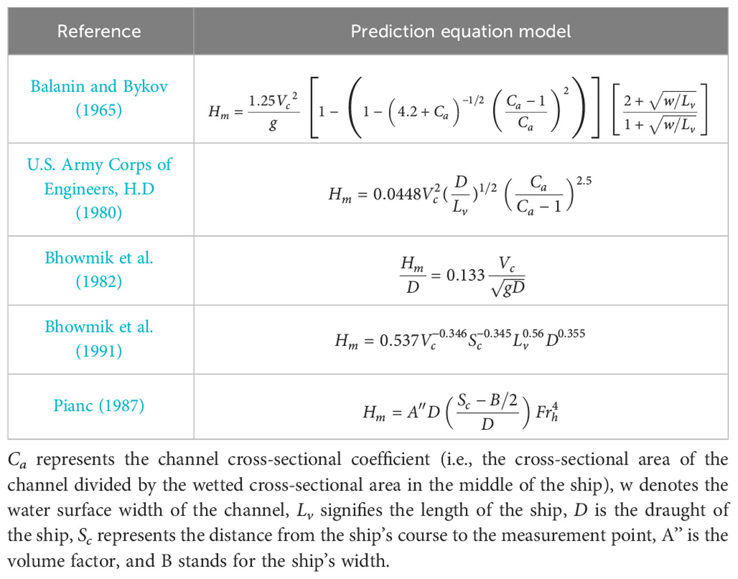
Table 1 Prediction equation models of maximum wave height (Sorensen, 1997).

With the rapid development of shipping, the types and sizes of ships gradually began to be unified. For a particular typical ship, its size and draft depth are no longer important factors that affect the change of the ship line’s wave height, but for confined waters, water depth and ship speed are among crucial factors that affect the maximum wave height of the ship’s line. Therefore, this paper is aimed to establish a physical model based on the cross-section of the common channel and the shape of the ship in confined waters. The proposed model is capable of measuring the distribution of the cross-sectional wave height under various conditions of water depth and ship speed using flume experiments. In continuing, an equation model dimensional analysis and particle swarm optimization algorithm (PSOA) is developed and established, seeking to solve the correlation coefficients based on the measured data. The final goal is to arrive at the equation model of the predicted maximum wave height of the ship-generated waves. In the present investigation, we construct a trapezoidal cross-section of confined water in a wide flume through adopting a laboratory experiment of our ship navigation test. Then, we proceed with determining the relationship between the maximum wave height, ship speed, channel water depth, and distance from the ship at the shore slope of shallower areas during the propagation of the ship-generated waves. The most crucial output is the development of a prediction formula via dimensional analysis and PSOA. The present article can be divided into four parts: the first part introduces the background of the study, the second part describes the experimental design and the methods used in the paper, the third part demonstrates the preliminary analysis of the experimental results and the discussion, and the fourth part provides a summary of the important results of the performed investigation.

2 Methods

The field measurement of the ship-generated waves is affected by the topography of the channel, water depth, frequency of ship traffic, and other factors, so it is difficult to obtain the water level fluctuation process data of the traveling wave in the presence of various water depths and ship speeds. The arrangement of the real-time collection points is also subject to great limitations, while laboratory flume experiments can be constructed according to the channel cross-section of the channel and ship model, the depth and speed of ships can be easily set up for the experiments, and the arrangement of the traveling wave measurement points is precisely arranged according to the content of the study. The arrangement of wave measurement points can be accurately arranged according to the research content. In addition, most of the traditional regression analyses use the least squares and Fmincon function methods, which are easy to fall into the local optimal solution and cannot scientifically obtain the form of a prediction equation. In order to build a maximum wave height prediction model for ship-generated waves in confined waters, this paper adopts laboratory flume experiments instead of field measurements. The main objective is to accurately control the measurement conditions and measurement positions of the wave gauge arrangement. Subsequently, we construct the prediction model through dimensional analysis and determine the correlation coefficients according to the PSOA, whose methods include the following three parts.

2.1 Laboratory flume experiments

The experiments were carried out in the Basic Sedimentation Theory Test Hall of Nanjing Hydraulic Research Institute. The experimental flume was a special tank for ship self-propulsion tests with the following dimensions: 30 m long, 5.0 m wide, and 0.5 m high. In order to appropriately examine the problem of the maximum wave height of the wave produced by the ship due to the navigation of the channel ship, the common domestic small and medium-sized channel sections are considered. Based on the ratio of 1:20, a trapezoidal cross-section structure is built in the flume, as demonstrated in Figure 1. The length of the experimental trapezoidal section is 10 m, which is located in the middle area of the water tank, before and after each of a 10 m buffer zone as a ship model acceleration and deceleration areas. To eliminate the impact of the reflection of the ship’s wave on the right bank velocity and wave height measurement, the experimental section on the right side of the channel model includes a ramp (1:3) to form a trapezoidal shore protection structure, and the left side is made of a 4–6 cm diameter gravel pile designed. Additionally, a large area of high-density vegetation network was placed before and after the flume to reduce the effect of water reflection on the experiment.

FIGURE 1

Figure 1 Schematic representation of the experimental flume arrangement.

The dimensions of the relevant sections in the flume model and the ship model have been presented in Figure 2. The trapezoidal section of the channel consists of two slopes with a slope ratio of 1:3, which are connected by a platform. The ship model employs the most common 500-ton cargo ship in the restricted channel as the research target, and the ship size is 46.0 m × 8.8 m × 3.0 m (length × width × draught) with a speed of 3.8 m/s to 11.2 m/s. Furthermore, according to the similar ratio, the size of the prototype ship is 2.30 m × 0.44 m × 0.15 m, and its speed is set as 0.85 m/s to 2.5 m/s. The ship model has auto-navigation power and can move itself by remote control. The ship’s rudder angle varies in the range of −25°–25°, and the ship’s navigation path in this study is taken as a straight line along the centerline of the channel.

FIGURE 2

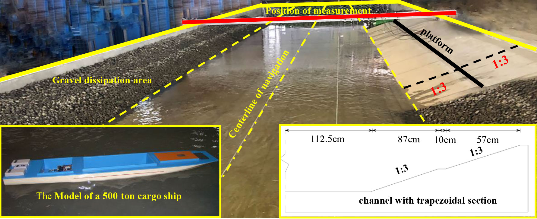
Figure 2 Actual production diagram of the flume and ship models.

This experiment employs three water depths (h_c) for testing, namely, 0.19 m, 0.29 m, and 0.39 m, and each water depth is used for conducting four ship speed tests. The ship navigation experiments should ensure that the water surface is calm before the ship is allowed to move in the center line of the channel, and the direction of navigation is set parallel to the riverbank. The self-propelled speed range of the ship is 1.06 m/s–1.68 m/s, because the restricted water is commonly divided into three regions according to the different propagation angles of the ship-generated waves. In the case of Fr_h ~0.84, the ship speed is placed in the subcritical speed region; for the case of 0.84 < Fr_h < 1.15, the ship speed is in the cross-critical speed region, while the case of Fr_h ≥ 1.15 is corresponding to the supercritical speed region. According to the experimental working conditions of water depth, the Froude number (Fr_h) is allowed to vary in the range of 0.54–1.2 to include all above velocity regions. The specific working conditions in the performed experiments are presented in Table 2.

TABLE 2

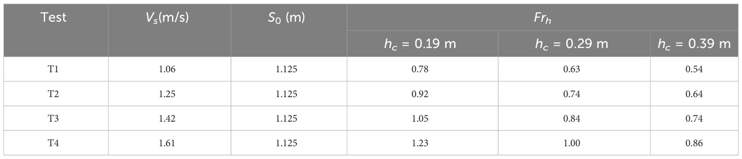
Table 2 Experimental condition group setting.

The wave height measurement in this experiment is performed by the 64-channel DS30 capacitive wave height measurement system and wave height meter, which uses electronic sensing and computer hardware-software technologies to simultaneously measure several points with high accuracy. The channel height meter arrangement is demonstrated in Figure 3, where the horizontal distance (S_c) from wave gauge 1 (W1) to the channel center gauge 10 (W10) is set as 0.865 m, 1.00 m, 1.225 m, 1.325 m, 1.350 m, 1.38 m, 1.580 m, 1.780 m, 2.090 m, and 2.370 m. Wave gauge 1 (W1) and wave gauge 2 (W2) are placed in the channel, and wave gauges 5 (W5)–10 (W10) are located on the channel slope (see Figure 3). The sampling frequency of the wave height meter is set equal to 100 Hz, and the acquisition time is set as 90 s, with a total of 9,000 data.

FIGURE 3

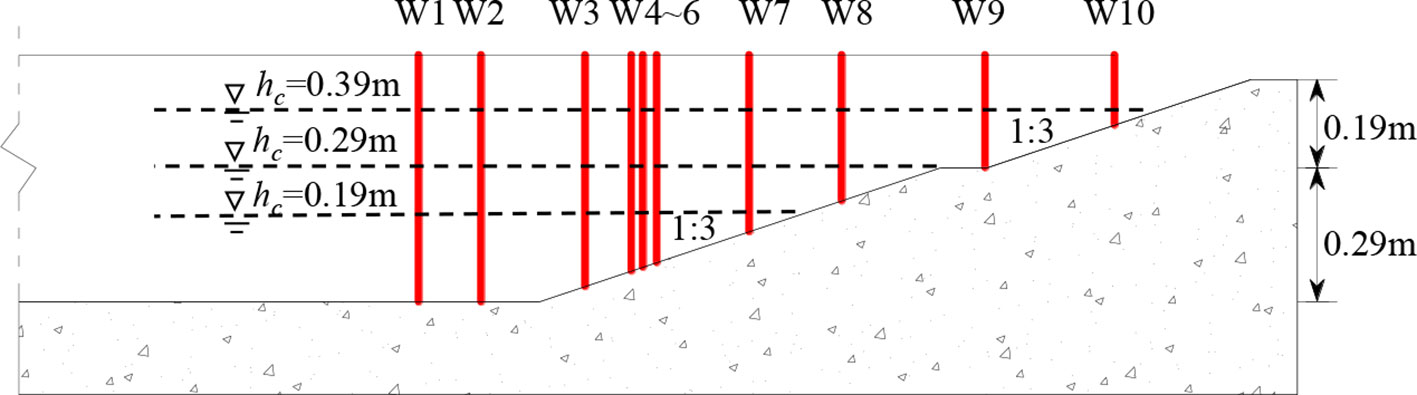
Figure 3 Schematic representation of the wave gauge layout.

2.2 Dimensionless analysis

Numerical analysis is aimed at providing a fairly accurate realization of the physical quantities involved in a physical problem and seeks to establish functional relationships between these quantities. That is a simplification of a physical problem in the context of analyzing the nature of the physical problem at the level of magnitudes. The theoretical basis of dimensionless analysis is the Buckingham π-theorem (Buckingham, 1914), which assumes the existence of n main influencing factors for a general physical problem. Generally, it can be stated by the following:

$\begin{array}{ll}Y=f\left(X_1,X_1,···,X_n\right)& \text{(1-1)}\end{array}$

By choosing m (m ⩽ 7) of these physical measures as basic measures, let us make up n–m dimensionless measures (${\prod }_1$, ${\prod }_1$,…, ${\prod }_{n-m}$). Then, one can write:

$\begin{array}{ll}f\left({\prod }_1,{\prod }_1,···,{\prod }_{n-m};\prod \right)=0& \text{(1-2)}\end{array}$

The inland waterways in this study are mainly confined waterways with shallow water depth and narrow river surfaces, and the maximum wave height (H_m) during the shipping process has a specific relationship with the ship’s navigation speed (V_c) (Sorensen, 1997; Kriebel and Seelig, 2005). Additionally, the water depth of the channel (h_c), the distance of the measurement point from the center of the channel (S_c), and the water depth at the calculation point for h_p are among the main factors that have a great influence on the maximum wave height at a certain place in the channel. Therefore, the maximum wave height (H_m) of the ship-generated wave at the calculation point can be expressed as follows:

$\begin{array}{ll}{H}_m=f(V_c,S_c,h_c,g,h_p,\text{ρ})& \text{(1-3)}\end{array}$

For a restricted regular trapezoidal section, when the channel side slope ratio (m) is a certain level, h_pcan be stated as a function of h_c and S_c. Then, the physical problem can be described by the following:

$\begin{array}{ll}{H}_m=f(V_c,S_c,h_c,g,\text{ρ})& \text{(1-4)}\end{array}$

In Equation (1-3), the six physical quantities include five dependent variables and one independent variable, and the basic scale involved contains three basic scales, whose scale indices have been demonstrated in Table 3.

TABLE 3

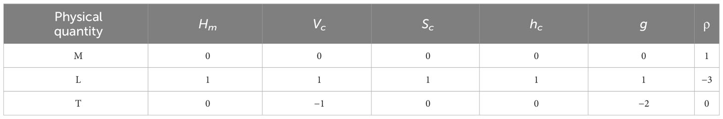
Table 3 Quantitative power exponents of the variables in the maximum wave height problem during the propagation of a ship-generated wave.

According to π theorem, S_c and h_c represent two independent variables that choose one as the reference physical quantity. In addition, V_c, g, and ρ should choose two as the physical reference quantity. In the present work, V_c, g, and ρ are selected as the reference physical quantity. For the sake of the classification of the abovementioned magnitudes sorted, as presented in Table 4.

TABLE 4

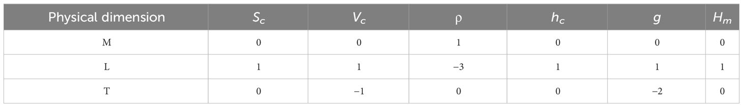
Table 4 Quantitative power exponents of the variables in the maximum wave height problem during the propagation of a ship-generated wave.

Thus, the expressions of the basic measure factors are derived from the reference measure in the following form:

$\begin{array}{ll}\{\begin{array}{l}\text{M}=[\mathit{\text{ρ}}]{[S_c]}^3\hfill \\ L=[S_c]\hfill \\ T=[S_c]{[V_c]}^{-1}\hfill \end{array}& \text{(1-5)}\end{array}$

After applying the transformation in Equation (1-5) to Table 4, one can arrive at Table 5.

TABLE 5

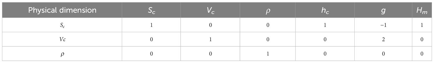
Table 5 Power exponent after line transformation of the variables used in the maximum wave height problem during propagation of a ship-generated wave.

Then, three dimensionless factors are given as follows:

$\begin{array}{ll}\{\begin{array}{l}{\prod }_1=\frac{h_c}{S_c}\\ {\prod }_2=\frac{g{S}_c}{V_c{}^2}\\ \prod =\frac{H_m}{S_c}\end{array}& \text{(1-6)}\end{array}$

As a result, the above-displayed problem can be described as follows:

$\begin{array}{ll}\frac{H_m}{S_c}=f(\frac{h_c}{S_c},\frac{g{S}_c}{V_c{}^2})& \text{(1-7)}\end{array}$

In Equation (1-6), dimensionless Π₁ represents the ratio of the water depth of the channel and the distance from the point to the ship’s side, which does not have practical significance. Therefore, the product of dimensionless factors Π₁ and Π₂ can be employed to express the relationship between the water depth and the Froude number. By this virtue, the correction and simplification of dimensionless Π₁ take the following form:

$\begin{array}{ll}{\prod }_1=\frac{H_c}{S_c}·\frac{g{S}_c}{V_c^2}=\frac{g{h}_c}{V_c^2}=\frac{1}{F{r}_h^2}& \text{(1-8)}\end{array}$

Therefore, Equation (1-7) can be transformed to give

$\begin{array}{ll}\frac{H_m}{S_c}=f(\frac{1}{F{r}_h^2},\frac{g{S}_c}{V_c{}^2})& \text{(1-9)}\end{array}$

Considering that the water depth of the AA number is a dimensionless factor when the ship moves in a restricted channel, Equation (1-9) can be reduced as follows:

$\begin{array}{ll}\frac{H_m}{S_c}=\frac{1}{F{r}_h^2}f(\frac{g{S}_c}{V_c{}^2})& \text{(1-10)}\end{array}$

2.3 Basic principles of PSOA

The PSOA is an evolutionary computational technique, which is essentially derived from the study of bird predation behavior (Kennedy and Eberhart, 1995). It is mainly constructed based on the sharing of information by individual particles in the swarm. Thus, the direction of the evolutionary process of particle motion is influenced from disorder to order in the problem-solving space, so that the particles obtain the optimal solution or reach the most favorable position. Suppose N particles are forming a group in the search space consisting of a D-dimensional target, where the i-th particle can be represented as a D-dimensional vector in the following form:

$\begin{array}{ll}{X}_i=(x_{i1},x_{i2},···x_{iD}),i=1,2,···,N& \text{(2-1)}\end{array}$

The optimized velocity of the i-th particle is a D-dimensional vector, denoted by:

$\begin{array}{ll}{V}_i=(v_{i1},v_{i2},···v_{iD}),i=1,2,···,N& \text{(2-2)}\end{array}$

When the particle continues to be optimized, then the optimized D-dimensional vector becomes.

$\begin{array}{ll}{v}_{ij}(t+1)=w{v}_{ij}(t)+c_1{r}_1(t)[p_{ij}(t)-x_{ij}(t)]+c_2{r}_2(t)[p_{gj}(t)-x_{ij}(t)]& \text{(2-3)}\end{array}$

$\begin{array}{ll}{x}_{ij}(t+1)=x_{ij}(t)+v_{ij}(t+1)& \text{(2-4)}\end{array}$

where $v_{ij}(t)$ denotes the t-generation initial velocity, $w$ stands for the inertia weight, $c_1{r}_1(t)[p_{ij}(t)-x_{ij}(t)]$ signifies the individual step forward to the global optimal solution, $[p_{ij}(t)-x_{ij}(t)]$ represents the step forward to the individual optimal solution position, and $c_1$ is the individual learning coefficient, $c_2{r}_2(t)[p_{gj}(t)-x_{ij}(t)]$denotes the step forward to the global optimal solution of the population, $[p_{gj}(t)-x_{ij}(t)]$ represents the optimal position of the population, $c_2$ is the population learning coefficient, $x_{ij}(t+1)$ signifies the coordinate position of the t+1 generation, determined by $x_{ij}(t)$ at t generation position and the t+1 generation speed ($v_{ij}(t+1)$). Therefore, as illustrated in Figure 4, the trajectory of the optimization algorithm can be interpreted as follows. Assuming that the current particle position is a particle, denoted by C, the individual optimization direction is B, and the global optimization direction is A. By applying individual and global optimizations, the particle moves to C and finally reaches the global optimal position A through continuous iterations.

FIGURE 4

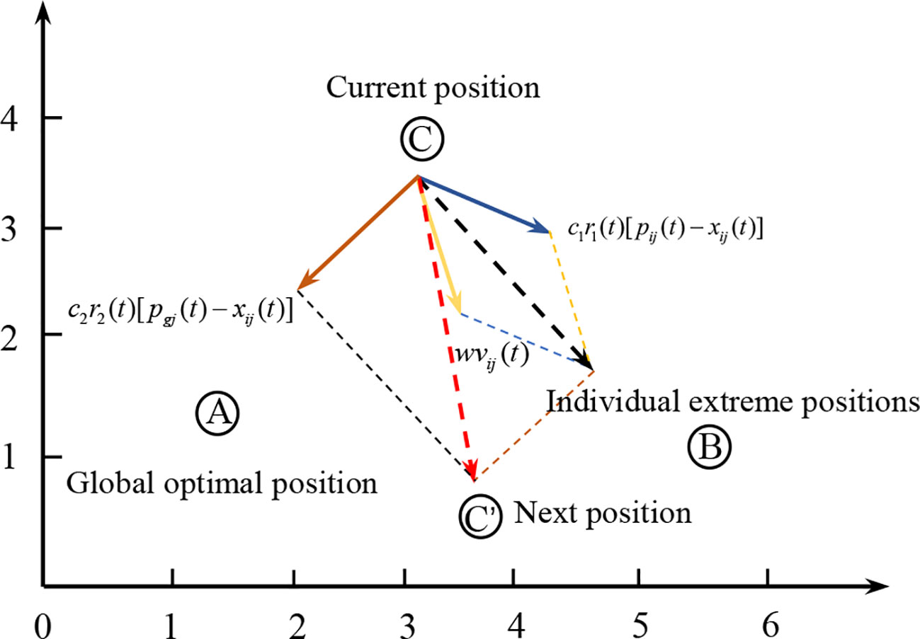
Figure 4 PSOA path diagram.

3 Results and discussion

For channels with shallow water depth and narrow channels, the ship-generated waves move along the side of the ship toward the shore and cause scouring of the riverbank. The degree of erosion of the riverbank by waves depends on the maximum wave height of the waves, which is presented in Figure 5.

FIGURE 5

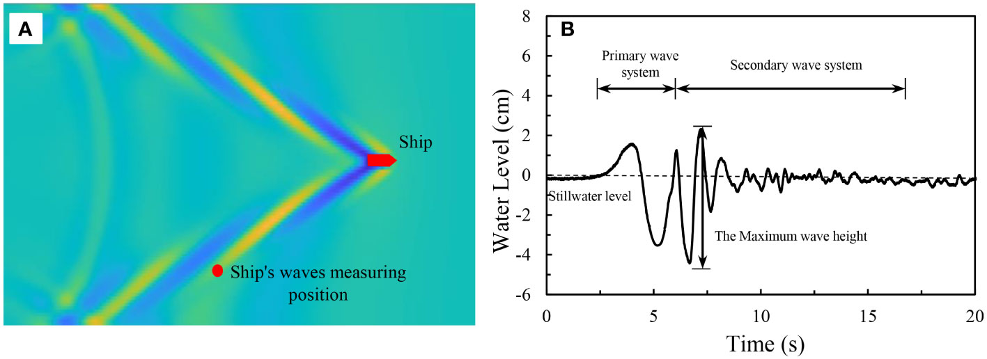
Figure 5 (A) A sketch of the typical ship wave and measuring position. (B) The fluctuation processes and maximum wave heights of the ship’s waves.

3.1 Distribution of maximum wave height with cross-section

The maximum wave height generated by the ship (H_m) under different navigation conditions is different, but the propagation process with the sectional distribution has a similar pattern, as illustrated in Figures 6A–C. Figure 6A shows the change of wave height in sections W1–W7 at different ship speeds in the case of h_c = 0.19 m. In general, the maximum wave height in the channel (H_m) tends to decay with the increase of S_c, while the variation of the maximum wave height (H_m) sectional distribution at the side slope of the channel is mostly related to the ship speed and then exhibits a descending trend. When the ship speed increases to 1.25 m/s to 1.42 m/s, the ship speed is mainly placed in the cross-critical region (i.e., 0.85 < Fr_h < 1.15). Under such circumferences, the overall wave height of the channel section exhibits an increasing trend, and the maximum wave height in this area demonstrates a slight increase or decrease trend as the ship speed continues to increase. The main reason behind this fact is that, when the ship line wave propagates in the navigation channel, it is mainly influenced by the low friction and the viscous force of the water. When the water depth sharply reduces after entering the slope and the reflection effect of the beach slope, the wave height of the ship line wave grows more than the reduction of the wave height of the bed friction, so it exhibits a slightly increasing trend. Because the water depth of the channel slope gradually becomes shallower, the bed friction increases; when the bed friction height decreases more than the wave height due to decreasing water depth, the maximum wave height begins to show a decreasing trend. Therefore, the attenuation of the maximum wave height (H_m) in the bank slope is less than that in the channel. When the shipping speed increases to 1.68 m/s, it will arrive at the supercritical region (Fr_h > 1.15), and the maximum overall wave height of the channel in this region exhibits a decreasing trend. Such an issue is mainly ascribed to the fact that the water depth and river width of the restricted channel is small, and the ship would have a great influence on the water surface when sailing at high speed. As the shipping speed increases, the wave height of the shipping line also increases; when the speed of the ship reaches a certain level, the water level drops too high, leading to the maximum wave height of the ship line wave to breaking. This causes a reduction of the wave height, then the maximum wave height increases in the slope area of the channel with the increase of S_c.

FIGURE 6

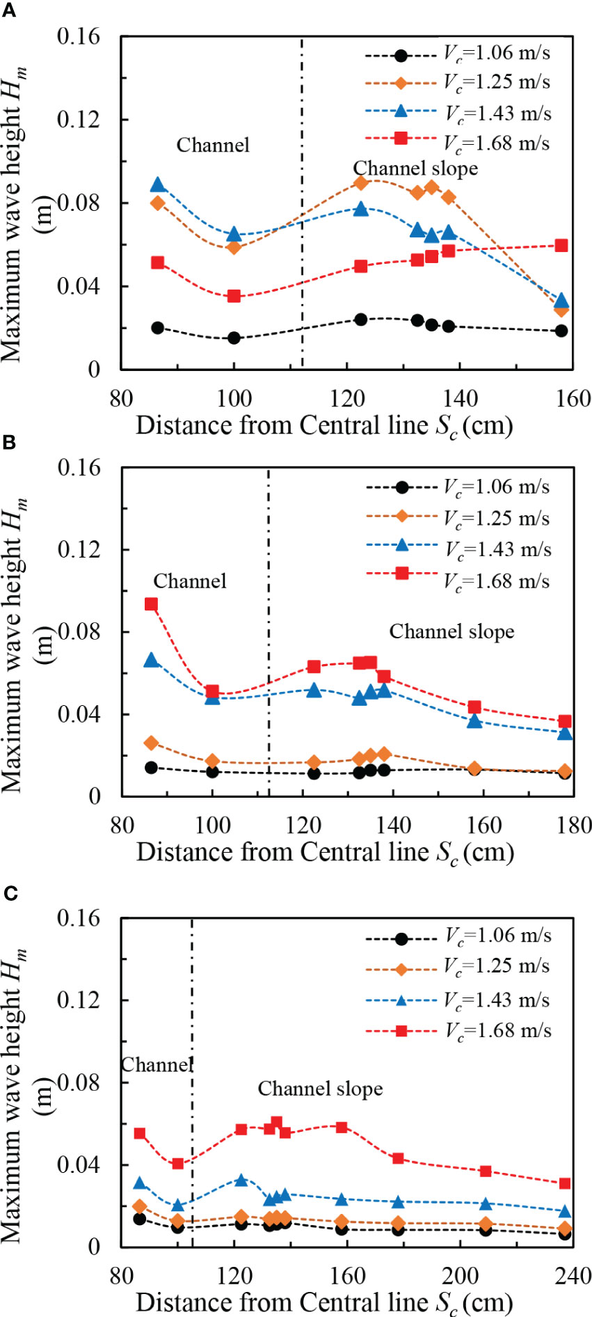
Figure 6 Maximum wave height distribution in channel sections in the presence of various navigation speeds: (A) h_c = 0.19 m, (B) h_c = 0.29 m, and (C) h_c = 0.39 m.

Figure 6B illustrates the wave height changes of measurement points W1–W8 at different boat speeds in the case of h_c = 0.29 m. Generally, the height of the ship traveling wave shows a positive correlation with the ship speed due to the increase of water depth in the channel. As is seen for Fr_h ≤ 0.84 (when the ship speed V_c ≤ 1.42 m/s), the maximum wave height is not affected by the water depth. The overall variation pattern of the maximum wave height below this water depth indicates that the wave height is smaller in the navigation channel during the transition from the navigation channel in the shore slope. When the shipping speed grows to 1.68 m, at this time, Fr_h = 0.86, and its section change law is similar to the cross-critical region for h_c = 0.19 m. Figure 6C illustrates that, in the case of h_c = 0.39 m, the variation of wave height at W1–W10 measurement points with ship speed (V_c) of 1.06 m/s to 1.42 m/s is the same as the distribution of maximum wave height at the section in the case of h_c = 0.29 m, and the increase of maximum wave height of ship moving wave raises with the increase of ship speed. In summary, the maximum wave height of the ship propagating waves in the channel and on the beach, slope is not compatible with the variation pattern of S_c. The maximum wave height of the ship propagating waves on the beach slope exhibits a decreasing trend, while the variation pattern of H_m on the beach slope is related to the water depth Froude number.

3.2 Variation of the maximum wave height with ship speed

In order to investigate the effect of ship speed and water depth on the maximum wave height of ship traveling waves at various measurement points in the channel, the measurement points at three water depths are not consistent; therefore, the measurement data of three different water depths at measurement points W1–W6 are methodically examined, as illustrated in Figures 7A–F. The relationships between the maximum wave heights of the ship traveling waves and the ship speeds at the measurement points W1–W6 in the channel have similarities. The ship speed (V_c) and the maximum wave height (H_m) exhibit three different relationships, and the relationship curve is mainly determined by the water depth. When the water depth of the channel is set as h_c = 0.19 m, the maximum wave height shows an increasing and then decreasing trend with the speed of the ship. When the water depth of the restricted water is small, the resistance of the ship is larger when the ship is sailing at a lower speed. Furthermore, the maximum wave height of the ship is larger than that in deeper water conditions, and the increase of the shipping speed exhibits a gradual ascending trend. When the speed reaches a certain value, the maximum wave height takes its peak point. When the speed of the ship gradually increases, the maximum wave height of the ship line wave also gradually increases, and the period is gradually decreasing. The peak of the wave becomes sharper as the shipping speed increases. Furthermore, the ratio of the maximum height of the ship line wave and the water depth (H_m/h_c) becomes greater than a certain value, the wave has a tendency to attenuate or even break, and H_m commences to become smaller. When the water depth of the channel raises to h_c = 0.29 m and h_c = 0.39 m and the shipping speed grows from 1.03 m/s to 1.68 m/s, the effect of ship speed on the maximum wave height exhibits a positive correlation trend, and the shallower the water depth, the higher the wave height with the shipping speed. However, the increase in wave height is greater with the ship speed.

FIGURE 7

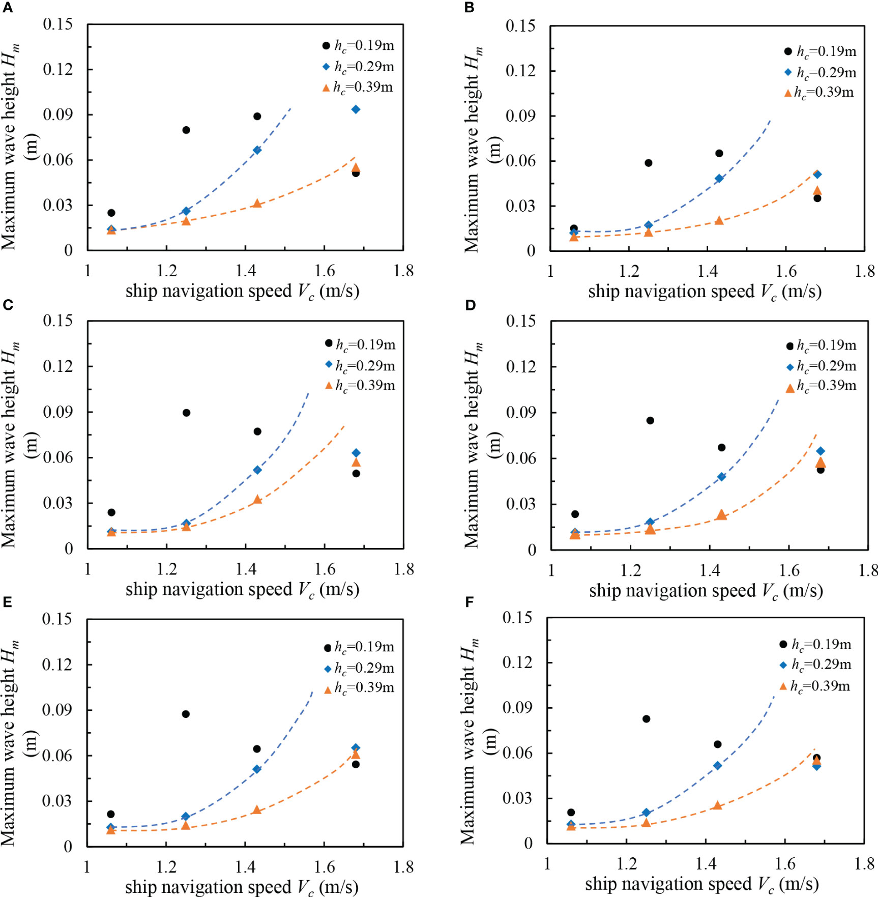
Figure 7 Effect of speed on the maximum wave height of a ship-generated waves at different water depths for various measuring points: (A) W1, (B) W2, (C) W3, (D) W4, (E) W5, and (F) W6.

In summary, the maximum wave height is determined by the shipping speed (V_c) and the water depth (h_c). Based on this important factor that the propagation pattern of ship waves in restricted waters is determined by the Froud number of the water depth, the relationship among the water depth, the Froud number (Fr_h), and the maximum wave height of the ship waves can be determined by dimensionless quantification of the shipping speed from W1 to W6 under various working conditions, as demonstrated in Figure 8. In the case of Fr_h< 0.84, the corresponding ship speed is placed in the sub-critical speed region and the maximum wave height in this region grows as the ship speed increases (Dam et al., 2008), demonstrating a positive trend. For the case of 0.84< Fr_h< 1.15, the ship speed is placed in the critical speed region, and the wave height exhibits an increasing and then decreasing speed in terms of the Froude number and touches its peak at 0.92 ≤ Fr_h ≤ 1.05. In the case of Fr_h > 1.15, the shipping speed is placed in the supercritical speed area, the maximum wave height of the ship-generated wave and water depth Froude number (Fr_h) raise and lessen sharply, are inversely proportional to the trend, and its law and subcritical region change law are almost opposite. When the ship travels in the trough, the ship travels with a gradually decreasing wave, and the water depth Froude number associated with the maximum wave height changes from Fr_h = 0.99 to Fr_h = 1.05. The maximum wave height increases suddenly after entering the channel side slope, and the water depth Froude number pertinent to the maximum wave height at its maximum value varies from Fr_h = 1.05 to Fr_h = 0.92. Hence, the wave height decay during the propagation of the ship traffic wave will lead to a larger maximum wave height Froude number at this measurement point, whereas the increase of the ship traffic wave leads to a smaller maximum wave height water depth Froude number.

FIGURE 8

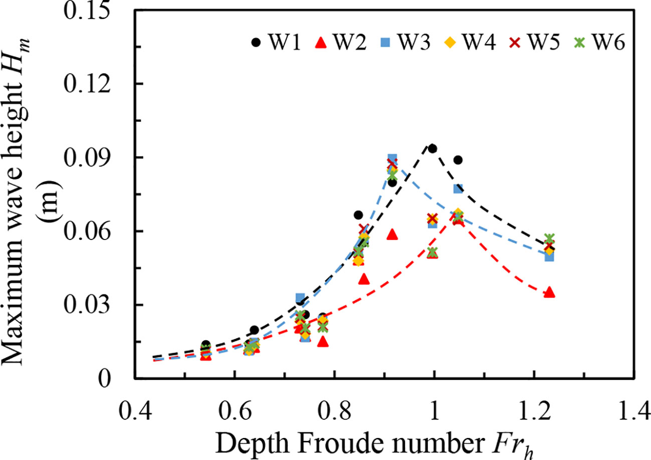
Figure 8 Relationship between the water depth Froude number (Fr_h) and the maximum wave height.

3.3 Prediction of maximum wave height equations for restricted channel slopes

According to the aforementioned cross-section of the ship’s wave along the channel in confined waters, it can be seen that the maximum wave height of the ship wave at the measurement points of the channel varies irregularly in both the cross-critical and supercritical velocity regions, whereas a specific regular distribution is detectable in the subcritical speed region (Fr_h< 0.84). This enables us to carefully analyze the maximum measured wave height on the beach slope at the measuring point W3–W10 in restricted waters under different working conditions. The dimensionless derivation in Equation (1-10) of the proposed approach shows that the maximum wave height (H_m) of the ship’s wave at a certain location in the channel can be stated as a function of the ship’s navigation speed (V_c), the transverse distance between the center of the channel and measurement point (S_c), and water depth Froude number (Fr_h). This relation can be obtained by the equation conversion in the following form:

$\begin{array}{ll}\frac{H_{m}F{r}_h^2}{S_c}=f(\frac{g{S}_c}{V_c{}^2})& \text{(1-11)}\end{array}$

Based on the abovementioned ship navigation conditions at various water depths and the results of the wave height meter, the relevant measurement data are dimensionless and the horizontal and vertical coordinates are set as $\frac{g{S}_c}{V_c{}^2}$ and $\frac{H_{m}F{r}_h^2}{S_c}$, respectively. The relationship between $\frac{g{S}_c}{V_c{}^2}$ and $\frac{H_{m}F{r}_h^2}{S_c}$ can be derived for channel water depths of h_c = 0.19 m, 0.29 m, and 0.39 m. As presented in Figure 9, Figure 9A illustrates the distribution of the ship speed at each measurement point in the subcritical region at h_c = 0.19 m, and the measured values of W3–W7 at V_c = 1.03 m/s are dimensionless. Figure 9B exhibits the distribution of the shipping speed in the subcritical region for h_c = 0.29 m, and the measured values of W3–W8 at V_c = 1.03 m/s, 1.21 m/s, and 1.43 m/s are all dimensionless. Figure 9C illustrates the distribution of ship speed in the sub-critical region at h_c = 0.39 m, and the measured values from W3–W8 at V_c = 1.03 m/s, 1.21 m/s, and 1.43 m/s are dimensionless. From the non-linear regression analysis, it can be obtained that $\frac{g{S}_c}{V_c{}^2}$ and $\frac{H_{m}F{r}_h^2}{S_c}$ in Figures 9A–C are distributed in a power exponential form, and their correlation coefficients R² are all greater than 0.9; therefore, this objective function can be written as:

FIGURE 9

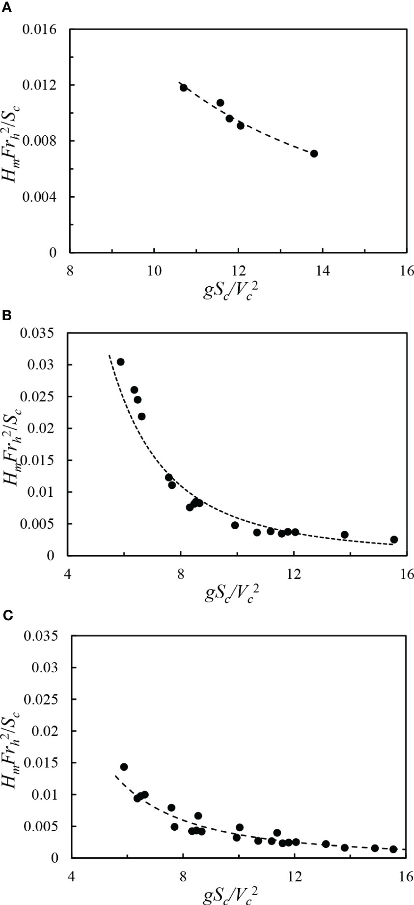
Figure 9 Correlation between $\frac{g{S}_c}{V_c{}^2}$ and $\frac{H_{m}F{r}_h^2}{S_c}$ for various water depths: (A) h_c = 0.19 m, (B) h_c = 0.29 m, (C) h_c = 0.39 m.

$\begin{array}{ll}\frac{H_{m}F{r}_h^2}{S_c}=k_1{(\frac{g{S}_c}{V_c{}^2})}^{k_2}& \text{(1-12)}\end{array}$

In summary, first of all, according to the basic principles of least squares, we should construct the residual sum of squares of the objective function. To this end, take each pair’s values of k₁ and k₂ until the smallest value of the function is obtained, and then the corresponding values of k₁ and k₂ are then considered. When a ship is traveling in a given water depth, the predicted equation for the maximum wave height of the ship’s travel wave is given by $H_m=k_1\frac{S_c}{F{r}_h^2}{(\frac{g{S}_c}{V_c{}^2})}^{k_2}$. The ensemble of the measured wave heights at each measurement points of various ship speeds in the channel section at that water depth can be regarded as the ensemble of Y. Subsequently, the ensemble of the maximum wave heights of the measured ship’s travel waves can be provided by $Y_{}=(Y_1,Y_2,···Y_i)$. According to the prediction equation for the maximum wave height of a ship traveling wave, the calculated value of the maximum wave height of a ship traveling wave can be viewed as the ensemble of multiple X, namely, $X=f(S_{ci},F{r}_{hi},V_{ci}|k_1,k_2)$, where X is the relevant calculated parameter corresponding to the measured wave height, and k₁ and k₂ are the instantaneous coefficients. Then, the target residual sum-of-squares function, $F{(H_m)}_{SSE}$, can be stated by the following:

$\begin{array}{ll}{F}_{}{(H_m)}_{SSE}={{\displaystyle \sum _{i=1}^{i=N}[Y_i-f(S_{ci},F{r}_{hi},V_{ci}|k_1,k_2)]}}^2& \text{(2-5)}\end{array}$

Based on the PSOA, the residual sum-of-squares function can be evaluated iteratively for the maximum point of the wave height measurement. For this purpose, when the value reaches a minimum, at this point, the values of k₁ and k₂ represent instantaneous coefficients. The upper and lower limits of k₁ and k₂ parameters can be set as follows: 0 ≤ k₁ ≤ 6, −5 ≤ k₂ ≤ 5, where c₁ and c₂ are considered acceleration constants of value 2, and the minimum value of the residual sum of squares function can be found through iterative calculation. The measured values for these conditions and the calculated fit are shown in Figure 10. At h_c = 0.19 m, the measured maximum wave height (H_m) of the ship’s traveling wave and the fit based on the PSA essentially match for k_{1 =} 1.52 and k₂ = −2.04. When the water depth (h_c) increases to 0.29 m and the shipping speed is as small as V_c = 1.03 m/s, the measured value is the same as the fitted value. As the ship speed raises (V_c = 1.25 m/s), the fitted value is larger than the actual maximum wave height measured. When the shipping speed increases to 1.43 m/s, the increase of the fitted value is smaller than the measured value. When the PSA is employed to perform the optimization, it should consider three at the same time. The maximum wave height generated by various speeds has an impact on it, and the increase in maximum wave height for the ship speed increase from 1.03 m/s to 1.25 m/s is much less than that for the increase of ship speed from 1.25 m/s to 1.43 m/s. The fitted curve should be appropriately integrated with different increase values to show the law, in the case of k_{1 =} 5.30, k₂ = −2.94. As the water depth increases to 0.39 m, the corresponding values are in general agreement with the measured values, and the increase in maximum wave height and ship speed of the ship traveling wave are also consistent with k_{1 =} 1.08 and k₂ = −2.50.

FIGURE 10

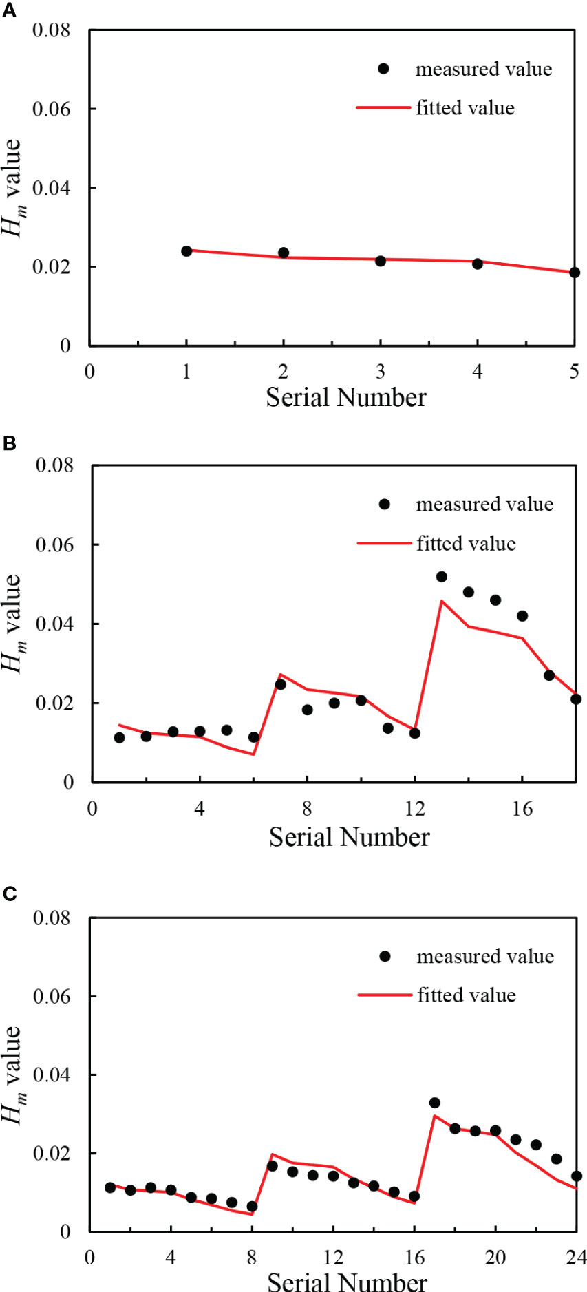
Figure 10 Comparison between the fitted values and the measured values based on the PSA used for solving the fitted relations: (A) Comparison of the measured and fitted values of the bank slope at V_c = 1.03 m/s for a water depth of h_c = 0.19 m in channel. (B) Comparison of the measured and fitted values of the bank slope measurement points at V_c = 1.03 m/s, V_c = 1.25m/s, and V_c = 1.43 m/s for a channel water depth of h_c = 0.29 m. (C) Comparison of the measured and fitted values of the bank slope at V_c = 1.03 m/s, V_c = 1.25 m/s, and V_c = 1.43 m/s for a water depth of h_c =0.39 m in the navigation channel.

To compare the accuracy of the PSA to solve the equation model and determine the goodness of fit, the most extensively implemented methodologies are the traditional least squares method and the Fmincon function. In this regard, the sum of squares due to error (SSE), the sum of squares (SST), and the coefficient of determination (R²) of the goodness of fit of the model are evaluated for the maximum wave height prediction equation model, where $R^2=1-\frac{SSE}{SST}$. The values for each of the different water depth conditions are provided in Table 6. The prediction equations for the maximum wave height of the ship traveling wave associated with three different solution methods restrict the prediction model of the maximum ship traveling wave equation in the beach slope; as a general rule, the lower the residual sum of squares, the higher the prediction accuracy. In general, the PSA has the best overall effect, and the least squares method and the Fmincon function solution method are the same. Their decision coefficients are slightly lower than those of the PSA, but the equation model behaves better (R² ≥ 0.85). The least squares and Fmincon function solution approaches have many iterations and tend to fall into local optimal solutions, while the PSA avoids falling into local optimal solutions by combining individual extreme values and overall optimal solutions. Briefly, the PSA solves the prediction equation for the maximum wave height in shallow water for $H_m=k_1\frac{S_c}{F{r}_h^2}{(\frac{g{S}_c}{V_c{}^2})}^{k_2}$ with a fit goodness R² ≥ 0.88, and the prediction results are close to the measured values. The values of k₁ and k₂ for various water depth conditions are presented in Figure 11.

TABLE 6

Table 6 Sum of squares due to error (SSE), the sum of squared total (SST), and coefficient of determination (R²) of the goodness of fit of the model for the fitted equations for various water depth conditions.

FIGURE 11

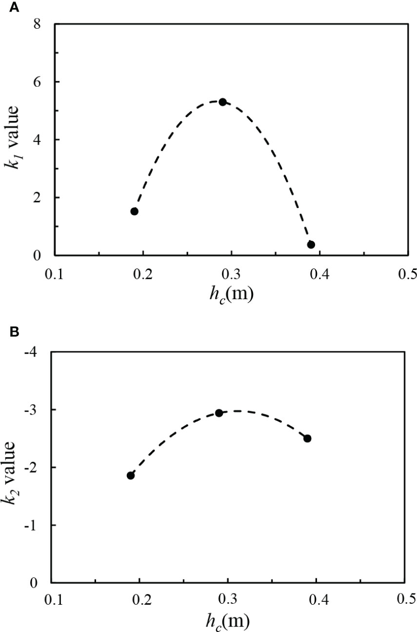
Figure 11 Values of k₁ and k₂ for various water depths: (A) k₁ value and (B) k₂ value.

4 Conclusion

In the current investigation, the actual channel section is methodically simulated by a large indoor flume, and a ship self-propelled experiment is appropriately carried out. The wave height meter is arranged according to the channel section to analyze the monitoring data of the ship-generated waves and examine the relationship among the maximum wave height, the shipping speed, and water depth at the measurement points. The type of prediction function of the maximum wave height in a trapezoidal channel and the residual sum of squares function of the prediction equation and the measured values are constructed using dimensional analysis. Subsequently, the minimum value of the residual sum of squares function is appropriately solved by a PSOA to arrive at the optimal coefficients k₁ and k₂ of the prediction function. As a result, the prediction equation of the maximum wave height (H_m) is obtained for the ship-generated waves adapted to the slope of the channel within restricted waters. The main obtained results are summarized as follows:

(1) A large flume is utilized to simulate a trapezoidal section of restricted waters to examine the distribution pattern of the maximum wave height in the section at different ship speeds and depths. It is observed that the wave height in the flume and the slope when the wave is propagated from the center of the channel to the slope of the trapezoidal section.

(2) The maximum wave height is determined by both the water depth and the speed of the ship, so its variation law can also be described by the water depth Froude number. As the bathymetric Froude number (Fr_h) increases, the maximum wave height increases and reaches a maximum value as the value of Fr_h raises to around 1.

(3) The function relationship: $\frac{H_{m}F{r}_h^2}{S_c}=f(\frac{g{S}_c}{V_c{}^2})$ is achieved by appropriate dimensional analysis of the factors influencing the maximum wave height of ship-generated waves in the trapezoidal section channel, and the function type $\frac{H_{m}F{r}_h^2}{S_c}=k_1{(\frac{g{S}_c}{V_c{}^2})}^{k_2}$ is then determined. According to the PSA used in the subcritical velocity region (Fr_h< 0.84), for various water depths, wave heights, shore slopes, and the sum of squares minimum value, the function was solved for the appropriate values of k₁ and k₂. A relationship between the water depth of the channel and k₁ and k₂ values is constructed and, finally, the prediction equation of the maximum wave height for the channel shore slope region is suitably proposed.

Data availability statement

The raw data supporting the conclusions of this article will be made available by the authors, without undue reservation.

Author contributions

WH: Experimentalize, Methodology, Formal analysis, Writing - original draft. SL: Validation, Writing - review and editing. YL: Funding acquisition. RZ: Experimental assistant, Investigation. HW: Investigation. All authors contributed to the article and approved the submitted version.

Conflict of interest

The authors declare that the research was conducted in the absence of any commercial or financial relationships that could be construed as a potential conflict of interest.

Publisher’s note

All claims expressed in this article are solely those of the authors and do not necessarily represent those of their affiliated organizations, or those of the publisher, the editors and the reviewers. Any product that may be evaluated in this article, or claim that may be made by its manufacturer, is not guaranteed or endorsed by the publisher.

Abbreviations

C_a, channel cross-sectional coefficient; w, water surface width of the channel; L_v, length of the ship; D, draught of the ship; S_c, distance from the ship’s course to the measurement point; A’’, volume factor; B, ship’s width; H_m, maximum wave height of the ship-generated wave; h_c, water depth of the channel; V_c, navigation speed of the ship; S_c, horizontal distance from wave gauge; h_p, calculation point water depth; g, acceleration of gravity; ρ, density of water; $w$, inertia weight; $c_1$, individual learning coefficient; $c_2$, population learning coefficient; k₁ and k₂, constant value; R², coefficient of determination.

References

Balanin V., Bykov L. (1965). Selection of leading dimensions of navigation channel sections and modern methods of bank protection. Proceedings of the 21st International Navigation Congress. (Stockholm: PIANC).

Google Scholar

Bhowmik N. G. (1975). Boat-generated waves in lakes. J. Hydraulics. Division. 101, 1465–1468. doi: 10.1061/JYCEAJ.0004439

CrossRef Full Text | Google Scholar

Bhowmik N. G., Demissie M., Guo C.-Y. (1982). Waves generated by river traffic and wind on the Illinois and Mississippi Rivers. ISWS. Contract. Rep. CR. 293 RR-117. Available at: http://hdl.handle.net/2142/72711.

Google Scholar

Bhowmik N. G., Soong T. W., Reichelt W. F., Seddik N. M. L. (1991). Waves generated by recreational traffic on the Upper Mississippi river system. ISWS. RR-117. Available at: https://www.ideals.illinois.edu/items/77055.

Google Scholar

Bilkovic D. M., Mitchell M. M., Davis J., Herman J., Andrews E., King A., et al. (2019). Defining boat wake impacts on shoreline stability toward management and policy solutions. Ocean. Coast. Manage. 182, 104945. doi: 10.1016/j.ocecoaman.2019.104945

CrossRef Full Text | Google Scholar

Buckingham E. (1914). On physically similar systems; illustrations of the use of dimensional equations. Phys. Rev. 4, 345. doi: 10.1103/PhysRev.4.345

CrossRef Full Text | Google Scholar

Cameron H., Bauer B. (2014). River bank erosion processes along the lower Shuswap river. Final Project Report submitted to Regional District of North Okanagan (University of British Columbia Okanagan).

Google Scholar

Dam K. T., Tanimoto K., Fatimah E. (2008). Investigation of ship waves in a narrow channel. J. Mar. Sci. Technol. 13, 223–230. doi: 10.1007/s00773-008-0005-6

CrossRef Full Text | Google Scholar

Du P., Ouahsine A., Sergent P., Hu H. (2020). Resistance and wave characterizations of inland vessels in the fully-confined waterway. Ocean. Eng. 210, 107580. doi: 10.1016/j.oceaneng.2020.107580

CrossRef Full Text | Google Scholar

Fleit G., Hauer C., Baranya S. (2021). A numerical modeling-based predictive methodology for the assessment of the impacts of ship waves on YOY fish. River. Res. Appl. 37, 373–386. doi: 10.1002/rra.3764

CrossRef Full Text | Google Scholar

Havelock T. H. (1922). The effect of shallow water on wave resistance. Proc. R. Soc. London. Ser. A. Containing. Papers. Math. Phys. Character. 100, 499–505. doi: 10.1098/rspa.1922.0013

CrossRef Full Text | Google Scholar

Hofmann H., Lorke A., Peeters F. (2008). The relative importance of wind and ship waves in the littoral zone of a large lake. Limnol. Oceanogr. 53, 368–380. doi: 10.4319/lo.2008.53.1.0368

CrossRef Full Text | Google Scholar

Jägerbrand A. K., Brutemark A., Sveden J. B., Gren M. (2019). A review on the environmental impacts of shipping on aquatic and nearshore ecosystems. Sci. Total. Environ. 695, 133637. doi: 10.1016/j.scitotenv.2019.133637

PubMed Abstract | CrossRef Full Text | Google Scholar

Kennedy J., Eberhart R. (1995). Particle swarm optimization. Proceedings of ICNN'95-international conference on neural networks. IEEE. 1942–1948.

Google Scholar

Kriebel D. L., Seelig W. N. (2005). An empirical model for ship-generated waves. Proceedings of the 5th international symposium on ocean wave measurement and analysis.

Google Scholar

Kurdistani S. M., Tomasicchio G. R., D'alessandro F., Hassanabadi L. (2019). River bank protection from ship-induced waves and river flow. Water Sci. Eng. 12, 129–135. doi: 10.1016/j.wse.2019.05.002

CrossRef Full Text | Google Scholar

Li Y., Ellingsen S. Å. (2016). Ship waves on uniform shear current at finite depth: wave resistance and critical velocity. J. Fluid. Mechanics. 791, 539–567. doi: 10.1017/jfm.2016.20

CrossRef Full Text | Google Scholar

Mao L., Chen Y. (2020). Investigation of ship-induced hydrodynamics and sediment suspension in a heavy shipping traffic waterway. J. Mar. Sci. Eng. 8, 424. doi: 10.3390/jmse8060424

CrossRef Full Text | Google Scholar

Maynord S. T. (2005). Wave height from planing and semi-planing small boats. River. Res. Appl. 21, 1–17. doi: 10.1002/rra.803

CrossRef Full Text | Google Scholar

Nanson G. C., Von Krusenstierna A., Bryant E. A., Renilson M. R. (1994). Experimental measurements of river-bank erosion caused by boat-generated waves on the Gordon River, Tasmania. Regulated. Rivers.: Res. Manage. 9, 1–14. doi: 10.1002/rrr.3450090102

CrossRef Full Text | Google Scholar

Noblesse F., He J., Zhu Y., Hong L., Zhang C., Zhu R., et al. (2014). Why can ship wakes appear narrower than Kelvin’s angle? Eur. J. Mechanics-B/Fluids. 46, 164–171. doi: 10.1016/j.euromechflu.2014.03.012

CrossRef Full Text | Google Scholar

Ozeren Y., Simon A., Altinakar M. (2016). “Boat-generated wave and turbidity measurements: connecticut river,” in World environmental and water resources congress 2016. 390–398.

Google Scholar

Paatero P., Tapper U. (1993). Analysis of different modes of factor analysis as least squares fit problems. Chemometrics. Intelligent. Lab. Syst. 18, 183–194. doi: 10.1016/0169-7439(93)80055-M

CrossRef Full Text | Google Scholar

Pianc (1987). Guidelines for the design and construction of flexible revetments incorporating geotextiles for inland waterways: report of working group 4 of the permanent technical committee I. PIANC.

Google Scholar

Rapaglia J., Zaggia L., Ricklefs K., Gelinas M., Bokuniewicz H. (2011). Characteristics of ships' depression waves and associated sediment resuspension in Venice Lagoon, Italy. J. Mar. Syst. 85, 45–56. doi: 10.1016/j.jmarsys.2010.11.005

CrossRef Full Text | Google Scholar

Safty H. E., Marsooli R. (2020). Ship wakes and their potential impacts on salt marshes in Jamaica bay, New York. J. Mar. Sci. Eng. 8, 325. doi: 10.3390/jmse8050325

CrossRef Full Text | Google Scholar

Scarpa G. M., Zaggia L., Manfè G., Lorenzetti G., Parnell K., Soomere T., et al. (2019). The effects of ship wakes in the Venice Lagoon and implications for the sustainability of shipping in coastal waters. Sci. Rep. 9, 1–14. doi: 10.1038/s41598-019-55238-z

PubMed Abstract | CrossRef Full Text | Google Scholar

Sorensen R. M. (1997). Prediction of vessel-generated waves with reference to vessels common to the upper Mississippi River system. ENV Report 4[J] US Army Corps of Engineers. Available at: https://trid.trb.org/view/584925.

Google Scholar

Stumbo S. (2001). An assessment of wake wash reduction of fast ferries at supercritical Froude numbers and at optimized trim. Proceedings of the technical conference of 6th china international boat show, Shanghai. China, April 2001.

Google Scholar

Suprayogi D. T., Bin Yaakob O., Ahmed Y. M., Hashim F. E., Prayetno E., Elbatran A. A., et al. (2022). Speed limit determination of fishing boats in confined water based on ship generated waves. Alexandria. Eng. J. 61, 3165–3174. doi: 10.1016/j.aej.2021.08.045

CrossRef Full Text | Google Scholar

Teatini P., Isotton G., Nardean S., Ferronato M., Mazzia A., Da Lio C., et al. (2017). Hydrogeological effects of dredging navigable canals through lagoon shallows. A case study in Venice. Hydrol. Earth System. Sci. 21, 5627–5646. doi: 10.5194/hess-21-5627-2017

CrossRef Full Text | Google Scholar

Uncles R., Stephens J., Harris C. (2014). Freshwater, tidal and wave influences on a small estuary. Estuarine. Coast. Shelf. Sci. 150, 252–261. doi: 10.1016/j.ecss.2014.05.035

CrossRef Full Text | Google Scholar

U.S. Army Corps of Engineers, H.D (1980). “Gallipolis locks and dam replacement, Ohio River, phase I - advanced engineering and design study,” in General Design Memorandum, Huntington, WV.

Google Scholar

Williams A., Rangel-Buitrago N., Pranzini E., Anfuso G. (2018). The management of coastal erosion. Ocean. Coast. Manage. 156, 4–20. doi: 10.1016/j.ocecoaman.2017.03.022

CrossRef Full Text | Google Scholar