Low-cost UAV monitoring: insights into seasonal volumetric changes of an oyster reef in the German Wadden Sea

1 Introduction

The climate crisis entails increasing ocean temperatures, rising sea levels and acidification which affect marine ecosystems, leading to ecological changes (IPCC, 2018). The ecological shift can partially transform ocean and coastal environments with irreversible degradation and risk of biodiversity losses (IPCC, 2022). Increasing local ocean temperatures may deteriorate but enhance living conditions (Doney et al., 2012) and promote species translocations. Benefiting from the rising water temperatures in the North Sea, the non-native Pacific oyster Magallana gigas (Thunberg (1793), formerly Crassostrea gigas) has invaded the East Frisian Wadden Sea through larvae drift, mainly from aquaculture plots in the Netherlands in the late 1990s (Wehrmann et al., 2000; Beukema and Dekker, 2005; Schmidt et al., 2008).

The Pacific oyster has transformed native blue mussel (Mytilus edulis, von Linné and Salvius (1758)) beds into three-dimensional (3D)-structural reef complexes with highly rough surfaces and replaced the blue mussel in its function as an ecosystem engineering species (Brandt et al., 2008; Markert et al., 2013; Bungenstock et al., 2021).

Prior to the bioinvasion, the blue mussel dominated the tidal flat sediment surface affecting biological and physical conditions such as the bottom roughness (Peine et al., 2005), the boundary layer and sedimentation processes (Gutiérrez et al., 2003; Norling and Kautsky, 2007; van der Zee et al., 2012). The blue mussels offer a suitable and often the only accessible hard substrate for the oyster larvae to settle on in the intertidal zone (Wehrmann et al., 2000; Brandt et al., 2008; Wrange et al., 2010). Oysters cement themselves to these hard surfaces and their adjacent conspecifics, building solid oyster-sediment matrices (Burkett et al., 2010; Tibabuzo Perdomo et al., 2018). These structures grow with each generation, and older individuals located deeper can be covered or buried by sedimentation and younger oyster generations. When individuals die, the shells remain and provide further substrate to settle (Diederich, 2005; de Paiva et al., 2018). Depending on the age of a reef, the internal reef structures differ locally in abundance, sediment coverage, shell growth and orientation, forming different patterns and roughness levels within the reef (Bungenstock et al., 2021; Hitzegrad et al., 2022).

The transformation from mussel beds to oyster reefs has caused an irreversible ecological shift in the benthic habitat (Schmidt, 2009; Folmer et al., 2014; Reise et al., 2017) and may change populations of benthic species. However, the reefs also offer a wide range of ecosystem services, such as filtering water, carbon sequestration, nursery habitats, biological biodiversity and regulation of nutrients (Morrison et al., 2014; Chand and Bollard, 2021b; Windle et al., 2022). Besides ecological changes, the complex 3D-reef structures, typically covering nowadays broad spatial areas, affect local hydro- and morphodynamics and vice versa in the German Wadden Sea (García-March et al., 2007; Markert et al., 2010; Folmer et al., 2014). Oyster reefs can mitigate flow and wave energy as living breakwaters (Scyphers et al., 2011; Bouma et al., 2014; Manis et al., 2015) and stabilise surrounding sediment (Piazza et al., 2005; de Paiva et al., 2018; Chowdhury et al., 2019). Considering future extreme sea levels (IPCC, 2021), the flow-attenuating features could be a part of future coastal protection measurements and extend far outside their reefs, affecting tidal flats and protecting the surrounding soft-sediment environment against erosion (Walles et al., 2015). Mitigating erosion and dissipating hydrodynamic energy are anticipated at the lee side that may promote vegetation growth (Sharma et al., 2016a; Sharma et al., 2016b) besides sediment accumulation (de Paiva et al., 2018).

Oyster reefs comprise densely packed and well-cemented valves; they thus resist remarkably well to forces exerted by waves, tidal currents, and ice drift. This feature is much more pronounced than for blue mussel beds (Bungenstock et al., 2021), resulting in higher survival chances for oysters, once initial reef settlements have been established. However, the habitat must meet specific environmental conditions for the Pacific oyster, including several biological and physical factors. There is only a little understanding of the maximum elevation reached by Pacific oyster reefs at tidal coasts, as their vertical growth depends on the water level. Thus, a possible correlation between reef elevation and the water level should be investigated.

While the Pacific oyster has spread out for more than two decades along the German west coast since its invasion from the Netherlands (Wehrmann et al., 2000), the global oyster population has suffered losses of about 85% worldwide (Beck et al., 2011) due to diseases, ocean heating and anthropogenic activities such as overfishing and pollution (Hogan and Reidenbach, 2022; Windle et al., 2022). Across the US Atlantic coastline, remote sensing has been employed to evaluate the American oyster’s (Crassostrea virginica, Gmelin (1791)) restoration attempts to enhance ecosystem services (Schulte et al., 2009; Grabowski et al., 2012; Hogan and Reidenbach, 2022). In contrast, previous studies of the settlement and exponential spread of the Pacific oyster in the North Sea have raised apprehension regarding the possible impact on the native community and surrounding tidal flats (Nehls and Büttger, 2007; Markert et al., 2010; Büttger et al., 2011).

However, recent studies have indicated enhancements such as increased biodiversity (Hollander et al., 2015; Zwerschke et al., 2020), coastal protection (Fivash et al., 2021; Hansen et al., 2023) and providing a habitat for various species through oyster reefs compared to blue mussel beds (Folmer et al., 2017).

In that context, it is paramount to access suitable methods and instrumentation that allow a more extensive spatial coverage and provide accuracies as temporal growth magnitudes across species-related cycles are in the order of <10 cm. In the past, oyster reefs have been surveyed using measurement methods, such as terrestrial laser scanning (TLS) (Fodrie et al., 2014; Rodriguez et al., 2014; Ridge et al., 2017a), airborne (Grizzle et al., 2002; Herlyn, 2005) and satellite surveys (Dehouck et al., 2013; Gade et al., 2014; Winter et al., 2016). The time-consuming TLS can yield high-resolution point clouds of reef structures, but more efficient methods cover broader areas. Using aerial photographs, Grizzle et al. (2002) distinguished dead oyster reefs from living oyster reefs by colour as a decisive parameter. As an active optical technique, airborne light detection and ranging (LiDAR) measures geometric structures with three-dimensional information and has become a standard tool for monitoring coastal zones (Adolph et al., 2017a). Optical airborne and satellite data are limited by daytime, tidal and weather conditions (Gade et al., 2014). To overcome these issues, electro-optical and high-resolution synthetic aperture radar (SAR) sensors of satellites were added to the optical data to measure the electromagnetic reflectance from the surface (Winter et al., 2016), independently from the tide, cloud coverage and poor light conditions (Nieuwhof et al., 2015). Choe et al. (2012), Nieuwhof et al. (2015) and Gade et al. (2014) could confirm an improved classification of mussel beds and other intertidal habitats in optical imagery when combined with TerraSAR-X images due to high surface roughness of mussel beds and oyster reefs, which increase the reflecting backscatter of the signal from the rough surfaces. Winter et al. (2016) tested a combination of remote sensing techniques for mapping and assessing intertidal flats in the German Wadden Sea, namely airborne LiDAR, electro-optical (RapidEye) and synthetic radar (SAR) sensors installed on satellites (Jung et al., 2015; Adolph et al., 2017a, Adolph et al., 2017b). Previous studies investigated mussel beds (including oysters), bedforms and other surface types via TerraSAR-X images but were limited in precisely determining the extension of bivalve beds (Müller et al., 2016).

Satellites and airborne surveys from higher altitudes cannot provide structural features such as roughness, slope and elevation on a high-resolution level to identify typical small-scale reef characteristics (Ridge et al., 2023). Therefore, adding structural features as training data on cm-scale may increase the classification success of oyster reefs.

In contrast to other monitoring techniques, unoccupied aerial vehicles (UAV) can increase the efficiency of monitoring oyster reefs due to a higher spatial resolution, similar accuracies to TLS and without physically influencing the field of investigation (Ridge et al., 2023). In the last two decades, the application of UAVs has increased in mapping coastal and estuarine environments (Chand and Bollard, 2021b). The application of UAV has been reported for marine ecosystems like macrophytes (Román et al., 2021), seagrass (Duffy et al., 2018; Chand and Bollard, 2021a; Ventura et al., 2023), mangroves (Hsu et al., 2020), corals (Casella et al., 2017; David et al., 2021; Casella et al., 2022) and for beach morphology studies (Seymour et al., 2018; Casella et al., 2020a). While investments in professional UAV systems can be costly but derive data of high accuracy, consumer-grade UAVs have less precision but have so far shown promising results in determining information and data from marine ecology, e.g., in analysing the topography of honeycomb worm reefs (Brunier et al., 2022) and the annual changes in sediment volume of a fringing reef island (David and Schlurmann, 2020).

Consumer-grade UAVs are often equipped with RGB sensors. In contrast, more sophisticated UAVs are equipped with multi- and hyperspectral sensors providing a broader detection of wavelengths (Collin et al., 2018; Chand and Bollard, 2021b). Chand and Bollard (2021a) and Le Bris et al. (2016) stated that a higher spectral resolution has a much larger effect on detecting oysters than increasing the spatial resolution. Ridge et al. (2020) stated similar appearance of oyster reefs, mudflats and saltmarshes in remote sensing data, which may complicate the mapping of reefs in standard GIS tools. However, Ventura et al. (2018) investigated different coastal habitats, proving that high-resolution mapping and classification can also be achieved based on simple RGB sensors on a consumer-grade UAV, promoting low-cost monitoring.

The structure from motion (SfM) technique is reliable for generating a digital model for subsequent spatial analysis and mapping of oyster reefs (Windle et al., 2019; Chand and Bollard, 2021b; Hitzegrad et al., 2022) and other coastal environments (Ridge et al., 2023). Various approaches have been employed for surveying and mapping oyster reefs, ranging from time-consuming (Buscombe et al., 2022) manual interpretation using satellite imagery (Grizzle et al., 2018; Garvis et al., 2020) to machine learning algorithms such as Support Vector Machine (SVM) (Chand and Bollard, 2021b), with a convolutional neural network (CNN) (Ridge et al., 2020) and other approaches that learn and detect patterns in data.

Windle et al. (2022) applied an unsupervised classification tool to cluster segmented RGB pixel values of an orthomosaic to classes according to oyster colour. Based on multispectral and RGB imagery, oyster reefs were identified in an estuary in the harbour of Auckland, New Zealand (Chand and Bollard, 2021a) and Florida (Espriella et al., 2020) by applying object-based image analysis (OBIA, segmentation technique) of low-spectral and multispectral imagery, respectively. Based on the above literature reviewed, we conclude that multiple studies focus on identifying oyster reefs based on spectral signatures derived from UAV and satellite imagery by supervised and unsupervised classification methods. High spectral resolution sensors of satellites cannot generally offer a spatial resolution, which in turn, the use of UAVs promises. Low-cost consumer-grade UAVs commonly miss a higher spectral resolution, so elevation models are applied to provide additional information for classifying UAV data.

Only very few studies analysed the dynamic of oyster reefs. Still, the seasonal volumetric changes have yet to be examined, while such understanding would facilitate future prognostic capabilities to consider marine environmental conditions and changes. The measurement results of the vertical reef growth and volumetric changes result from various geomorphological processes, including sediment accumulation, biodeposition (Mitchell, 2006), subsidence of the North Sea (Dijkema, 1997; Behre, 2003) and reef consolidation (Wehrmann, 2009; Ridge et al., 2017a). However, due to the limitation of separating these processes within this study, positive and negative volumetric reef changes refer to volume increase and loss, respectively, and include all processes in the following.

In our study, we quantified the reef growth of the Pacific oyster in the German Wadden Sea based on high-spatial and low-spectral resolutions derived from consumer-grade UAVs that proved effective for detecting oyster reefs by a machine learning classifier. Despite small-scale changes in oyster reefs, errors through measurement and alignment were hardly recognised as uncertainties in the statement of results by previous studies. In this study, we will pursue the following specific objectives:

• To identify and map oyster reefs using high-resolution digital elevation models (DEMs) and orthomosaics.

• To quantify the reef dimensions over two years and to derive yearly growth parameters.

• To detect and characterise any significant seasonal changes in the volume of the oyster reef.

• To examine the impact of considering the uncertainties of the vertical elevation on the volumetric results due to measurement and alignment errors.

2 Materials and methods

2.1 Study site

This study focuses on the oyster reef (latitude: 53.6470116°N, longitude: 8.2664760°E) at the tidal channel, named “Kaiserbalje”, on the “Hohe Weg” tidal flats in the central Wadden Sea north of the peninsula Butjadingen, Germany (Figure 1). The Kaiserbalje is situated between the Jade and Weser estuaries. The area of interest was approximately 650 m from west to east and 300 m from north to south, whereas the area recorded by the UAV was 270,000 m². A local tidal range of 3.35 m (Pegel Hooksielplate (WSV, 2022a), Figure 1E) gives a mean aerial exposure time of approximately 3.5h at the oyster reef. The climate of the central North Sea is temperate and influenced by westerly winds (OSPAR, 2000). Mainly, the current velocity flows from east to west, and its maximum velocity ranges from 0.2 to 0.4 m/s. The wave direction is primarily from the northeast and east, with a significant wave height below 0.75 m. Waves with significant heights above 0.75 m come from the north and northwest (Hagen et al., 2020). At Kaiserbalje, the mean oyster abundance has increased from less than ten individuals per m² in 2003 to around 360 individuals per m² in 2019 (Hitzegrad et al., 2022). Even though the Pacific oyster has transformed mussel beds into oyster reefs, the blue mussel has found its spatial niche among oysters, as observed in this study’s field investigations (Figure 2). Observation evidence obtained during field surveys between 2019-2022 suggests that sandy conditions prevail mainly around the Kaiserbalje reef, while muddier flats and soft biodeposits made of faeces and pseudofaeces appeared within and near the reef.

FIGURE 1

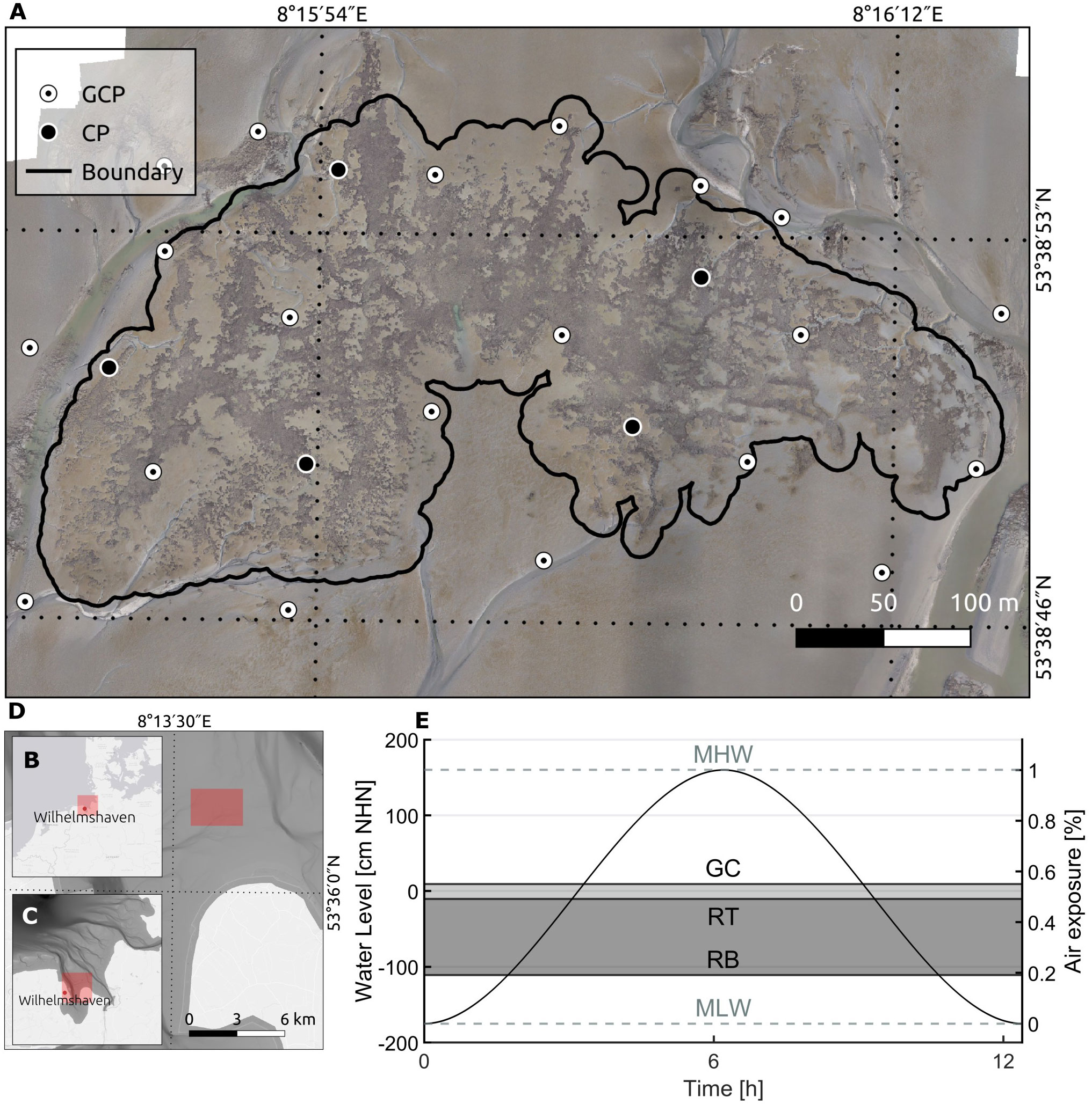
Figure 1 The upper map (A) shows an orthomosaic of the oyster reef at the Kaiserbalje with the distribution pattern of the ground control points (GCP) and check points (CP) for March 2022. The black contour line presents the rough reef boundary within the tidal creeks and a distance of 10 m to the oyster-identified area. Further, (B) a map of the Northern European coast, (C) the German Wadden Sea and (D) the Jade Bight are presented with the bathymetry of the Wadden Sea (Sievers et al., 2020). (E) The characteristic tide ranges between mean low water (MLW) of -1.75 m standard elevation zero (NHN, vertical datum in Germany) to mean high water (MHW) of 1.60 m NHN (WSV, 2022a). The oyster reef is located between the level of the reef top (RT) and bottom (RB). The growth ceiling (GC) indicates the upper growth limit at 55% air exposure, according to Walles (2015) and Ridge et al. (2015).

FIGURE 2

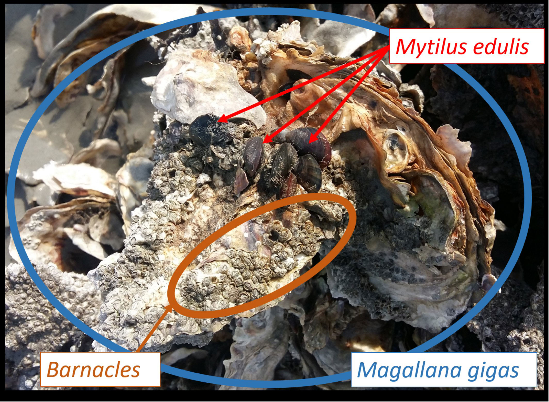
Figure 2 The coexistence of the Pacific oyster (Magallana gigas, blue ring) and the blue mussel (Mytilus edulis, red arrows) shapes the appearance of the Kaiserbalje and the roughness of the reef surface. Barnacles (the brown oval shape) commonly infest the surface of oyster shells, whereas the blue mussel finds its place between oysters.

2.2 Data collection

In six spring/autumn field campaigns, the topography of the Kaiserbalje was measured between October 2019 and March 2022 to obtain high-resolution data sets, employing an unoccupied, drone-style aerial vehicle (UAV) system. Every campaign comprised a two-hour flight mission of the reef, collecting between 1,099 and 2,010 images. Three-hour time windows limited the accessibility to the reef and working time during low tide conditions.

Recording of the study site was accomplished by a UAV (DJI Phantom 4 Pro), equipped with an integrated high-resolution RGB camera 1"-CMOS sensor capturing 20-megapixel images. This gimbal-mounted lightweight quadcopter used the Global Positioning System (GPS) of the US and the Global Navigation Satellite System (GLONASS) of Russia as on-board global navigation satellite system (GNSS) receivers. David and Schlurmann (2020) and Eltner et al. (2022) state accuracy of the built-in GNSS of 2-5 m. These first values estimate the camera location and orientation for the photogrammetric reconstruction influencing the DEM’s accuracy and classification performance. Field surveys were not conducted if the wind velocity exceeded a 7-8 m/s threshold since the drone failed to take off even though DJI states a maximum wind resistance of 10 m/s.

The flight app DroneDeploy (https://www.dronedeploy.com) was used for automatic flight missions, specifying a systematic strip-by-strip route with a constant velocity of 3 m/s and a recording frequency of one photo every three seconds. A sufficient front (80%) and side overlap (60%) ensured adequate data processing, according to Agisoft LLC (2019). Because low-resolution imagery cannot present small-scale features of biogenic oyster reefs (Ridge et al., 2020), a maximum flight altitude of 40 m was chosen to keep a sufficient ground sampling distance (GSD) of 1.2 cm. Since the Phantom only provided sub-meter positioning of the images, coordinates of defined ground control points (GCPs) on the ground of the field study were measured during the field surveys for indirect georeferencing to increase the absolute and relative accuracy of the DEMs in a cm-range in processing the UAV data set (Eltner et al., 2022). Further, this georeferencing contributed to avoiding doming effects in UAV imagery (Sanz-Ablanedo et al., 2018; Joyce et al., 2019; Pell et al., 2022).

In the three-hour time of aerial survey by UAV, up to 21 GCPs were distributed on the ground, evenly across the entire field area, particularly along the edges, corners, and as one line spanning the entire width of the reef. The GCPs used in this study were made of PVC tarpaulins and marked with a measuring cross. No GCPs were located at most 200 m from a neighbouring GCP, as recommended by Tonkin and Midgley (2016). Additionally, the coordinates of 1 to 6 check points (CP) were measured and used to validate the alignment accuracy in the SfM processing by subtracting the measured coordinates of the CPs from the estimated coordinates of the aligned point cloud. Due to time and accessibility limitations, 21 to 27 ground control and check points were distributed over an area of 270,000 m² (27 ha), resulting in a density of up to 0.2 CP/ha and 0.8 GCP/ha. This has been decided since the measuring on the intertidal mudflats and the oyster reef was challenging within the time limitations imposed by the tidal cycle. Other studies have applied varying numbers of CPs, ranging from zero (0 CP/ha) to twelve (4 CP/ha) validation points (Jaud et al., 2016; Brunier et al., 2020; David and Schlurmann, 2020), and sometimes as high as 80 (11.2 CP/ha, Brunetta et al. (2021)). Attaching the GCP underwater (i.e., in areas with tidal pools in the inner reef) encountered difficulties that would worsen the structure from motion (SfM) reconstruction and georeferencing due to reflection and refraction effects by the water (David et al., 2021; Casella et al., 2022; Pell et al., 2022), and thus, no GCP were placed when water still drained off in lower elevations. Water areas, especially tidal creeks and pools, affect elevation values and cause noise during the processing that was eliminated to avoid this issue. Oysters located underwater were excluded from the reef assessment due to challenges in accurate identification. A Stonex-9000-dGPS was used to measure the coordinates of GCPs and CPs with a horizontal accuracy of 0.008 m and a vertical accuracy of 0.015 m in Real-Time Kinematic (RTK) network mode.

The concerned authorities permitted all field investigations: Wadden Sea National Park Authority of Lower Saxony (NLPV) and the Agency for Coastal Defence, National Park and Marine Conservation Schleswig-Holstein (LKN.SH). Under the given regulations of the authorities, any effects on other species were minimised, and no disturbances were noticed during measurements. The drone pilot complied with the competency requirements of the EU regulation 2019/947 and was supported by one trained observer in the field.

2.3 Data processing

2.3.1 Structure from motion

Structure from motion (SfM) was applied to construct DEMs and orthomosaics by identifying characteristic key points in a series of multiview stereo imagery with known camera orientations and geotags (Westoby et al., 2012; Windle et al., 2022), providing robust 3D-structural metrics on a cm-scale (Ridge et al., 2023). The alignment, georeferencing, DEM generation (up to 210,000,000 points), and orthomosaics were processed within Agisoft Metashape^® (1.7.3, previously PhotoScan). The quality of the digital models depends on camera type, image resolution, level of image overlap, sun position, weather conditions and GCP distribution. The image quality is defined based on the sharpness of its most focused part (Tmuši ć et al., 2020). If the automatic assessment estimated the quality of the images below 0.5 units, they were refused for the alignment. Only one % was rejected for March 2021, and for the other surveys, the rate was less than one % or even zero %. All matches between GCPs and images were visually verified, and the camera alignment was optimised to ensure optimal georeferencing (Tmuši ć et al., 2020). The percentage of aligned images of all recorded images taken per survey was between 97% and 100% in the processing.

First, during the study period, the application of the GCPs was improved by increasing the number of GCPs and expanding the distribution across the entire reef. For this reason, the DEM of October 2019 could not be generated without any doming effects and, consequently, was removed from the analysis. These distortions led to non-acceptable data for further processing. Sufficiently good coverage of GCPs was established for the subsequent field campaigns, and the closer vicinity offered an appropriate georeferencing of the models. However, no more GCPs could be placed further north, as the northern part was hardly accessible due to strong currents in tidal creeks.

2.3.2 Classification

All DEM and orthomosaics were exported with a 5 cm/pixel resolution into QGIS (version 3.16 “Hannover”; qgis.org) to arrange the training data set for detecting oysters in the UAV imagery using a machine learning algorithm, as described below. This resolution was chosen to compromise the computing power (processing time and storage capacity) and the accuracy. This study integrated the oyster reef’s representative spectral and structural (roughness, slope and elevation) features into the training data set derived from the RGB bands and DEMs, respectively. Moreover, including a colour band derived from the orthomosaics as a roughness attribute demonstrates an enhanced classification success rate when incorporated into the training data. In this context, colour roughness refers to variances in the colour values between neighbouring pixels.

The supervised method Random Forest (RF) by Breiman (2001) was used, which is a suitable classifier for handling large data sets (Rodriguez-Galiano et al., 2012; Jhonnerie et al., 2015; Belgiu and Drăgut, 2016). The RF algorithm only identified oysters through the majority vote of an ensemble of multiple non-parametric classifications and decision trees (Breiman, 2001), each trained with a random selection of available attributes from a bootstrapped subset of the training data. The subset comprises around 64% of the training samples (in-bag samples) incorporated to train the trees. One-third remains of the training set (out-of-bag (OOB)) for unbiased and reliable estimation of the classification performance through an internal error rate (Breiman, 2001; Lawrence et al., 2006; Singh et al., 2017). The main advantages of the RF algorithm include high prediction accuracy, fast performance, and an ensemble decision of several hundreds of individual votes (Akar and Gungor, 2012; Rodriguez-Galiano et al., 2012; Näsi et al., 2018). However, one drawback of RF is that it works as a “black-box” classifier, not showing the rules applied to classify the data (Prasad et al., 2006; Rodriguez et al., 2014).

The prediction of the unclassified data was performed using the randomForest package (v. 4.7-1.1) (Liaw and Wiener, 2002) in R (v. 4.1.0) using RStudio (1.4.1717), along with the packages raster (v. 3.6-20), rgdal (v. 1.6-5), maptools (v. 1.1-6) and rgeos (v. 0.6-2). Most studies confirm stabilised classification results before the number of trees reaches 500 (Belgiu and Drăgut, 2016). We set m as 500 trees and n as 5 split variables.

Applying the OOB error, no further cross-validation nor testing was needed to estimate the classification performance (Prasad et al., 2006; Rodriguez-Galiano et al., 2012). Besides the OOB error, RF provides two additional variables to assess the importance of individual attributes for classification accuracy (Breiman, 2001). Firstly, the Mean Decrease Accuracy (MDA) is a factor that identifies the extent of the error in predicting the OOB data presenting how much accuracy the RF model loses when an attribute is excluded (Rodriguez-Galiano et al., 2012; Belgiu and Drăgut, 2016). A high MDA means a more substantial influence of the excluded attribute on the prediction (Bénard et al., 2022). Secondly, the Mean Decrease Gini (MDG) can describe how clearly the decision trees can split the data at the nodes (node impurity). The higher the MDG, the more critical the attribute is for the predictions (Welling et al., 2016). Like the MDA, one attribute was permuted and examined to what extent the best split weakens (Rodriguez-Galiano et al., 2012).

The classified output data was achieved with a success rate expressed as OOB error between 2.0% (March 2022) and 6.6% (September 2020), respectively. The OOB errors have reached a final equilibrium after 100-150 trees. The elevation and the roughness of both the DEM and the red channel of the RGB orthomosaic often had the highest impact on the MDA and MDG performance, i.e. the classification accuracy mainly depended on these factors. Figure 3 illustrates the coverage and the successful identification of the oyster reef.

FIGURE 3

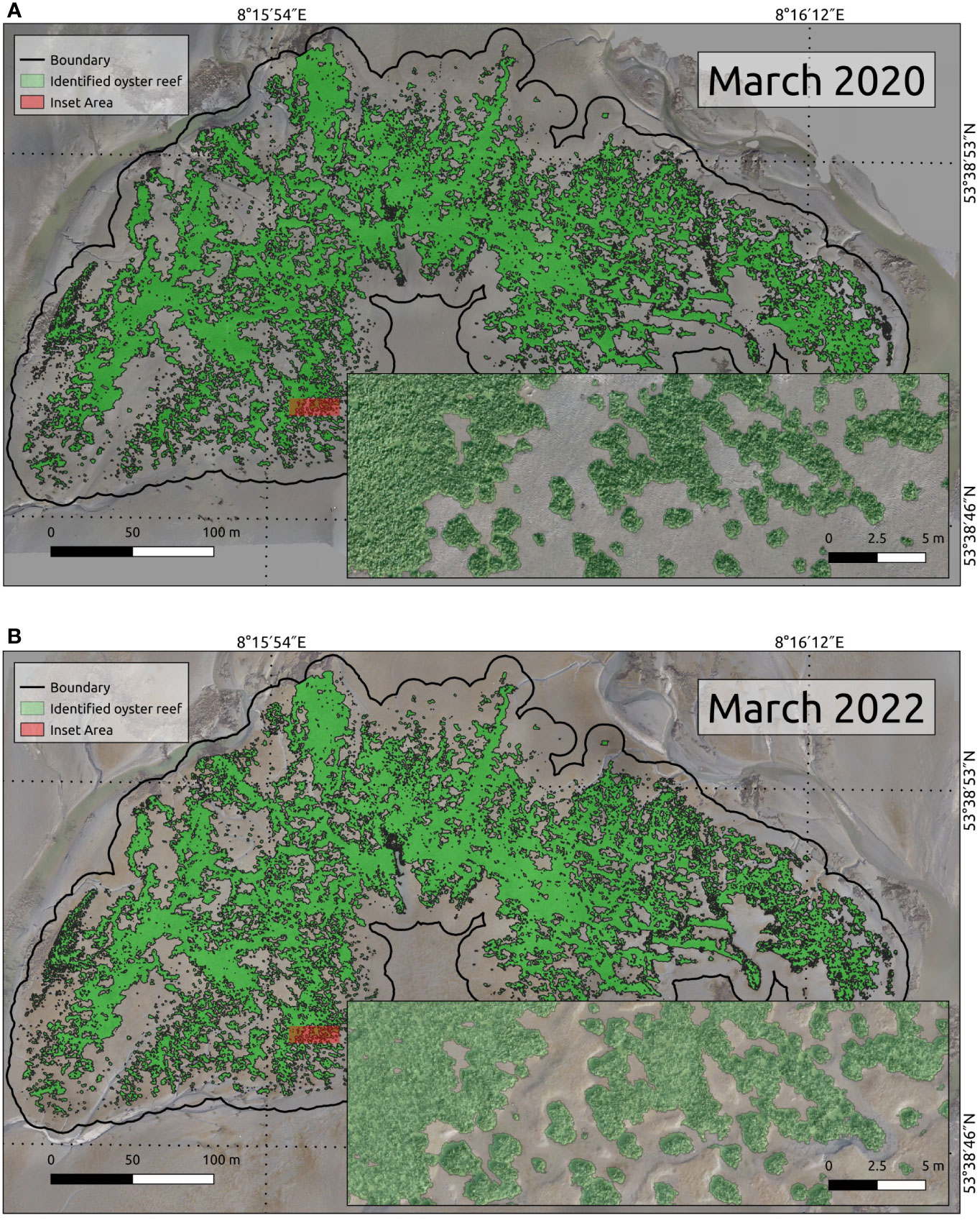
Figure 3 (A) and (B) showcase the oyster distribution (green coverage) determined by the Random Forest algorithm during the March surveys of 2020 and 2022. One can discern the precise classification of oyster populations by examining the insets (red area) of the main maps.

2.4 Error propagation

Determining small-scale changes in topography via remote sensing requires consideration of error propagation and uncertainties. Although the consequences of errors on volumetric results, previous marine and coastal studies have rarely analysed the propagation of errors, particularly for significant elevation changes. A few studies, e.g. Brunier et al. (2016), Jaud et al. (2016) and Duo et al. (2021), have determined the error propagation, considering the influence on volumetric changes in intertidal habitats. The identification and assessment of errors are not apparent in the photogrammetry for DEMs (Brasington et al., 2003). To determine the vertical uncertainty (σ_z) of DEMs, the errors of GPS measurements (σ_GPS) and the georeferencing performance in the photogrammetric processing (σ_CP) were combined as a propagating error. σ_z is an essential parameter in assessing the reliability of DEM data and based on σ_CP and σ_GPS. We recommend considering σ_CP and σ_GPS to derive the propagating error even if this approach might increasingly reduce information to the centimetre scale and, hence, increase the minimum level for detectable changes with statistical confidence. Our experience revealed that the “Marker accuracy” impact in Metashape was limited to the sub-millimetre scale for σ_CP. σ_CP accounts for the uncertainty associated with the georeferencing process of the DEM generation via CPs that were not applied in the georeferencing and optimisation procedures in the processing and used as independent validation points, as in Brasington and Smart (2003), Milan et al. (2007) and James et al. (2017). Neglecting errors associated with GPS measurements would result in underestimating the total uncertainty. CPs were not applied in the georeferencing and optimisation procedures in the processing.

The photogrammetric tool Metashape evaluated the vertical accuracy of the SfM-derived point clouds based on the coordinates of CPs and provided a single global uncertainty σ_CP as root mean square error (RMSE) covering the entire area of the DEM. RMSE is a standard statistical metric to assess the prediction errors (Milan et al., 2007) and presents the quadratic mean of the vertical differences Δz between the vertical estimated point cloud coordinates (z_estimated) and the measured (z_measured) coordinates of the CPs

$\begin{array}{ll}{\sigma }_{CP}=\sqrt{\frac{{\displaystyle {\sum }_{i=1}^n{(z_{i,estimated}-z_{i,measured})}^2}}{n}}& (1)\end{array}$

where n is the number of CPs. A total vertical RMSE of 2-3 times the GSD is expected to be achieved here, which can be considered well-accepted (Casella et al., 2020a). Under favourable conditions, a vertical accuracy of ~1-2 GSD can be achieved (Eltner et al., 2022). Analogously, the vertical RMSEs for the GCPs were also determined in Metashape, where the errors range between 0.2 cm and 0.6 cm. In contrast, the individual RMSEs of the CPs were in cm-range. In the following, the individual DEMs and other symbols are given with the format mmm-yy, where yy stands for the last two numbers of the corresponding year and mmm for the month. The σ_CP ranges between 1.9 (DEM_Mar-22), and 3.2 cm (DEM_Oct-21), whereas DEM_Sep-20 with three CPs produced the lowest error of 1.4 cm (~GSD, Table 1). Even though the GCPs were well- and uniformly distributed across the investigation field, they might not reduce the accuracy to zero but to a range of a few cm (Ventura et al., 2018; Chand and Bollard, 2021a).

The dGPS device estimated the vertical error using the vertical root mean square error (VRMSE) for each GCP measurement, which appeared to be higher than the manufacturer-specified device precision (s. subsection 2.2). The total vertical uncertainty of the GPS measurements σ_GPS is given as

$\begin{array}{ll}{\sigma }_{GPS}=\sqrt{\frac{{\displaystyle {\sum }_{i=1}^n{(VRMS{E}_i)}^2}}{n}}& (2)\end{array}$

and presents a global vertical uncertainty with n number of measurements. From the GPS measurement (Table 1), a σ_GPS between 1.9 cm (March 2021) and 2.5 cm (March 2020) was derived by the output of the dGPS device.

For each specific DEM, the overall vertical uncertainty σ_z,mmm−yy was calculated as the square root of the corresponding squares of the vertical uncertainties from both σ_CP and σ_GPS using the following formula

$\begin{array}{ll}{\sigma }_{z,mmm-yy}=\sqrt{{\sigma }_{GPS}^2+{\sigma }_{CP}^2}& (3)\end{array}$

where σ_z ranges between 2.7 (September 2020) and 3.9 cm (October 2021, Table 1).

TABLE 1

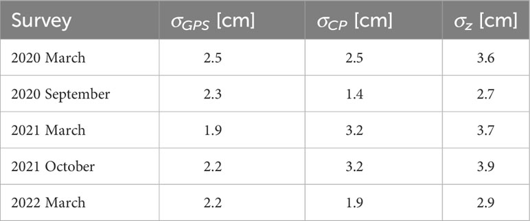
Table 1 The vertical uncertainty of the GPS measurement σ_GPS, the validation of the alignment σ_CP and the total vertical uncertainty σ_z.

When determining the volume growth and loss as well as the growth-related elevation changes of the reef structures over the study period, the total vertical uncertainty must be considered since this enables identifying areas with significant changes (Lane et al., 2003; James et al., 2017). When the slope is low, horizontal errors have a negligible effect on vertical surface differences (Wheaton et al., 2010), and therefore, the focus was only on vertical uncertainty. Combining the vertical uncertainties σ_z,mmm−yy of two DEMs, a common uncertainty σ_DoD that is equivalent to the standard deviation of the error was obtained

$\begin{array}{ll}{\sigma }_{\mathit{\text{DoD}}}=\sqrt{{\sigma }_{1,z,mmm-yy}^2+{\sigma }_{2,z,mmm-yy}^2}& (4)\end{array}$

for the DEMs of difference (DoD) that highlighted the geomorphological changes with a confidence level of 68% (Lane et al., 2003; Wheaton, 2008). This level conforms to a t-value of 1 associated with the student test that considers the propagation error into DoDs with a statistical basis, assuming a normal distribution of the errors (Taylor, 1997; Lane et al., 2003). This confidence level can be used as a threshold at which all values below it can be assumed as noise and above as minimum detectable change (Brasington et al., 2000).

Concerning the minimum change detection with a confidence level of 95%, the level of detection (LoD), a spatially uniform approach by Lane et al. (2003), was adopted to estimate significant changes. The LoD is a crucial metric and determines the minimum elevation change within DoDs (Wheaton et al., 2010; Lague et al., 2013; Winiwarter et al., 2021) that promises a statistically significant change. The LoD is the RMSE of the total vertical uncertainties σ_z,mmm−yy for two DEMs

$\begin{array}{ll}LoD=t\sqrt{{\sigma }_{1,z,mmm-yy}^2+{\sigma }_{2,z,mmm-yy}^2}& (5)\end{array}$

where t equals 1.96 under the t-distribution (Lane et al., 2003). Concerning the uncertainty of the elevation changes, the value of the σ_DoD or LoD was removed directly from the results, and all elevation changes below the LoD were considered “insignificant”. These changes are probably within the measurement error range and are treated as noise, whereas changes above the LoD are attributed to actual and significant geomorphological changes. In other words, a small LoD was preferred to detect smaller changes (Rengers et al., 2016). See subsection 2.5 on how to generate DoDs and yield volumetric changes with a certain confidence level related to σ_DoD or LoD. In this study, we analysed the influence of a confidence level on the results to discuss the credibility of small-scale changes without considering uncertainties.

The seasonal σ_DoD ranges between 4.5 and 5.4 cm, whereas the LoD varies between 8.8 and 10.6 cm (Table 2). Due to the smallest propagation errors in September 2020 and March 2022, the smallest uncertainty could be found for the DoD between September 2020 and March 2022, with a value of 4.0 cm and an LoD of 7.7 cm. The largest error occurred for DoD between March and October 2021, with 5.4 cm and 10.6 cm for σ_DoD and LoD, respectively.

TABLE 2

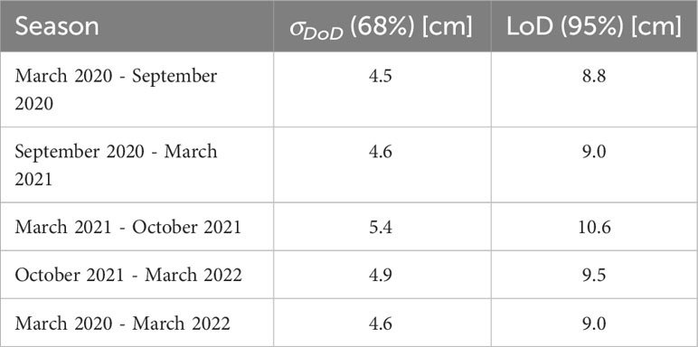
Table 2 The vertical uncertainty of the DEM with a confidence level of 68% (σ_DoD) and 95% (LoD).

To determine the volumetric uncertainty σ_V [m³] of a DoD with a confidence level of 68%, the corresponding uncertainty σ_DoD was multiplied by A_pixel and the number n of pixels of the area of either loss or increase.

$\begin{array}{ll}\sigma v=n·A_{\text{pixel}}·{\sigma }_{DoD}& (6)\end{array}$

According to a confidence of 95%, σ_DoD was replaced by LoD. Since the survey in March 2020 only had one CP, the corresponding RMSEs show low values (<GSD). To improve the reliability of the uncertainty of this survey, the errors were re-calculated and merged as a total vertical RMSE by the Leave-One-Out (LOO) method (Villanueva and Blanco, 2019; Casella et al., 2020b). This means that each GCP was excluded once and used as a CP in the model processing, where a copy of the original alignment was optimised within Metashape for each LOO configuration (nine in total).

2.5 Calculation of reef top elevation, area and volume change

All reef dimension calculations and the extraction of values were performed within QGIS. For each season survey, the reef area A_mmm−yy was determined from the total number of pixels n of the classified raster layer of the DEM multiplied by the pixel area A_pixel (0.0025 m²)

$\begin{array}{ll}{A}_{\text{mmm−yy}}=n·A_{\text{pixel}}& (7)\end{array}$

where yy and mmm indicate the year and the month. n was determined by subtracting the number of pixels with no values (“NODATA PIXEL COUNT”) from the total pixel count (“TOTAL PIXEL COUNT”). Both counts were yielded by the tool “Raster Layer Unique Values Report” in the “Processing Toolbox” of QGIS.

To determine the reef volume and bottom, we introduced a definition of the reef bottom, applying a lower limit of -0.6 m as a reference elevation z_ref in the computation. When considering the highest 99% of detected oysters, individuals were still found on this water depth for all maps. As most of the lower-lying oysters did not belong to the reef, the lowest 1% was excluded to eliminate individuals, clusters or other non-reef elements. The reef top (=maximum elevation point of the reef surface) was defined by identifying the 99.9^th percentile of oysters within the study field to exclude outliers and individuals outside the central reef structure. So far, no research has established specific upper and lower limits for an oyster reef based on the omission of a specific percentile. However, such an approach is not necessarily required when analysing smaller reefs but for larger reefs (> 100 m²) consisting of complex and interconnected reef components.

To describe the reef volume V_DEM,mmm−yy at the respective time of measurement, the sum of the elevation for each pixel that is given by subtracting the pixel elevation z_i value from z_ref was multiplied by A_pixel.

$\begin{array}{ll}{V}_{\text{DEM},mmm-yy}=A_{pixel}{\displaystyle \sum _{i=0}^{i=\text{max}}\left|z_{ref}-z_i\pm {\sigma }_z\right|}& (8)\end{array}$

If the volumes are computed with an uncertainty, σ_z (s. Equation 3) is appended to Equation 8. The tool “Raster Surface Volume” of the QGIS Processing toolbox was applied to find the volumes of the DEM raster (Input layer) where z_ref was used as the “Base level” and “Count Only Above Base Level” as a method. If considering the total vertical uncertainty σ_z, either σ_z is subtracted from the “Base level” or added to find the volumetric range. In addition to the volumes at the respective points in time, the volumetric changes were quantified between two survey times, where DoDs (Brasington et al., 2000; Wheaton et al., 2010) were determined by subtracting DEMs from each other pixel-by-pixel via the tool “Raster Calculator”.

$\begin{array}{ll}\text{DoD}=\text{DE}{\text{M}}_{\text{later},\text{mm}-\text{yyy}}-\text{DE}{\text{M}}_{\text{previous},\text{mmm}-\text{yy}}& (9)\end{array}$

The DoD raster output contains the elevation change of each pixel where positive values show a growth and negative a decrease in elevation. Subsequently, the volume changes were determined by multiplying the pixel size A_pixel with the elevation changes Δz in the DoD pixel-by-pixel (similar to Equation 8)

$\begin{array}{ll}{V}_{\text{increase}}=A_{\text{pixel}}{\displaystyle \sum _{i=0}^{i=\text{max}}(\mathrm{\Delta }{z}_i-{\sigma }_{DoD}·t)},\Delta z_i\ge {\sigma }_{DoD}·t& (10)\end{array}$

$\begin{array}{ll}{V}_{\text{Loss}}=A_{\text{pixel}}{\displaystyle \sum _{i=0}^{i=\text{max}}(\mathrm{\Delta }{z}_i+{\sigma }_{DoD}·t)},\left|\Delta z_i\right|\ge {\sigma }_{DoD}·t& (11)\end{array}$

where σ_DoD (s. Equation 9) is appended, and t equals either 1 or 1.96 when considering error propagation. To find the volumetric changes, the “Base level” was kept at zero, and either “Count Only Above Base Level” or “Count Only Below Base Level” were chosen in the tool “Raster Surface Volume” tool for volumetric growth and loss, respectively.

Figure 4 illustrates the previously described workflow to highlight the essential processing steps in this study.

FIGURE 4

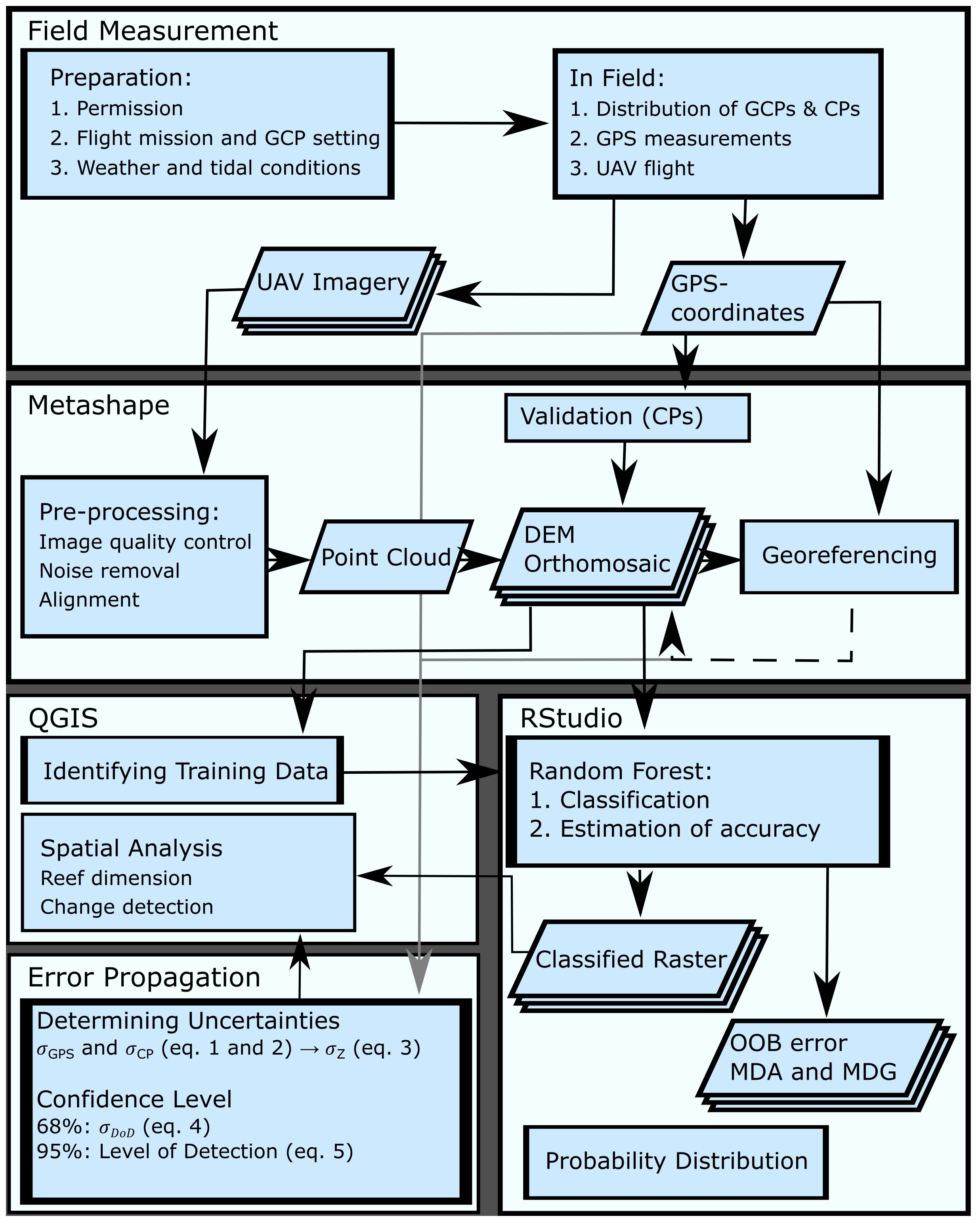
Figure 4 The workflow includes field measurements, photogrammetric processing in Metashape and QGIS, classification and statistical analysis in R, and error propagation analysis.

3 Results

3.1 Topographical changes

The elevation of the oyster reef top reaches an average of -0.15 ± 0.02 m NHN between 2020 and 2022, and most of the reef surface rises above the surrounding sediments (Figure 5). This allows the oyster reef to be distinguished from the surrounding tidal flats. The surrounding sediment within the reef boundary (Figure 1A) has an average elevation of -0.49 ± 0.02 m NHN, derived by the DEMs. Depths below -1.0 m NHN are located on the reef’s west and east sides, where tidal creeks were observed from the field measurements that did not fall dry entirely during low tide. The bottom of these tidal creeks pass along the reef edges and run into the bed of larger tidal creeks west and east of the reef. South to the reef, a shallower and narrower bed of a creek can be observed. In all tidal creeks, the water runs from north to south during the ebb and vice versa during the flood. Due to sediment deposition within the tidal creeks, higher surface elevations are observed than the actual bed elevation. When identifying the oyster reef, smaller patches were detected outside the reef, in and beyond the tidal creeks, but neglected in the analysis (<0.05 m²).

FIGURE 5

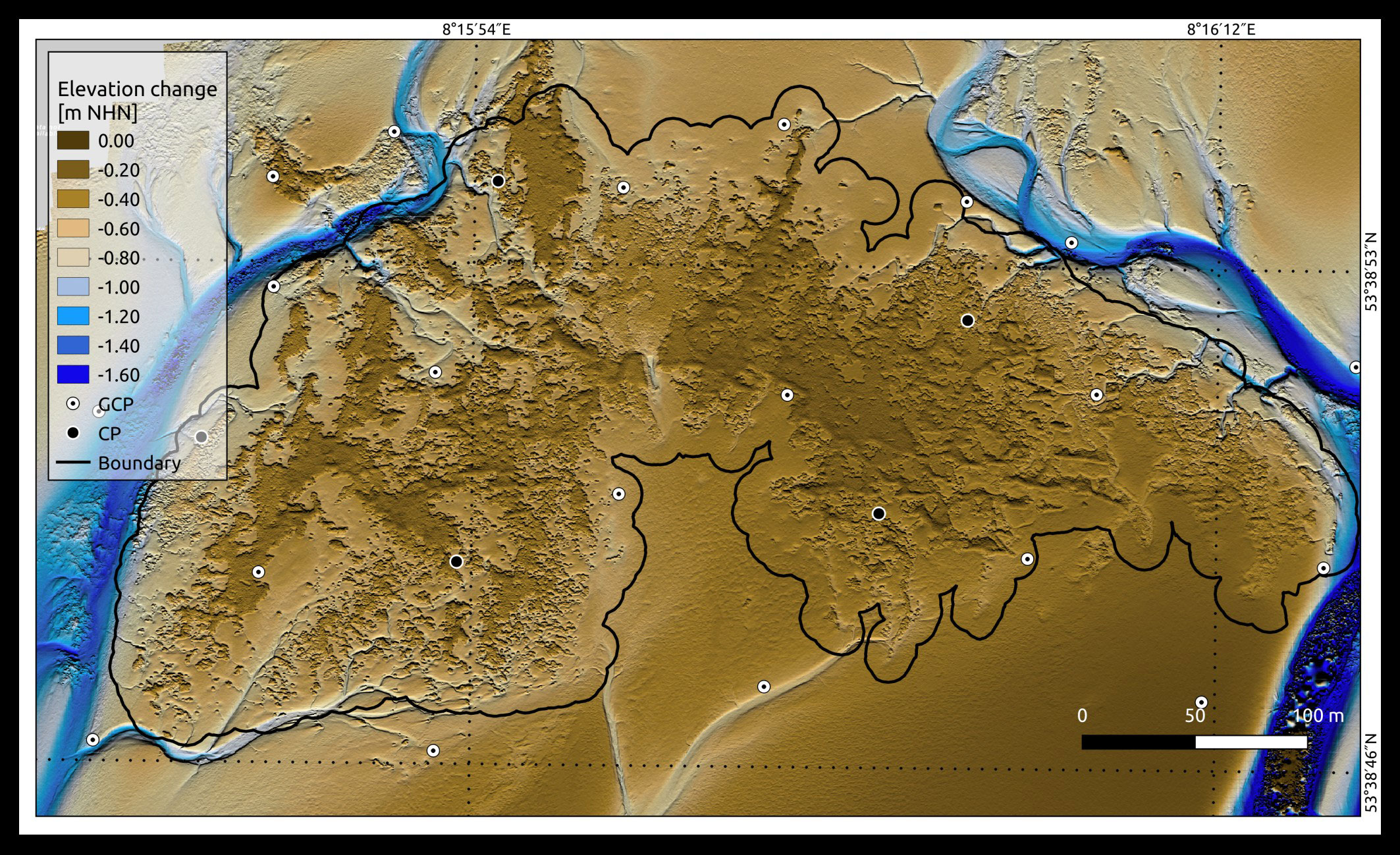
Figure 5 Digital elevation model (DEM) of the Kaiserbalje in March 2022 shows the actual elevation of the study site in m NHN. A hillshading effect was added to highlight the rough surfaces, providing a more natural spatial visualisation of the surface. Differences in height from 0.0 to -0.80 m NHN are represented in brown colours, and differences from -1.00 to -1.60 m NHN are illustrated in blue colours. The black contour line presents the rough reef boundary within the tidal creeks and a distance of 10 m to the oyster-identified area. The white points with the black dots present the ground control points (GCPs) distribution, and the black points illustrate the check points (CPs).

Primarily, the oyster reef comprises a lengthy central section surrounded by a transition zone and individual patches, as described in detail in Hitzegrad et al. (2022). The coverage of oysters on the tidal flats gradually diminishes from the central part towards the boundary of the reef, giving way to sediment patches that become spatially more dominant. In addition to these bare sediment areas, regions covered by biodeposits exist within the reef. In March 2022, the reef extended up to 550 m between the tidal creeks from west to east, and the reef width ranged between 100 and 400 m from north to south, with the narrowest stripe in the middle of the reef.

While the area determination is straightforward, defining the volume needs more attention due to the uncertainties caused by the GPS measurement and the photogrammetric alignment at a magnitude of 1.9 to 2.2 cm and 1.4 to 3.2 cm, respectively. The error propagation reveals elevations with uncertainties that eventually affect each survey’s volumes. Hence, presenting the volumetric results need to include these uncertainties in the following analysis. Maps of change detection with consideration of the confidence level are suitable for visualising the area of elevation changes (Figure 6).

Between March and September 2020 (Figure 6A), the reef grew vertically in a small area of 1,134 m² (3% of the initial reef area), where significant changes of 223 m² (<1%) were included, especially in the southwestern corner. However, erosion predominates in the north-western side over an area of approximately 5,500 m² (15%). In contrast, the reef could gain in growth on an area of >10,000 m² (27%) on the eastern side from September 2020 to March 2021 (Figure 6B). But minor 158 m² (<1%) areas at the edges close to the tidal creek were still eroded. Between March 2021 and March 2022 (Figure 6C), the reef could compromise the losses from the period between March 2020 and September 2020 on the western side (approx. 6,000 m², 18%) and the loss of the reef edge on the eastern side. From October 2021 to March 2022 (Figure 6D), reef expansion on 34 m² and only losses at the edges on the southeastern side (1,846 m², 5%) could be detected, including significant changes of an area of 271 m² (1%).

FIGURE 6

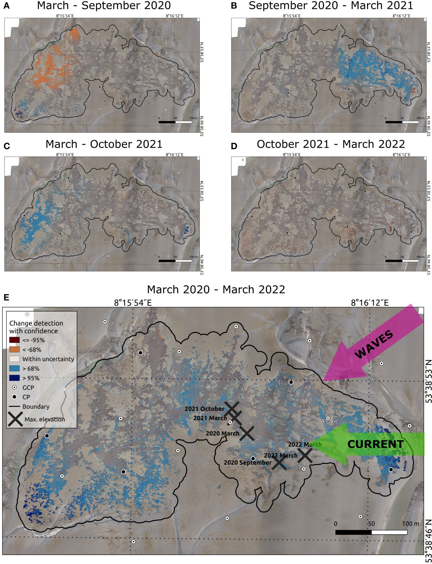
Figure 6 The subfigures (A–D) illustrate the seasonal and (E) the total vertical changes of the reef between surveys, divided into loss (brown) and increase (blue). (E) shows the topographical changes for the entire period from March 2020 to March 2022. The change detection with a confidence level of 68% is presented with light blue and brown colour and the significant changes with a confidence of 95% with a dark blue and brown colour. Both confidence levels correspond to a different minimum vertical change detection for each DoD (Table 2). Within the range of the uncertainty, the elevation changes are kept transparent, i. e. changes with a confidence of 68% and 95% are included above the uncertainty. The green and magenta arrows present the main direction of the current and waves, and the surveys’ maximum reef top elevations are marked with a black cross. The change detection without considering uncertainties are shown in the maps in Supplementary Material.

In summary, the largest areas of reef elevation increase were observed on the eastern side during the period of September 2020 and March 2021 and on the western side between March and October 2021. The largest area of elevation decrease was observed in the northwest and partially at the edges of the reef between March and September 2020. The DoD of March 2020 and March 2022 (Figure 6E) reveal that the oyster reef principally grew vertically over an area of 11,450 m² (30%) with confidence above 68%, especially at the east and southwest corners close to the tidal creeks. Significant growth in reef elevation was observed over an area of 1,298 m² (3%), whereas small reef parts (254 m², 1%) had decreased elevation along reef edges. The minimum and maximum vertical occurrence of oysters ranges between -1.26 ± 0.23 m and 0.00 ± 0.13 m NHN, including all identified oysters by the Random Forest algorithm.

The maximum surface elevation of the reef top ranged from -18.2 ± 2.7 cm NHN for DEM_Sep-20 to -12.8 ± 3.7 cm NHN for DEM_Mar-21, while the average surface elevation of the reef top was -0.15 ± 0.0 cm (47.8 ± 0.5% air exposure). In the final survey in May 2022, the maximum elevation reached -14.8 ± 3.9 cm NHN, resulting in a total vertical growth of 0.7 ± 4.6 cm over two years for the reef top. The largest increase in reef top elevation was observed within the period of September 2020 and March 2021, with an increase of 5.5 ± 4.6 cm (Figure 7). In contrast, the maximum elevation decreased for all other seasons, particularly between March and September 2020 (from -15.5 ± 3.6 cm NHN to -18.2 ± 2.7 cm NHN). The regression line in Figure 7 revealed a modest annual growth trend of 2.1 ± 13.9%, corresponding to 0.3 ± 3.6 cm/y over the two years for the reef top, with a coefficient of determination R² of 0.21, indicating a limited explanatory power of the model.

FIGURE 7

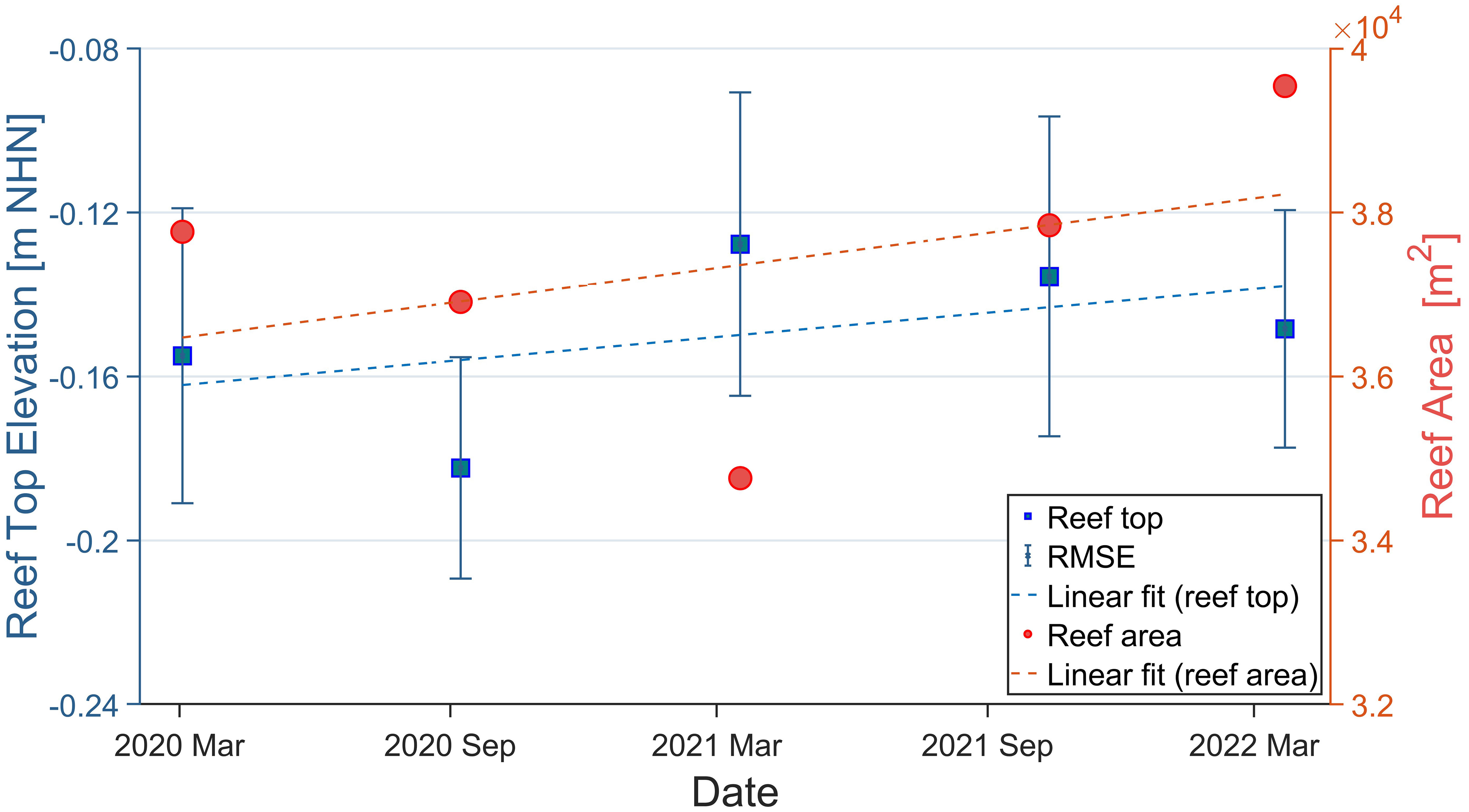
Figure 7 Development of the reef top elevation and the oyster reef area at the Kaiserbalje over the entire study period. The blue squares show the elevation at the time, with the associated vertical uncertainties (RMSE), and the red dots present the area size of the reef at the respective times. A regression line was drawn for both developments, with an R² value of 0.21 (elevation) and 0.16 (area).

The reef area development differed from the trend in elevation growth since the surface size had declined constantly from March 2020 (37,765 m²) to March 2021 (34,760 m²), resulting in a loss of 3,006 m² (Figure 7) that was followed by a steady growth until March 2022, the area growth compensates for the loss with 4,784 m² in the second half of the study period. During the study period, the reef area increased by 1,778 m², expanding from 37,765 m² to its maximum recorded size of 39,543 m² in March 2022, within our monitoring. Considering the regression line in Figure 7, the area experienced a growth of 889 m²/y. Since the coefficient of determination R² indicates a value of 0.16, no reliable trends should be concluded, given the limited explanatory power of the model.

Depending on the development of the reef elevation and area, the total reef volume extended from 8,046 ± 1,350 m³ in March 2020 to 9,370 ± 1,138 m³ in March 2022, with a total growth of 1,324 m³. Using -0.6 m as fixed reference elevation concerning the total vertical uncertainty σ_z (s. Equation 3), reef volume shows a clear increasing trend over the study period (Figure 8). Like the reef top elevation, the total reef volume decreased to a minimum of 7,561 ± 1,000 m³ in September 2020 but increased until September 2021 with a 9,374 ± 1,483 m³ volume. In contrast to the reef elevation and area, R² is higher with a value of 0.75, and the growth trend of 662 m³ or 7.9% is more credible for the reef volume.

While Figure 8 focuses on the volumes and net growth of the reef related to the time of the survey, the DoD approach provides insights into reef increase and loss. DoDs divide the volumetric change into loss and increase between two surveys, implying that DoDs do not present the volume at the exact measurement time. The increase or loss did not turn out to be constant, suggesting no seasonal effects on the reef during the study period of two years (Figure 9).

FIGURE 8

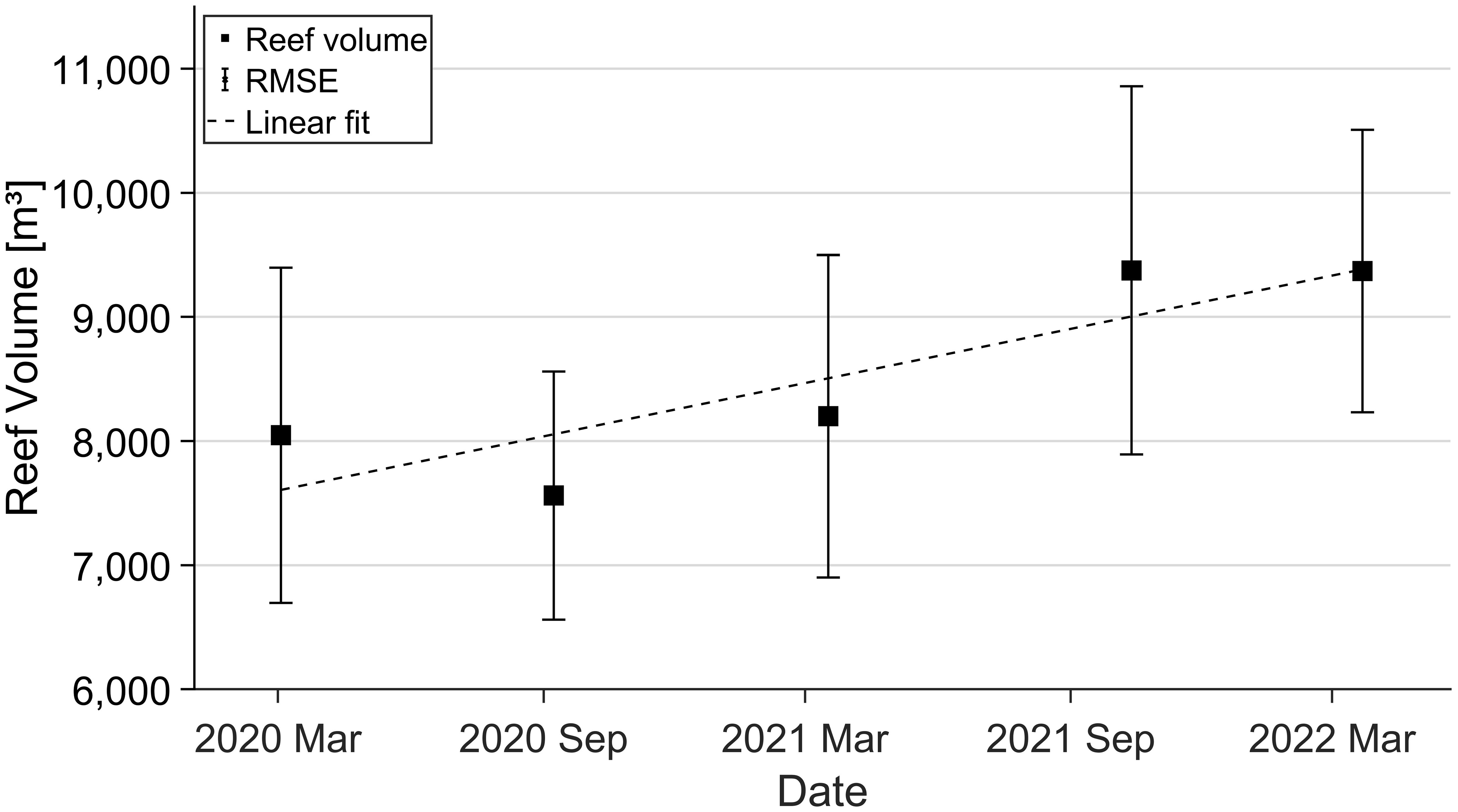
Figure 8 Mean volumetric oyster reef development over two years of observation. Error bars depict root mean square error (RMSE), and the dashed line indicates a linear regression with R² = 0.75.

FIGURE 9

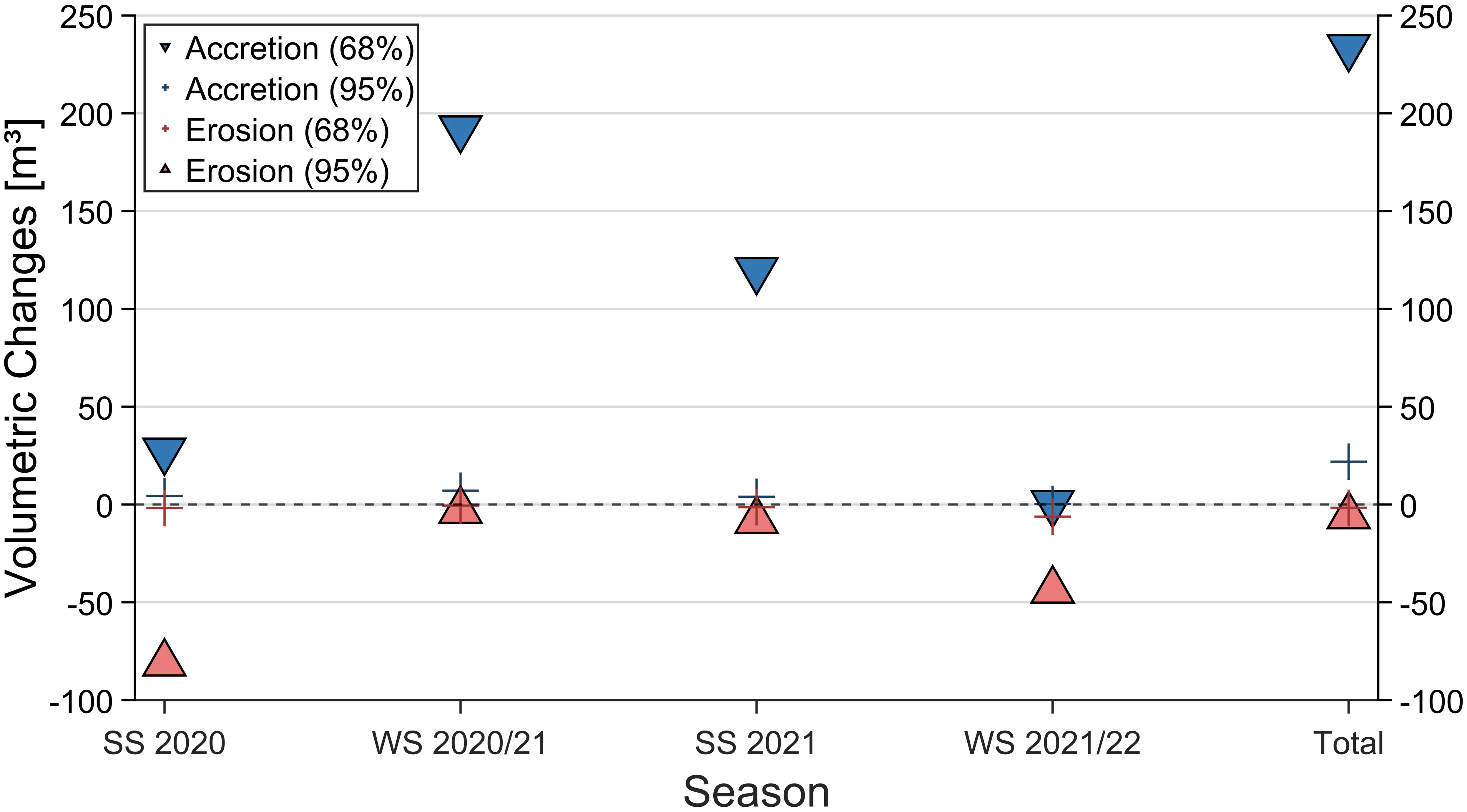
Figure 9 Volumetric changes illustrated according to their confidence level for each season and the total study period. The increase (blue) and loss (red) include the uncertainty σ_DoD (squares) and LoD (crosses) of the vertical changes, corresponding to a confidence level of 68% and 95%, respectively.

The results include the loss and increase calculated with a confidence level of 68% (σ_DoD, s. Equation 4) and a higher confidence level of 95% (LoD, s. Equation 5), highlighting the detection of geomorphological changes (Rengers et al., 2016) with confidence. Notably, the results on increase and loss considering LoD are one to two orders of magnitude smaller than those obtained with σ_DoD. No consideration of uncertainties would increase the resulting volumetric changes (s. Supplementary Material) and give more room for interpretations of the reef development.

Between March and September 2020, the reef experienced more loss than increase, followed by the period between September 2020 and October 2021, where the increase exceeded the amount of loss. However, in between October 2021 and March 2022, the loss volume rose relative to the increase. Regarding a confidence level of 95%, the total increase and loss yielded volumetric changes of 22 m³ and 2 m³, respectively, whereas a confidence level of 68% resulted in an increase of 234 m³ and a loss of 6 m³. This means the reef has a net gain of 20 m³ and 228 m³ for 95% and 68% confidence levels, respectively. If no confidence level is considered, the DoDs show broader areas of vertical changes, suggestive of potential growth tendencies on a broader scale. During the study period, the reef experienced a growth of 1,346 m³ covering 34,897 m² in the entire reef and a loss of 88 m³ over 5,348 m³ in the northwestern section when no uncertainties are considered.

3.2 Statistical assessment

The mean reef elevation of the Kaiserbalje ranged between -40.1 ± 2.7 cm (mean ± standard deviation) NHN (September 2020) and -35.7 cm NHN (October 2021), with a standard deviation σ between 9.3 and 10.5 cm, respectively (Figure 10). The mean elevation has shifted throughout the study time from -39.6 to -36.8 cm NHN. The probability distribution of the elevation demonstrates a consistent unimodal distribution with a well-defined peak.

FIGURE 10

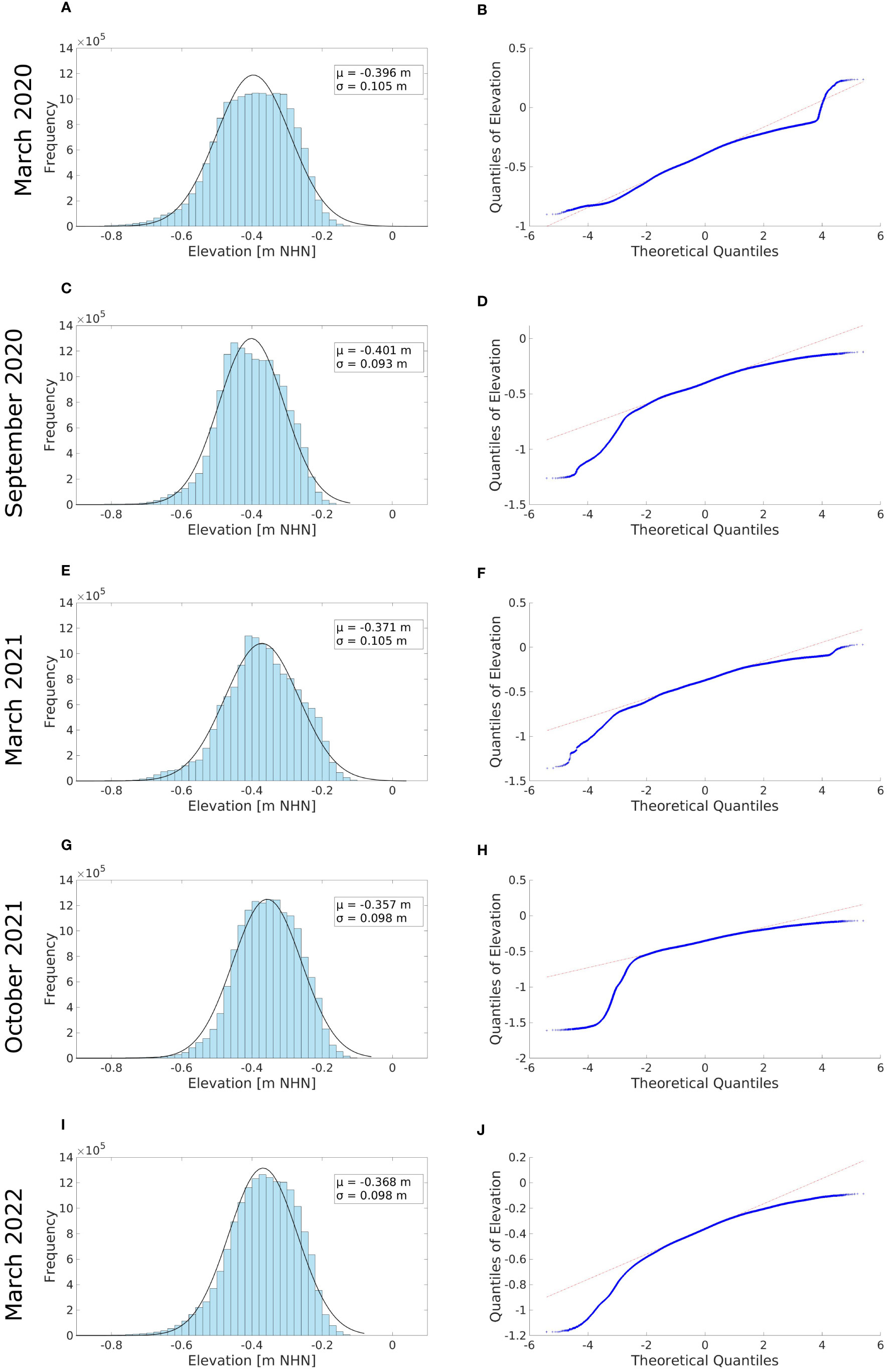
Figure 10 Left: Histograms of the probability distribution of the classified oysters’ elevations with the mean and standard deviation (A, C, E, G and I). Right: The quantile-quantile plots (Q-Q plots) show the probability distribution (B, D, F, H and J).

Regarding an oyster reef elevation distribution, a roughly symmetric distribution was found in March 2020 and for the subsequent surveys (Figures 10B, D, F, H, J), the elevation deviates from a normal distribution. On the one hand, a negative skewness (long left tails) indicates the presence of “extreme” elevation values for September 2020 to March 2022. On the other hand, the light right tails lead to the assumption that a potential upper limit exists. Walles et al. (2015) and Ridge et al. (2015) determined a growth limit of 55% air exposure. This aligns with our observations regarding the potential for further reef growth, extending to higher elevations and the subsequent upward shift of the distribution peak. Specifically, this growth limit corresponds to a 0.09 m NHN at the Kaiserbalje.

4 Discussion

This study’s results show a dynamic volumetric growth over the observation period of two years on the Kaiserbalje reef, with no evident seasonal effects. However, the magnitude of the results on the volumetric changes strongly depends on the confidence level introduced in the calculation (s. Equation 10 and Equation 11), considering the uncertainty in the elevation changes (Brasington et al., 2003; Wheaton et al., 2010; James et al., 2017). Thus, a thorough discussion of the volumetric changes must include error propagation, uncertainties, and understanding their impact on the results.

Unlike most previous studies in coastal monitoring, we consider error propagation and incorporate uncertainty in analysing small-scale changes affected by measurement and georeferencing errors. By accounting for these uncertainties, we can identify areas of changes with confidence in maps by applying DoDs, as in Wheaton et al. (2010) and James et al. (2020), and obtain more reliable results. Our approach follows a simple yet effective methodology to consider errors and achieve results with 68% and 95% confidence, as suggested by Taylor (1997) and Lane et al. (2003), striking a balance between precision and statistical robustness in determining volumetric changes. To date, no standard procedure or minimal guidance exists that includes propagating errors and uncertainties associated with change detection (Nourbakhshbeidokhti et al., 2019).

Lague et al. (2013) introduced a method including error propagation and spatially variable confidence by comparing (reference) point clouds using Multiscale Model to Model Cloud Comparison, M3C2. However, if reference measurements are missing, validation points such as check points can be applied to determine processing errors and estimate a global uncertainty covering the entire map as in our approach.

Studies with large elevation changes relative to vertical uncertainty yield more reliable results in terms of confidence since error propagation has a negligible effect on the minimum level of significant change detection. Most of the elevation changes in this study are within the range of uncertainties between 4.5 and 5.4 cm, especially for a confidence level of 95% (between 8.8 and 10.6 cm). Lower errors in measurement and processing should be pursued to achieve more significant change detection and increase the level of reliable information on topographical changes due to a low error tolerance for small-scale changes. Our results show the effect of uncertainties on volumetric changes and the effect of minor errors during measurements and processing. However, the uncertainties of DEMs and DoDs will unlikely reach values below 2-3 cm and 4-5 cm, respectively, due to the current limitations of the measurement tools. Similar studies (Brunier et al., 2016; Jaud et al., 2016; Duo et al., 2021) had RMSE values between 2 and 5 cm, which are also within our range of 2 and 4 cm. While this study focuses on the minimum detectable volumetric changes regarding confidence levels, other studies (Jaud et al., 2016; Brunetta et al., 2021) mainly address the overall patterns of volumetric changes, providing a range that considers uncertainty. While Jaud et al. (2016) highlights that uncertainties in DEMs limit the evaluation of sediment budgets, this work emphasises the importance of accounting for uncertainty to ensure credible results.

The Random Forest algorithm classifier has been convincing, featuring simple application and good classification results. The classification accuracy, expressed as OOB error, is below 7%, with the best (2%) results for March 2022. Higher classification results were accomplished because the roughness and texture of oyster reefs stood out on sandbanks, becoming an essential classification feature. The DEM’s high spatial resolution guaranteed the inclusion of the roughness that contributed crucially to the classification success. This aspect could be considered a standard attribute not just for oyster reefs but for other small-scale structures as well. Most studies applied only the spectral reflectance of surfaces as a training feature for RF.

4.1 Reef dynamic

A comparison of the development of reef areas with other studies is limited due to the small number of studies that differ in, e.g. site conditions, initial area sizes, and artificially constructed and not-constructed. Rodriguez et al. (2014) investigated the reef dimensions of artificially constructed reefs over fifteen years and stated an increase of 1.8 m²/y from approximately 15 m² to above 40 m² for younger reefs. A Pacific oyster study by Walles (2015) presented inventories of area sizes at the time of the measurements, ranging between 1,265 m² and 25,240 m². Still, no growth parameters for the area were reported. Kater and Baars (2003) revealed that the entire reef area in the Oosterschelde grew from ca. 250,000 m² (1980) to ca. 2,900,000 m² in 1990 and up to ca. 6,400,000 m² in 2000, leading to a yearly growth rate of 25.5% and 8.2% between 1980-1990 and 1990-2000, respectively.

The annual area growth of the reef at the Kaiserbalje was 2.3% (889 m²/y) between 2020 and 2022 and, hence, smaller than in the Oosterschelde, where the Pacific oyster was already introduced in 1964. Notably, direct comparisons of the Kaiserbalje with the Oosterschelde are difficult as the total oyster occurrence in the Oosterschelde consists of multiple reefs, and the environmental conditions vary between these sites. Probably due to the mature state of the Kaiserbalje reef, the constant expansion of the reef has stagnated and achieved a moderate balance of reef area after almost two decades of growth. First distinctive densities occurred in 2002 for the Kaiserbalje (Wehrmann, 2009).

Compared to surface area studies, more detailed investigations exist on the vertical growth of oyster reefs. The literature has shown that the reef’s surface and vertical growth depend on surface elevation or exposure time. When the reef top of the Pacific oyster reaches its growth ceiling, the increasing stress from air exposure will decelerate the vertical reef growth. Both in Walles (2015) and Ridge et al. (2015), a growth ceiling of 55% exposure time was identified for Pacific and Eastern oysters in the Oosterschelde (Netherlands) and North Carolina (US), respectively. For the same reefs in North Carolina, Ridge et al. (2015) could define a lower zero-growth boundary at an exposure time of 10% (mean low level). Walles et al. (2015) measured the uppermost point of oysters. They reported a growth ceiling between -1.68 m and -0.44 m (MSL) for the Pacific oyster, lower than the mean reef top elevation of -0.15 ± 0.02 m NHN of the Kaiserbalje reef.

Rodriguez et al. (2014) observed a vertical reef growth of 2.7 ± 0.7 cm/a for artificially constructed reefs between 10 and 14 years old, whereas two years old reefs showed a larger growth of 11.5 ± 1.4 cm/a. Similarly, Walles (2015) observed a faster vertical reef accretion rate for younger oyster reefs. From March 2020 to March 2022, the maximum reef top elevation has increased by about 0.6 cm yielding a mean annual growth rate of ~0.3 cm/a. This relatively low vertical growth is hypothesised to result from the reef’s maturity. Ridge et al. (2015) observed a correlation between the vertical reef growth and the elevation of American oyster reefs, for which they derived a description of an optimal growth zone between 40-50% of air exposure where the reefs experienced higher accretion rates. This study also analysed the correlation between vertical growth and elevation. Still, no apparent optimal growth zone could be detected about the air exposure for the Kaiserbalje reef. It is assumed that the reef will continue to grow over the entire reef area to an upper limit. As the current reef top elevation was determined at 47.8% air exposure, which is lower than the values of the growth ceiling in Walles et al. (2015) and Ridge et al. (2015), there is still about 24 cm vertical distance left to approach the growth ceiling, at about 55% air exposure. Based on the annual growth rate of ~0.3 cm/a, the reef top would need approximately 80 years to reach this maximum elevation, neglecting local sea level rise (SLR). The vertical growth may look different for distinct age phases of the reef and depend on the mean sea level (MSL). While oyster individuals in the central reef or other densely aggregated reef locations tend to grow straight up, individual oysters in the transition zone or on patches likely orient horizontally and spread more laterally. Ridge et al. (2017a) revealed that reef growth was aligned with MSL trends, with an increasing MSL promoting reef increase and a decreasing MSL leading to loss, indicating a dynamic equilibrium with sea level. This study observed volumetric growth changes, reporting temporal reef dynamics via UAV monitoring for the first time in the German Wadden Sea, demanding further validation and a longer investigation period to ensure these results. The elevation changes control the volumetric changes of oyster reefs, but only a few studies have described reef volumes and volumetric changes yet.

The volume-to-area ratio can serve as a relative benchmark for comparing other oyster reefs and, possibly, link the reef age. Between March 2020 and March 2022, the ratio of the Kaiserbalje reef varied between 0.21 m³/m² to 0.25 m³/m² (Figure 11) and similar ratios were found for constructed oyster reefs in the Oosterschelde (Walles et al., 2016b) and in North Carolina (Rodriguez et al., 2014). Nevertheless, the values only allow for a rough comparison due to the differences in volume definitions and type (natural and constructed reefs).

FIGURE 11

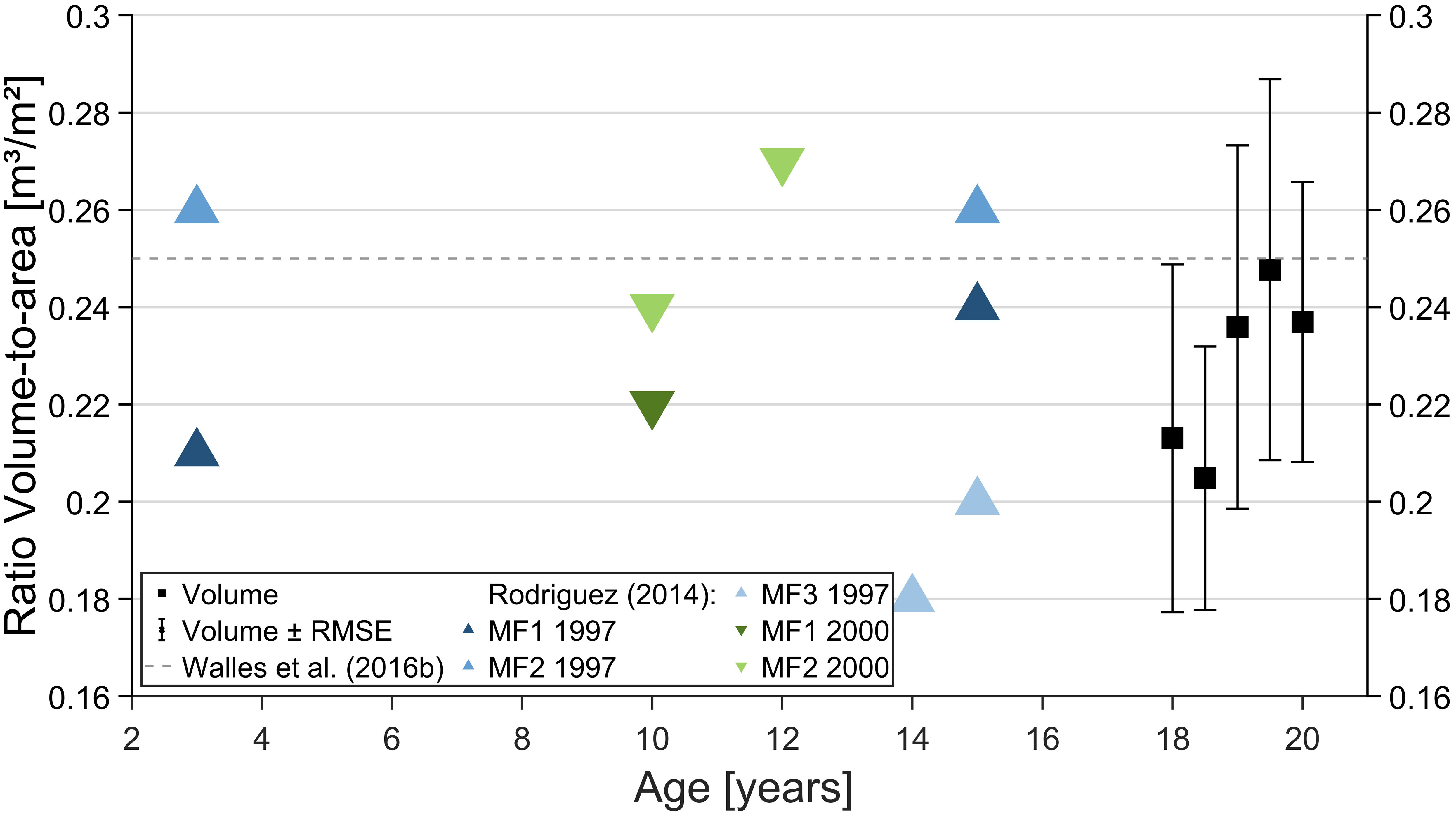
Figure 11 Volume-to-area ratio is presented with the corresponding root mean square error (RMSE, error bar) for all surveys in the study period (black squares). The dashed line presents the mean volume-to-area ratio of four constructed oyster reefs in the Oosterschelde (Walles et al., 2016a), and the triangles present the ratio for the constructed reefs established in 1997 (blue, upward-looking) and 2000 (green, downwardlooking triangle) in Rodriguez et al. (2014). When the field studies started in March 2020, the reef was at least 20 years old since the Kaiserbalje experienced the first notable increase in the oyster population in 2002 (Wehrmann, 2009). Note that the second values of MF1 and MF2 overlap.

The choice of a 68% or 95% confidence level aligns with statistical principles, ensuring that detected changes are likely to be real changes, not random fluctuations, and providing a robust basis for identifying meaningful geomorphological changes. Confidence levels help to focus on substantial changes while filtering out minor measurement and processing uncertainties. It ensures that only significant changes are considered for the analysis and interpretation. Applying DoDs with σ_DoD and LoD provides a practical approach to quantify the minimum volumetric changes between seasons or survey periods, as it accounts for the combined error propagation, unlike the previously reported method of individual total DEM volumes.

Considering uncertainties greatly impacts reef elevation and volume results in analysing small-scale changes of the same magnitude as the errors eliminate a large part of the detected changes. Higher confidence levels yield smaller detectable change areas. To increase the areas of change detection, reducing uncertainties in individual DEMs is necessary for geomorphological changes on a cm-scale. Our findings highlight the significant impact of propagation error on volumetric changes, with increase and loss values decreasing substantially when considering uncertainties. Without considering any errors, total increase and loss were 1,346 m³ and 88 m³, respectively, resulting in a total volumetric change of 1,258 m³. However, when applying a confidence level that accounts for uncertainty, the reef growth decreases to 234 m³ at a 68% confidence level and 22 m³ at 95%, a reduction to 17% and 0.3% of the volume without considering uncertainties, respectively. Similarly, loss values decrease to 6 m³ and 2 m³, corresponding to 7% and 2% of the volume without considering uncertainties. We can deduce that the scope for interpreting reef development decreases as the confidence level increases. Other studies have also shown that the degree of confidence and propagation error affects the area and volumes of volumetric changes, resulting in challenges when accurately determining changes (Jaud et al., 2016; Brunetta et al., 2021; Duo et al., 2021). Duo et al. (2021) found similar behaviour for volumetric changes as observed in this study. When the minimum detection level threshold is increased, there is a considerable decline in the proportion of detectable alterations within the area.

4.2 Abiotic stressors

The development of oyster reefs depends on numerous abiotic and biotic factors, such as hydrodynamic forces, salinity and temperature, which control growth and mortality (Chand, 2022) from the individual to the community scale. Successful reef growth depends on oysters’ spat fall, recruitment, growth and survival (Ridge et al., 2017a; Ridge et al., 2017b). Additionally, aerial exposure, salinity and water temperature are frequently mentioned as the primary physical drivers influencing oyster reef expansion (Baggett et al., 2015; Ridge et al., 2015; Walles et al., 2016a). Whereas according to Ridge et al. (2017a), salinity affects the growth pattern of oyster reefs, Palmer et al. (2021) stated that salinity is no main driver for limiting suitable areas. Herein, salinity measured at the lighthouse “Alte Weser” (WSV, 2022b) could not be identified as a stressor since the value remained relatively constant at 30.6 ± 1.5‰.

For further studies, we recommend analysing the reef development and the abiotic stressors, such as the temperature and salinity, since increased acidity endangers the calcification and development of oysters (Clements and Chopin, 2017; Ducker and Falkenberg, 2020), reducing oyster survival (Sanford et al., 2014) and limiting the reef growth.

Water temperature, however, is a primary driver affecting Pacific oysters’ reproduction, growth and population (Smaal et al., 2005; Hansen et al., 2023). Warmer temperatures promote reef expansion (Wehrmann et al., 2000; Diederich, 2005), while extreme temperatures around 30° C can weaken the oysters’ growth and survival (Bougrier et al., 1995), which was not observed during the study period (s. Supplementary Material). Successful spawning and settlement occur in the northern Wadden Sea between. July and September, where temperatures exceed 18° C for at least five to seven weeks (s. Supplementary Material), which were in the range of the minimum threshold of 17°-20° C for successful spawning (His et al., 1989; Castaños et al., 2009).

However, extended periods of cold temperatures can increase oyster mortality (Hansen et al., 2023). Nonetheless, no relationship was identified between the low water temperatures in winter and the reef area losses between September 2020 and March 2021. Besides low temperatures and ice drifts, storm events occurred during the winter seasons from October to March. The Federal Maritime and Hydrographic Agency (BSH) recorded 25 and 26 days of storm events in the North Sea for winter 2020-21 and 2021-22, respectively, that probably caused multiple inundations for over ten hours (Figure 12). However, only once, the reef was exposed to the air on the 7^th of February 2021 for more than ten hours (Figure 12 and Supplementary Material). During this extended low tide, the air temperature dropped below -3° C, and the water temperature around the reef ranged between 1° and 3° C. In particular, the upper layers of the oyster reef were exposed to stress over a longer period, where mortality probably increased. As Rodriguez et al. (2014) stated, extended exposure to air can lead to more stress, dehydration and deterioration of health, resulting in limited growth and increased mortality. Noteworthy was the twelve days of storm and one day of a heavy storm within 22 days in February 2022 (s. Supplementary Material) that had no or little effect on the reef development. In general, oysters are only exposed to air for a few hours while the oyster shells close and keep their moisture to survive during low tide. Hence, the increased dry fall and the cold temperatures likely caused increased mortality of oysters and a subsequent detachment from the reef in the winter of 2020/21, resulting in a decrease in surface area. Why the reef volume could still grow simultaneously is an open question.

FIGURE 12

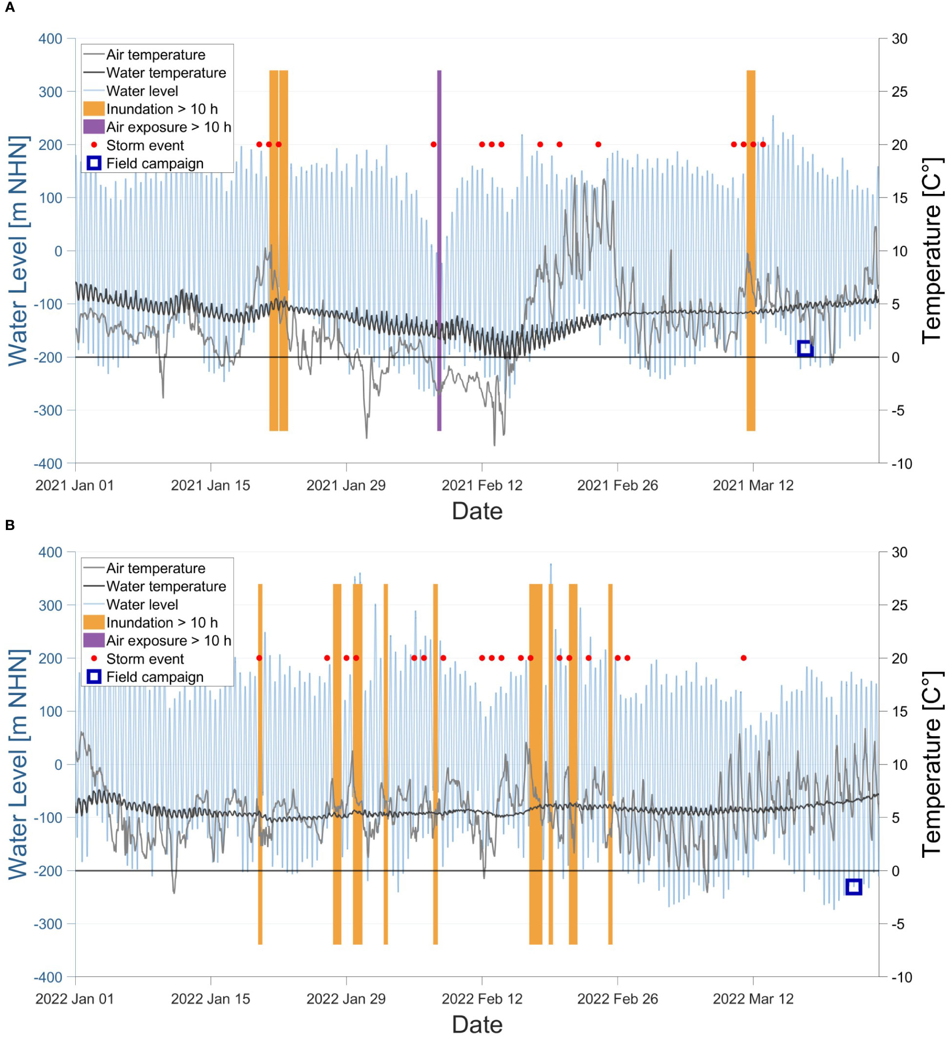
Figure 12 Potential stressors between January and March 2021 (A) and between January and March 2021 (B). The time histories of air (grey) and water (black) temperature and water level (blue) are shown here. Extreme water levels such as extended inundations (> ten hours, yellow) and low water (air exposure > ten hours of half of the reef, deep lilac) are presented as thick lines. Further, several storm events (red dots) occurred in winter. The entire water temperature profile can be found in Supplementary Material.

Global sea surface temperatures (SST) are expected to rise by 0.86° C between 2081-2100 compared to 1995-2014, projected by Coupled Model Intercomparison Project Phase 6 (CMIP6) models under the Shared Socio-economic Pathway 1-2.6 (SSP) (IPCC, 2022). This could lead to new habitats for Pacific oyster reefs and further expansion, but it could also cause increased mortality rates due to introducing new predators and diseases (Walles, 2015). Predicting how oyster reefs will adapt to this changing environment remains an active field of research.

In addition to ecological stress, oysters encounter constant hydrodynamic stress induced by waves and tidal currents, affecting their settlement and growth. Pacific oysters require suitable areas within the vertical growth zone, but rising sea levels may shift the vertical zone. Therefore, assessing if the reef’s growth rate can keep pace with local sea level rise is crucial. The current results show a yearly increase in the reef top elevation of 3.0 ± 36 mm/y, lagging the current rate of local SLR of 4.0 ± 1.53 mm/y in the North Sea from 1993 to 2009 (Wahl et al., 2013). By 2100, a recent SLR of 0.80 and 0.81 (median of RCP8.5) are projected for Cuxhaven and Hamburg, German North Sea coast cities, by Kopp et al. (2014) and Grinsted et al. (2015). This means that the current SLR rate will continue to increase, eventually outpacing the oyster reef growth rate identified here. However, these local SLR projections may be underestimated due to the potential partial representation of land subsidence (IPCC, 2023). For the next 80 years, the reef top could increase by 26 ± 286 cm and potentially keep pace with the SLR under favourable conditions, such as under SSP1-2.6, where an increase of 40 to 50 cm is estimated for the European oceans IPCC (2023). Our results represent only a two-year snapshot of the reef growth that must be validated through longer-term observations and examining oyster reefs in other locations. A comparison between oyster reef growth and local SLR beyond 2100 is subject to high uncertainties, and thus, it is not considered here.

4.3 Challenges in UAV monitoring and classification of oyster reefs

Low-cost monitoring with high-resolution drone data proved suitable for mapping and analysing reef growth and transferring to other coastal monitoring applications. The RGB bands and spatial resolution of UAVs provided sufficient information to classify the drone data successfully, despite the relatively flat and homogenous surfaces of tidal flats and oyster reefs. In the presence of other surface classes, the influence of seagrass, algae or other marine surfaces on classification success should be further investigated since the overlap of spectral features could result in lower classification success.

In previous studies, the focus was on detecting oyster reefs generally based only on multi- and hyperspectral (Schill et al., 2006; Choe et al., 2012; Le Bris et al., 2016) features or electromagnetic reflectance to detect and measure oyster reefs. Our results have proven that the RF approach can deliver high classification success in detecting small-scale changes in reef volume, even based on a consumer-grad drone with RGB sensors. Regarding temporal and spatial resolution, UAV monitoring is also convincing compared to satellite and airborne surveys, which lack the required structural information to identify small-scale reef characteristics (Ridge et al., 2023).

To investigate multiple oyster reefs in the German Wadden Sea on a regular base, the authors recommend investigating the possibilities of combining space-borne satellites and UAV monitoring for future monitoring of oyster reefs or other coastal ecosystems. Satellites can cover the entire German Wadden Sea, independing on personnel, while targeted missions with drones can fly over individual oyster reefs to ensure regular monitoring. Access to the investigation area was challenging and time-consuming, which led to limited spatial coverage and distribution of GCPs 0.8 GCP/ha and CPs (<0.2 CP/ha). However, if environmental and logistical conditions permit, increasing the number of CPs can improve the validity of σ_CP. In upcoming field campaigns, using an RTK drone may simplify the fieldwork and decrease the need for GCPs and CPs (Chen et al., 2023). Nonetheless, some GCPs and CPs are still necessary for accuracy enhancement (Štroner et al., 2020) and evaluation (Gonçalves and Henriques, 2015). For future investigations of reef surface elevation or volume changes, the authors recommend interpolating the error of the CPs over the entire area of interest to obtain a pointwise estimate of the uncertainty for the DEMs.

Our data provide a basis for small-scale analysis of oyster biomass, abundance and other ecological parameters that vary within the reef depending on the reef’s age and structural class (Hitzegrad et al., 2022). Due to the rough surface of oyster reefs, the spatial dimension has a crucial impact on the reef-flow interaction and surrounding sedimentation. Previous studies (Manis et al., 2015; Chowdhury et al., 2019) stated flow damping effects of oyster reefs, resulting in sediment trapping and stabilising effects. The DoD reveals a change in the sediment budget in the near and far-field of the reef, but it needs further investigation. As the rough oyster reefs dissipate the flow energy and dominate the changes in sedimentation processes, further investigations of the roughness effects on hydro- and morphodynamics are required.

So far, no studies have investigated and quantified the wave and current reduction under controlled laboratory conditions, except for Borsje et al. (2011) and Manis et al. (2015) who already tested the interaction between waves and oyster roughness in laboratories. However, a detailed investigation and quantification of roughness effects are still missing, especially on roughness effects on currents.

Within this study, we observed sediment accumulation around the reef but did not quantify it since it was outside the scope of this paper. Further research should focus on detecting sediment changes at the Kaiserbalje and comparison to other sites. The ecosystem engineering effects may contribute to coastal protection in the Wadden Sea by reducing the impact of waves and currents on the coast. After all, the flow damping and sediment stabilising need to be further investigated for their extent to evaluate the concrete contribution to coastal protection. It may prove that the Pacific oyster supports coastal protection as a nature-based solution (NbS) in the face of rising sea levels in the North Sea by sediment stabilisation. This can be of great importance when the oyster reefs rise at the same rate as the sea level and stabilise sediment in the longer term. To improve the reliability of the growth trends and limitations of the Kaiserbalje reef, further high-resolution monitoring of the reef via UAV over a longer period is highly recommended. Seasonal monitoring will deliver additional information on which periods the reef further grows and how temperature, air exposure, storm events and other abiotic factors influence the reef growth. So far, an ending of the horizontal expansion cannot be assumed since the surrounding sediment still offers space to settle on, and the reef could increase the coverage.

5 Conclusion

For the first time, seasonal volumetric changes of an oyster reef in the German Wadden Sea were precisely quantified to provide valuable growth parameters for estimating future reef expansion. Using low-cost monitoring through a consumer-grade UAV enabled the acquisition of high-resolution imagery, successfully classified by the Random Forest algorithm, resulting in accurate oyster maps. Despite successful change detection, the uncertainty of vertical growth challenged the quantification of small-scale changes. To address this, we adopted an approach of considering the error propagation through the processing, resulting in a high confidence (95%) of the reported significant changes. However, considering confidence levels reduced the area of detectable changes due to the increasing uncertainties and may eventually not represent the reef evolution sufficiently, resulting in vague interpretations. This study reveals that considering uncertainties ensures confident results, providing a minimum change detection of geomorphological changes. However, the results also show that large reef areas are often excluded from evaluating reef dynamics due to relatively high uncertainties. Even so, results without considering uncertainties can still describe reef dynamics and allow simple interpretations of reef development. As consumer-grade drones only cover small areas and the tide limits the flying time, space-borne systems could support monitoring oyster reefs on a larger scale. Furthermore, while consumer-grade drones offer the high spatial resolution necessary for accurate quantification of reef dynamics and expansion, space-borne systems may be valuable for monitoring oyster reefs on a larger scale, considering drones’ limited coverage and flying time. The approach employed in this study can be adapted for accurate and practicable monitoring of other ecosystems and contributes to marine ecology for sustainable coastal management strategies in the Wadden Sea.

The results indicate a net gain in reef area and volume, suggesting the potential of the reef to continue growing and keeping pace with the current local SLR. Given that the oyster reef or other hard substrate offer appropriate surfaces within the vertical growth zone, larvae can still settle, contributing to further reef expansion in all directions. While we could not define a specific growth ceiling (m NHN or air exposure) regarding reef top elevation for the Pacific oyster, the critical question remains whether the oyster reef will ever reach a growth limitation in light of the ongoing local SLR. While it is assumed that extended air exposure may have contributed to the observed decrease in area, no other stressors and seasonal effects influencing the volumetric growth were identified.

The promising results provided by this study make evident that long-term study periods are required for a better understanding of the growth dynamics and that validation with other oyster reefs to increase the robustness and reliability of results on the volumetric growth, particularly as elevations increase relative to uncertainties, is needed. Understanding the dynamics of oyster reefs is essential for effective coastal management, and this study contributes valuable insights to support such efforts.

Data availability statement

The raw data supporting the conclusions of this article will be made available by the authors, without undue reservation.

Author contributions

TH, MW, TS, MP, AW, and NG contributed to the conceptualisation. TH developed the methodology. TH, JH, KP, LB, AW, and MP carried out the investigation in the field studies. TH conducted the formal analysis. TH wrote the first draft of the manuscript and prepared visualisations. MW, MP, TS, AW and NG provided supervision. NG, AW, TS, and MP organised funding acquisition. NG was responsible for the project administration. All authors contributed to the article and approved the submitted version.

Funding

This project “BIVA-WATT” on which this work is based was funded by the Federal Ministry of Education and Research of Germany (BMBF) under the funding code 03KIS128. The publication of this article was funded by the Open Access Fund of Leibniz Universität Hannover.

Acknowledgments

The authors gratefully acknowledge the captain and crew of the FK Senckenberg for their logistics support and accommodation during the field campaigns and for keeping us safe on the North Sea. A special thank you goes to Torsten Janßen, who managed the field trips and guided us safely on the tidal flats. Regarding photogrammetric evaluation, we would like to thank Alexander Störmer and Dr. Bastian Steinhoff-Knopp (Institute of Physical Geography and Landscape Ecology, Hannover), who gave us hints for the UAV classification, and Prof. Anette Eltner (Institute of Photogrammetry and Remote Sensing, Dresden) for her valuable feedback concerning the analysis of error propagation. Additionally, we extend our appreciation to the students who supported us through their theses (Anne Eilrich, Katharina Michalak, Lennart Stukenborg, Lea Weiß, and Sylvi Junker) and as student assistants (Simon Bruns, Sebastian Köster, David Gläsner, Sharief Füglein, Nina Kohl, and Marten Beiermann). We acknowledge the Lower Saxon Wadden Sea National Park Authority (Wilhelmshaven) for their permits and cooperation.

Conflict of interest

The authors declare that the research was conducted in the absence of any commercial or financial relationships that could be construed as a potential conflict of interest.

Publisher’s note

All claims expressed in this article are solely those of the authors and do not necessarily represent those of their affiliated organizations, or those of the publisher, the editors and the reviewers. Any product that may be evaluated in this article, or claim that may be made by its manufacturer, is not guaranteed or endorsed by the publisher.

Supplementary material

The Supplementary Material for this article can be found online at: https://www.frontiersin.org/articles/10.3389/fmars.2023.1245926/full#supplementary-material

References

Adolph W., Jung R., Schmidt A., Ehlers M., Heipke C., Bartholomä A., et al. (2017a). Integration of terrasar-x, rapideye and airborne lidar for remote sensing of intertidal bedforms on the upper flats of norderney (german wadden sea). Geo-Marine Lett. 37, 193–205. doi: 10.1007/s00367-016-0485-z

CrossRef Full Text | Google Scholar

Adolph W., Schückel U., Son C. S., Jung R., Bartholomä A., Ehlers M., et al. (2017b). Monitoring spatiotemporal trends in intertidal bedforms of the german wadden sea in 2009–2015 with terrasar-x, including links with sediments and benthic macrofauna. Geo-Marine Lett. 37, 79–91. doi: 10.1007/s00367-016-0478-y

CrossRef Full Text | Google Scholar

Agisoft LLC (2019). Agisoft Metashape User Manual: Professional Edition, Version 1.5, 1.5 edn (St. Petersburg, Russia: Agisoft LLC).

Google Scholar

Akar Ö., Gungor O. (2012). Classification of multispectral images using random forest algorithm. J. Geodesy Geoinformation 1, 105–112. doi: 10.9733/jgg.241212.1

CrossRef Full Text | Google Scholar

Baggett L. P., Powers S. P., Brumbaugh R. D., Coen L. D., DeAngelis B. M., Greene J. K., et al. (2015). Guidelines for evaluating performance of oyster habitat restoration. Restor. Ecol. 23, 737–745. doi: 10.1111/rec.12262

CrossRef Full Text | Google Scholar

Beck M. W., Brumbaugh R. D., Airoldi L., Carranza A., Coen L. D., Crawford C., et al. (2011). Oyster reefs at risk and recommendations for conservation, restoration, and management. BioScience 61, 107–116. doi: 10.1525/bio.2011.61.2.5

CrossRef Full Text | Google Scholar

Behre K.-E. (2003). Eine neue meeresspiegelkurve für die südliche nordsee - transgressionen und regressionen in den letzten 10.000 jahren. Probleme der Küstenforschung im Südlichen Nordseegebiet 28, 9–64.

Google Scholar

Belgiu M., Drăgut L. (2016). Random forest in remote sensing: A review of applications and future directions. ISPRS J. Photogrammetry Remote Sens. 114, 24–31. doi: 10.1016/j.isprsjprs.2016.01.011

CrossRef Full Text | Google Scholar

Bénard C., Da Veiga S., Scornet E. (2022). Mean decrease accuracy for random forests: inconsistency, and a practical solution via the sobol-mda. Biometrika. doi: 10.1093/biomet/asac017

CrossRef Full Text | Google Scholar

Beukema J., Dekker R. (2005). Decline of recruitment success in cockles and other bivalves in the wadden sea: Possible role of climate change, predation on postlarvae and fisheries. Mar. Ecol. Prog. Ser. 287, 149–167. doi: 10.3354/meps287149

CrossRef Full Text | Google Scholar

Borsje B. W., van Wesenbeeck B. K., Dekker F., Paalvast P., Bouma T. J., van Katwijk M. M., et al. (2011). How ecological engineering can serve in coastal protection. Ecol. Eng. 37, 113–122. doi: 10.1016/j.ecoleng.2010.11.027

CrossRef Full Text | Google Scholar

Bougrier S., Geairon P., Deslous-Paoli J. M., Bacher C., Jonquières G. (1995). Allometric relationships and effects of temperature on clearance and oxygen consumption rates of crassostrea gigas (thunberg). Aquaculture 134, 143–154. doi: 10.1016/0044-8486(95)00036-2

CrossRef Full Text | Google Scholar

Bouma T. J., van Belzen J., Balke T., Zhu Z., Airoldi L., Blight A. J., et al. (2014). Identifying knowledge gaps hampering application of intertidal habitats in coastal protection: Opportunities & steps to take. Coast. Eng. 87, 147–157. doi: 10.1016/j.coastaleng.2013.11.014

CrossRef Full Text | Google Scholar

Brandt G., Wehrmann A., Wirtz K. W. (2008). Rapid invasion of crassostrea gigas into the german wadden sea dominated by larval supply. J. Sea Res. 59, 279–296. doi: 10.1016/j.seares.2008.03.004

CrossRef Full Text | Google Scholar

Brasington J., Langham J., Rumsby B. (2003). Methodological sensitivity of morphometric estimates of coarse fluvial sediment transport. Geomorphology 53, 299–316. doi: 10.1016/S0169-555X(02)00320-3

CrossRef Full Text | Google Scholar

Brasington J., Rumsby B. T., McVey R. A. (2000). Monitoring and modelling morphological change in a braided gravel-bed river using high resolution gps-based survey. Earth Surface Processes Landforms 25, 973–990. doi: 10.1002/1096-9837(200008)25:9{\textless}973::AID-ESP111{\textgreater}3.0.CO;2-Y

CrossRef Full Text | Google Scholar

Brasington J., Smart R. M. A. (2003). Close range digital photogrammetric analysis of experimental drainage basin evolution. Earth Surface Processes Landforms 28, 231–247. doi: 10.1002/esp.480

CrossRef Full Text | Google Scholar

Breiman L. (2001). Random forests. Mach. Learn. 45, 5–32. doi: 10.1023/A:1010933404324

CrossRef Full Text | Google Scholar

Brunetta R., Duo E., Ciavola P. (2021). Evaluating short-term tidal flat evolution through uav surveys: A case study in the po delta (Italy). Remote Sens. 13. doi: 10.3390/rs13122322

CrossRef Full Text | Google Scholar

Brunier G., Fleury J., Anthony E. J., Gardel A., Dussouillez P. (2016). Close-range airborne structure-from-motion photogrammetry for high-resolution beach morphometric surveys: Examples from an embayed rotating beach. Geomorphology 261, 76–88. doi: 10.1016/j.geomorph.2016.02.025

CrossRef Full Text | Google Scholar

Brunier G., Michaud E., Fleury J., Anthony E. J., Morvan S., Gardel A. (2020). Assessing the relationship between macro-faunal burrowing activity and mudflat geomorphology from uav-based structure-from-motion photogrammetry. Remote Sens. Environ. 241, 111717. doi: 10.1016/j.rse.2020.111717

CrossRef Full Text | Google Scholar

Brunier G., Oiry S., Gruet Y., Dubois S. F., Barillé L. (2022). Topographic analysis of intertidal polychaete reefs (sabellaria alveolata) at a very high spatial resolution. Remote Sens. 14, 307. doi: 10.3390/rs14020307

CrossRef Full Text | Google Scholar

Bungenstock F., Hertweck G., Hochstein M. L., Wehrmann A. (2021). Distribution pattern and controls of biosedimentary facies in backbarrier tidal flats of the central wadden sea (north sea). Z. der Deutschen Gesellschaft für Geowissenschaften 172, 409–428. doi: 10.1127/zdgg/2021/0248

CrossRef Full Text | Google Scholar

Burkett J. R., Hight L. M., Kenny P., Wilker J. J. (2010). Oysters produce an organic-inorganic adhesive for intertidal reef construction. J. Am. Chem. Soc. 132, 12531–12533. doi: 10.1021/ja104996y

PubMed Abstract | CrossRef Full Text | Google Scholar

Buscombe D., Goldstein E. B., Sherwood C. R., Bodine C., Brown J. A., Favela J., et al. (2022). Human–in–the–loop segmentation of earth surface imagery. Earth Space Sci. 9. doi: 10.1029/2021EA002085

CrossRef Full Text | Google Scholar

Büttger H., Nehls G., Witte S. (2011). High mortality of pacific oysters in a cold winter in the north-frisian wadden sea. Helgoland Mar. Res. 65, 525–532. doi: 10.1007/s10152-011-0272-1

CrossRef Full Text | Google Scholar

Casella V., Chiabrando F., Franzini M., Manzino A. M. (2020b). Accuracy assessment of a uav block by different software packages, processing schemes and validation strategies. ISPRS Int. J. Geo-Information 9, 164. doi: 10.3390/ijgi9030164

CrossRef Full Text | Google Scholar

Casella E., Collin A., Harris D., Ferse S., Bejarano S., Parravicini V., et al. (2017). Mapping coral reefs using consumer-grade drones and structure from motion photogrammetry techniques. Coral Reefs 36, 269–275. doi: 10.1007/s00338-016-1522-0

CrossRef Full Text | Google Scholar

Casella E., Drechsel J., Winter C., Benninghoff M., Rovere A. (2020a). Accuracy of sand beach topography surveying by drones and photogrammetry. Geo-Marine Lett. 40, 255–268. doi: 10.1007/s00367-020-00638-8

CrossRef Full Text | Google Scholar

Casella E., Lewin P., Ghilardi M., Rovere A., Bejarano S. (2022). Assessing the relative accuracy of coral heights reconstructed from drones and structure from motion photogrammetry on coral reefs. Coral Reefs 41, 869–875. doi: 10.1007/s00338-022-02244-9

CrossRef Full Text | Google Scholar

Castaños C., Pascual M., Camacho A. P. (2009). Reproductive biology of the nonnative oyster, crassostrea gigas (thunberg 1793), as a key factor for its successful spread along the rocky shores of northern patagonia, Argentina. J. Shellfish Res. 28, 837–847. doi: 10.2983/035.028.0413

CrossRef Full Text | Google Scholar

Chand S. (2022). Spatial dynamics of nearshore marine habitats from low altitude remote sensing for conservation and planning (Auckland: Dissertation, School of Science).

Google Scholar

Chand S., Bollard B. (2021a). Low altitude spatial assessment and monitoring of intertidal seagrass meadows beyond the visible spectrum using a remotely piloted aircraft system. Estuarine Coast. Shelf Sci. 255, 107299. doi: 10.1016/j.ecss.2021.107299

CrossRef Full Text | Google Scholar

Chand S., Bollard B. (2021b). Multispectral low altitude remote sensing of wild oyster reefs. Global Ecol. Conserv. 30, e01810. doi: 10.1016/j.gecco.2021.e01810

CrossRef Full Text | Google Scholar

Chen C., Tian B., Wu W., Duan Y., Zhou Y., Zhang C. (2023). Uav photogrammetry in intertidal mudflats: Accuracy, efficiency, and potential for integration with satellite imagery. Remote Sens. 15. doi: 10.3390/rs15071814

CrossRef Full Text | Google Scholar

Choe B.-H., Kim D.-j., Hwang J.-H., Oh Y., Moon W. M. (2012). Detection of oyster habitat in tidal flats using multi-frequency polarimetric sar data. Estuarine Coast. Shelf Sci. 97, 28–37. doi: 10.1016/j.ecss.2011.11.007

CrossRef Full Text | Google Scholar

Chowdhury M. S. N., Walles B., Sharifuzzaman S. M., Shahadat Hossain M., Ysebaert T., Smaal A. C. (2019). Oyster breakwater reefs promote adjacent mudflat stability and salt marsh growth in a monsoon dominated subtropical coast. Sci. Rep. 9, 8549. doi: 10.1038/s41598-019-44925-6

PubMed Abstract | CrossRef Full Text | Google Scholar

Clements J. C., Chopin T. (2017). Ocean acidification and marine aquaculture in north america: potential impacts and mitigation strategies. Rev. Aquaculture 9, 326–341. doi: 10.1111/raq.12140

CrossRef Full Text | Google Scholar

Collin A., Dubois S., Ramambason C., Etienne S. (2018). Very high-resolution mapping of emerging biogenic reefs using airborne optical imagery and neural network: the honeycomb worm ( sabellaria alveolata ) case study. Int. J. Remote Sens. 39, 5660–5675. doi: 10.1080/01431161.2018.1484964

CrossRef Full Text | Google Scholar

David C. G., Kohl N., Casella E., Rovere A., Ballesteros P., Schlurmann T. (2021). Structure-frommotion on shallow reefs and beaches: potential and limitations of consumer-grade drones to reconstruct topography and bathymetry. Coral Reefs 40, 835–851. doi: 10.1007/s00338-021-02088-9

CrossRef Full Text | Google Scholar

David C. G., Schlurmann T. (2020). Hydrodynamic drivers and morphological responses on small coral islands—the thoondu spit on fuvahmulah, the Maldives. Front. Mar. Sci. 7. doi: 10.3389/fmars.2020.538675

CrossRef Full Text | Google Scholar

Dehouck A., Lafon V., Baghdadi N., Roubache A. (2013). Potential of terrasar-x imagery for mapping intertidal coastal wetlands.

Google Scholar

de Paiva J. N. S., Walles B., Ysebaert T., Bouma T. J. (2018). Understanding the conditionality of ecosystem services: The effect of tidal flat morphology and oyster reef characteristics on sediment stabilization by oyster reefs. Ecol. Eng. 112, 89–95. doi: 10.1016/j.ecoleng.2017.12.020

CrossRef Full Text | Google Scholar

Diederich S. (2005). Invasion of Pacific oysters (Crassostrea gigas) in the Wadden Sea : competitive advantage over native mussels (Kiel: Dissertation, Christian-Albrechts-Universitat¨ zu Kiel).

Google Scholar

Dijkema K. S. (1997). Impact prognosis for salt marshes from subsidence by gas extraction in the wadden sea. J. Coast. Res. 13, 1294–1304.

Google Scholar

Doney S. C., Ruckelshaus M., Duffy J. E., Barry J. P., Chan F., English C. A., et al. (2012). Climate change impacts on marine ecosystems. Annu. Rev. Mar. Sci. 4, 11–37. doi: 10.1146/annurev-marine-041911-111611

CrossRef Full Text | Google Scholar

Ducker J., Falkenberg L. J. (2020). How the pacific oyster responds to ocean acidification: Development and application of a meta-analysis based adverse outcome pathway. Front. Mar. Sci. 7. doi: 10.3389/fmars.2020.597441

CrossRef Full Text | Google Scholar

Duffy J. P., Pratt L., Anderson K., Land P. E., Shutler J. D. (2018). Spatial assessment of intertidal seagrass meadows using optical imaging systems and a lightweight drone. Estuarine Coast. Shelf Sci. 200, 169–180. doi: 10.1016/j.ecss.2017.11.001

CrossRef Full Text | Google Scholar

Duo E., Fabbri S., Grottoli E., Ciavola P. (2021). Uncertainty of drone-derived dems and significance of detected morphodynamics in artificially scraped dunes. Remote Sens. 13. doi: 10.3390/rs13091823

CrossRef Full Text | Google Scholar

Eltner A., Hoffmeister D., Kaiser A., Karrasch P., Klingbeil L., Stöcker C., et al. (Eds.) (2022). UAVs for the environmental sciences: Methods and applications (Darmstadt: wbg Academic).

Google Scholar

Espriella M. C., Lecours V., C. Frederick P., V. Camp E., Wilkinson B. (2020). Quantifying intertidal habitat relative coverage in a florida estuary using uas imagery and geobia. Remote Sens. 12, 677. doi: 10.3390/rs12040677

CrossRef Full Text | Google Scholar

Fivash G. S., Stüben D., Bachmann M., Walles B., van Belzen J., Didderen K., et al. (2021). Can we enhance ecosystem-based coastal defense by connecting oysters to marsh edges? analyzing the limits of oyster reef establishment. Ecol. Eng. 165, 106221. doi: 10.1016/j.ecoleng.2021.106221

CrossRef Full Text | Google Scholar

Fodrie F. J., Rodriguez A. B., Baillie C. J., Brodeur M. C., Coleman S. E., Gittman R. K., et al. (2014). Classic paradigms in a novel environment: inserting food web and productivity lessons from rocky shores and saltmarshes into biogenic reef restoration. J. Appl. Ecol. 51, 1314–1325. doi: 10.1111/1365-2664.12276

CrossRef Full Text | Google Scholar

Folmer E. O., Drent J., Troost K., Büttger H., Dankers N., Jansen J., et al. (2014). Large-scale spatial dynamics of intertidal mussel (mytilus edulis l.) bed coverage in the german and dutch wadden sea. Ecosystems 17, 550–566. doi: 10.1007/s10021-013-9742-4

CrossRef Full Text | Google Scholar

Folmer E. O., Herlyn M., Markert A., Millat G., Troost K., Wehrmann A. (2017). Wadden Sea Quality Status Report: Beds of blue mussels and Pacific oysters (Wilhemshaven, Germany: Common Wadden Sea Secretariat).

Google Scholar

Gade M., Melchionna S., Stelzer K., Kohlus J. (2014). Multi-frequency sar data help improving the monitoring of intertidal flats on the german north sea coast. Estuarine Coast. Shelf Sci. 140, 32–42. doi: 10.1016/j.ecss.2014.01.007

CrossRef Full Text | Google Scholar

García-March J. R., Pérez-Rojas L., Garc´ıa-Carrascosa A. M. (2007). Influence of hydrodynamic forces on population structure of pinna nobilis l. 1758(mollusca: Bivalvia): The critical combination of drag force, water depth, shell size and orientation. J. Exp. Mar. Biol. Ecol. 342, 202–212. doi: 10.1016/j.jembe.2006.09.007

CrossRef Full Text | Google Scholar

Garvis S., Donnelly M., Hernandez E., Walters L., Weishampel J., Brockmeyer R. (2020). Remote sensing of live and dead intertidal oyster reefs using aerial photo interpretation in northeast florida. J. Coast. Conserv. 24. doi: 10.1007/s11852-020-00728-w

CrossRef Full Text | Google Scholar

Gmelin J. F. (1791). “Vermes,” in caroli a linnaei systema naturae per regna tria naturae, vol. 13 . Ed. Gmelin j.f. (Lipsiae: impensis Georg. Emanuel. Beer), 3021–3910. ed. 13. tome 1(6). g.e. beer, lipsiae [leipzig]Systema Naturae. Linneaeus (ed.).

Google Scholar

Gonçalves J. A., Henriques R. (2015). Uav photogrammetry for topographic monitoring of coastal areas. ISPRS J. Photogrammetry Remote Sens. 104, 101–111. doi: 10.1016/j.isprsjprs.2015.02.009

CrossRef Full Text | Google Scholar

Grabowski J., Brumbaugh R., Conrad R., Keeler A., Opaluch J., Peterson C., et al. (2012). Economic valuation of ecosystem services provided by oyster reefs. BioScience 632, 900–909. doi: 10.1525/bio.2012.62.10.10

CrossRef Full Text | Google Scholar

Grinsted A., Jevrejeva S., Riva R., Dahl-Jensen D. (2015). Sea level rise projections for northern europe under rcp8.5. Climate Res. 64, 15–23. doi: 10.3354/cr01309

CrossRef Full Text | Google Scholar

Grizzle R., Adams J. R., Walters L. J. (2002). Historical changes in intertidal oyster (crassostrea virginica) reefs in a florida lagoon potentially related to boating activities. J. Shellfish Res. 21, 749–756.

Google Scholar

Grizzle R., Ward K., Geselbracht L., Birch A. (2018). Distribution and condition of intertidal eastern oyster (crassostrea virginica) reefs in apalachicola bay florida based on high-resolution satellite imagery. J. Shellfish Res. 37, 1027. doi: 10.2983/035.037.0514

CrossRef Full Text | Google Scholar

Gutiérrez J. L., Jones C. G., Strayer D. L., Iribarne O. O. (2003). Mollusks as ecosystem engineers: the role of shell production in aquatic habitats. Oikos 101, 79–90. doi: 10.1034/j.1600-0706.2003.12322.x

CrossRef Full Text | Google Scholar

Hagen R., Plüß A., Schrage N., Dreier N. (2020). EasyGSH-DB: Themengebiet - synoptische Hydrodynamik (Hamburg, Germany: Bundesanstalt für Wasser). doi: 10.48437/02.2020.K2.7000.0004

CrossRef Full Text | Google Scholar

Hansen B. W., Dolmer P., Vismann B. (2023). Too late for regulatory management on pacific oysters in european coastal waters? J. Sea Res. 191, 102331. doi: 10.1016/j.seares.2022.102331

CrossRef Full Text | Google Scholar

Herlyn M. (2005). Quantitative assessment of intertidal blue mussel (mytilus edulis l.) stocks: combined methods of remote sensing, field investigation and sampling. J. Sea Res. 53, 243–253. doi: 10.1016/j.seares.2004.07.002

CrossRef Full Text | Google Scholar

His E., Robert R., Dinet A. (1989). Combined effects of temperature and salinity on fed and starved larvae of the mediterranean mussel mytilus galloprovincialis and the Japanese oyster crassostrea gigas. Mar. Biol. 100, 455–463. doi: 10.1007/BF00394822

CrossRef Full Text | Google Scholar

Hitzegrad J., Brohmann L., Pfennings K., Hoffmann T. K., Eilrich A. K., Paul M., et al. (2022). Oyster reef surfaces in the central wadden sea: Intra-reef classification and comprehensive statistical description. Front. Mar. Sci. 9. doi: 10.3389/fmars.2022.808018

PubMed Abstract | CrossRef Full Text | Google Scholar

Hogan S., Reidenbach M. A. (2022). Quantifying tradeoffs in ecosystem services under various oyster reef restoration designs. Estuaries Coasts 45, 677–690. doi: 10.1007/s12237-021-01010-4

CrossRef Full Text | Google Scholar

Hollander J., Blomfeldt J., Carlsson P., Strand Å. (2015). Effects of the alien pacific oyster (crassostrea gigas) on subtidal macrozoobenthos communities. Mar. Biol. 162, 547–555. doi: 10.1007/s00227-014-2604-6

CrossRef Full Text | Google Scholar

Hsu A. J., Kumagai J., Favoretto F., Dorian J., Guerrero Martinez B., Aburto-Oropeza O. (2020). Driven by drones: Improving mangrove extent maps using high-resolution remote sensing. Remote Sens. 12, 3986. doi: 10.3390/rs12233986

CrossRef Full Text | Google Scholar

IPCC (2018). Global Warming of 1.5°C: An IPCC Special Report on the impacts of global warming of 1.5°C above pre-industrial levels and related global greenhouse gas emission pathways, in the context of strengthening the global response to the threat of climate change, sustainable development, and efforts to eradicate poverty (New York: Cambridge University Press). doi: 10.1017/9781009157940

CrossRef Full Text | Google Scholar

IPCC (2021). Climate Change 2021: The Physical Science Basis. Contribution of Working Group I to the Sixth Assessment Report of the Intergovernmental Panel on Climate Change (New York: Cambridge University Press). press edn.

Google Scholar

IPCC (2022). Climate Change 2022: Impacts, Adaptation, and Vulnerability. Contribution of Working Group II to the Sixth Assessment Report of the Intergovernmental Panel on Climate Change (Cambridge, United Kingdom and New York, NY, USA: In Press).

Google Scholar

IPCC (2023). Climate change information for regional impact and for risk assessment. In Climate Change 2021 – The Physical Science Basis: Working Group I Contribution to the Sixth Assessment Report of the Intergovernmental Panel on Climate Change (Cambridge: Cambridge University Press), 1767–1926. IPCC. doi: 10.1017/9781009157896.014

CrossRef Full Text | Google Scholar

James M. R., Antoniazza G., Robson S., Lane S. N. (2020). Mitigating systematic error in topographic models for geomorphic change detection: accuracy, precision and considerations beyond off-nadir imagery. Earth Surface Processes Landforms 45, 2251–2271. doi: 10.1002/esp.4878

CrossRef Full Text | Google Scholar

James M. R., Robson S., Smith M. W. (2017). 3-d uncertainty-based topographic change detection with structure-from-motion photogrammetry: precision maps for ground control and directly georeferenced surveys. Earth Surface Processes Landforms 42, 1769–1788. doi: 10.1002/esp.4125

CrossRef Full Text | Google Scholar

Jaud M., Grasso F., Le Dantec N., Verney R., Delacourt C., Ammann J., et al. (2016). Potential of uavs for monitoring mudflat morphodynamics (application to the seine estuary, France). ISPRS Int. J. Geo-Information 5. doi: 10.3390/ijgi5040050

CrossRef Full Text | Google Scholar

Jhonnerie R., Siregar V. P., Nababan B., Prasetyo L. B., Wouthuyzen S. (2015). Random forest classification for mangrove land cover mapping using landsat 5 tm and alos palsar imageries. Proc. Environ. Sci. 24, 215–221. doi: 10.1016/j.proenv.2015.03.028

CrossRef Full Text | Google Scholar

Joyce K. E., Duce S., Leahy S. M., Leon J., Maier S. W. (2019). Principles and practice of acquiring drone-based image data in marine environments. Mar. Freshw. Res. 70, 952. doi: 10.1071/MF17380

CrossRef Full Text | Google Scholar

Jung R., Adolph W., Ehlers M., Farke H. (2015). A multi-sensor approach for detecting the different land covers of tidal flats in the german wadden sea — a case study at norderney. Remote Sens. Environ. 170, 188–202. doi: 10.1016/j.rse.2015.09.018

CrossRef Full Text | Google Scholar

Kater B. J., Baars J. (2003). Reconstructie van oppervlakten van litorale Japanse oesterbanken in de Oosterschelde in het verleden en een schatting van het huidig oppervlak (Texel, Netherlands; RIVO rapport (RIVO).

Google Scholar

Kopp R. E., Horton R. M., Little C. M., Mitrovica J. X., Oppenheimer M., Rasmussen D. J., et al. (2014). Probabilistic 21st and 22nd century sea-level projections at a global network of tide-gauge sites. Earth’s Future 2, 383–406. doi: 10.1002/2014EF000239

CrossRef Full Text | Google Scholar

Lague D., Brodu N., Leroux J. (2013). Accurate 3d comparison of complex topography with terrestrial laser scanner: Application to the rangitikei canyon (n-z). ISPRS J. Photogrammetry Remote Sens. 82, 10–26. doi: 10.1016/j.isprsjprs.2013.04.009

CrossRef Full Text | Google Scholar

Lane S. N., Westaway R. M., Murray Hicks D. (2003). Estimation of erosion and deposition volumes in a large, gravel-bed, braided river using synoptic remote sensing. Earth Surface Processes Landforms 28, 249–271. doi: 10.1002/esp.483

CrossRef Full Text | Google Scholar

Lawrence R. L., Wood S. D., Sheley R. L. (2006). Mapping invasive plants using hyperspectral imagery and breiman cutler classifications (randomforest). Remote Sens. Environ. 100, 356–362. doi: 10.1016/j.rse.2005.10.014

CrossRef Full Text | Google Scholar

Le Bris A., Rosa P., Lerouxel A., Cognie B., Gernez P., Launeau P., et al. (2016). Hyperspectral remote sensing of wild oyster reefs. Estuarine Coast. Shelf Sci. 172, 1–12. doi: 10.1016/j.ecss.2016.01.039

CrossRef Full Text | Google Scholar

Liaw A., Wiener M. (2002). Classification and regression by randomforest. R News 2, 18–22.

Google Scholar

Manis J. E., Garvis S. K., Jachec S. M., Walters L. J. (2015). Wave attenuation experiments over living shorelines over time: a wave tank study to assess recreational boating pressures. J. Coast. Conserv. 19, 1–11. doi: 10.1007/s11852-014-0349-5

CrossRef Full Text | Google Scholar

Markert A., Esser W., Frank D., Wehrmann A., Exo K.-M. (2013). Habitat change by the formation of alien crassostrea-reefs in the wadden sea and its role as feeding sites for waterbirds. Estuarine Coast. Shelf Sci. 131, 41–51. doi: 10.1016/j.ecss.2013.08.003

CrossRef Full Text | Google Scholar

Markert A., Wehrmann A., Kröncke I. (2010). Recently established crassostrea-reefs versus native mytilus-beds: differences in ecosystem engineering affects the macrofaunal communities (wadden sea of lower saxony, southern german bight). Biol. Invasions 12, 15–32. doi: 10.1007/s10530-009-9425-4

CrossRef Full Text | Google Scholar

Milan D. J., Heritage G. L., Hetherington D. (2007). Application of a 3d laser scanner in the assessment of erosion and deposition volumes and channel change in a proglacial river. Earth Surface Processes Landforms 32, 1657–1674. doi: 10.1002/esp.1592

CrossRef Full Text | Google Scholar

Mitchell I. M. (2006). In situ biodeposition rates of pacific oysters (crassostrea gigas) on a marine farm in southern tasmania (Australia). Aquaculture 257, 194–203. doi: 10.1016/j.aquaculture.2005.02.061

CrossRef Full Text | Google Scholar

Morrison M., Jones E. G., Consalvey M., Berkenbusch K. (2014). Linking marine fisheries species to biogenic habitats in New Zealand: A review and synthesis of knowledge, vol. no. 130 of New Zealand aquatic environment and biodiversity report (Wellington: Ministry for Primary Industries).

Google Scholar

Müller G., Stelzer K., Smollich S., Gade M., Adolph W., Melchionna S., et al. (2016). Remotely sensing the german wadden sea—a new approach to address national and international environmental legislation. Environ. Monit. Assess. 188, 595. doi: 10.1007/s10661-016-5591-x

PubMed Abstract | CrossRef Full Text | Google Scholar

Näsi R., Viljanen N., Kaivosoja J., Alhonoja K., Hakala T., Markelin L., et al. (2018). Estimating biomass and nitrogen amount of barley and grass using uav and aircraft based spectral and photogrammetric 3d features. Remote Sens. 10, 1082. doi: 10.3390/rs10071082

CrossRef Full Text | Google Scholar

Nehls G., Büttger H. (2007). Spread of the Pacific Oyster Crassostrea gigas in the Wadden Sea. Causes and consequences of a successful invasion (Husum).

PubMed Abstract | Google Scholar

Nieuwhof S., Herman P. M. J., Dankers N., Troost K., van der Wal D. (2015). Remote sensing of epibenthic shellfish using synthetic aperture radar satellite imagery. Remote Sens. 7, 3710–3734. doi: 10.3390/rs70403710

CrossRef Full Text | Google Scholar

Norling P., Kautsky N. (2007). Structural and functional effects of mytilus edulis on diversity of associated species and ecosystem functioning. Mar. Ecol. Prog. Ser. 351, 163–175. doi: 10.3354/meps07033

CrossRef Full Text | Google Scholar

Nourbakhshbeidokhti S., Kinoshita A. M., Chin A., Florsheim J. L. (2019). A workflow to estimate topographic and volumetric changes and errors in channel sedimentation after disturbance. Remote Sens. 11. doi: 10.3390/rs11050586

CrossRef Full Text | Google Scholar

OSPAR (2000). Quality Status Report 2000, Region II – Greater North Sea (London: OSPAR Commission).

Google Scholar

Palmer S. C., Barillé L., Kay S., Ciavatta S., Buck B., Gernez P. (2021). Pacific oyster (crassostrea gigas) growth modelling and indicators for offshore aquaculture in europe under climate change uncertainty. Aquaculture 532, 736116. doi: 10.1016/j.aquaculture.2020.736116

CrossRef Full Text | Google Scholar

Peine F., Bobertz B., Graf G. (2005). Influence if the blue mussel mytilus edulis (linnaeus) on the bottom roughness length (z0) in the south-western baltic sea. Baltica 18, 13–22.

Google Scholar

Pell T., Li J. Y. Q., Joyce K. E. (2022). Demystifying the differences between structure-frommotionsoftware packages for pre-processing drone data. Drones 6, 1–22. doi: 10.3390/drones6010024

CrossRef Full Text | Google Scholar

Piazza B. P., Banks P. D., La Peyre M. K. (2005). The potential for created oyster shell reefs as a sustainable shoreline protection strategy in louisiana. Restor. Ecol. 13, 499–506. doi: 10.1111/j.1526-100X.2005.00062.x

CrossRef Full Text | Google Scholar

Prasad A. M., Iverson L. R., Liaw A. (2006). Newer classification and regression tree techniques: Bagging and random forests for ecological prediction. Ecosystems 9, 181–199. doi: 10.1007/s10021-005-0054-1

CrossRef Full Text | Google Scholar

Reise K., Buschbaum C., Büttger H., Rick J., Wegner K. M. (2017). Invasion trajectory of pacific oysters in the northern wadden sea. Mar. Biol. 164, 68. doi: 10.1007/s00227-017-3104-2

PubMed Abstract | CrossRef Full Text | Google Scholar

Rengers F. K., Tucker G. E., Moody J. A., Ebel B. A. (2016). Illuminating wildfire erosion and deposition patterns with repeat terrestrial lidar. J. Geophysical Research: Earth Surface 121, 588–608. doi: 10.1002/2015JF003600

CrossRef Full Text | Google Scholar

Ridge J. T., DiGiacomo A. E., Rodriguez A. B., Himmelstein J. D., Johnston D. W. (2023). Comparison of 3d structural metrics on oyster reefs using unoccupied aircraft photogrammetry and terrestrial lidar across a tidal elevation gradient. Remote Sens. Ecol. Conserv 9, 501–511. doi: 10.1002/rse2.324

CrossRef Full Text | Google Scholar

Ridge J. T., Gray P. C., Windle A. E., Johnston D. W. (2020). Deep learning for coastal resource conservation: automating detection of shellfish reefs. Remote Sens. Ecol. Conserv. 6, 431–440. doi: 10.1002/rse2.134

CrossRef Full Text | Google Scholar

Ridge J. T., Rodriguez A. B., Fodrie F. J. (2017a). Evidence of exceptional oyster-reef resilience to fluctuations in sea level. Ecol. Evol. 7, 10409–10420. doi: 10.1002/ece3.3473

PubMed Abstract | CrossRef Full Text | Google Scholar

Ridge J. T., Rodriguez A. B., Fodrie F. J. (2017b). Salt marsh and fringing oyster reef transgression in a shallow temperate estuary: Implications for restoration, conservation and blue carbon. Estuaries Coasts 40, 1013–1027. doi: 10.1007/s12237-016-0196-8

CrossRef Full Text | Google Scholar

Ridge J. T., Rodriguez A. B., Joel Fodrie F., Lindquist N. L., Brodeur M. C., Coleman S. E., et al. (2015). Maximizing oyster-reef growth supports green infrastructure with accelerating sea-level rise. Sci. Rep. 5, 14785. doi: 10.1038/srep14785

PubMed Abstract | CrossRef Full Text | Google Scholar

Rodriguez A. B., Fodrie F. J., Ridge J. T., Lindquist N. L., Theuerkauf E. J., Coleman S. E., et al. (2014). Oyster reefs can outpace sea-level rise. Nat. Climate Change 4, 493–497. doi: 10.1038/NCLIMATE2216

CrossRef Full Text | Google Scholar

Rodriguez-Galiano V. F., Ghimire B., Rogan J., Chica-Olmo M., Rigol-Sanchez J. P. (2012). An assessment of the effectiveness of a random forest classifier for land-cover classification. ISPRS J. Photogrammetry Remote Sens. 67, 93–104. doi: 10.1016/j.isprsjprs.2011.11.002

CrossRef Full Text | Google Scholar

Román A., Tovar-Sánchez A., Olivé I., Navarro G. (2021). Using a uav-mounted multispectral camera for the monitoring of marine macrophytes. Front. Mar. Sci. 8. doi: 10.3389/fmars.2021.722698

CrossRef Full Text | Google Scholar

Sanford E., Gaylord B., Hettinger A., Lenz E. A., Meyer K., Hill T. M. (2014). Ocean acidification increases the vulnerability of native oysters to predation by invasive snails. Proc. R. Soc. B: Biol. Sci. 281, 20132681. doi: 10.1098/rspb.2013.2681

CrossRef Full Text | Google Scholar

Sanz-Ablanedo E., Chandler J., Rodríguez-Pérez J., Ordóñez C. (2018). Accuracy of unmanned aerial vehicle (uav) and sfm photogrammetry survey as a function of the number and location of ground control points used. Remote Sens. 10, 1606. doi: 10.3390/rs10101606

CrossRef Full Text | Google Scholar

Schill S., Porter D., Coen L., Bushek D., Vincent J. (2006). Development of an automated mapping technique for monitoring and managing shellfish distributions: A final report submitted to: The noaa/unh cooperative institute for coastal and estuarine environmental technology (ciceet) (Port Norris, NJ, USA: The NOAA/UNH Cooperative Institute for Coastal and Estuarine Environmental Technology (CICEET)).

Google Scholar

Schmidt A. (2009). Gefährdungspotential der eulitoralen Miesmuschelbänke im Niedersächsischen Wattenmeer durch die Bioinvasion der Pazifischen Auster (Crassostrea gigas) (Bremen: Dissertation, Universität Bremen).

Google Scholar

Schmidt A., Wehrmann A., Dittmann S. (2008). Population dynamics of the invasive pacific oyster crassostrea gigas during the early stages of an outbreak in the wadden sea (Germany). Helgoland Mar. Res. 62, 367–376. doi: 10.1007/s10152-008-0125-8

CrossRef Full Text | Google Scholar

Schulte D. M., Burke R. P., Lipcius R. N. (2009). Unprecedented restoration of a native oyster metapopulation. Science 325, 1124–1128. doi: 10.1126/science.1176516

PubMed Abstract | CrossRef Full Text | Google Scholar

Scyphers S. B., Powers S. P., Heck K. L. Jr, Byron D. (2011). Oyster reefs as natural breakwaters mitigate shoreline loss and facilitate fisheries. PloS One 6, e22396. doi: 10.1371/journal.pone.0022396

PubMed Abstract | CrossRef Full Text | Google Scholar

Seymour A. C., Ridge J. T., Rodriguez A. B., Newton E., Dale J., Johnston D. W. (2018). Deploying fixed wing unoccupied aerial systems (uas) for coastal morphology assessment and management. J. Coast. Res. 34, 704. doi: 10.2112/JCOASTRES-D-17-00088.1

CrossRef Full Text | Google Scholar

Sharma S., Goff J., Cebrian J., Ferraro C. (2016b). A hybrid shoreline stabilization technique: Impact of modified intertidal reefs on marsh expansion and nekton habitat in the northern gulf of Mexico. Ecol. Eng. 90, 352–360. doi: 10.1016/j.ecoleng.2016.02.003

CrossRef Full Text | Google Scholar

Sharma S., Goff J., Moody R. M., Byron D., Heck J. K.L., Powers S. P., et al. (2016a). Do restored oyster reefs benefit seagrasses? an experimental study in the northern gulf of Mexico. Restor. Ecol. 24, 306–313. doi: 10.1111/rec.12329

CrossRef Full Text | Google Scholar

Sievers J., Malte R., Milbradt P. (2020). EasyGSH-DB: Bathymetrie, (1996-2016) (Bundesanstalt für Wasserbau). doi: 10.48437/02.2020.K2.7000.0002

CrossRef Full Text | Google Scholar

Singh L., Mutanga O., Mafongoya P., Peerbhay K. (2017). Remote sensing of key grassland nutrients using hyperspectral techniques in kwazulu-natal, South Africa. J. Appl. Remote Sens. 11, 36005. doi: 10.1117/1.JRS.11.036005

CrossRef Full Text | Google Scholar

Smaal A., van Stralen M., Craeymeersch J. (2005). “Does the introduction of the pacific oyster crassostrea gigas lead to species shifts in the wadden sea?,” in The Comparative Roles of SuspensionFeeders in Ecosystems. Eds. Dame R. F., Olenin S. (Dordrecht: Springer Netherlands), 277–289.

Google Scholar

Štroner M., Urban R., Reindl T., Seidl J., Brouček J. (2020). Evaluation of the georeferencing accuracy of a photogrammetric model using a quadrocopter with onboard gnss rtk. Sensors 20. doi: 10.3390/s20082318

PubMed Abstract | CrossRef Full Text | Google Scholar

Taylor J. R. (1997). An introduction to error analysis: The study of uncertainties in physical measurements. 2 (Sausalito, Calif: University Science Books).

Google Scholar

Thunberg C. P. (1793). Tekning och beskrifning pa˚ en stor ostronsort ifrån Japan. Kongliga Vetenskaps Academiens Nya Handlingar 14, 140–142.

Google Scholar

Tibabuzo Perdomo A. M., Alberts E. M., Taylor S. D., Sherman D. M., Huang C.-P., Wilker J. J. (2018). Changes in cementation of reef building oysters transitioning from larvae to adults. ACS Appl. materials interfaces 10, 14248–14253. doi: 10.1021/acsami.8b01305

CrossRef Full Text | Google Scholar

Tmuši ć G., Manfreda S., Aasen H., James M. R., Gonc¸alves G., Ben-Dor E., et al. (2020). Current practices in uas-based environmental monitoring. Remote Sens. 12, 1001. doi: 10.3390/rs12061001

CrossRef Full Text | Google Scholar

Tonkin T., Midgley N. (2016). Ground-control networks for image based surface reconstruction: An investigation of optimum survey designs using uav derived imagery and structure-from-motion photogrammetry. Remote Sens. 8, 786. doi: 10.3390/rs8090786

CrossRef Full Text | Google Scholar

van der Zee E. M., van der Heide T., Donadi S., Eklöf J. S., Eriksson B. K., Olff H., et al. (2012). Spatially extended habitat modification by intertidal reef-building bivalves has implications for consumerresource interactions. Ecosystems 15, 664–673. doi: 10.1007/s10021-012-9538-y

CrossRef Full Text | Google Scholar

Ventura D., Bonifazi A., Gravina M. F., Belluscio A., Ardizzone G. (2018). Mapping and classification of ecologically sensitive marine habitats using unmanned aerial vehicle (uav) imagery and object-based image analysis (obia). Remote Sens. 10, 1331. doi: 10.3390/rs10091331

CrossRef Full Text | Google Scholar

Ventura D., Grosso L., Pensa D., Casoli E., Mancini G., Valente T., et al. (2023). Coastal benthic habitat mapping and monitoring by integrating aerial and water surface low-cost drones. Front. Mar. Sci. 9. doi: 10.3389/fmars.2022.1096594

CrossRef Full Text | Google Scholar

Villanueva J., Blanco A. (2019). Optimization of ground control point (gcp) configuration for unmanned aerial vehicle (uav) survey using structure from motion (sfm). ISPRS - Int. Arch. Photogrammetry Remote Sens. Spatial Inf. Sci. XLII-4/W12, 167–174. doi: 10.5194/isprs-archives-XLII-4-W12-167-2019

CrossRef Full Text | Google Scholar

von Linné C., Salvius L. (1758). Caroli Linnaei. Systema naturae per regna tria naturae :secundum classes, ordines, genera, species, cum characteribus, differentiis, synonymis, locis Vol. v.1 (Holmiae: Impensis Direct. Laurentii Salvii).

Google Scholar

Wahl T., Haigh I. D., Woodworth P. L., Albrecht F., Dillingh D., Jensen J., et al. (2013). Observed mean sea level changes around the north sea coastline from 1800 to present. Earth-Science Rev. 124, 51–67. doi: 10.1016/j.earscirev.2013.05.003

CrossRef Full Text | Google Scholar

Walles B. (2015). The role of ecosystem engineers in the ecomorphological development of intertidal habitats. Ph.D. thesis (Wageningen: Wageningen University).

Google Scholar

Walles B., Fodrie F. J., Nieuwhof S., Jewell O. J. D., Herman P. M. J., Ysebaert T. (2016a). Guidelines for evaluating performance of oyster habitat restoration should include tidal emersion: reply to baggett et al. Restor. Ecol. 24, 4–7. doi: 10.1111/rec.12328

CrossRef Full Text | Google Scholar

Walles B., Salvador de Paiva J., van Prooijen B. C., Ysebaert T., Smaal A. C. (2015). The ecosystem engineer crassostrea gigas affects tidal flat morphology beyond the boundary of their reef structures. Estuaries Coasts 38, 941–950. doi: 10.1007/s12237-014-9860-z

CrossRef Full Text | Google Scholar

Walles B., Troost K., van den Ende D., Nieuwhof S., Smaal A. C., Ysebaert T. (2016b). From artificial structures to self-sustaining oyster reefs. J. Sea Res. 108, 1–9. doi: 10.1016/jseares.2015.11.007

CrossRef Full Text | Google Scholar

Wehrmann A. (2009). Management der Bioinvasion der Pazifischen Auster (Crassostrea gigas): Sachbericht: Projekt 25/05 der Niedersachsischen¨ Wattenmeer-Stiftung (Wilhelmshaven).

Google Scholar

Wehrmann A., Herlyn M., Bungenstock F., Hertweck G., Millat G. (2000). The distribution gap is closed — first record of naturally settled pacific oysterscrassostrea gigas in the east frisian wadden sea, north sea. Senckenbergiana maritima 30, 153–160. doi: 10.1007/bf03042964

CrossRef Full Text | Google Scholar

Welling S. H., Refsgaard H. H. F., Brockhoff P. B., Clemmensen L. H. (2016). Forest Floor Visualizations of Random Forests (arXiv). doi: 10.48550/arXiv.1605.09196

CrossRef Full Text | Google Scholar

Westoby M. J., Brasington J., Glasser N. F., Hambrey M. J., Reynolds J. M. (2012). ‘structure-frommotion’ photogrammetry: A low-cost, effective tool for geoscience applications. Geomorphology 179, 300–314. doi: 10.1016/j.geomorph.2012.08.021

CrossRef Full Text | Google Scholar

Wheaton J. M. (2008). Uncertainty in morphological sediment budgeting of rivers. Ph.D. thesis.

Google Scholar

Wheaton J. M., Brasington J., Darby S. E., Sear D. A. (2010). Accounting for uncertainty in dems from repeat topographic surveys: improved sediment budgets. Earth Surface Processes Landforms 35, 136–156. doi: 10.1002/esp.1886

CrossRef Full Text | Google Scholar

Windle A., Poulin S., Johnston D., Ridge J. (2019). Rapid and accurate monitoring of intertidal oyster reef habitat using unoccupied aircraft systems and structure from motion. Remote Sens. 11, 2394. doi: 10.3390/rs11202394

CrossRef Full Text | Google Scholar

Windle A. E., Puckett B., Huebert K. B., Knorek Z., Johnston D. W., Ridge J. T. (2022). Estimation of intertidal oyster reef density using spectral and structural characteristics derived from unoccupied aircraft systems and structure from motion photogrammetry. Remote Sens. 14, 2163. doi: 10.3390/rs14092163

CrossRef Full Text | Google Scholar

Winiwarter L., Anders K., Höfle B. (2021). M3c2-ep: Pushing the limits of 3d topographic point cloud change detection by error propagation. ISPRS J. Photogrammetry Remote Sens. 178, 240–258. doi: 10.1016/j.isprsjprs.2021.06.011

CrossRef Full Text | Google Scholar

Winter C., Backer V., Adolph W., Bartholomä A., Becker M., Behr D., et al. (2016). Wissenschaftliche Monitoringkonzepte für die Deutsche Bucht : WIMO : Abschlussbericht (MARUM - Zentrum fur¨ Marine Umweltwissenschaften). doi: 10.2314/GBV:860303926

CrossRef Full Text | Google Scholar

Wrange A.-L., Valero J., Harkestad L. S., Strand Ø., Lindegarth S., Christensen H. T., et al. (2010). Massive settlements of the pacific oyster, crassostrea gigas, in scandinavia. Biol. Invasions 12, 1145–1152. doi: 10.1007/s10530-009-9535-z

CrossRef Full Text | Google Scholar

WSV (2022a). Pegel hooksielplate (Wasserstraßen- und Schifffahrtsverwaltung des Bundes (WSV)).

Google Scholar

WSV (2022b). Water temperature monitoring station bhv alter leuchtturm (Wasserstraßen- und Schifffahrtsverwaltung des Bundes (WSV)).

Google Scholar

Zwerschke N., Eagling L., Roberts D., O’Connor N. (2020). Can an invasive species compensate for the loss of a declining native species? functional similarity of native and introduced oysters. Mar. Environ. Res. 153, 104793. doi: 10.1016/j.marenvres.2019.104793

CrossRef Full Text | Google Scholar