Spatiotemporal variability in ocean-driven basal melting of cold-water cavity ice shelf in Terra Nova Bay, East Antarctica: roles of tide and cavity geometry

1 Introduction

Ice shelves, the floating extensions of ice sheets, play a critical role in determining the Antarctic Ice Sheet mass balance by modulating the discharge of grounded ice from Antarctica. The mass loss of Antarctica Ice Sheet with rapid thinning of the ice shelves and grounding line retreat (Rignot et al., 2014) is mainly attributed to basal melt rates through ocean heat transport to the ice shelves (Paolo et al., 2015). More than half of the net loss of ice for the Antarctic ice shelves could be accounted for by basal melting in the sub-ice shelf cavity (Depoorter et al., 2013; Rignot et al., 2013).

The basal melting of ice shelves occurs through various modes that are directly related to the water mass circulation into their cavities: inflows of cold or warm deep water (Mode 1 or 2), or warm surface water (Mode 3) (Jacobs et al., 1992). These circulation modes are closely linked to a variety of oceanographic thermal regimes in which ice shelves exist. Namely, ice shelves are characterized as ‘cold-water cavity’ or ‘warm-water cavity’, depending on whether the sub-ice shelf waters are dominated by cold dense shelf water (e.g., High Salinity Shelf Water; HSSW) or relatively warm Circumpolar Deep Water (CDW), respectively. The interactions of ice shelves with the various oceanic thermal environments, therefore, result in significant differences in the states of ice shelves.

Warm-cavity ice shelves, in which the inflow of CDW is the dominant process causing basal melting, can experience rapid melting in warm oceanic environments (Jacobs et al., 1996; Jacobs et al., 2011). Consequently, warm-water cavity ice shelves have received increasing attention recently by the community due to their vulnerability to rapid retreat under a warming climate (Dutrieux et al., 2014; Jenkins et al., 2018). On the other hand, basal melting in cold-water cavities is generally driven by HSSW which acts as a positive thermal forcing (Adusumilli et al., 2020) due to the freezing point’s dependence on pressure and salinity: the depression of the freezing point of seawater with increasing salinity and pressure in the form of a weak nonlinear function of salinity and a linear function of pressure (Millero, 1978). Polynyas are opened by katabatic winds which are persistent, cold, and strong offshore winds and have a major influence on air-sea fluxes (Jacobs and Giulivi, 1985; Sturman and Anderson, 1986). HSSW is formed through the coastal polynya processes including the sea–ice production and consequently brine rejection. The dense HSSW can effectively block the transport of warm deep water into the ice shelf cavities (Holland et al., 2020). Furthermore, it can access the grounding zones in the cold-water cavities with little modification along the seafloor, and in consequence, its intrusion triggers melting at the base of the deep ice shelf (MacAyeal, 1984; Jacobs et al., 1992). For the case of cold-water ice shelf cavities, variability of polynya activity, therefore, has a potential impact on the ice shelf stability in terms of the production of HSSW by atmospheric cooling and brine released during sea–ice formation in the coastal polynyas. Although warm cavity ice shelves (dominated by Mode 2 melting) have received widespread publicity, more surface area of Antarctica is covered by cold-water cavity ice shelves (Rignot et al., 2013) and a weak polynya state is more likely in the future climate, resulting in the reduction in local dense shelf water formation (Marsland et al., 2007; Aoki et al., 2022). It is thus necessary to resolve the mechanisms involved in the ocean-driven basal melting beneath cold-water cavity ice shelves to determine their stability.

As an underlying driver of basal melting of ice shelves, ocean heat transport significantly affects the ice shelf stability. The delivery of ocean heat into the ice shelf cavity is influenced by several factors (Gwyther et al., 2020). For instance, the bathymetry of the continental shelf can control access of warm off-shelf water masses and atmospheric interactions drive the modification of on-shelf waters. Ocean tides also interact with ice shelves in many ways: enhancement of the turbulent exchange of heat and freshwater through the ocean-ice boundary layer and contribution to ocean mixing by friction at the seabed. In addition to bathymetry in the continental shelf, cavity geometry (topographies of ice shelf and bedrock) has a significant impact on ocean circulation underneath the shelves, resulting in strongly steered ocean currents due to topography in the cavity. However, there is high uncertainty in the bottom topography and the geometry of the sub-ice shelf cavities because of difficulties in direct measurements. It is therefore essential to obtain a better description of the bathymetry beneath the ice shelf. These factors can have a significant impact on the magnitude and spatiotemporal distribution of basal melt rate of ice shelves.

Despite the significance of physical interactions between oceans and ice shelves, the processes involved in ocean-driven melting in the cavity are still not fully understood due to the lack of observations in ice shelf cavities, highlighting the need for comprehensive and high-resolution modeling studies on complex ocean–ice shelf systems. Here we select Nansen Ice Shelf (NIS), East Antarctica as a case study to explore a variety of the oceanographic processes involved in the basal melting through a regional coupled sea-ice/ocean model that includes physical interactions between the ocean and the ice shelf. The NIS is a cold-water cavity ice shelf and it recently suffered a calving event (Dziak et al., 2019). It is located beside the Terra Nova Bay polynya (TNBP) of the Western Ross Sea region in East Antarctica, where is one of the most intense sea–ice producing polynyas in Antarctica. Strong katabatic winds during the austral winter and a barrier effect of the Drygalski Ice Tongue (DIT) on sea–ice advected from the south act to create an area of low-ice concentration along the northern DIT and the western shore of TNB, forming a strong and active polynya characterized by increased sea–ice production (Sansiviero et al., 2017; Yoon et al., 2020). The sea–ice production and the associated brine rejection drives HSSW formation in the TNBP, in which 33% of the HSSW in the Ross Sea is produced (Fusco et al., 2009; Stevens et al., 2017; Jendersie et al., 2018). A coastal region of the NIS is considered to be the primary location of HSSW formation in TNBP (Yoon et al., 2020; Kim et al., 2022), which could facilitate the oceanic heat exchange with the adjacent ocean cavity, i.e., beneath the NIS. The NIS is therefore interesting and a unique testbed for examining how ocean-driven melting is regulated by dynamic and thermodynamic processes in sub-ice shelf cavities. Moreover, there are a few available ship-based hydrographic data measured in TNBP during austral summer, albeit limited, to validate the water mass circulation and properties simulated by the ocean model (Yoon et al., 2020). Particularly, airborne gravity surveys were conducted to infer the bathymetry in this region (Lee et al., 2019), which enable to use realistic geometry of the sub-ice shelf cavity for numerical simulations.

This study provides new insight into the characteristics of the basal melt rate of cold-cavity ice shelf. We firstly focus on spatiotemporal variability in basal melting driven by oceanic processes in the cavity beneath the NIS by analyzing the ocean modeling results. Next, we evaluate the impact of cavity geometry and the role of the tide on ice shelf basal melting by conducting sensitivity experiments.

2 Model descriptions and hydrographic data

2.1 Model description

For the numerical simulations, the Regional Ocean Modeling System (ROMS), which includes a sea–ice module (Budgell, 2005), is used in this study. The ROMS model is a free-surface, terrain-following, and primitive equations ocean model employing the Arakawa C staggering grid system in the horizontal (Shchepetkin and McWilliams, 2005; Haidvogel et al., 2008). We incorporate a dynamic/thermodynamic ice shelf module into the ROMS to simulate oceanic processes in the cavity under the ice shelf, where the exchange of momentum, heat, and salt fluxes between the ice and ocean is yielded (Dinniman et al., 2007; Dinniman et al., 2011; Kim et al., 2022). We assume that the ice shelf extent and thickness do not change during the model simulation (steady state for ice front and ice thickness).

When the physical interactions between the ocean and ice shelves are considered, the model represents the transfer of momentum, heat, and salt between the ocean and ice, as well as the effects of the mechanical pressure of the ice floating on the ocean. Heat and salt fluxes are due to the phase change at the ocean–ice interface. Assuming that the phase change occurs in thermodynamic equilibrium, the temperature at the interface (freezing temperature) can be expressed as a function of pressure and salinity. According to these conditions, the thermodynamic equations for the interaction between the ocean and the ice shelf can be expressed by three fundamental equations (Hellmer and Olbers, 1989; Holland and Jenkins, 1999), and we use the three-equation system to calculate the temperature and salinity in the ice–ocean boundary layer and basal melt rate at the ice shelf base. The exchange of momentum between the ocean and the ice shelf is parameterized through a quadratic friction law using a dimensionless constant drag coefficient similar to that between the ocean and the seafloor. Meanwhile, the ice shelf’s weight puts additional pressure on the seawater below sea level. Assuming that ice floats in seawater in isobaric equilibrium, the pressure at the ice base is expressed as the integral over the depth of the density profile of the ocean displaced by ice floating in the water. Additional details of the model description are given in Text S1 in the Supplementary Information.

2.2 Model configurations

The grid consists of 1 km equidistantly horizontal grid spacing and 36 vertically varying sigma layers. The vertical resolution is set to be higher toward both the sea surface (or ice base) and the seabed to better resolve the vertical mixing process near the ice shelf base and the flow due to gravity. The minimum water column thickness is set to 50 m in the model, including the grounding line under the ice shelf. The topography of the model is initially interpolated based on RTopo2 bathymetry data (Schaffer et al., 2016). For the numerical modeling of oceanic processes in the cavity, acquiring accurate topographic surfaces of the ice shelf base and the seabed is necessary. However, because the ice-penetrating radar, which is mainly used for glacier exploration, does not penetrate the seawater below the ice shelf, information on the bedrock topography under the ice shelf and consequently the cavity geometry is very limited. Therefore, the RTopo2 data have uncertainties in the geometrical features of the ice shelf cavity – the influence of the uncertainty in cavity geometry from the RTopo2 data on the NIS basal melting will be examined in Section 5. Recently, in situ airborne gravity surveys are performed in the area, including the NIS and DIT in the TNB, and the realistic geometric characteristics of the ice shelf cavity are estimated (Lee et al., 2019; Text S2). In this study, we merge the bathymetric and topographic survey data with the RTopo2 data, and the merged data are used for numerical simulations (Figure 1).

FIGURE 1

Figure 1 (A) Location of model domain with realistic bathymetry (merging topographic survey data with the RTopo2 data). The coastal line and ice shelf boundary are shown by black lines. TNB, NIS, DIT, and DB represent Terra Nova Bay, Nansen Ice Shelf, Drygalski Ice Tongue, and Drygalski Basin, respectively. (B) An enlarged view of NIS and DIT in TNB with bathymetry. Orange crosses represent the locations of hydrographic stations undertaken by Korea Polar Research Institute (KOPRI) around TNB in austral summer (December–March) of 2014–2019. (C) The floating ice surface and base, and depth of the sea floor along the red line of NIS marked in (B).

The model states of the ocean and sea–ice variables, including ice concentrations, thickness, and ice momentum, are initialized with climatology obtained from the global ocean and sea–ice reanalysis at $1/{12}^{°}$ resolution (GLORYS, Lellouche et al., 2021) results from 1993 to 2012 (Figure S1). The GLORYS monthly climatology is also used at open boundaries as the external data with a nudging scheme. The atmospheric forcing for sea–ice and ocean surface boundary conditions are obtained from the European Centre for Medium-Range Weather Forecasts Reanalysis v5 (ERA5, Ding et al., 2020; Hersbach et al., 2020) data. The surface fluxes of heat and momentum between the ocean and the atmosphere are calculated in ROMS using the bulk formulation (Fairall et al., 2003). In addition, the downward heat flux in the surface layer is adjusted in the ice cell for ice growth, melting, and frazil ice formation according to the ice concentration and albedo (Semtner, 1976; Mellor and Kantha, 1989; Budgell, 2005; Hedstrom, 2016). Tides are considered using 10 tidal constituents (M₂, S₂, N₂, K₂, K₁, O₁, P₁, Q₁, M_f, and M_m) derived from the TPXO7 atlas (Egbert and Erofeeva, 2002) for sea surface height and barotropic velocities along the boundaries. The model is integrated with the climatology fields for 20 model years, and the last 5-year mean results are analyzed except for a tracer experiment. To show the distribution of HSSW and the position of its formation, the tracer experiment is analyzed using results of the following year after a passive tracer is inserted into the model domain.

Besides the simulation with the above-mentioned experimental setting as a control case, to identify the basal melting sensitivities to tide and cavity geometry, additional experiments without tides and using original RTopo2 bathymetry are also conducted under the same initial and boundary conditions as in the control case.

2.3 Hydrographic data for validation

Because there are no in situ measurements in the ocean cavity underneath NIS, we collect ship-based hydrographic data measured in TNB during austral summer (December–March) to validate the water mass properties simulated by the ocean model. Multiyear conductivity–temperature–depth (CTD) profiles in TNB are collected aboard the ice-breaking research vessel ARAON (Korea Polar Research Institute) from 2014 to 2019. The CTD profiles are taken using a Seabird SBE911 with dual temperature and conductivity sensors, and the CTD stations vary yearly depending on sea–ice and cruise priorities (Figure 1B). A detailed description of the hydrographic data used is provided by Yoon et al. (2020). See Text S3 in the Supplementary Information for a brief description of the characteristics of the water masses in TNB.

3 Formation and distribution of HSSW

Historical and recent observations have reported an active HSSW formation in the TNBP, showing a distinct seasonal variability with the maximum salinity in August–October (Buffoni et al., 2002; Rusciano et al., 2013; Yoon et al., 2020). The model successfully reproduces the densest shelf water that occupies the deeper part of TNBP $(>800 \text{m}$), although the salinity values are slightly higher ($\sim 0.05$) than those observed (Figures S4, S5). The simulated HSSW has a remarkable seasonal variation in salinity with its maximum in September–October, which results from the active sea–ice production in TNBP. Sea-ice area in the TNB starts to increase in February/March and reaches its maximum extent in May. The maximum sea-ice extent is maintained throughout winter and then begins to decrease in October. Accordingly, the HSSW salinity at deep layers starts to increase gradually in April/May and has a maximum value in October, which is associated with winter polynya activity (Figures S6, S7). This suggests that the active sea–ice production during austral winter leads to HSSW formation through a brine supply from the surface.

The seasonal variability in HSSW salinity in the TNB is evident from the spatial patterns of salinity (Figure 2). In February (austral summer), ice melting at the surface reduces the surface salinity to less than 34.5. The freshwater released from ice melting reduces the surface density (increasing buoyancy) and consequently strengthens the stratification. High-salinity water dominates in the lower column of the entire TNB, but more saline water with salinities higher than 34.8 is confined from the deepest part of Drygalski Basin (DB). In contrast, the salinity at all depths significantly increases to above 34.8 in September (austral winter), showing that the water columns of TNB become homogenous. This result demonstrates that HSSW formation through brine rejection drives deep convection. An interesting feature is that the HSSW that formed near the TNBP is evenly distributed in the NIS cavity, spreading along the seafloor to the grounding line (Figure 2E). The model results provide strong support for the dense shelf water flowing into the ice shelf cavity and accessing the grounding line.

FIGURE 2

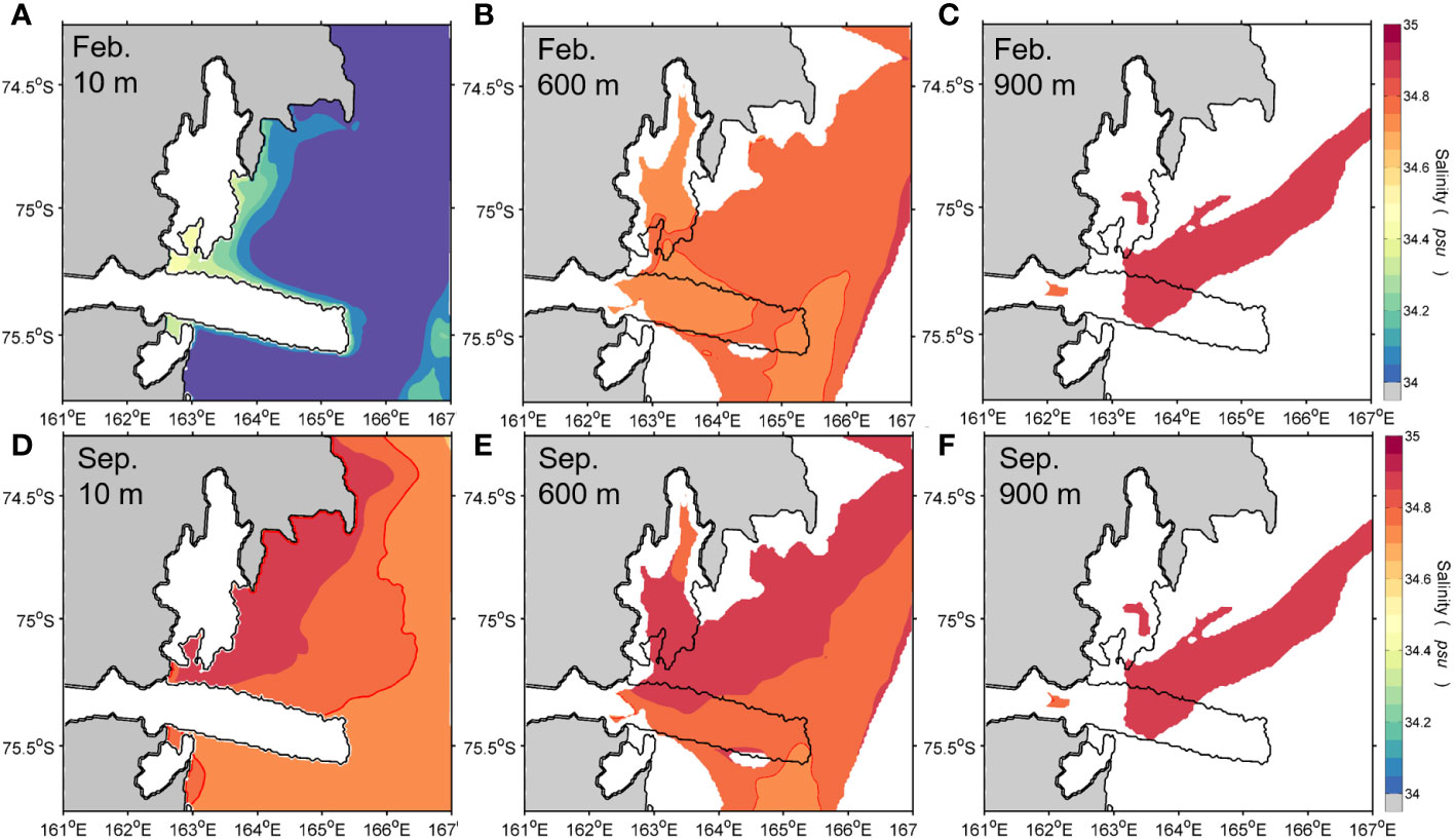
Figure 2 Horizontal distributions of salinity at (A, D) 10 m, (B, E) 600 m, and (C, F) 900 m depths in February (upper) and September (lower panels) from the ocean model. Black line indicates the ice shelf boundary for NIS and DIT.

To better quantitatively describe the HSSW distribution, a tracer experiment is computed by inserting a passive tracer into the ocean model domain. A passive tracer is released at the surface layer where the surface salinity is higher than 34.8 due to active sea–ice production in TNBP to determine the contribution of HSSW formed by brine rejection at the surface. In other words, the passive tracer represents the dense shelf water formed by the polynya’s sea–ice production, which is not released during austral summer when the surface salinity is less than 34.8 due to sea–ice melting. As expected, no tracer is observed at the surface layer (10 m) in February, but its concentration gradually increases from the surface to the bottom layer (Figures 3A–C). The tracer representing the HSSW is distributed over the DB (more than 80% of the concentration at 900 m), indicating that the HSSW formed during the previous winter is consistently distributed on the bottom layer throughout the year. Unlike the austral summer, a high concentration of the tracer is distributed along the northern margin of the DIT and the western shore of TNB at the surface in September, similar to that of an L-shaped polynya in the TNB (Figures 3D, S7D). Because the density of water increases with salinity and surface water freezing is accompanied by brine rejection, the thus-formed near-surface water tends to sink. Therefore, the tracer concentration of more than 90% is dominant in the lower layers of the water column in the TNB, consistent with the salinity pattern (Figures 2, 3). These tracer distributions strongly support the HSSW formation through brine rejection from winter polynya sea–ice formation and the resultant deep convection revealed by the salinity distribution. In addition, the tracer enters the NIS cavity and flows along the seafloor to the grounding line, showing more than 90% of the tracer concentration that gradually decreased from the ice front to the grounding line (Figures 3, 4). These modeling results with the passive tracer experiment demonstrate the seasonal variability of HSSW formation in the TNB.

FIGURE 3

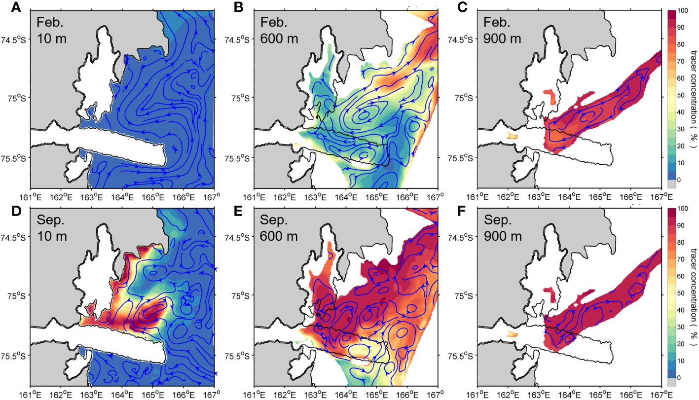
Figure 3 Same as in Figure 2, but for tracer concentration (%). Streamline is also shown by blue arrow lines.

FIGURE 4

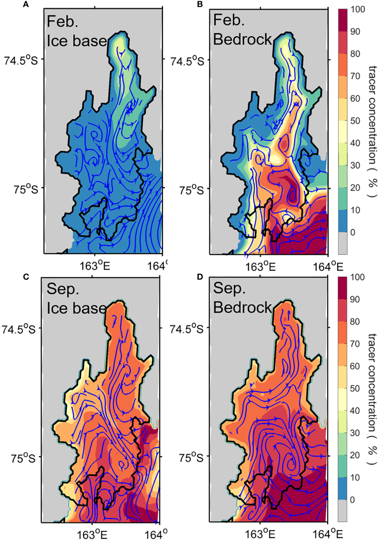
Figure 4 Horizontal distributions of tracer concentration and streamline along the (A, C) ice base and (B, D) bedrock of NIS in February (upper) and September (lower) from the ocean model. The ice shelf boundary is shown by black line.

4 Basal melting beneath the NIS

4.1 Seasonal evolution of the basal melt rates

The seasonal changes in water properties and associated ocean circulation can influence ocean–ice shelf interactions and consequent basal melt rates. Thus, changes in basal melting at the ice shelf base are examined to clarify the oceanic influence on the seasonal variability of the NIS basal melt (Figure 5). The simulated annual mean rate of basal melting over the entire NIS is $1.13\text{m}/\text{yr}$, almost similar to the finding of $1.6\pm 1.1\text{m}/\text{yr}$ in a recent study (Adusumilli et al., 2020). Although the simulated melt rate is slightly lower than that of satellite-based estimates, its value is within the observational uncertainty; thus, the model result is reasonable. The basal melting rate shows a completely different spatial behavior in season over the NIS base. In February, a rapid melting underside of the ice shelf is found close to the ice shelf front, showing up to $~ 5\text{m}/\text{yr}$ of basal melting in a limited area of the southeastern flank of NIS. The basal melting for the shallow parts of the ice draft of 200 m contributes 78% of the total NIS melt rate in February. The basal melt rate decreases toward the NIS grounding line, showing a moderate rate of $~ 1\text{m}/\text{yr}$. Compared with the basal melt rates in February, the melt rates near the NIS front dramatically decrease to below $0.5\text{m}/\text{yr}$, whereas basal melting near the grounding line becomes stronger in September (Figure 5B). High basal melting rates appear near the grounding line along the deep bathymetric trough in the NIS cavity, contributing 38% of the total rates of NIS basal melting in winter. The seasonal evolution of basal melt rates is more evident from the basal melting latitude–time plot along the NIS, highlighting that basal melting beneath the NIS is highly variable both in space and time.

FIGURE 5

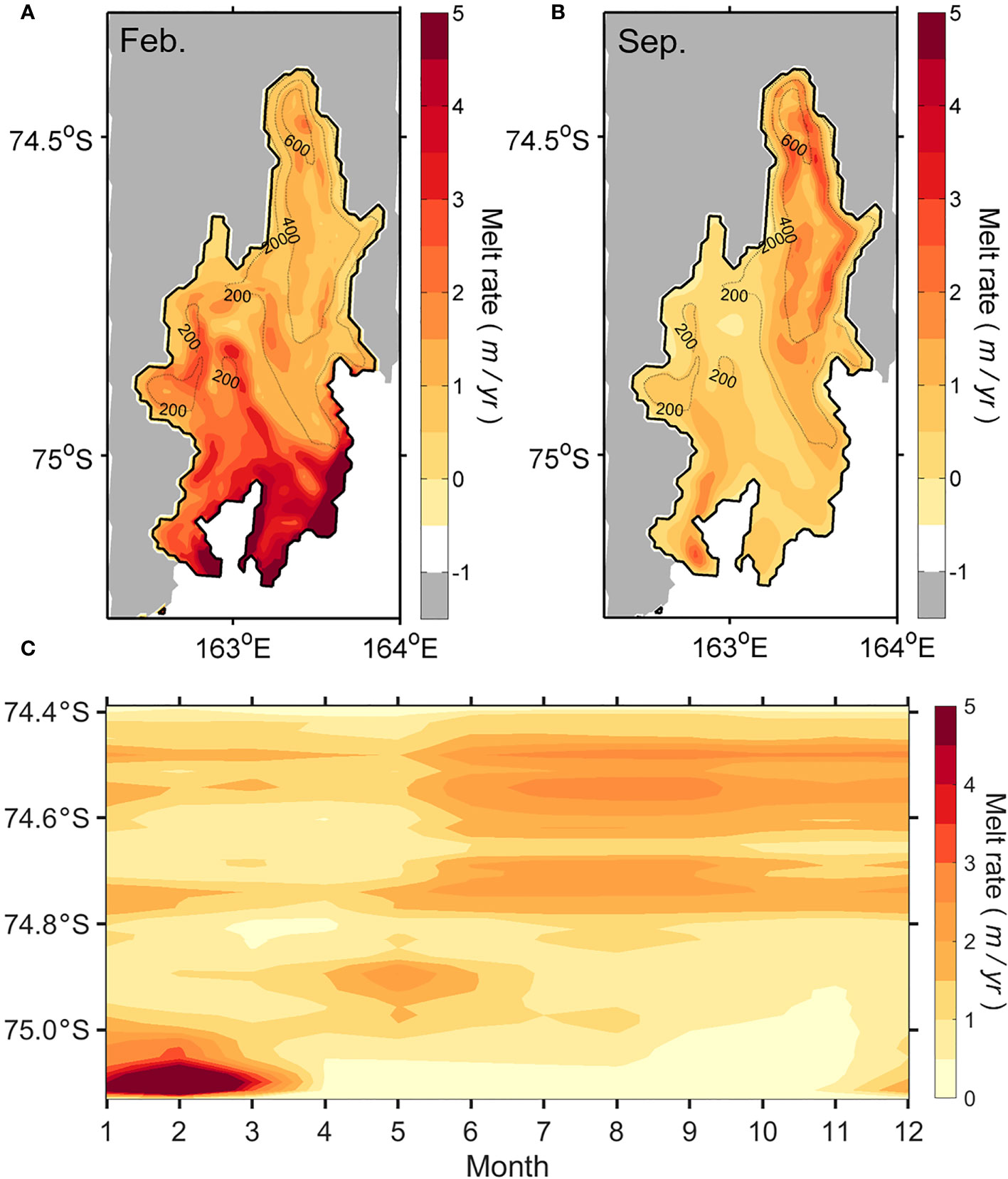
Figure 5 Rates of melting over the NIS estimated by the model. Horizontal distribution of melt rate in (A) February and (B) September. The bathymetry and the ice shelf boundary are shown by gray and black lines, respectively. (C) Time-latitude diagram of melt rate along the red line of NIS marked in Figure 1B.

4.2 Ocean-driven basal melt rates

The ice shelf basal melting rate is primarily driven by ocean heat transport entering the sub-ice cavity by the intrusion of warm surface waters, relatively warm CDW, or highly saline waters beneath ice shelves (Jacobs et al., 1992; Silvano et al., 2016; Stewart et al., 2019). Thus, the seasonal variation of basal melting depends on how ocean heat can be transported to the ice–ocean interface. The vertical sections of temperature and salinity along the NIS show the access of relatively warm and fresh surface water ($>-1.4°\text{C}$, $<34.5$) at the shallow portions of the NIS where the ice draft is less than about 400 m in February (Figures 6A, C). The upper layer is well stratified due to warm water transport to the ice shelf cavity at shallow depths. This warm water flows into the upper part of the NIS cavity through the southeastern flank of the NIS front from the southwestern TNB where polynyas absorb solar heat rapidly during summer. As the warm surface water moves under the ice shelf, ocean heat is transported into the ice shelf base in the upper part of the cavity, resulting in rapid basal melting at the ice shelf shallower than 400 m near the NIS front (Figure 5A). Due to active ice melting driven by the heat transmitted from the ocean to the ice shelf base, water at the ice base is relatively cooler and fresher than that in the upper part of the cavity. These results suggest that melting at the shallow-draft outer portions of the ice shelf is the dominant source of NIS basal mass loss during austral summer (dominated by Mode 3 melting). Meanwhile, the HSSW flows clockwise into the cavity along the NIS base, and some portions reach near the grounding line but with mostly limited access to the groundling line (Figures 4B, 6E). The tracer concentration of more than 50% is limited to the shallow-draft outer region of NIS at depths greater than 800 m, and the concentration decreases toward the grounding line along the sea floor. These results indicate that during austral summer, relatively warm surface water from the southwestern TNB drives high basal melting rates near the NIS front. On the other hand, the HSSW access to the grounding line is restricted, causing low basal melting rates near the grounding line.

FIGURE 6

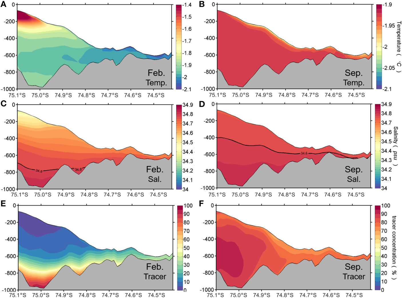
Figure 6 Vertical sections of (A, B) temperature, (C, D) salinity, and (E, F) tracer concentration along the red line of NIS marked in Figure 1B in February (left) and September (right panels) from the ocean model. Black contour line in (B, C) indicates a value of 34.8 psu.

Unlike in summer, relatively saline water fills most of the water column in the cavity beneath the NIS and has access to the grounding line in September when the polynya processes are strong enough to produce HSSW (Figure 6). The HSSW in the TNBP is widespread and enters the NIS cavity along the western NIS basal slope from the south and flows towards the grounding line along the sea floor (Figure 4D). Because of the seawater freezing point’s dependence on pressure and salinity, the water accessing the ocean cavity is warmer than the in-situ freezing point and thus melts the underside of the NIS, producing supercooled waters relative to the freezing point at shallower depths along the ice shelf base (Figure 6B). A high concentration of the tracer (>70%) fills the entire water column in the NIS cavity except along the ice shelf base (Figure 6F). The HSSW flowing into the cavity spreads along the seafloor to reach the area near the grounding line, where the tracer concentration reaches about 70% (Figure 4D). The HSSW intrusion to the grounding line drives high basal melting rates there and produces ISW by mixing with meltwater, therefore showing a relatively low concentration of the tracer along the ice shelf base. The HSSW formed in the TNBP during austral winter reaches the deeper part of the NIS cavity and drives more basal melting along the ice shelf base from greater depths, consistent with the “Mode 1” melting process (Jacobs et al., 1992).

Diagnostic analysis of temperature change rate (Text S4) further demonstrates that the summer melting near the NIS front is dominated by advection processes, whereas diffusion processes contribute more to basal melting near the grounding line in winter (Figure S8). In warm season, the increase in the local rate of temperature changes occurs at the shallow draft outer portions of the NIS (Figure S8A). The total advection term dominates the changes in temperature, which might be attributed to the relatively warm surface water in TNB during summer. On the other hand, the contribution of diffusion process shows an abrupt increase at the deeper parts of the NIS in cold season, providing support to the “Mode 1” melting process (Figure S8D).

5 Contribution of tides and realistic cavity geometry

Tides are known to affect sea–ice production and basal melting under ice shelves (e.g., Jourdain et al., 2019; Hausmann et al., 2020). In addition, the spatial distribution of basal melting is very sensitive to model geometry as well as tides (Mueller et al., 2012). Because the ocean underneath the ice shelves is completely isolated from the atmosphere by thick ice, tides instead of winds become a major source of oceanic kinetic energy for conversion to mixing in the ice shelf cavities. The tidal currents in the cavity interact with the topographies of the ice base and bedrock, inducing turbulent mixing. The tide-induced turbulent mixing within the ice shelf cavity affects basal melting by changing the heat and salt exchange through the ice shelf-ocean boundary layer. In this section, impacts of tides and cavity geometry on the NIS basal melting are estimated by conducting two additional experiments; one is without tides, and the other one uses original RTopo2 (Figure 7). A comparison of the sensitivity experiments with the control simulation exhibits a significant difference during summer but a small one during winter (Figure S9). Because the water is completely mixed from surface to bottom and the very cold-salty water occupies the whole water column during most of the cold season. Thus, we focus on the impact of tides and realistic cavity geometry on the basal melting beneath the NIS during the warm season when thermohaline stratification occurs in the TNB.

FIGURE 7

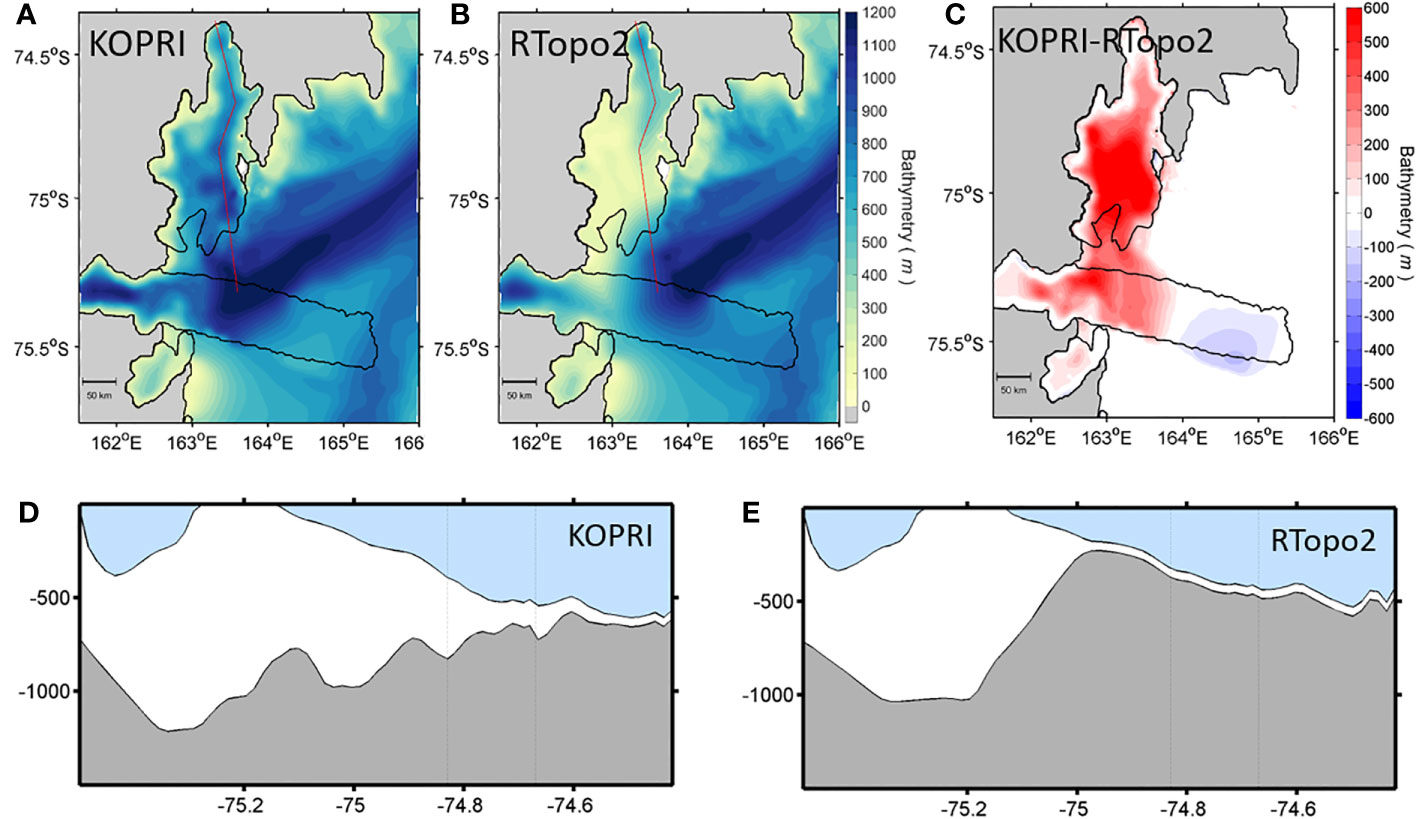
Figure 7 Model bathymetry estimated by (A) airborne gravity surveys provided from KOPRI and (B) original RTopo2 data. (C) Horizontal difference between two model bathymetries (A minus B). (D, E) The floating ice surface and base, and depth of the sea floor along the red line marked in (A, B).

Tides increase the basal melting of the shallow-draft outer portions of the ice shelf in February (austral summer), particularly those shallower than 200 m, making up a substantial increase of 30% relative to the result without tides (Figure 8A). This is similar to the modeling result for the Ross Ice Shelf reported by Arzeno et al. (2014). Tidal currents in high latitude oceans tend to be quite barotropic because of the weak stratification (MacAyeal, 1984; Robertson et al., 1998). Here the spatial variability of monthly barotropic currents is characterized by using the time- and depth-averaged tidal current speed (Figure 9). Comparing the results with and without tides demonstrates that tides drive strong barotropic currents in the cavity and a robust thermal exchange at the ocean-ice interface. The strong barotropic current speed appears on the shallow ice draft region, particularly along the sloping ice shelf base (Figure 9B), which induces turbulent mixing by interaction with the ice shelf topography. This facilitates the heat exchange between the ocean and ice shelf (Figure 9E), resulting in substantial basal melting. The increased basal melting in areas of shallow ice draft in the upper part of the cavity, particularly near the ice front, can be also linked to an enhanced heat absorption within the TNBP, which can be induced by reduced sea–ice production due to tidal forcing. Koentopp et al. (2005) investigated the effects of tides on the seasonal fluctuations of the sea-ice cover using a sea-ice model and showed a decrease in sea-ice concentration when including tidal forcing into the model. They found that during summer enhanced absorption of radiation and additional entrainment of warmer waters into the mixed layer by tidal current are responsible for this reduction. During austral summer when significant open water exists, including the coastal TNBP, the tidal effects lead to smaller minimum sea-ice extent than those without tides and thus increased solar absorption in the surface layer, driving rapid surface heating in TNBP (Figure 8B). Consequently, the simulation with tides exhibits enhanced solar heating of the surface water and the subsequent intrusion of this relatively warm water into the upper part of the NIS cavity where the ice draft is lower than 400 m (Figure 8C). The experiment without tides further suggests that the inflow of solar-heated surface waters from the adjacent TNBP is important in driving NIS basal melting during summer.

FIGURE 8

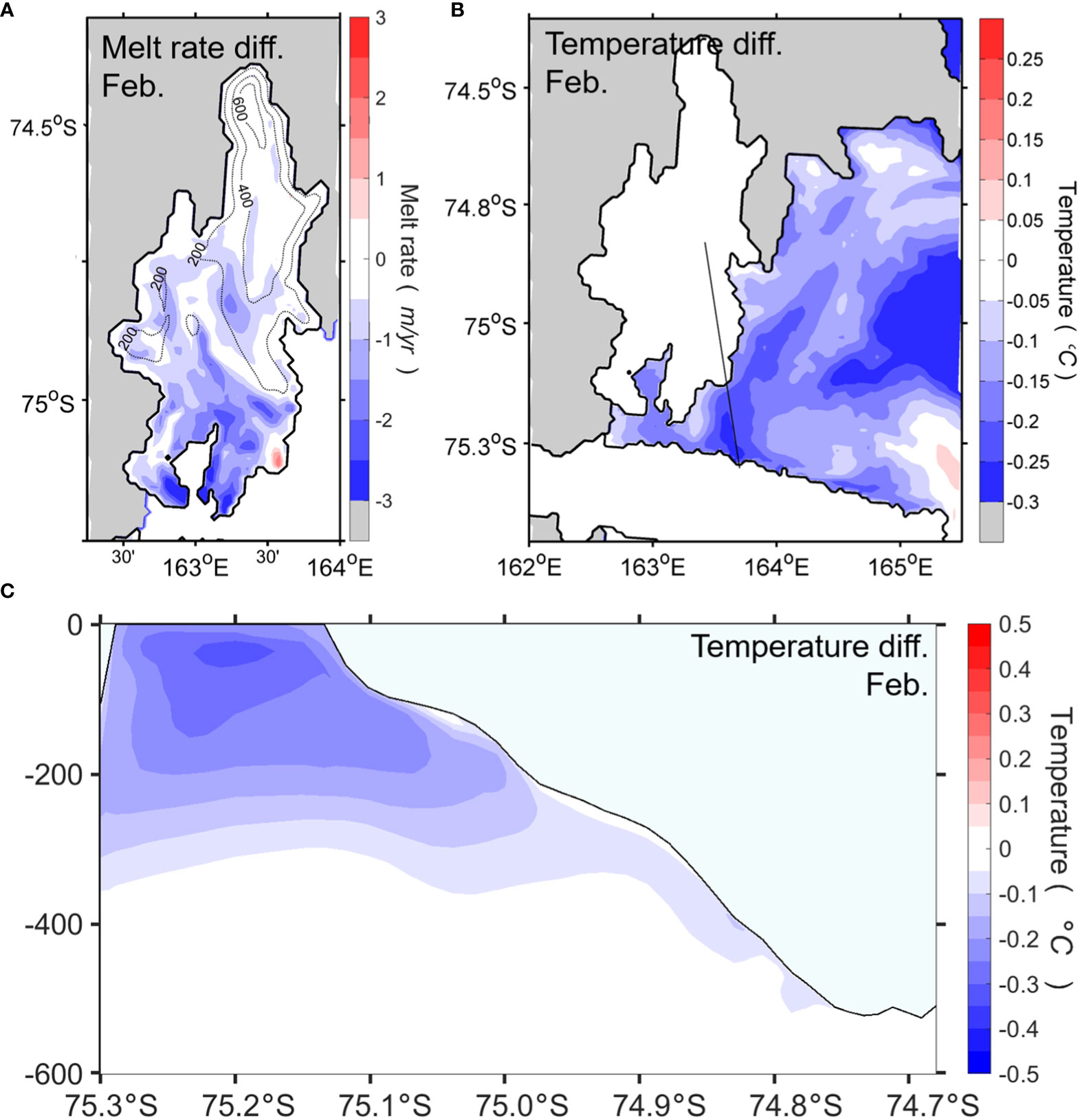
Figure 8 Differences between the model results with and without tides in February. (A) Difference in melt rate along the base of NIS. The bathymetry and the ice shelf boundary are shown by gray and black lines, respectively. (B) Difference in temperature at ocean surface layer. (C) Difference in temperature along the vertical section of black line marked in (B). Negative values indicate higher in the simulation with tides.

FIGURE 9

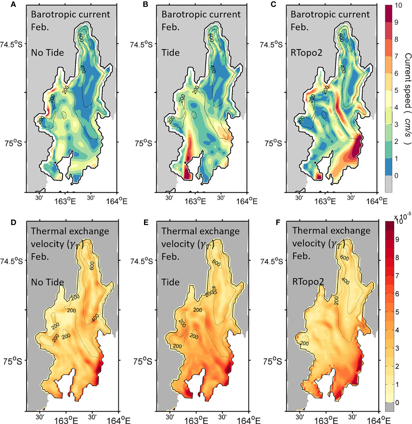
Figure 9 Horizontal distributions of barotropic current speed (upper) and thermal exchange velocity (lower) in February from the sensitivity experiments (A, D) without tides using realistic cavity geometry, (B, E) with tides using realistic cavity geometry, and (C, F) with tides using original RTopo2, respectively. The ice shelf boundary is shown by black line.

The sensitivity result using cavity geometry estimated by original RTopo2 reveals an excessive basal melting just near the NIS frontal band (Figure 10A). Strong time-averaged barotropic currents and hence an enhanced turbulent exchange rate for heat are restricted in a narrow frontal band of NIS (Figures 9C, F), corresponding to the excessive melting region (Figure 10A). RTopo2 bathymetry shows seafloor hill-like topography at the entrance of the NIS cavity (Figures 7E, 10C). This topographic feature induces abrupt changes in water column thickness and strong tide-topography interaction at the ice shelf front (Figure 9C). Consequently, locally enhanced tide-induced vertical mixing occurs under the NIS calving front due to interaction with the unrealistic topography (Figure 9F), which is responsible for warmer/cooler water at/above the depth of the sill. Namely, the surface layer becomes cooler due to substantial basal melting around the NIS calving front while the water at the depth of the sill becomes warmer due to mixing through tide-topography interaction (Figures 10B, C).

FIGURE 10

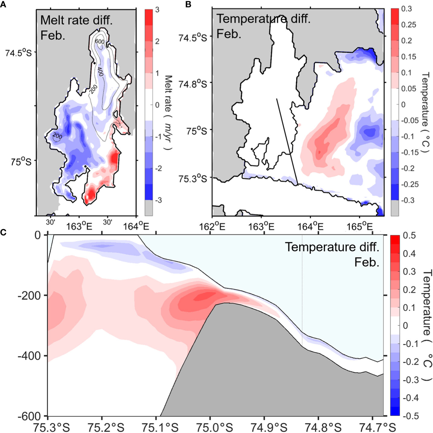
Figure 10 Same as in Figure 8, but for model results using realistic cavity geometry and original RTopo2 bathymetry. Negative values indicate higher in the simulation using realistic cavity geometry.

6 Summary

Using a regional coupled sea-ice/ocean circulation model including the ocean–ice shelf dynamics/thermodynamics, a numerical simulation with tides and realistic cavity geometry is conducted on the NIS in the TNB, East Antarctica, to explore ocean-driven basal melting of a cold-water cavity ice shelf. The results highlight the seasonal spatiotemporal variability in melt rates from different modes of basal melting occurring at different depths of the NIS base. During austral summer, the basal melt rate near the grounding line is moderate (for ice draft deeper than 400 m), whereas that for shallow-draft outer regions of the NIS increases toward the ice shelf front, contributing 78% of the total NIS melting rate. The enhanced melting near the ice shelf front is dominated by Mode 3 processes. Solar-heated surface waters advect under the ice shelf and drive strong melting in shallower ice drafts along the ice shelf front, suggesting that melting at the shallow ice shelf base is the dominant source of the NIS basal mass loss during austral summer. Meanwhile, during austral winter, the basal melt rate near the ice front dramatically decreases, whereas basal melting near the grounding line increases much above summer values. The increased basal melt rates near the grounding line are closely linked to the active formation of HSSW in the TNBP during austral winter, which is characterized by Mode 1 melting processes. The intrusion of HSSW produced by active TNBP that flows into the cavity beneath NIS toward the deep grounding line explains 36% of the total melting rate of NIS in winter.

To identify the contribution of tides and realistic cavity geometry to basal melt rates of the NIS, two sensitivity experiments are performed using the same initial and boundary conditions as in the control simulation: one is without tides, and the other one uses original RTopo2. The additional experiments demonstrate that basal melting is very sensitive to tide and cavity geometry. Tidal effects increase the melting of NIS, particularly contributing as much as 30% to the shallow ice draft region along the sloping ice shelf base. Tides induce turbulent mixing by interacting with topographies of ice base and bedrock, stimulating the exchange of heat and salt between the ocean and ice shelf. Sea-ice production is also reduced due to tides, leading to surface heating in TNBP during summer. In addition, basal melt rates beneath the NIS responded directly to the cavity geometry. Spurious vertical mixing is locally induced and enhanced by interaction between tides and the unrealistic topography, resulting in excessive basal melting near the NIS frontal band where a sill is featured in original RTopo2. The sensitivity experiments have shown that tides and realistic cavity geometry bring a significant improvement in the estimation of basal melt rates through a numerical model.

Our results suggest that accurately modeling ocean-driven melting beneath ice shelves is crucial to predicting their temporal and spatial mass loss. Seasonal variability signatures for different ocean-driven melting modes also have implications for the regional basal mass balance around the ice shelves. As heat absorption and HSSW formation are driven by atmospheric processes in polynya, ice shelf melting is likely to vary with atmospheric conditions and is associated with ocean circulations on interannual and longer time scales. As sea–ice concentration decreases because of ocean warming, ice shelves change with thinning ice fronts and grounding line retreat by the ocean and so are more vulnerable to a warming climate system. The potential for climate-related ice shelf melting provides motivations for further studies, including observational and modeling efforts focused on ocean–ice shelf interactions and longer-term effects on basal melting beneath ice shelves.

Data availability statement

The original contributions presented in the study are included in the article/Supplementary Material, further inquiries can be directed to the corresponding author.

Author contributions

TK, EKJ, and J-HM contributed to the conception and design of the study. J-SH performed the numerical experiments and produced all Figures. TK, J-HM, and J-SH contributed to the data processing and analysis. S-KS and WSL contributed to scientific discussion. EKJ and WSL provided the study materials. The paper was written by TK and J-HM with input from all authors. All authors contributed to the article and approved the submitted version.

Funding

This work was supported by the National Research Foundation of Korea (NRF) grant funded by the Korea government (Ministry of Science and ICT) (NRF-2023R1A2C1006812) and Basic Science Research Program through the NRF funded by the Ministry of Education, Korea (NRF-2021R1I1A2050261). S-KS is supported by Basic Science Research Program through the NRF funded by the Ministry of Science, ICT and Future Planning (2020R1A2C2011081), and EKJ and WSL are supported by Korea Institute of Marine Science & Technology Promotion (KIMST) funded by the Ministry of Oceans and Fisheries (RS-2023-00256677; PM23020).

Conflict of interest

The authors declare that the research was conducted in the absence of any commercial or financial relationships that could be construed as a potential conflict of interest.

Publisher’s note

All claims expressed in this article are solely those of the authors and do not necessarily represent those of their affiliated organizations, or those of the publisher, the editors and the reviewers. Any product that may be evaluated in this article, or claim that may be made by its manufacturer, is not guaranteed or endorsed by the publisher.

Supplementary material

The Supplementary Material for this article can be found online at: https://www.frontiersin.org/articles/10.3389/fmars.2023.1249562/full#supplementary-material

References

Adusumilli S., Fricker H. A., Medley B., Padman L., Siegfried M. R. (2020). Interannual variations in meltwater input to the Southern Ocean from Antarctic ice shelves. Nat. Geosci. 13, 616–620. doi: 10.1038/s41561-020-0616-z

PubMed Abstract | CrossRef Full Text | Google Scholar

Aoki S., Takahashi T., Yamazaki K., Hirano D., Ono K., Kusahara K., et al. (2022). Warm surface waters increase Antarctic ice shelf melt and delay dense water formation. Commun. Earth Environ. 3, 142. doi: 10.1038/s43247-022-00456-z

CrossRef Full Text | Google Scholar

Arzeno I. B., Beardsley R. C., Limeburner R., Owens B., Padman L., Springer S. R., et al. (2014). Ocean variability contributing to basal melt rate near the ice front of Ross Ice Shelf, Antarctica. J. Geophys. Res.: Oceans 119, 4214–4233. doi: 10.1002/2014JC009792

CrossRef Full Text | Google Scholar

Budgell W. P. (2005). Numerical simulation of ice-ocean variability in the Barents Sea region: towards dynamical downscaling. Ocean Dyn. 55, 370–387. doi: 10.1007/s10236-005-0008-3

CrossRef Full Text | Google Scholar

Buffoni G., Cappelletti A., Picco P. (2002). An investigation of thermohaline circulation in the Terra Nova Bay polynya. Antarct. Sci. 14, 83–92. doi: 10.1017/S0954102002000615

CrossRef Full Text | Google Scholar

Depoorter M. A., Bamber J. L., Griggs J. A., Lenaerts J. T. M., Ligtenberg S. R. M., van den Broeke M. R., et al. (2013). Calving fluxes and basal melt rates of Antarctic ice shelves. Nature 502, 89–92. doi: 10.1038/nature12567

PubMed Abstract | CrossRef Full Text | Google Scholar

Ding Y., Cheng X., Li X., Shokr M., Yuan J., Yang Q., et al. (2020). Specific relationship between the surface air temperature and the area of the Terra Nova Bay Polynya, Antarctica. Adv. Atmos. Sci. 37, 532–544. doi: 10.1007/s00376-020-9146-2

CrossRef Full Text | Google Scholar

Dinniman M. S., Klinck J. M., Smith W. O. (2007). Influence of sea ice cover and icebergs on circulation and water mass formation in a numerical circulation model of the Ross Sea, Antarctica. J. Geophys. Res. 112, C11013. doi: 10.1029/2006JC004036

CrossRef Full Text | Google Scholar

Dinniman M. S., Klinck J. M., Smith W. O. Jr. (2011). A model study of Circumpolar Deep Water on the West Antarctic Peninsula and Ross Sea continental shelves. Deep Sea Res. Part II Top. Stud. Oceanogr. 58, 1508–1523. doi: 10.1016/j.dsr2.2010.11.013

CrossRef Full Text | Google Scholar

Dutrieux P., De Rydt J., Jenkins A., Holland P. R., Ha H. K., Lee S. H., et al. (2014). Strong sensitivity of pine island ice-shelf melting to climatic variability. Science 343, 174–178. doi: 10.1126/science.1244341

PubMed Abstract | CrossRef Full Text | Google Scholar

Dziak R.P., Lee W.S., Haxel J.H., Matsumoto H., Tepp G., Lau T.–K., et al. (2019). Hydroacoustic, meteorologic and seismic observations of the 2016 Nansen ice shelf calving event and iceberg formation. Front. Earth Sci. 7, 183. doi: 10.3389/feart.2019.00183

CrossRef Full Text | Google Scholar

Egbert G. D., Erofeeva S. Y. (2002). Efficient inverse modeling of barotropic ocean tides. J. Atmos. Ocean. Technol. 19, 183–204. doi: 10.1175/1520-0426(2002)019<0183:EIMOBO>2.0.CO;2

CrossRef Full Text | Google Scholar

Fairall C. W., Bradley E. F., Hare J. E., Grachev A. A., Edson J. B. (2003). Bulk parameterization of air–sea fluxes: Updates and verification for the COARE algorithm. J. Clim. 16, 571–591. doi: 10.1175/1520-0442(2003)016<0571:BPOASF>2.0.CO;2

CrossRef Full Text | Google Scholar

Fusco G., Budillon G., Spezie G. (2009). Surface heat fluxes and thermohaline variability in the Ross Sea and in Terra Nova Bay polynya. Cont. Shelf Res. 29, 1887–1895. doi: 10.1016/j.csr.2009.07.006

CrossRef Full Text | Google Scholar

Gwyther D. E., Spain E. A., King P., Guihen D., Williams G. D., Evans E., et al. (2020). Cold ocean cavity and weak basal melting of the Sørsdal ice shelf revealed by surveys using autonomous platforms. J. Geophys. Res. Oceans 125, e2019JC015882. doi: 10.1029/2019JC015882

CrossRef Full Text | Google Scholar

Haidvogel D. B., Arango H., Budgell W.P., Cornuelle B.D., Curchitser E., Di Lorenzo E., et al. (2008). Ocean forecasting in terrain-following coordinates: Formulation and skill assessment of the Regional Ocean Modeling System. J. Comput. Phys. 227, 3595–3624. doi: 10.1016/j.jcp.2007.06.016

CrossRef Full Text | Google Scholar

Hausmann U., Sallée J. B., Jourdain N., Mathiot P., Rousset C., Madec G., et al. (2020). The role of tides in ocean–ice-shelf interactions in the southwestern Weddell Sea. J. Geophys. Res.-Oceans 125, e2019JC015847. doi: 10.1029/2019JC015847

CrossRef Full Text | Google Scholar

Hedstrom K. (2016). Technical manual for a coupled sea-ice/ocean circulation model (Version 4) (Alaska OCS Region: U.S. Dept. of the Interior, Bureau of Ocean Energy Management), 176.

Google Scholar

Hellmer H. H., Olbers D. J. (1989). A two- dimensional model for the thermohaline circulation under an ice shelf. Antarct. Sci. 1, 325–336. doi: 10.1017/S0954102089000490

CrossRef Full Text | Google Scholar

Hersbach H., Bell B., Berrisford P., Hirahara S., Horányi A, Muñoz-Sabater J., et al. (2020). The ERA5 global reanalysis. Q. J. R. Meteorol. Soc 146, 1999–2049. doi: 10.1002/qj.3803

CrossRef Full Text | Google Scholar

Holland D. M., Jenkins A. (1999). Modeling thermodynamic ice-ocean interactions at the base of an ice shelf. J. Phys. Oceanogr. 29, 1787–1800. doi: 10.1175/1520-0485(1999)029<1787:MTIOIA>2.0.CO;2

CrossRef Full Text | Google Scholar

Holland D. M., Nicholls K. W., Basinski A. (2020). The Southern Ocean and its interaction with the Antarctic Ice Sheet. Science 367, 1326–1330. doi: 10.1126/science.aaz5491

PubMed Abstract | CrossRef Full Text | Google Scholar

Jacobs S. S., Giulivi C. F. (1985). Interannual ocean and sea ice variability in the Ross Sea. Ocean Ice Atmosphere: Interact. at Antarctic Continental Margin 75, 135–150. doi: 10.1029/ar075p0135

CrossRef Full Text | Google Scholar

Jacobs S. S., Hellmer H. H., Doake C. S. M., Jenkins A., Frolich R. M. (1992). Melting of ice shelves and the mass balance of Antarctica. J. Glaciol. 38, 375–387. doi: 10.3189/S0022143000002252

CrossRef Full Text | Google Scholar

Jacobs S. S., Hellmer H. H., Jenkins A. (1996). Antarctic ice sheet melting in the southeast Pacific. Geophys. Res. Lett. 23, 957–960. doi: 10.1029/96GL00723

CrossRef Full Text | Google Scholar

Jacobs S. S., Jenkins A., Giulivi C., Dutrieux P. (2011). Stronger ocean circulation and increased melting under Pine Island Glacier ice shelf. Nat. Geosci. 4, 519–523. doi: 10.1038/ngeo1188

CrossRef Full Text | Google Scholar

Jendersie S., Williams M. J. M., Langhorne P. J., Robertson R. (2018). The density-driven winter intensification of the Ross Sea circulation. J. Geophys. Res.-Oceans 123, 1–23. doi: 10.1029/2018JC013965

CrossRef Full Text | Google Scholar

Jenkins A., Shoosmith D., Dutrieux P., Jacobs S., Kim T. W., Lee S. H., et al. (2018). West Antarctic Ice Sheet retreat in the Amundsen Sea driven by decadal oceanic variability. Nat. Geosci. 11, 733–738. doi: 10.1038/s41561-018-0207-4

CrossRef Full Text | Google Scholar

Jourdain N. C., Molines J. M., Le Sommer J., Mathiot P., Chanut J., de Lavergne C., et al. (2019). Simulating or prescribing the influence of tides on the Amundsen Sea ice shelves. Ocean Model. 133, 44–55. doi: 10.1016/j.ocemod.2018.11.001

CrossRef Full Text | Google Scholar

Kim T., Jin E. K., Na J. S., Lee C. K., Lee W. S., Moon J.-H. (2022). Numerical simulation of ocean - ice shelf interaction: water mass circulation in the Terra Nova Bay, Antarctica. Ocean Polar Res. 30, 269–285. doi: 10.4217/OPR.2022027(in Korean with English abstract

CrossRef Full Text | Google Scholar

Koentopp M., Eisen O., Kottmeier C., Padman L., Lemke P. (2005). Influence of tides on sea ice in the Weddell Sea: investigations with a high-resolution dynamic-thermodynamic sea ice model. J. Geophys. Res. 110, C02014. doi: 10.1029/2004JC002405

CrossRef Full Text | Google Scholar

Lee W. S., Seo K.–W., Lee J., Kang Y., Lee H.–S., Dziak R.P., et al. (2019). Final report “Investigating Cryospheric Evolution of the Victoria Land, Antarctica” (Korea: Korea Polar Research Institute), 687. Available at: https://repository.kopri.re.kr/handle/201206/11131.

Google Scholar

Lellouche J.-M., Greiner E., Bourdallé Badie R., Garric G., Melet A., Drévillon M., et al. (2021). The copernicus global 1/12° Oceanic and sea ice GLORYS12 reanalysis. Front. Earth Sci. 9. doi: 10.3389/feart.2021.698876

CrossRef Full Text | Google Scholar

MacAyeal D. R. (1984). Thermohaline circulation below the Ross Ice Shelf: A consequence of tidally induced vertical mixing and basal melting. J. Geophys. Res. 89, 597–606. doi: 10.1029/JC089iC01p00597

CrossRef Full Text | Google Scholar

Marsland S. J., Church J. A., Bindoff N. L., Williams G. D. (2007). Antarctic coastal polynya response to climate change. J. Geophys. Res. 112, C07009. doi: 10.1029/2005JC003291

CrossRef Full Text | Google Scholar

Mellor G. L., Kantha L. (1989). An ice-ocean coupled model. J. Geophys. Res.-Oceans 94, 10937–10954. doi: 10.1029/JC094iC08p10937

CrossRef Full Text | Google Scholar

Millero F. J. (1978). Annex 6: Freezing point of seawater. Eighth report of the joint panel of oceanographic tables and standards. UNESCO Tech. Paper Mar. Sci. 28, 29–31.

Google Scholar

Mueller R. D., Padman L., Dinniman M. S., Erofeeva S. Y., Fricker H. A., King M. A. (2012). Impact of tide-topography interactions on basal melting of Larsen C Ice Shelf, Antarctica. J. Geophys. Res-Oceans 117, C05005. doi: 10.1029/2011JC007263

CrossRef Full Text | Google Scholar

Paolo F. S., Fricker H. A., Padman L. (2015). Volume loss from Antarctic ice shelves is accelerating. Science 348, 327–331. doi: 10.1126/science.aaa0940

PubMed Abstract | CrossRef Full Text | Google Scholar

Rignot E., Jacobs S., Mouginot J., Scheuchl B. (2013). Ice-shelf melting around Antarctica. Science 341, 266–270. doi: 10.1126/science.1235798

PubMed Abstract | CrossRef Full Text | Google Scholar

Rignot E., Mouginot J., Morlighem M., Seroussi H., Scheuchl B. (2014). Widespread, rapid grounding line retreat of Pine Island, Thwaites, Smith, and Kohler glaciers, West Antarctica, from 1992 to 2011. Geophys. Res. Lett. 41, 3502–3509. doi: 10.1002/2014GL060140

CrossRef Full Text | Google Scholar

Robertson R., Padman L., Egbert G. (1998). “Tides in the weddell sea,” in Oceanology of the Antarctic continental shelf. Antarct. Res. Ser., vol. 75 . Eds. Jacobs S., Weiss R. (Washington, D. C: AGU), 341–369.

Google Scholar

Rusciano E., Budillon G., Fusco G., Spezie G. (2013). Evidence of atmosphere–sea ice–ocean coupling in the Terra Nova Bay polynya (Ross Sea–Antarctica). Cont. Shelf Res. 61–62, 112–124. doi: 10.1016/j.csr.2013.04.002

CrossRef Full Text | Google Scholar

Sansiviero M., Maqueda M. A. M., Fusco G., Aulicino G., Flocco D., Budillon G. (2017). Modelling sea ice formation in the Terra Nova Bay polynya. J. Mar. Syst. 166, 4–25. doi: 10.1016/j.jmarsys.2016.06.013

CrossRef Full Text | Google Scholar

Schaffer J., Timmermann R., Arndt J. E., Kristensen S. S., Mayer C., Morlighem M., et al. (2016). A global, high-resolution data set of ice sheet topography, cavity geometry, and ocean bathymetry. Earth Syst. Sci. Data 8, 543–557. doi: 10.5194/essd-8-543-2016

CrossRef Full Text | Google Scholar

Semtner A. J. (1976). A model for the thermodynamic growth of sea ice in numerical investigations of climate. J. Phys. Oceanogr. 6, 379–389. doi: 10.1175/1520-0485(1976)006<0379:AMFTTG>2.0.CO;2

CrossRef Full Text | Google Scholar

Shchepetkin A. F., McWilliams J. C. (2005). The regional oceanic modeling system (ROMS): a split-explicit, free-surface, topography-following-coordinate oceanic model. Ocean Model. 9, 347–404. doi: 10.1016/j.ocemod.2004.08.002

CrossRef Full Text | Google Scholar

Silvano A., Rintoul S. R., Herraiz-Borreguero L. (2016). Ocean-ice shelf interaction in East Antarctica. Oceanography 29, 130–143. doi: 10.5670/oceanog.2016.105

CrossRef Full Text | Google Scholar

Stevens C., Lee W. S., Fusco G., Yun S., Grant B., Robinson N., et al. (2017). The influence of the Drygalski Ice Tongue on the local ocean. Ann. Glaciol. 58, 51–59. doi: 10.1017/aog.2017.4

CrossRef Full Text | Google Scholar

Stewart C. L., Christoffersen P., Nicholls K. W., Williams M. J. M., Dowdeswell J. A. (2019). Basal melting of Ross Ice Shelf from solar heat absorption in an ice-front polynya. Nat. Geosci. 12, 435–440. doi: 10.1038/s41561-019-0356-0

CrossRef Full Text | Google Scholar

Sturman A. P., Anderson M. R. (1986). On the sea-ice regime of the Ross Sea, Antarctica. J. Glaciol. 32, 54–59. doi: 10.1017/s0022143000006870

CrossRef Full Text | Google Scholar

Yoon S.-T., Lee W. S., Stevens C., Jendersie S., Nam S., Yun S., et al. (2020). Variability in high-salinity shelf water production in the Terra Nova Bay polynya, Antarctica. Ocean Sci. 16, 373–388. doi: 10.5194/os-16-373-2020

CrossRef Full Text | Google Scholar