ASTMEN: an adaptive spatiotemporal and multi-element fusion network for ocean surface currents forecasting

1 Introduction

Ocean surface currents refer to the continuous directional movement of surface water and have a great impact on human activities such as maritime route planning, marine environmental protection and marine fisheries. The huge kinetic energy carried by the surface currents is directly related to the fuel consumption of ships and the deployment of maritime pollution control (Chen et al., 2015; Van Sebille et al., 2020). Additionally, the heat carried by ocean surface currents affects the surrounding climate and the distribution of marine organisms, indirectly influencing the choice of fishing ground locations (Halpern et al., 2019; Peng et al., 2022). However, ocean surface currents, as part of the ocean system, are influenced by many factors such as sea surface height (SSH), sea surface temperature (SST) and sea surface salinity (SSS), resulting in complex spatiotemporal variations (Choi et al., 2021; Peng et al., 2022). Therefore, real-time and accurate continuous forecasting of ocean surface currents is a challenging task and holds significant importance.

For many years, numerical models such as Regional Ocean Modeling System (ROMS) (Shchepetkin and McWilliams, 2005), Hybrid Coordinate Ocean Model (HYCOM) (Bleck, 2002), Finite Volume Coastal Ocean Model (FVCOM) (Chen et al., 2006), Modular Ocean Model (MOM) (Griffies et al., 2005), and Princeton Ocean Model (POM) (Blumberg and Mellor, 1987) have been widely used for forecasting ocean currents. However, these models integrate various physical equations, including ocean dynamics and thermal salt transport equations. Consequently, these models necessitate intricate inputs, including boundary conditions and assimilation of diverse observations such as satellite data. And the computational demands are considerable, often relying on supercomputers (Lermusiaux, 2006; Rozier et al., 2007; Noori et al., 2017). As a result, these numerical models are difficult to implement and do not allow for real-time forecasting, which limits their applicability in many cases.

Rencently, data-driven models have become increasingly popular in marine and atmospheric environmental forecasting due to their ability to enable real-time forecasting, as well as being computationally efficient and easy to implement (Bolton and Zanna, 2019; Portillo Juan and Negro Valdecantos, 2022; Sun et al., 2023). Machine learning models such as linear regression (LR) (Sinha and Abernathey, 2021), random forest (RF) (Liu et al., 2023), genetic algorithms (GA) (Remya et al., 2012) and support vector regression (SVR) (Khosravi et al., 2018) are often used to solve time series forecasting problems, where the goal is to predict continuous numerical outputs by learning the relationship between input features and output targets. Nowadays, the most popular time series prediction methods are the ones based on deep learning, such as gated recurrent unit (GRU) (Song et al., 2020; Meng et al., 2021), LSTM (Graves and Graves, 2012; Bethel et al., 2022), and other recurrent neural networks (RNN). The basic structure of an RNN includes a recurrent unit, which takes as input not only the current time-step’s data but also the hidden state from the previous time-step. This design allows RNNs to incorporate past information into the current computation when processing sequential data, giving them the ability to remember. This memory characteristic enables RNNs to perform well in tasks such as natural language processing (NLP) and time series prediction (Elman, 1990; Medsker and Jain, 2001; Cao et al., 2023a).

However, the existing researches that apply deep learning methods to ocean currents forecasting tasks often focus more on the deep learning models themselves, neglecting the correlation between ocean currents and other marine elements, as well as the spatial dynamics of ocean currents. As a matter of fact, the movement of ocean currents is quite complicated, which is not only affected by ocean elements but also by topography, seasons, and other factors. The temporal variations of ocean currents are unstable, and their spatial patterns of motion are dynamically changing as well (Roemmich and Gilson, 2009; Chelton et al., 2011). Therefore, combining methods suitable for handling two-dimensional spatial information with RNN and integrating relevant ocean elements as auxiliary information has become a viable approach for spatiotemporal sequence prediction of ocean surface currents. Swin Transformer (Swin-T) (Liu et al., 2021) is an enhanced version of the Vision Transformer (VIT) model (Dosovitskiy et al., 2020), which introduces hierarchical self-attention mechanisms and window-based attention mechanisms on top of VIT to reduce the computational complexity of global attention (Vaswani et al., 2017; Li et al., 2022). This characteristic of Swin-T allows it to efficiently capture dependencies within the input data while reducing the computational burden of global attention. Consequently, Swin-T is well-suited to serve as a two-dimensional spatial information processing module in spatiotemporal forecasting models.

In this paper, a hybrid of improved Swin-T and LSTM neural network is developed to forecast ocean surface currents. Based on multi-element data at a given time, Swin-T models ocean currents at different scales from local to global through a shift window approach. This method achieves adaptive spatial information fusion for both different times in the same space and different spaces at the same time. It also improves the computational efficiency of self-attention, thereby expanding the spatial range and duration of ocean currents forecasting (Liu et al., 2021). In addition, we propose a weight selection module based on K-Nearest Neighbor (KNN) (Cover and Hart, 1967) to improve Swin-T (KSwin-T), which improves the accuracy and generalization of the model to capture the spatial structure of ocean currents. In this study, the spatiotemporal sequences generated by SST, SSS, SSH, eastward component of currents (U), and northward component of currents (V) are input into the LSTM for encoding and decoding. This allows for the extraction of interdependencies and synergistic changes among these elements to achieve accurate ocean currents forecasting.

In summary, our contributions are mainly in three aspects, as follows:

(1) We propose a hybrid Swin-T and LSTM model for spatiotemporal forecasting of ocean surface currents. The spatial information fusion module and the temporal feature extraction module together form a minimal network unit, which can adaptively capture the spatiotemporal correlation and interdependence between ocean surface currents and other related ocean elements at different spatiotemporal scales, achieving accurate and durable forecasts.

(2) We propose an improved Swin-T based on the idea of nearest neighbor (KNN). A weight selection module is designed to post-process the self-attention weight matrix in Swin-T, thereby retaining only the top K points with the highest weights for spatial information fusion. This improvement enables the model to obtain better generalization ability.

(3) This study presents a novel approach to developing deep learning-based models for predicting oceanic elements. We integrate specific physical characteristics of ocean currents to design methods, models, and experiments, enhancing both the model’s performance and development efficiency. Additionally, we employ oceanographic knowledge and visualization methods to explain the specific roles of each module in the deep learning model, thereby improving model interpretability.

2 Related work

The most common methods used in currents forecasting studies are numerical models which is based on physical processes and kinetic laws. Moore et al. constructed a 4-dimensional variational data assimilation system based on ROMS to forecast currents and analyzed the effect of multiple observations on the prediction results (Moore et al., 2011). Yu et al. analyzed the relationship between wind stress and surface currents based on HYCOM reanalysis data and proposed a method based on Ekman kinetics to predict warm currents in the South China Sea (Yu et al., 2022). However, the complex initial boundary conditions and the low forecasting efficiency of these methods present a challenge.

A few studies have also used machine learning methods, Kavousi-Fard et al. used SVR and Remya et al. used GA, but these studies are only adapted to specific regions and scenes which lack generalisation and are not suitable for spatiotemporal forecasting (Remya et al., 2012; Khosravi et al., 2018).

Recently, deep learning methods have been widely used in ocean currents forecasting. Immas et al. proposed two currents forecasting models, LSTM and Transformer, for real-time in-situ forecasting of currents at arbitrary locations (Immas et al., 2021). However, these models can only make single-point forecasts, which do not utilize spatial information around the sampling point and are not suitable for forecasting the whole region.

With the development of data assimilation techniques, ocean reanalysis data products are being improved and updated, and some deep learning-based studies also pay more attention to the spatiotemporal correlations of ocean currents. Thongniran et al. used convolutional neural networks (CNN) and GRU to construct a two-stage CNN-GRU model for spatial and temporal forecasting of ocean currents (Thongniran et al., 2019). Liu et al. used a single-stage ConvLSTM to fuse spatial information for ocean currents at any given moment, and the forecast accuracy is better than the two-stage approach (Liu et al., 2022). However, the fixed convolutional kernel in CNNs makes it difficult for these methods to address situations where different patterns of currents occur simultaneously and the patterns of currents change over time (Özturk et al., 2018; Gu et al., 2023). As a result, errors accumulate more quickly with persistent forecasting.

Self-attention is used in some studies for spatiotemporal forecasting of ocean currents. These methods can adaptively capture the spatiotemporal relationships of ocean currents, but lead to an increase in computational effort, thus reducing the spatial extent and duration of the forecasts (Li et al., 2022). Swin-T is a hierarchical self-attention method whose representation is computed with shifted windows. The shifted windows scheme brings greater efficiency by limiting self-attention computation to non-overlapping local windows, while also allowing cross-window connections. This approach has the flexibility to model at various scales which is well suited to complex ocean surface currents forecasting tasks (Liu et al., 2021).

LSTM has been widely adopted in the ocean domain and has achieved excellent performance in time-series prediction tasks (Meng et al., 2022). Additionally, many hybrid methods which add a spatial information fusion module to the LSTM are widely used for ocean elements forecasting (Jrges et al., 2021). Therefore, the hybrid method based on Swin-T and LSTM has great potential for spatiotemporal forecasting of ocean surface currents.

3 Study area, dataset and preprocessing

3.1 Study area and dataset

Figure 1 shows the study area of this paper, with a geographical range of 20°N-30°N and 120°E-130°E. This area is close to land and in the path of the Kuroshio, which is the most influential warm current in the world, resulting in significant fishing activity. The Kuroshio carries great kinetic energy and heat, which has a huge impact on the surrounding climate change and ocean currents, so it is of great importance to carry out research in this area (Chu, 1974; Warren, 1974; Hsin et al., 2008; Jin et al., 2010).

Figure 1

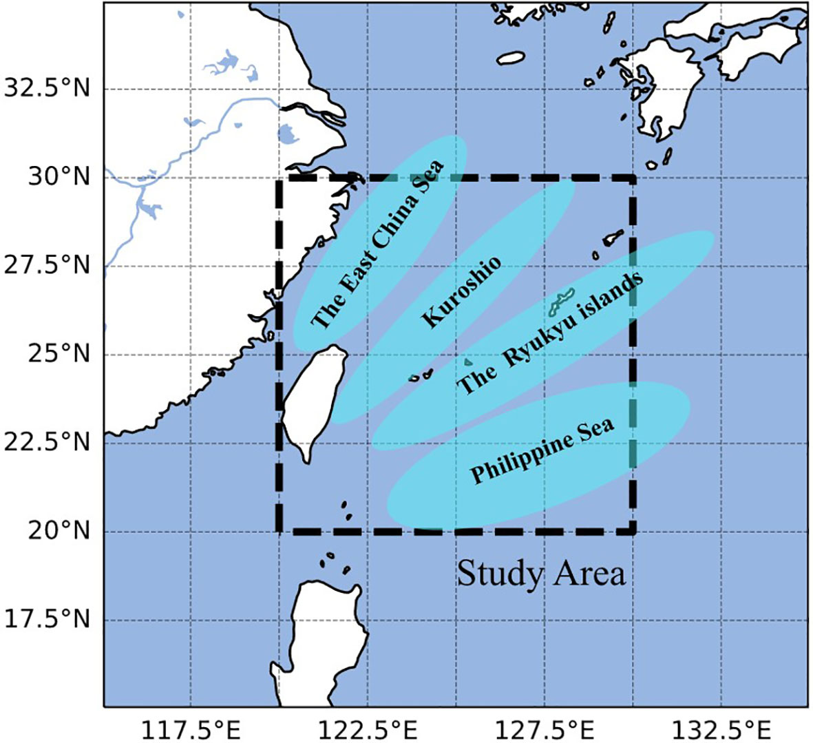
Figure 1 Geographical location information of study area.

This study uses the CORA2.0 reanalysis dataset from the National Marine Information Center(http://cora.nmdis.org.cn/). CORA2.0 includes five ocean elements, U, V, SST, SSS and SSH, of which U and V are the eastward and northward components of the ocean surface currents velocity, respectively. And the spatial resolution of the data is 0.1° × 0.1° with a time interval of one day, presented in daily average format.

Although CORA2.0 is a reanalysis dataset, there are still missing data in the land area. Therefore, data preprocessing was conducted in this study. Firstly, the missing data from the land areas were filled with zeros to reduce interference from the land areas during the prediction process. Subsequently, the ocean currents and other related ocean elements data were concatenated and max-min normalised in the feature dimension. Finally the original data were divided into time series samples according to time step T. Additionally, the data from 2015-01-01 to 2018-12-31 were used as the training set, and the data from 2019-01-01 to 2019-12-29 were used as the test set.

3.2 Data preprocessing

Part (a) of Figure 2 provides an overview of the data preprocessing operation, which consists of three main components:

(1) In the feature dimension, multiple ocean elements are concatenated, resulting in a data shape of (N,H,W,C), where N represents the total number of days of data, H and W represent the spatial dimensions, and C represents the number of features.

(2) Each feature of the data is normalized individually, and the data is scaled to a range of 0 to 1 to facilitate model training.

(3) The original data is divided into fixed-length time series based on the time step T. This results in a data shape of (M, T, H, W, C), where M represents the number of samples obtained after dividing the time series, and N = M × T.

Figure 2

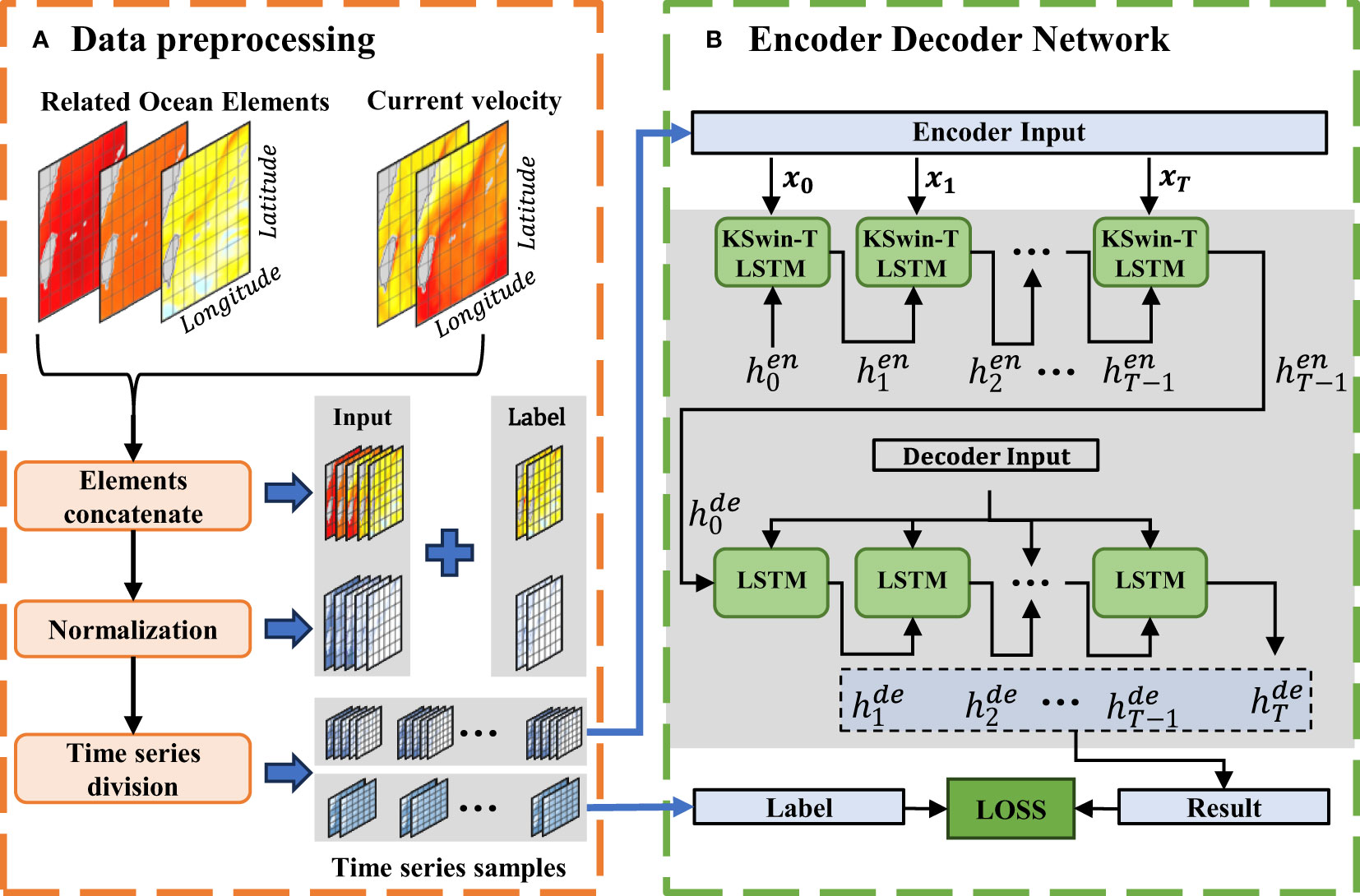
Figure 2 Framework of the proposed ASTMEN. (A) Preprocessing of relevant ocean elements data and ocean currents data. (B) Spatiotemporal forecasting model based on encoder-decoder networks.

4 Methods

4.1 The improved Swin-T based on KNN idea

In this study, KSwin-T was adopted as a spatial information fusion module for ocean currents. Swin-T is a hierarchical self-attention method whose representation is computed with shifted windows (Liu et al., 2021). As illustrated in Figure 3, Swin-T divides the input data into multiple non-overlapping sub-regions in layer k and shifts the position of the windows in the next layer, to achieve self-attention computation between different sub-regions. The shifted windows scheme limits the range of spatial information fusion, and this characteristic makes it particularly suitable for modeling complex and variable ocean surface currents at various scales.

Figure 3

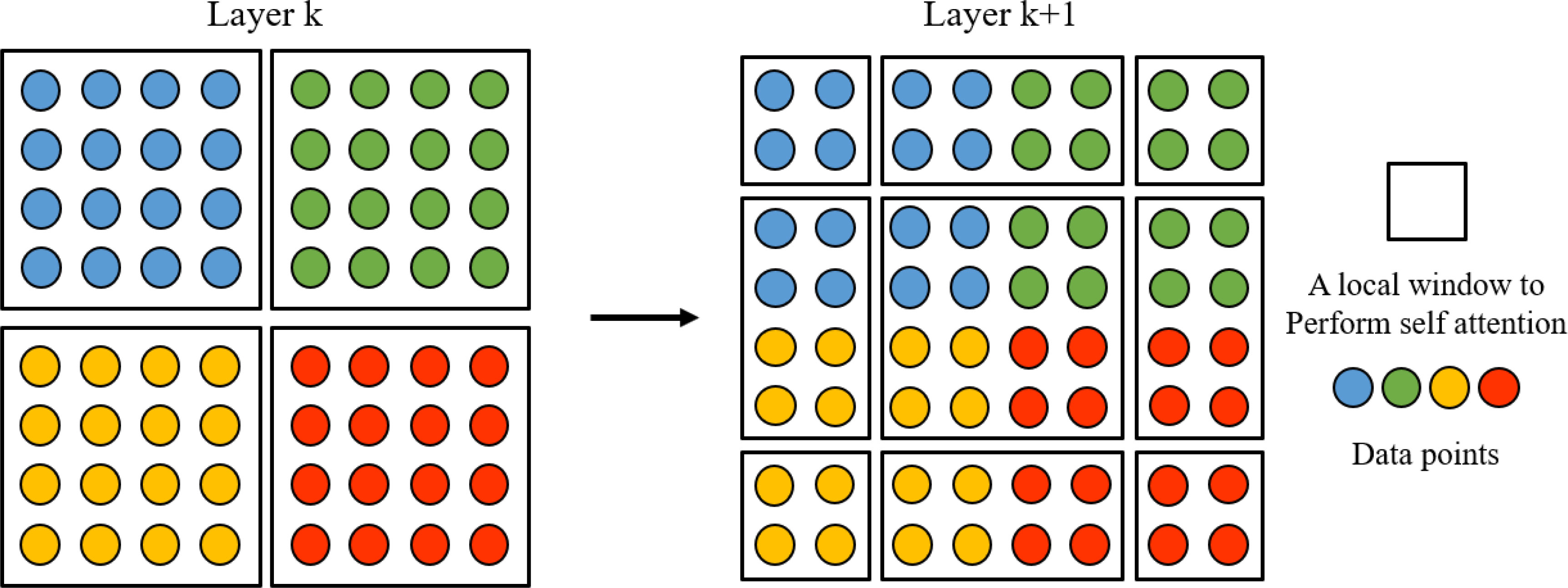
Figure 3 An illustration of the shifted window approach for computing spatial self-attention in Swin Transformer. In layer k (left), a regular window partitioning scheme is adopted, and self-attention is computed within each window. In the next layer k +1 (right), the window partitioning is shifted, resulting in new windows. The self-attention computation in the new windows crosses the boundaries of the previous windows in layer k, providing connections among them.

In order to identify the spatial structure of ocean currents more accurately, this study adopts the KNN idea to improve Swin-T. Specifically, we eliminate the interference of weakly correlated points by selecting only the top K neighboring points with the highest weights for spatial information fusion with the target point. As shown in Figure 4, D4 is used as the target point, and the weight matrix represents its attention weights with all points. When K is 5, KSwin-T selects the top 5 most relevant neighboring points B2, C3, B4, C4, and D4 for spatial information fusion.

Figure 4

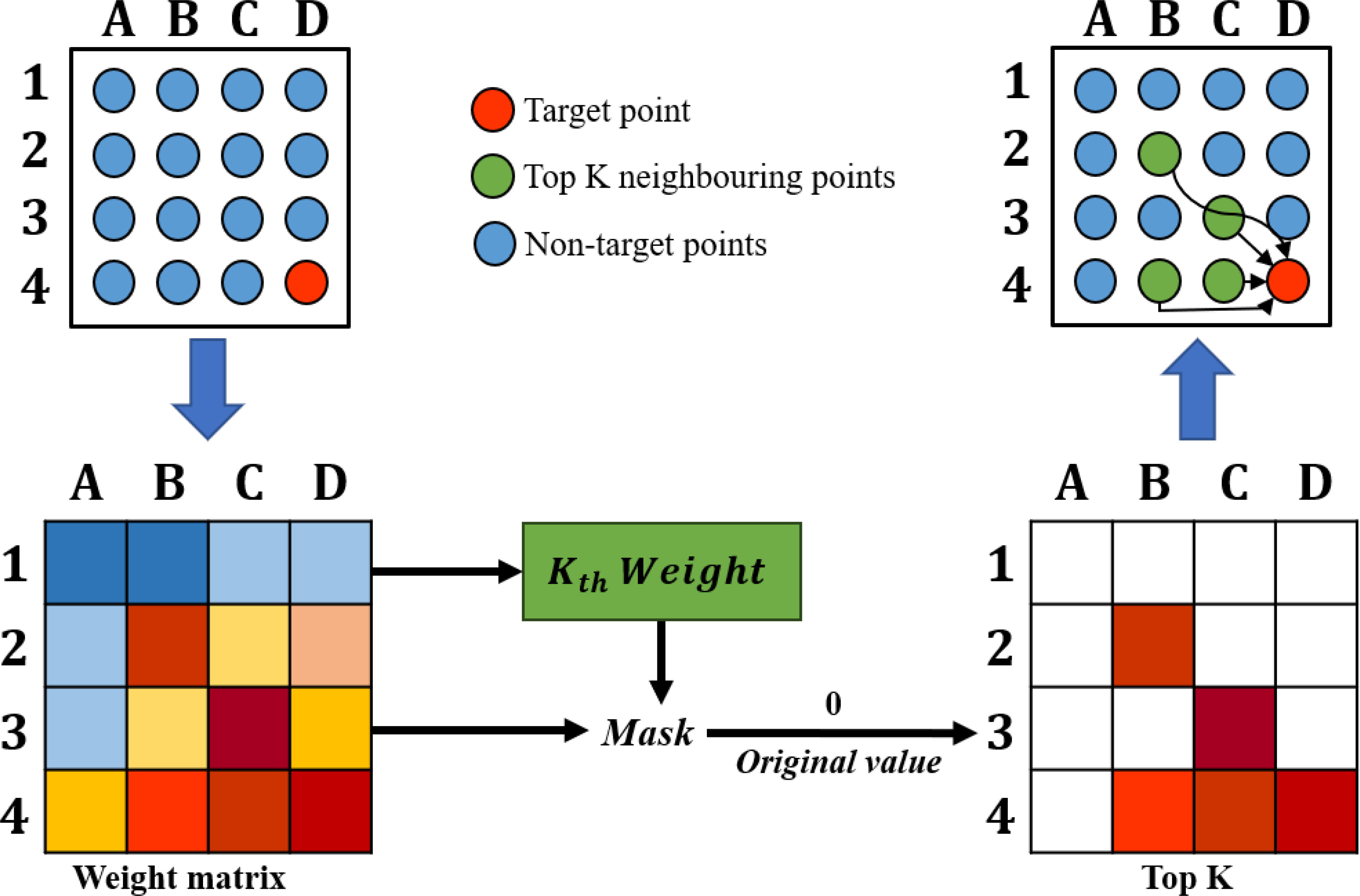
Figure 4 An illustration of the spatial information fusion in KSwin-T. The mask is obtained by calculating the kth weight value. The weak correlation weights are set to 0 and the high correlation weights are retained according to the mask.

4.2 Forecasting models based on KSwin-T and LSTM

Recurrent neural networks(RNN) modeling sequential data have proven successful in areas such as natural language processing and time series prediction. While the normal neural network only establishes weighted connections between layers, RNNs also establish weighted connections between neurons (Elman, 1990; Medsker and Jain, 2001). However, the issue of gradient vanishing or exploding frequently arises when computing connections between distant nodes (Pascanu et al., 2013). LSTM is a specialized variant of RNN whose hidden layer operates on matrices using a combination of several non-linear activation functions. The introduced memory cell in LSTM acts as an accumulator of state information which selectively passes time series information, input gate information, and forget gate information together, thus preventing gradient vanishing or exploding (Graves and Graves, 2012). Therefore, we use LSTM as the basic component of the ocean surface currents forecasting model.

In this study, an encoder-decoder model based on hybrid KSwin-T and LSTM is proposed for ocean surface currents forecasting, where neurons of the hybrid KSwin-T and LSTM are used as encoder while the decoder is constructed through LSTM only. Figure 5 illustrates the structure of the hybrid KSwin-T and LSTM neuron. Firstly, KSwin-T concatenates the input x_t at time t and the hidden state h_t−1 from the previous time step in the feature dimension using the f_concat function. Subsequently, KSwin-T utilizes the f_partition function to divide the data into multiple sub-regions of shape (S,S) in the spatial dimension, and modified self-attention computation is performed within each sub-region. The window partitioning is shifted across the multi-layer network, enabling the fusion of information between different sub-regions. Finally, multiple sub-regions are concatenated and restored through the f_reverse function. Mathematically, this process can be represented by Equations 1–4.

Figure 5

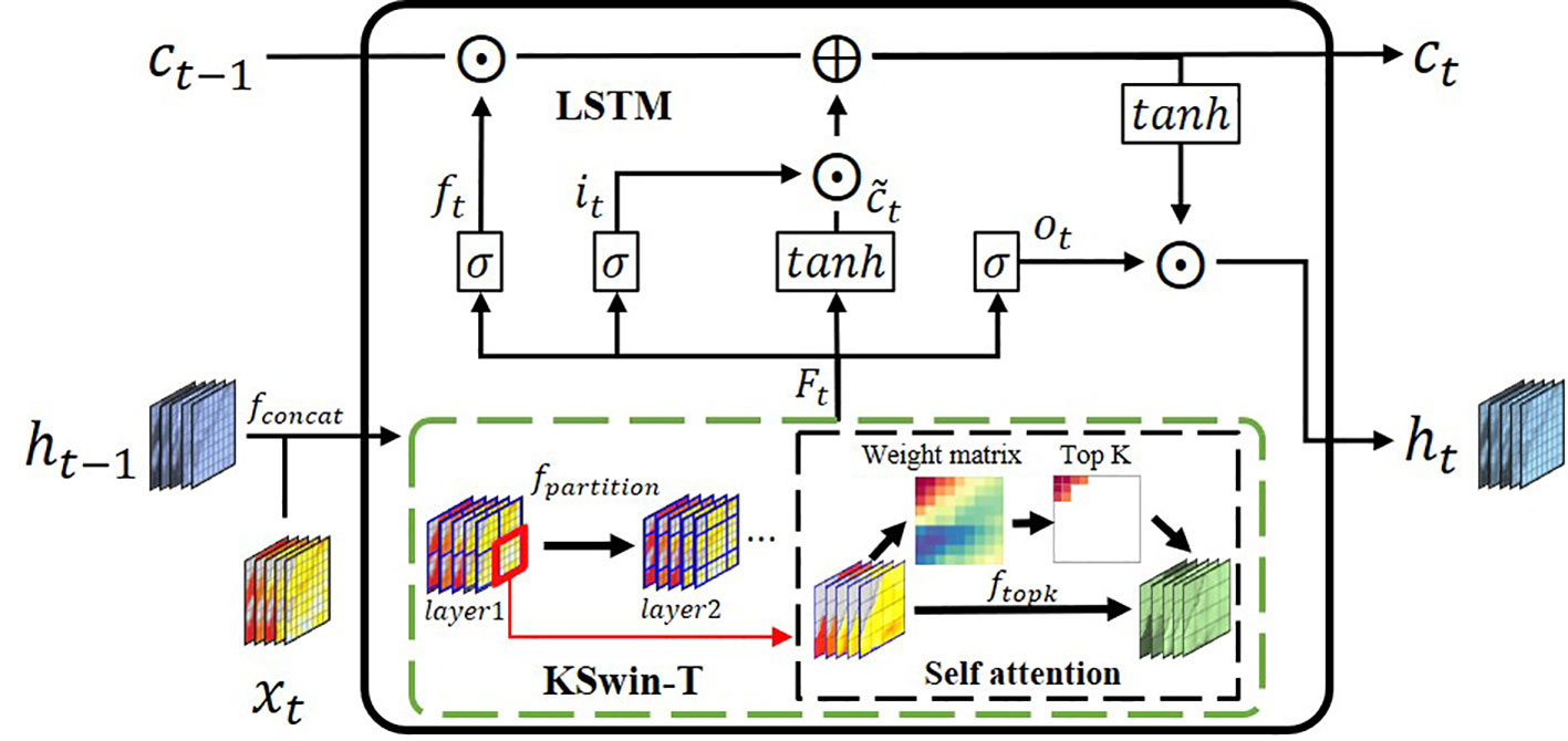
Figure 5 Schematic diagram of the hybrid KSwin-T and LSTM .

$\begin{array}{ll}{X}_t=f_{concat}(h_{t-1},x_t)& (1)\end{array}$

$\begin{array}{ll}{X}_t^r=f_{partition}(X_t,S)& (2)\end{array}$

$\begin{array}{ll}{F}_t^r=f_{topk}(X_t^r,K)& (3)\end{array}$

$\begin{array}{ll}{F}_t=f_{reverse}(F_t^r,S,H,W)& (4)\end{array}$

where f_concat denotes the feature concatenation function, f_partition represents the sub-region division function, r represents the r-th subregion, f_topk indicates a self-attention computation based on the KNN idea, and f_reverse represents the sub-region integration function. The above steps are all identified in Figure 5, and the subdivided sub-regions are shown by the red solid line boxes in it.

The data processed by the KSwin-T are fed into the LSTM to obtain the memory cell c_t and the hidden state h_t at the present moment. This process is repeated and eventually results in the hidden state h_T at the last time step T. The hidden state h_T serves as the initial input for the decoder LSTM, and the prediction results for the next T time steps are output during the iterative process. This process can be expressed by Equations 5–10.

$\begin{array}{ll}{i}_t=\sigma (F_t)& (5)\end{array}$

$\begin{array}{ll}{f}_t=\sigma (F_t)& (6)\end{array}$

$\begin{array}{ll}{o}_t=\sigma (F_t)& (7)\end{array}$

$\begin{array}{ll}{\tilde{c}}_t=\tanh (F_t)& (8)\end{array}$

$\begin{array}{ll}{c}_t=f_t☉c_{t-1}+i_t☉{\tilde{c}}_t& (9)\end{array}$

$\begin{array}{ll}{h}_t=o_t☉\tanh (c_t)& (10)\end{array}$

where σ represents the sigmoid function, tanh denotes the hyperbolic tangent function, and ⊙ signifies the operation of multiplying by elements, i.e. Hadamard product. The forget gate, input gate, and output gate are f_t, i_t, and o_t respectively. The memory cell at the previous and current moments are denoted as c_t−₁ and c_t, respectively.

In Figure 5, the feature dimension sizes of the previous time step’s hidden state h_t−1 and the current input x_t represent the number of ocean elements. After concatenation, they form X_t with a feature dimension size twice the number of ocean elements. In the process of self-attention computation, KSwin-T extracts features from X_t through multiple linear layers, thereby achieving the fusion of different ocean elements.

As shown in Figures 2 and 5, the fusion of ocean elements and spatial information occurs at each time step. During spatial information fusion, KSwin-T recalculates the weight matrix based on the current input X_t to capture the current spatial relationships of ocean currents. In this mechanism, the spatial self-attention weight matrix is different at different time steps and dynamically related to the current input X_t. Therefore, this is a dynamic spatiotemporal information fusion process.

Part (b) of Figure 2 depicts the spatiotemporal forecasting process, wherein the time series data x_t is sequentially fed into the encoder for encoding. The hidden state h_T at the final time step serves as the input to the decoder, which generates prediction results for the next T days.

During the model training, the mean absolute error (MAE) between the predictions and the labels is employed as the loss function, and the model parameters are updated through a backward process. When performing inference, this method applies denormalization to the model output to obtain accurate prediction results.

5 Experiments

This study employs three commonly used statistical and regression metrics to evaluate the performance of our proposed model: MAE, root mean square error (RMSE), mean normalized root mean square error (nRMSE), and correlation coefficient (r). The nRMSE captures the proportional relationship between the RMSE and the true values, thus evaluating the effectiveness of the predictions. The mathematical expressions for these evaluation indicators are shown in Equations 11–14.

$\begin{array}{ll}MAE=\frac{1}{H\times W}{\displaystyle \sum _{i=1}^H\sum _{j=1}^W\left|x_{ij}-y_{ij}\right|}& (11)\end{array}$

$\begin{array}{ll}RMSE=\sqrt{\frac{1}{H\times W}{\displaystyle \sum _{i=1}^H\sum _{j=1}^W{(x_{ij}-y_{ij})}^2}}& (12)\end{array}$

$\begin{array}{ll}nRMSE=\frac{RMSE}{\overline{x}}& (13)\end{array}$

$\begin{array}{ll}r=\frac{{\sum }_i^H{\sum }_j^W(x_{ij}-\overline{x})(y_{ij}-\overline{y})}{\sqrt{{\sum }_i^H{\sum }_j^W{(x_{ij}-\overline{x})}^2{\sum }_i^H{\sum }_j^W{(y_{ij}-\overline{y})}^2}}& (14)\end{array}$

where x_ij represents the true value, y_ij represents the predicted value, $\overline{x}$ denotes the mean of the true value, $\overline{y}$ denotes the mean of the predicted value, while H and W indicate the shape of the predicted region.

5.1 Hyper parameters

The encoder-decoder model based on hybrid KSwin-T and LSTM contains several crucial hyperparameters, namely the time window length T, the size of the self-attention window S, the number of layers in KSwin-T L, and the number of neighboring points chosen by KSwin-T K. In this study, we explored different values for these hyperparameters, including T ∈ {5,10,15}, S ∈ {5,10,20}, L ∈ {2,3,4}, and K ∈ {5,10,15}. It was observed that larger values of T improved long-term forecasting performance while sacrificing short-term forecasting accuracy. After experimenting, T = 15 was determined to strike a balance between short-term and long-term forecasting accuracy. Additionally, the combination of S = 20, L = 2, and K = 10 yielded the best performance.

The significance of S in ocean surface currents forecasting pertains to the size of the sub-region, while L represents the distance of information fusion between different sub-regions. In the spatial information fusion module, optimal direct fusion occurs for each sub-region when S closely matches the spatial scale of the currents. Meanwhile, L indirectly influences spatial information fusion by globally constraining the sliding range of the attention window. Considering the spatial accuracy of the data as 0.1°, setting S = 20 implies that the longitude and latitude span of the self-attention window is 2° × 2° in real geographic space. Furthermore, with L = 2, the indirect spatial information fusion is limited to neighboring sub-regions.

Figure 6 shows the spatial distribution of ocean surface currents speed in the study area. The blue area with the larger speed is the Kuroshio, which undergoes huge flow changes in eastern Taiwan and reveals a large difference in current speed from other areas (Chu, 1974; Hsin et al., 2008). In the figure, the sub-regions labeled as ①, ②, ③, and ④ represent the four adjacent regions divided by KSwin-T when S=20. These four regions exhibit different motion patterns at this specific time. The first layer of KSwin-T effectively divides them to mitigate mutual interference during direct spatial information fusion. In addition, the second layer of KSwin-T further divided the region into a new sub-region labeled as ④, which is positioned at the junction of the four regions. This enables the fusion of spatial information about the eddy current present at this particular junction.

Figure 6

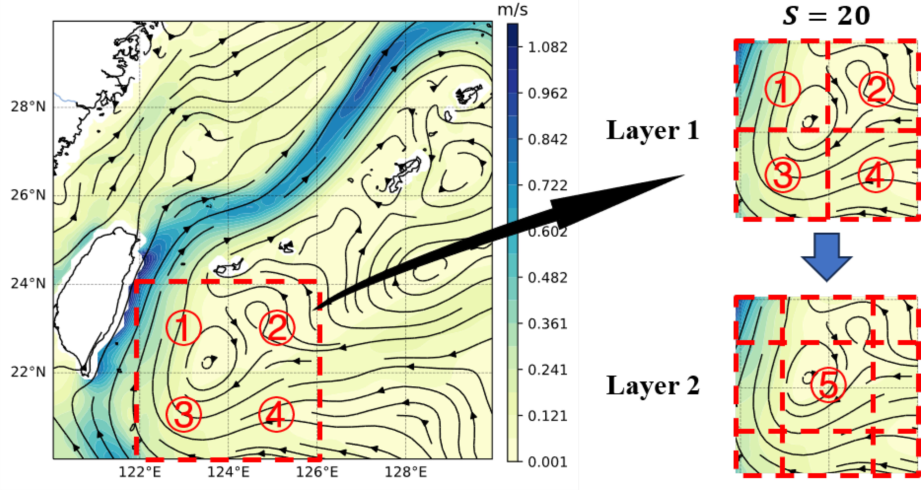
Figure 6 Self-attention window partitioning of the study area by KSwin-T at S=20.

In addition to the aforementioned key hyperparameters, there are several other essential hyperparameters that must be configured for our model. To balance the generalization performance and the prediction performance of the model, the dropout layer’s rate in the network is set to 0.2. The learning rate during model training is set to 0.001, and the batch size is set to 8.

5.2 Ablation study

5.2.1 The effectiveness of the KSwin-T

To verify the effectiveness of KSwin-T, we conducted a comparison experiment with the normal Swin-T. Specifically, we compared the differences between the two during training and testing, respectively. Except for this part, the parameter settings of the model were kept consistent.

The loss curves during the training process for KSwin-T and Swin-T, as depicted in Figure 7A, indicate that Swin-T exhibits a faster decrease in loss during training, and the final converged loss is significantly smaller than that of KSwin-T. This strongly suggests the superior fitting ability of Swin-T to the input ocean flow data. However, examining the Mean Absolute Error (MAE) curves for the U and V directions in the test set, as shown in Figures 7B, C, reveals that despite Swin-T’s better fitting performance during training, it experiences larger errors. This implies that, in comparison to Swin-T, KSwin-T demonstrates better generalization ability, while Swin-T exhibits signs of overfitting.

Figure 7

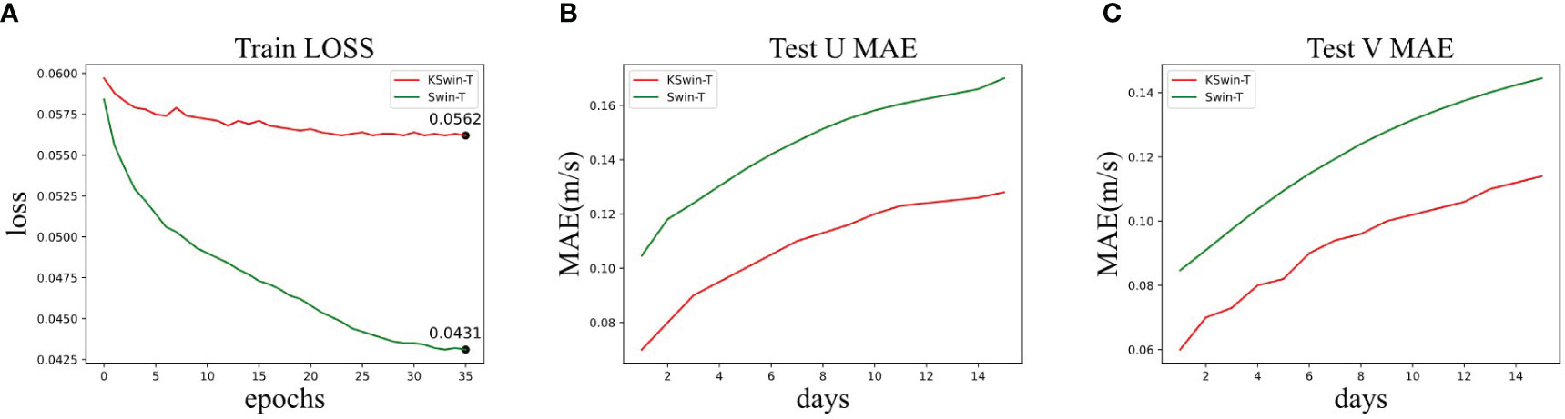
Figure 7 (A) Loss variation curves of the spatiotemporal forecasting model using KSwin-T with Swin-T during the training process. (B) U-component velocity MAE for lead times of 1 to 15 days during the test. (C) V-component velocity MAE for lead times of 1 to 15 days during the test.

In order to observe the spatial information fusion effect of KSwin-T, we visualized the self-attention weights of sub-region ① in Figure 6 while performing spatiotemporal forecasts. Figure 8A shows the enlarged display of sub-region ①, where the target point (22°N,122.4°E) is at the junction of the left northward Kuroshio and the right eddy, which is jointly influenced by both sides. Figure 8B shows the weight matrix corresponding to the five self-attention heads of the sub-region in the multi-head self-attention process. Since the shape of sub-regions is (20, 20), the corresponding weight matrix is shaped as (400,400), where the i-th row indicates the weight of the i-th point with the 400 points of the whole region.

Figure 8

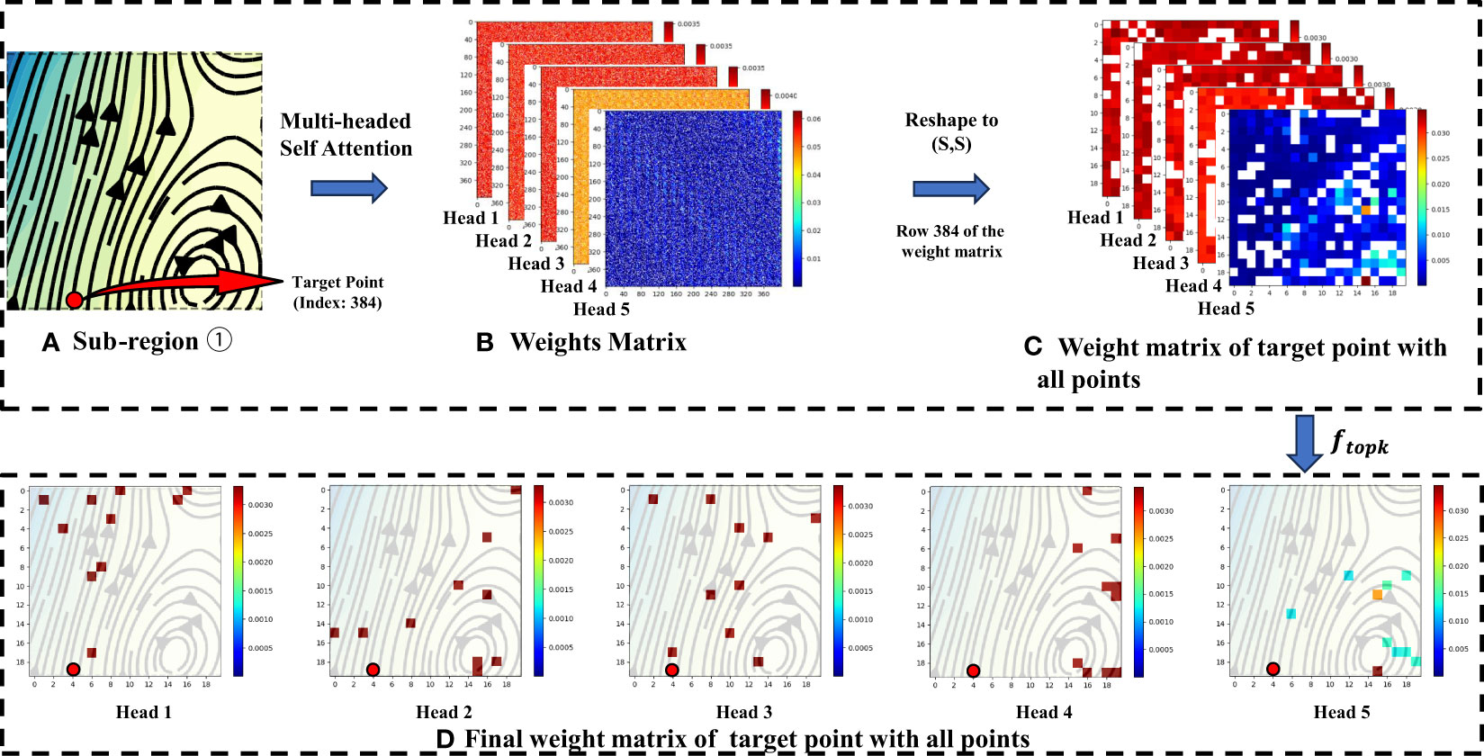
Figure 8 (A) The enlarged display of sub-region ① in Figure 6. (B) Weight matrix for sub-region ① obtained by multi-headed self-attention. (C) Weight matrix of target point in Figure 8A with all points in the sub-region ①. (D) The matrix of weights retained after the Top K selection operation.

The weights corresponding to the target point in Figure 8A, i.e., the 384-th row of the weight matrix, are reshaped to the weight matrix in Figure 8C. It can be found that the number of highly correlated points in the weight matrix is small, and most of the points are weakly correlated points, and these weakly correlated points will introduce interference information in the process of spatial information fusion.

Therefore, we only take the top K points with high correlation for spatial information fusion, and the retained points are shown in Figure 8D. It can be observed that the K fusion points retained by Head1 are mainly concentrated in the far end of the Kuroshio Current, indicating that Head1 pays more attention to the impact of the Kuroshio on the target points during self-attention computation. Similarly, we can see that Head2 and Head3 focus more on the impact of the convergence area between the Kuroshio and eddies on the target points, while Head4 and Head5 are more concerned with the influence of the eddy region on the right side on the target points. The different attention heads, along with the retained K points, effectively cover the spatial patterns of ocean currents in this scenario.

Furthermore, KSwin-T serves as a spatial information fusion technique for the input currents field at any given time. As the input currents field changes, the self-attention weights adjust accordingly. Consequently, KSwin-T emerges as an adaptive spatial information fusion method, showcasing exceptional performance in capturing the dynamic spatial relationships within ocean currents.

5.2.2 Analysis of multi-element feature fusion

As shown in Table 1, experiments were set up based on five elements, including U and V components of ocean surface currents, SST, SSS, and SSH. The best forecasting results were achieved when all five elements were input into the model simultaneously for multi-element fusion. Surface currents are influenced by many factors, of which temperature and salinity influence the three-dimensional ocean circulation by changing the density of seawater (Willmott, 2016). Due to the large amount of heat transported from the tropics to the mid-latitudes by the Kuroshio (Qiu and Chen, 2010), temperature plays a dominant role in affecting the ocean currents while salinity seems to be non-negative (Qu and Lukas, 2003; Chen et al., 2022). The experimental results show that the combination of SST or SSS has a lower forecast error, which is consistent with the above conclusions. In addition, SSH is also one of the relevant elements of ocean surface currents which can reflect the movement of surface currents. The altimeters are also commonly used to estimate surface currents (Lagerloef et al., 1999; Bonjean and Lagerloef, 2002; Johnson et al., 2002; Cao et al., 2023b), so the forecasting effect is significantly enhanced by adding SSH.

Table 1

Table 1 MAE results for different combinations of ocean elements as inputs to ASTMEN for the U- and V-component of ocean current velocity.

Figure 9 shows the analysis of variance for each point in the time dimension. It can be seen that U’s variance is larger than V’s variance in the time dimension, indicating that U varies more dramatically overtime at T = 15 days. This finding is consistent with the experimental results in Table 1 where the forecast error for U is always higher. Even so, ASTMEN achieves excellent forecasting performance through the fusion of multi-element information. The ablation study of multi-element fusion demonstrates that SST, SSS, and SSH have a synergistic changes with ocean currents, which is consistent with previous oceanographic studies. Therefore it is necessary to fuse other relevant ocean elements in the process of forecasting ocean surface currents.

Figure 9

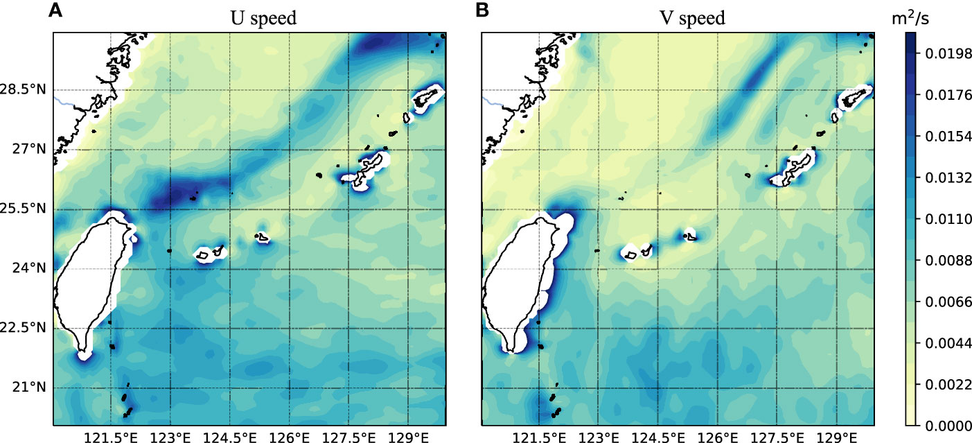
Figure 9 The time-dimensional variance of the ocean surface current velocity at each point in space over T days, where T is the length of the time window for the inputs and outputs of the model, i.e. T = 15.

5.3 Baseline algorithm

In order to evaluate the performance of ASTMEN in forecasting ocean surface currents, five algorithms are compared, of which LSTM, CNN-GRU and ConvLSTM have been shown to be effective for spatial and temporal forecasting of ocean surface currents (Thongniran et al., 2019; Immas et al., 2021; Liu et al., 2022). This study also adds the climate state calculated from the CORA 2.0 reanalysis dataset during 2015-2018 as a comparison, to verify the effectiveness of ASTMEN. All models in this study are implemented using python 3.8 and PyTorch (Paszke et al., 2019), and our experimental and validation environment is built as follows: Intel(R) Xeon(R) Silver 4210 CPU @ 2.20GHz with GeForce RTX 2080 Ti GPU, 64G RAM, and Ubuntu 18.04.

6 Results and analysis

6.1 Performance study

Table 2 presents the performance of ASTMEN compared with the baseline model based on four key statistical indicators at days 1-15, respectively, and the best model is marked in bold. The results show that ASTMEN has a lower MAE, RMSE, and nRMSE, as well as a higher correlation coefficient over the 15 days of continuous forecasting. It can also be observed that the advantage of ASTMEN is not obvious on the first day, but the rate of error accumulation of ASTMEN is much smaller than that of other methods so the advantage becomes obvious after three days. This is because the changes of ocean currents in the short term are simpler and can be well captured by methods with weak spatial information fusion or methods without spatial information fusion such as LSTM. In short-term currents forecasting, spatial information can become a noise that leads to sub-optimal predictions, and as the duration of the forecast increases, current changes become more complex. Therefore, ASTMEN which has excellent spatial information fusion capability shows better forecast performance in continuous forecasting and still achieves a correlation coefficient of 80% on the 12-th day of the forecast.

Table 2

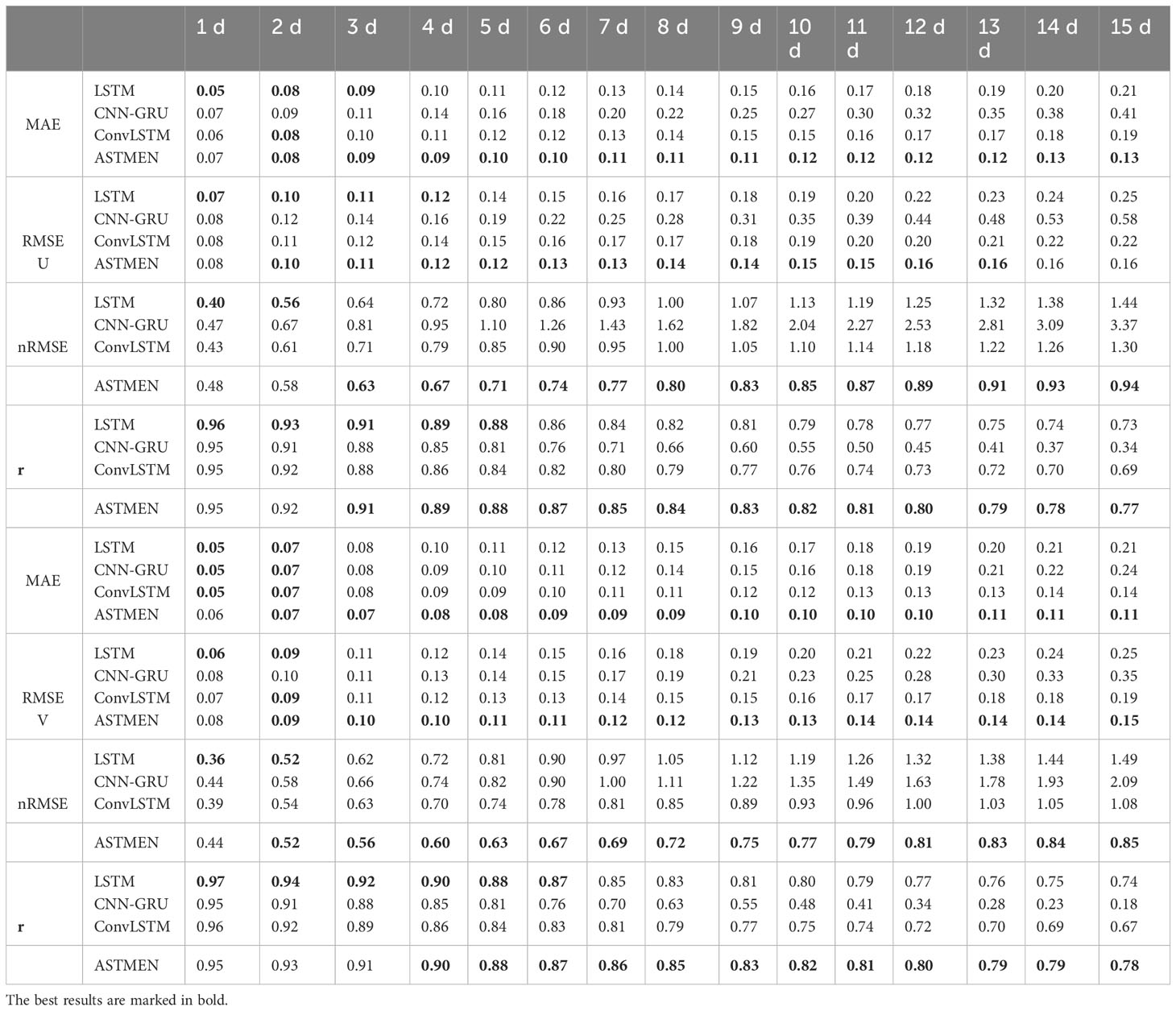
Table 2 Performance results of ASTMEN and baseline models on the U- and V-components of the ocean current velocity, with different lead times.

The variations of nRMSE for different prediction models over a forecast lead time of 1-15 days are detailed in Figure 10. From the graphs, it can be observed that ASTMEN exhibits a significantly lower rate of error accumulation over the entire 15-day forecasting process compared to the baseline model. This provides strong evidence for the outstanding effectiveness of adaptive spatiotemporal information fusion in ocean surface currents forecasting. Additionally, it can be noted that for the fifteenth day, ASTMEN is the only model with an nRMSE value less than 1, indicating that the RMSE at this point is lower than the mean speed of the ocean currents. The effectiveness of the proposed method is also further confirmed by comparison with climate state predictions.

Figure 10

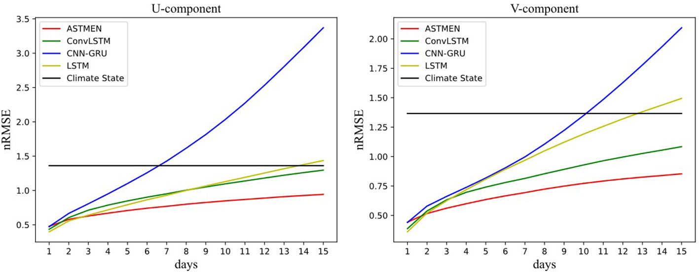
Figure 10 The nRMSE curves for ASTMEN and baseline models over a 15-day continuous prediction period.

Figure 11 depicts the distribution relationship between the predicted values and the true values in the test set. Specifically, the scatter plots show the predicted and the true current velocities of ASTMEN and ConvLSTM for days 1, 3, 5, 7, 10 and 15 of the continuous prediction process. The horizontal axis of the scatter plot represents the true flow velocity of the samples in the test set, while the vertical axis represents the predicted flow velocity of the samples in the test set. As shown in the graph, the closer the points are to the diagonal line, the better the prediction, indicating a closer alignment between the predicted values and the actual values. The distribution of points for ASTMEN is more concentrated around the diagonal line, whereas ConvLSTM exhibits a large number of scattered points deviating from the diagonal line after the first day. The horizontal coordinates of most of these scattered points are close to 0, indicating that forecast errors are instead higher at points with lower actual current velocities. Based on previous oceanographic studies and the distribution of the current field in Figure 6, the currents in the regions with higher velocities tend to be more stable and have a single pattern, while the currents in the regions with lower velocities show more complex patterns and more turbulent current directions. The conclusions indicate that ConvLSTM is less effective in these regions with unstable currents. In contrast, ASTMEN shows superior performance in areas with complex and variable ocean currents.

Figure 11

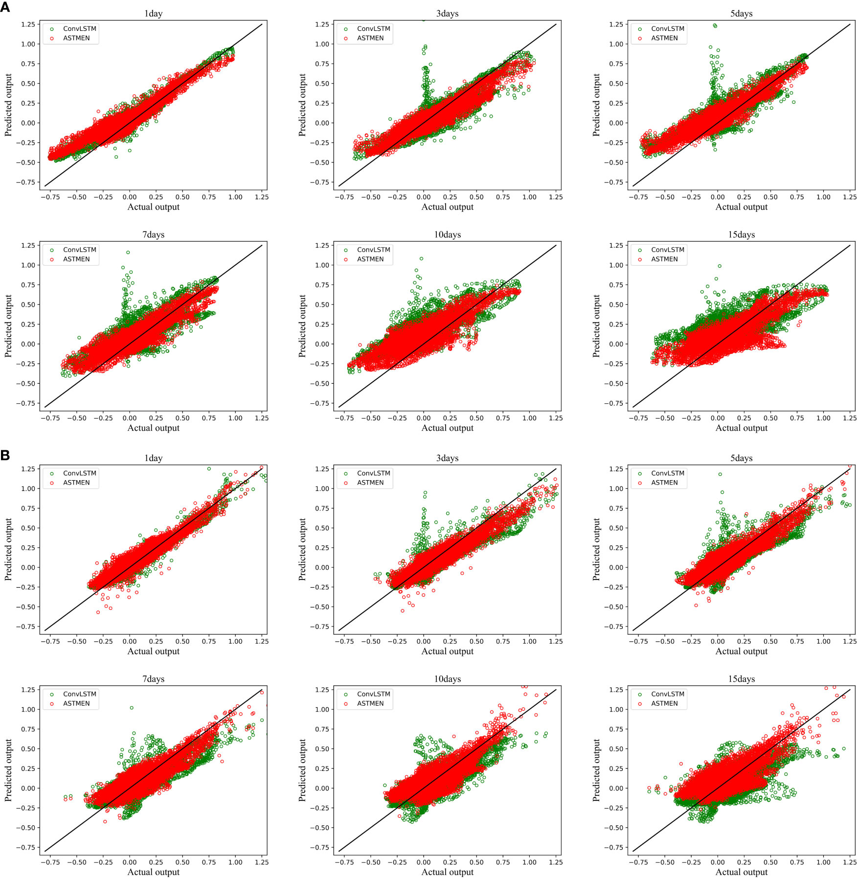
Figure 11 Scatter plot of predicted current velocities and true current velocities. The predicted Ucomponent and V-component results of ASTMEN and ConvLSTM at 1, 3, 5, 7, 10, and 15 days ahead are shown, respectively. (A) The U-component scatter plot. (B) The V-component scatter plot.

6.2 Case study

Figure 12 shows the daily spatial dimensional variance for the different seasons, obtained by calculating the average of the daily variance over the period 2015-2018. It can be observed that the spatial dimensional variance is much higher in summer than in other seasons, implying that the spatial patterns of ocean currents are more complex and more difficult to be forecasted in summer. To evaluate the performance of the model under the complex variability of ocean currents, we conducted experiments specifically for the summer currents. We used the ocean currents data from June 1, 2019, to June 15, 2019, as input and performed continuous forecasting of the ocean currents from June 16, 2019, to June 30, 2019. The experimental setup remained unchanged to ensure consistency.

Figure 12

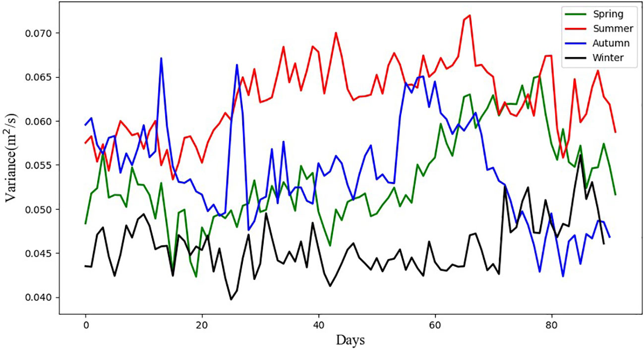
Figure 12 Daily spatial dimensional variance curves for the study area in different seasons. Variance values are averaged over the period 2015-2018.

Based on the experimental results, the study area can be divided into the four sub-regions presented in Figure 1 for discussion, which are the East China Sea, the Kuroshio, the Ryukyu Islands and the Philippine Sea. Figure 13 presents the residual maps of ASTMEN and the baseline model for the dates June 16, June 18, June 20, June 22, June 25, and June 30. The results of the climate state forecasts have low errors in the East China Sea and high errors in the other three sub-regions, which implies that the inter-annual changes of the surface currents in the East China Sea are small, while the surface currents in the other three regions are more variable.

Figure 13

Figure 13 Residual heat map of the predicted and real ocean currents. The U-component and V-component residual results for ASTMEN and baseline models at 2019.06.16, 2019.06.18, 2019.06.20, 2019.06.22, 2019.06.25 and 2019.06.30 are shown, respectively. (A) The U-component residual results. (B) The V-component residual results.

In addition, several methods exhibit high forecast errors, especially CNN-GRU, in the eddy region of the Philippine Sea and along the coasts of the Ryukyu Islands and Taiwan Islands. This is because CNN-GRU uses a two-stage structure with separate spatial information fusion and temporal feature extraction, which cannot dynamically fuse spatial information according to temporal changes during the continuous prediction, resulting in high forecast errors for complex ocean currents. It can also be found that ConvLSTM shows high anomalies at the junction of land and sea, such as the east coast of Taiwan, where the Kuroshio is blocked by land and turns, resulting in large changes in both the velocity and direction of the currents. However, the fixed size and parameters of the convolution kernel of the ConvLSTM are unable to make adaptive changes for a particular current pattern, which leads to worse prediction results. On the contrary, due to the high stability of the inter-annual variability of the Kuroshio, the LSTM achieves better forecasting results here.

Meanwhile, according to Figure 9, it can also be found that the time dimension variance tends to be large in the regions with larger errors. However, ASTMEN achieves lower forecast errors than other methods, in the East China Sea and in the Kuroshio, where currents are stable, and in the eddy and land-sea interface regions, where changes are intense. In some special current conditions, such as the Kuroshio turning under the influence of land, ASTMEN is still able to capture this change adaptively and achieve a more accurate and continuous forecast.

7 Conclusions

In this paper, we propose a surface currents forecasting model based on the adaptive spatiotemporal information fusion and multi-element fusion neural network, and this model effectively solves the problems of the complex and variable spatial structure of ocean currents, which are affected by various oceanographic factors and make it difficult to improve forecast accuracy. And the sea area of eastern China with complex spatial structure was selected as the study area, while experiments and analyses were conducted on the CORA2.0 reanalysis dataset. Benefiting from the adaptive spatial information fusion and multi-element feature fusion of KSwin-T, ASTMEN has a clear advantage in error reduction during the continuous forecasting process over the baseline model, as well as in the forecasting of the ocean-land interface and regional edges. For forecasts 15 days ahead, the average nRMSE of ASTMEN is still less than 1.0, which has high validity and provides a better prediction method for offshore activities. By visualizing the forecast results of the ocean surface currents in the study area for the period 2019.06.16-2019.06.30, it is visually noticed that ASTMEN is more effective at the interface between ocean and land and in the eddy region where the currents pattern is more complex. In addition, the comparison with climate state prediction also demonstrates the effectiveness of ASTMEN for ocean surface currents prediction. The limitations of ASTMEN are the complexity of the model and multiple hyperparameters that need to be determined by experiment. Moreover, ASTMEN has less advantage in the short term, which we believe is due to the small variability of ocean currents over short periods of time, which is overestimated by ASTMEN, thus reducing forecast performance. Therefore, future work will address the complexity of the model. Furthermore, we did not explore the specific interaction principles between different ocean elements in detail, which may overlook some physical relationships that have been quantified, and the effectiveness of multi-element fusion can be improved in future studies by introducing these specific physical parameters. Notably, this study is based on a single area and uses a reanalysis dataset with a more complete initial field, which is slightly different from the ocean data observed in real-time, but ASTMEN can extract sufficient potential information from the data so that it is theoretically applicable to real-time observations as well as to other areas, which we will verify in future work.

Data availability statement

The original contributions presented in the study are included in the article/supplementary materials, further inquiries can be directed to the corresponding author/s.

Author contributions

XL: Conceptualization, Formal analysis, Methodology, Writing – original draft, Writing – review & editing. FW: Data curation, Software, Validation, Writing – original draft. TS: Formal analysis, Supervision, Writing – original draft, Writing – review & editing. FM: Formal analysis, Investigation, Supervision, Writing – review & editing. XZ: Validation, Writing – original draft.

Funding

The author(s) declare financial support was received for the research, authorship, and/or publication of this article. This work was supported by grants of the Natural Science Foundation of Shandong Province of China (Project No. ZR2020MF140) and the Key Laboratory of Marine Hazard Forecasting, Ministry of Natural Resources (Project No. LOMF2202).

Conflict of interest

The authors declare that the research was conducted in the absence of any commercial or financial relationships that could be construed as a potential conflict of interest.

Publisher’s note

All claims expressed in this article are solely those of the authors and do not necessarily represent those of their affiliated organizations, or those of the publisher, the editors and the reviewers. Any product that may be evaluated in this article, or claim that may be made by its manufacturer, is not guaranteed or endorsed by the publisher.

References

Bethel B. J., Sun W., Dong C., Wang D. (2022). Forecasting hurricane-forced significant wave heights using a long short-term memory network in the caribbean sea. Ocean Sci. 18, 419–436. doi: 10.5194/os-18-419-2022

CrossRef Full Text | Google Scholar

Bleck R. (2002). An oceanic general circulation model framed in hybrid isopycnic-cartesian coordinates. Ocean Model. 4, 55–88. doi: 10.1016/S1463-5003(01)00012-9

CrossRef Full Text | Google Scholar

Blumberg A. F., Mellor G. L. (1987). A description of a three-dimensional coastal ocean circulation model. Three-dimensional Coast. ocean Models 4, 1–16. doi: 10.1029/CO004p0001

CrossRef Full Text | Google Scholar

Bolton T., Zanna L. (2019). Applications of deep learning to ocean data inference and subgrid parameterization. J. Adv. Modeling Earth Syst. 11, 376–399. doi: 10.1029/2018MS001472

CrossRef Full Text | Google Scholar

Bonjean F., Lagerloef G. S. (2002). Diagnostic model and analysis of the surface currents in the tropical pacific ocean. J. Phys. Oceanography 32, 2938–2954. doi: 10.1175/1520-0485(2002)032<2938:DMAAOT>2.0.CO;2

CrossRef Full Text | Google Scholar

Cao Y., Dong C., Stegner A., Bethel B. J., Li C., Dong J., et al. (2023b). Global sea surface cyclogeostrophic currents derived from satellite altimetry data. J. Geophysical Research: Oceans 128, e2022JC019357. doi: 10.1029/2022JC019357

CrossRef Full Text | Google Scholar

Cao H., Liu G., Huo J., Gong X., Wang Y., Zhao Z., et al. (2023a). Multi factors-predrnn based significant wave height prediction in the bohai, yellow, and east China seas. Front. Mar. Sci. 10. doi: 10.3389/fmars.2023.1197145

CrossRef Full Text | Google Scholar

Chelton D. B., Schlax M. G., Samelson R. M. (2011). Global observations of nonlinear mesoscale eddies. Prog. Oceanography 91, 167–216. doi: 10.1016/j.pocean.2011.01.002

CrossRef Full Text | Google Scholar

Chen C., Beardsley R. C., Cowles G. (2006). An unstructured grid, finite-volume coastal ocean model (fvcom) system. Oceanography 19, 78–89. doi: 10.5670/oceanog.2006.92

CrossRef Full Text | Google Scholar

Chen C., Shiotani S., Sasa K. (2015). Effect of ocean currents on ship navigation in the east China sea. Ocean Eng. 104, 283–293. doi: 10.1016/j.oceaneng.2015.04.062

CrossRef Full Text | Google Scholar

Chen L., Zhang R.-H., Gao C. (2022). Effects of temperature and salinity on surface currents in the equatorial pacific. J. Geophysical Research: Oceans 127, e2021JC018175. doi: 10.1029/2021JC018175

CrossRef Full Text | Google Scholar

Choi J. M., Kim W., Hong T. T. M., Park Y.-G. (2021). Derivation and evaluation of satellite-based surface current. Front. Mar. Sci. 8, 695780. doi: 10.3389/fmars.2021.695780

CrossRef Full Text | Google Scholar

Chu T. (1974). The fluctuations of the kuroshio current in the eastern sea area of Taiwan. Acta Oceanogr Taiwanica 4, 1–12.

Google Scholar

Cover T., Hart P. (1967). Nearest neighbor pattern classification. IEEE Trans. Inf. Theory 13, 21–27. doi: 10.1109/TIT.1967.1053964

CrossRef Full Text | Google Scholar

Dosovitskiy A., Beyer L., Kolesnikov A., Weissenborn D., Zhai X., Unterthiner T., et al. (2020). An image is worth 16x16 words: transformers for image recognition at scale. in International Conference on Learning Representations.

Google Scholar

Elman J. L. (1990). Finding structure in time. Cogn. Sci. 14, 179–211. doi: 10.1207/s15516709cog1402_1

CrossRef Full Text | Google Scholar

Graves A., Graves A. (2012). Long short-term memory. Supervised sequence labelling recurrent Neural Networks 385, 37–45. doi: 10.1007/978-3-642-24797-2_4

CrossRef Full Text | Google Scholar

Griffies S. M., Gnanadesikan A. W. D. K., Dixon K. W., Dunne J. P., Zhang R. (2005). Formulation of an ocean model for global climate simulations. Ocean Sci. 1, 45–79. doi: 10.5194/os-1-45-2005

CrossRef Full Text | Google Scholar

Gu Z., Chai X., Yang T. (2023). Deep-learning-based low-frequency reconstruction in full-waveform inversion. Remote Sens. 15, 1387. doi: 10.3390/rs15051387

CrossRef Full Text | Google Scholar

Halpern B. S., Frazier M., Afflerbach J., Lowndes J. S., Selkoe K. A. (2019). Recent pace of change in human impact on the world’s ocean. Sci. Rep. 9, 11609. doi: 10.1038/s41598-019-47201-9

PubMed Abstract | CrossRef Full Text | Google Scholar

Hsin Y.-C., Wu C.-R., Shaw P.-T. (2008). Spatial and temporal variations of the kuroshio east of Taiwan 1982–2005: A numerical study. J. Geophysical Research: Oceans 113.

Google Scholar

Immas A., Do N., Alam M. R. (2021). Real-time in situ prediction of ocean currents. Ocean Eng. 228, 108922. doi: 10.1016/j.oceaneng.2021.108922

CrossRef Full Text | Google Scholar

Jin B., Wang G., Liu Y., Zhang R. (2010). Interaction between the east China sea kuroshio and the ryukyu current as revealed by the self-organizing map. J. Geophysical Res. Oceans 115, C12047:1-C12047:7. doi: 10.1029/2010JC006437

CrossRef Full Text | Google Scholar

Johnson G. C., Sloyan B. M., Kessler W. S., McTaggart K. E. (2002). Direct measurements of upper ocean currents and water properties across the tropical pacific during the 1990s. Prog. Oceanography 52, 31–61. doi: 10.1016/S0079-6611(02)00021-6

CrossRef Full Text | Google Scholar

Jrges C., Berkenbrink C., Stumpe B. (2021). Prediction and reconstruction of ocean wave heights based on bathymetric data using lstm neural networks. Ocean Eng. 232. doi: 10.1016/j.oceaneng.2021.109046

CrossRef Full Text | Google Scholar

Khosravi A., Koury R. N. N., MaChado L., Pabon J. J. G. (2018). Prediction of wind speed and wind direction using artificial neural network, support vector regression and adaptive neuro-fuzzy inference system. Sustain. Energy Technol. Assessments 25, 146–160. doi: 10.1016/j.seta.2018.01.001

CrossRef Full Text | Google Scholar

Lagerloef G. S., Mitchum G. T., Lukas R. B., Niiler P. P. (1999). Tropical pacific near-surface currents estimated from altimeter, wind, and drifter data. J. Geophysical Research: Oceans 104, 23313–23326. doi: 10.1029/1999JC900197

CrossRef Full Text | Google Scholar

Lermusiaux P. F. J. (2006). Uncertainty estimation and prediction for interdisciplinary ocean dynamics. J. Comput. Phys. 217, 176–199. doi: 10.1016/j.jcp.2006.02.010

CrossRef Full Text | Google Scholar

Li Z.-L., Yu J., Zhang X.-L., Xu L.-Y., Jin B.-G. (2022). A multi-hierarchical attention-based prediction method on time series with spatio-temporal context among variables. Physica A: Stat. Mechanics its Appl. 602, 127664. doi: 10.1016/j.physa.2022.127664

CrossRef Full Text | Google Scholar

Liu M., Chen R., Guan W., Zhang H., Jing T. (2023). Nonlocality of scale-dependent eddy mixing at the kuroshio extension. Front. Mar. Sci. 10, 1137216. doi: 10.3389/fmars.2023.1137216

CrossRef Full Text | Google Scholar

Liu Z., Lin Y., Cao Y., Hu H., Wei Y., Zhang Z., et al. (2021). “Swin transformer: Hierarchical vision transformer using shifted windows,” in Proceedings of the IEEE/CVF international conference on computer vision. 10012–10022.

Google Scholar

Liu J., Yang J., Liu K., Xu L. (2022). Ocean current prediction using the weighted pure attention mechanism. J. Mar. Sci. Eng. 10. doi: 10.3390/jmse10050592

CrossRef Full Text | Google Scholar

Medsker L. R., Jain L. (2001). Recurrent neural networks. Design Appl. 5, 64–67.

Google Scholar

Meng F., Song T., Xu D., Xie P., Li Y. (2021). Forecasting tropical cyclones wave height using bidirectional gated recurrent unit. Ocean Eng. 234, 108795. doi: 10.1016/j.oceaneng.2021.108795

CrossRef Full Text | Google Scholar

Meng F., Xu D., Song T. (2022). Atdnns: An adaptive time–frequency decomposition neural networkbased system for tropical cyclone wave height real-time forecasting. Future Generation Comput. Syst. 133, 297–306. doi: 10.1016/j.future.2022.03.029

CrossRef Full Text | Google Scholar

Moore A. M., Arango H. G., Broquet G., Powell B. S., Weaver A. T., Zavala-Garay J. (2011). The regional ocean modeling system (roms) 4-dimensional variational data assimilation systems: Part i–system overview and formulation. Prog. Oceanography 91, 34–49. doi: 10.1016/j.pocean.2011.05.004

CrossRef Full Text | Google Scholar

Noori R., Abbasi M. R., Adamowski J. F., Dehghani M. (2017). A simple mathematical model to predict sea surface temperature over the northwest Indian ocean. Estuar. Coast. Shelf Sci. 197, 236–243. doi: 10.1016/j.ecss.2017.08.022

CrossRef Full Text | Google Scholar

Özturk Ş., Özkaya U., Akdemir B., Seyfi L. (2018). “Convolution kernel size effect on convolutional neural network in histopathological image processing applications,” in 2018 International Symposium on Fundamentals of Electrical Engineering (ISFEE) (IEEE). 1–5.

Google Scholar

Pascanu R., Mikolov T., Bengio Y. (2013). “On the difficulty of training recurrent neural networks,” in International conference on machine learning (Pmlr).

Google Scholar

Paszke A., Gross S., Massa F., Lerer A., Bradbury J., Chanan G., et al. (2019). Pytorch: An imperative style, high-performance deep learning library. Adv. Neural Inf. Process. Syst. 32, 8026–8037.

Google Scholar

Peng Q., Xie S.-P., Wang D., Huang R. X., Chen G., Shu Y., et al. (2022). Surface warming–induced global acceleration of upper ocean currents. Sci. Adv. 8, eabj8394. doi: 10.1126/sciadv.abj8394

PubMed Abstract | CrossRef Full Text | Google Scholar

Portillo Juan N., Negro Valdecantos V. (2022). Review of the application of artificial neural networks in ocean engineering. Ocean Eng. 259, 111947. doi: 10.1016/j.oceaneng.2022.111947

CrossRef Full Text | Google Scholar

Qiu B., Chen S. (2010). Interannual-to-decadal variability in the bifurcation of the north equatorial current off the Philippines. J. Phys. Oceanography 40, 2525–2538. doi: 10.1175/2010JPO4462.1

CrossRef Full Text | Google Scholar

Qu T., Lukas R. (2003). The bifurcation of the north equatorial current in the pacific. J. Phys. Oceanography 33, 5–18. doi: 10.1175/1520-0485(2003)033<0005:TBOTNE>2.0.CO;2

CrossRef Full Text | Google Scholar

Remya P. G., Kumar R., Basu S. (2012). Forecasting tidal currents from tidal levels using genetic algorithm. Ocean Eng. 40, 62–68. doi: 10.1016/j.oceaneng.2011.12.002

CrossRef Full Text | Google Scholar

Roemmich D., Gilson J. (2009). The 2004–2008 mean and annual cycle of temperature, salinity, and steric height in the global ocean from the argo program. Prog. Oceanography 82, 81–100. doi: 10.1016/j.pocean.2009.03.004

CrossRef Full Text | Google Scholar

Rozier D., Birol F., Cosme E., Brasseur P., Verron J. M. B. (2007). A reduced-order kalman filter for data assimilation in physical oceanography. SIAM Rev. 449–465. doi: 10.1137/050635717

CrossRef Full Text | Google Scholar

Shchepetkin A. F., McWilliams J. C. (2005). The regional oceanic modeling system (roms): a splitexplicit, free-surface, topography-following-coordinate oceanic model. Ocean Model. 9, 347–404. doi: 10.1016/j.ocemod.2004.08.002

CrossRef Full Text | Google Scholar

Sinha A., Abernathey R. (2021). Estimating ocean surface currents from satellite observable quantities with machine learning. Front. Mar. Sci. 8. doi: 10.31223/X5PK74

CrossRef Full Text | Google Scholar

Song T., Wang Z., Xie P., Han N., Jiang J., Xu D. (2020). A novel dual path gated recurrent unit model for sea surface salinity prediction. J. Atmospheric Oceanic Technol. 37, 317–325. doi: 10.1175/JTECH-D-19-0168.1

CrossRef Full Text | Google Scholar

Sun W., Zhou S., Yang J., Gao X., Ji J., Dong C. (2023). Artificial intelligence forecasting of marine heatwaves in the south China sea using a combined u-net and convlstm system. Remote Sens. 15, 4068. doi: 10.3390/rs15164068

CrossRef Full Text | Google Scholar

Thongniran N., Vateekul P., Jitkajornwanich K., Lawawirojwong S., Srestasathiern P. (2019). “Spatiotemporal deep learning for ocean current prediction based on hf radar data,” in 2019 16th International Joint Conference on Computer Science and Software Engineering (JCSSE) (IEEE). 254–259.

Google Scholar

Van Sebille E., Aliani S., Law K. L., Maximenko N., Alsina J. M., Bagaev A., et al. (2020). The physical oceanography of the transport of floating marine debris. Environ. Res. Lett. 15, 023003. doi: 10.1088/1748-9326/ab6d7d

CrossRef Full Text | Google Scholar

Vaswani A., Shazeer N., Parmar N., Uszkoreit J., Jones L., Gomez A. N., et al. (2017). Attention is all you need. Adv. Neural Inf. Process. Syst. 30, 6000–6010. doi: 10.48550/arXiv.1706.03762

CrossRef Full Text | Google Scholar

Warren B. A. (1974). Kuroshio: its physical aspects. Deep Sea Res. Oceanographic Abstracts 21, 791–792. doi: 10.1016/0011-7471(74)90088-6

CrossRef Full Text | Google Scholar

Willmott A. J. (2016). Modern observational physical oceanography: understanding the global ocean. Geophysic. Astrophysic. Fluid Dynam. 110, 387–389. doi: 10.1080/03091929.2016.1192889

CrossRef Full Text | Google Scholar

Yu Z., Fan Y., Metzger E. J. (2022). An empirical method for predicting the south China sea warm current from wind stress using ekman dynamics. Ocean Model. 174, 102030. doi: 10.1016/j.ocemod.2022.102030

CrossRef Full Text | Google Scholar