Simulation of benthic microalgae impacts on water quality in shallow water systems, Corsica River, Chesapeake Bay

1 Introduction

Eutrophication and hypoxia in coastal and estuarine systems is an ever-growing environmental challenge in the 21st century (Diaz and Rosenberg, 2008; Howarth et al., 2011; Rabalais et al., 2014; Hale et al., 2016; Wåhlström et al., 2020; Dai et al., 2023). Agricultural fertilizer and manure applications, wastewater, stormwater, and atmospheric deposition from fossil fuel emission are among the major factors contributing to nutrient loading to coastal oceans (Bricker et al., 2008). Climate change has exacerbated and will continue to exacerbate water quality degradation in the coming decades and beyond (Sinha et al., 2017; Breitburg et al., 2018; Ni et al., 2019). Climate warming will decrease dissolved oxygen (DO) solubility and increase respiration and stratification, leading to acceleration of hypoxia development (Tian et al., 2021). Chesapeake Bay, located on the east coast of the U.S.A., experiences recurring hypoxia during summer each year (Boynton, 1997; Murphy et al., 2011; Scavia et al., 2021). Chesapeake Bay is a relatively shallow system with an average depth of 6.4 m and shallow waters < 2 m account for 24% of the total surface area. However, less attention has been given to shallow areas as compared to the deep Bay. Shallow water systems are particularly complex where an array of physical dynamics interact, such as tidal mixing and advection, sea level rise, waves, river discharge, sediment and nutrient loads from the watershed (McGlathery et al., 2013; Xiao et al., 2021). Interactions and feedbacks between abiotic and biotic processes can cause nonlinear response in water quality to environmental forcing (Su et al., 2022). One typical characteristic of shallow water systems is that light penetrates through the water column and reaches the bottom for benthic microalgal development. Benthic microalgae, mostly of cyanobacteria, dinoflagellates, and diatoms, are adopted to lower light conditions as compared to water column phytoplankton and can grow under conditions of only 2% of surface light, conditions that are unsuitable for phytoplankton (Longphuirt et al., 2007; Gomez et al., 2010; Semcheski et al., 2016; Pinckney, 2018). In clear water systems like the South Atlantic Bight, light can penetrate down to 20 to 40 m where benthic microalgae were observed (Pinckney, 2018). In estuaries and shallow water systems, where light penetration is limited by turbidity, benthic microalgae are limited to the shallow regions. Benthic microalgae can contribute significantly to autotrophic primary production, which represents a major component of estuarine ecosystems (Rizzo et al., 1996; Underwood and Kromkamp, 1999; Underwood, 2005). Benthic microalgal production can surpass phytoplankton production in certain coastal and estuarine systems (Varela and Penas, 1985; Wazniak, 2016; Serôdio and Paterson, 2021), but with large spatial variation ranging from 50 g C m⁻² yr⁻¹ to over 1,000 g C m⁻² yr⁻¹ (Cahoon, 2006). Kemp et al. (2005) estimated that benthic microalgae accounted for up to 30% of phytoplankton production in the upper Chesapeake Bay where the Corsica River is located. Yet, limited attention has been given to benthic microalgae in modeling applications, partly because of inappropriate model resolution and flexibility to solve the coastal geometry. Cerco and Seitzinger (1997) pioneered a study in benthic microalga simulation in Indian River–Rehoboth Bay, a shallow water estuarine system located on the Atlantic coast in Delaware, USA. A module of benthic microalgae was developed and implemented within the framework of the Integrated Compartment Model (ICM) of water quality. ICM, with the benthic microalgae module, was coupled with the Curvilinear-Grid Hydrodynamic 3D Model (CH3D) and used for water quality simulation in Chesapeake Bay (Cerco and Noel, 2004; Cerco and Noel, 2019). However, CH3D was set up to simulate the deep bay. The minimum depth of the CH3D grid was 2.13 m (7 feet), which is at the depth limit of benthic microalgal development in certain areas. As such, benthic microalgae were not properly resolved in shallow water systems in Chesapeake Bay. In this study, we coupled the benthic microalga model with the state-of-the-art unstructured-grid, Semi-Implicit Cross-Scale Hydroscience Integrated System Model (SCHISM) and applied the model system to the Corsica River with high-resolution grids covering water depths as shallow as 10 cm. The Corsica River, a sub-tributary of Chesapeake Bay (Figure 1), provides a unique opportunity for shallow water studies where abundant data have been collected over the years. Electronic sensor-based continuous monitoring often shows high-frequency and large amplitude variability in DO and chlorophyll in shallow water systems (Shen et al., 2008; Graziano and Jones, 2017; Duvall et al., 2022). The understanding and modeling of these large high-frequency variations represent a challenge for the modeling community (Xia et al., 2010; Xia et al., 2011; Xia and Jiang, 2015; Tian, 2019; Tian, 2020; Tian et al., 2022). The objective of this study is to investigate the mechanisms controlling benthic microalgal dynamics and their impact on water quality high-frequency variability in shallow water systems using this fully coupled physical, water quality, and benthic microalga modeling system. The paper is organized as follows: The “Methods” section describes the model platform, the benthic microalga model, forcing data, observational data used for calibration and validation, and data analyses using the generalized additive model (GAM) and spectral analysis. The “Results” section presents comparisons between simulation and data, benthic microalgal spatial distribution and time series, high-frequency variability in DO and nutrient fluxes at the sediment–water interface, and changes in the water column due to benthic microalgae. The “Discussion” section focuses on the interpretation of benthic microalgae simulation in space and time, high-frequency variability based on statistical analysis, and spatial cascading effect from near-field to far-field stations.

Figure 1

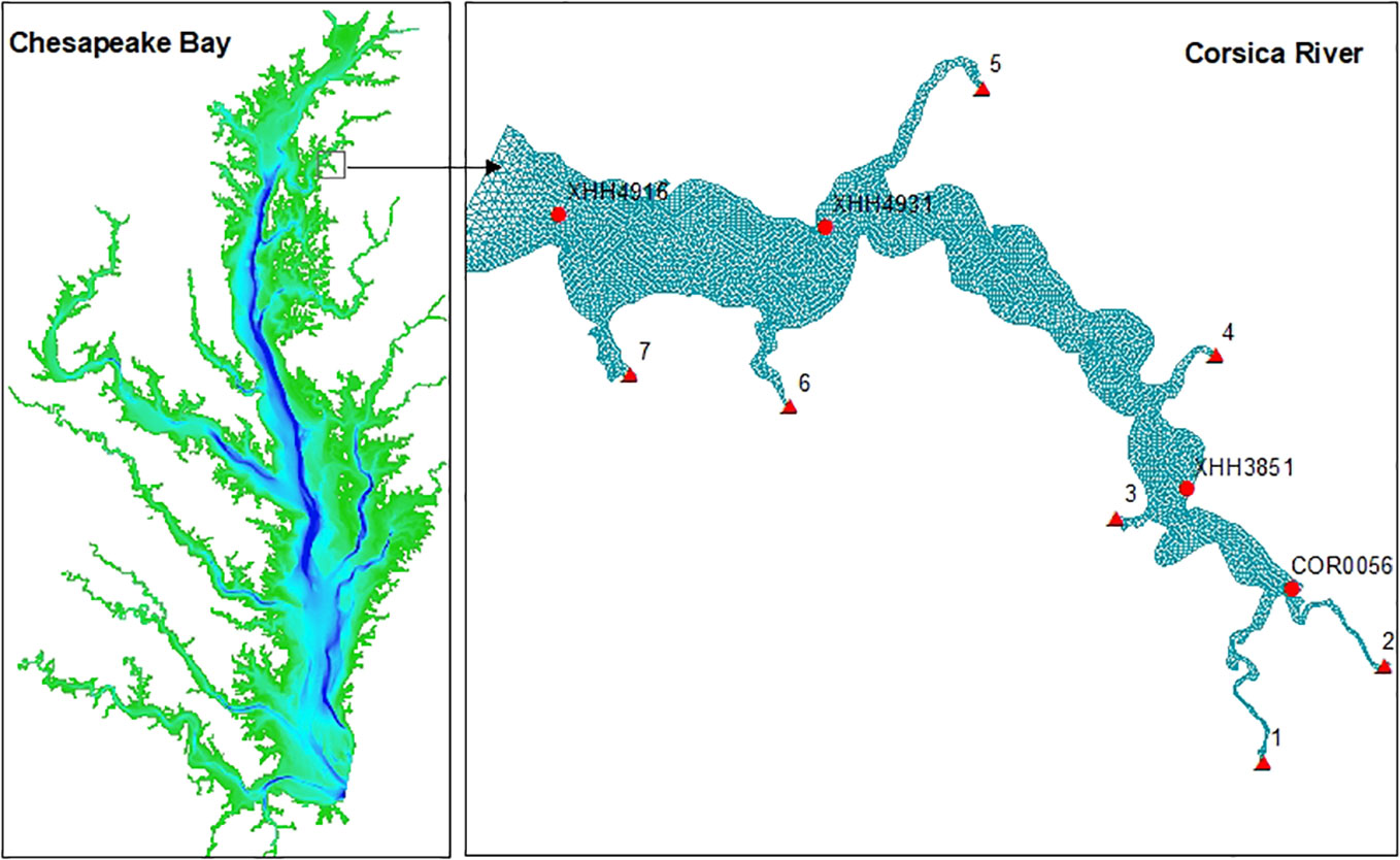
Figure 1 Geographic location of the simulation domain and grid. Background color of the left panel is the Chesapeake Bay bathymetry ranging up to 40 m (blue). Red triangles on the right panel are the seven freshwater discharge locations from the Corsica watershed. Red dots are the four Corsica River stations with cruise-based observation data.

2 Methods

2.1 Models

Detailed description of SCHISM and ICM are available at https://www.schism.wiki. Only a short description is given here. SCHISM employs a flexible unstructured grid with a highly efficient semi-implicit finite-element Eulerian-Lagrangian algorithm to solve the physical (Equations 1 and 2) and transport equations (Equation 3; Zhang et al., 2016):

$\begin{array}{ll}\text{Momentum equation}: \frac{D\mathit{\text{u}}}{Dt}=\frac{\partial }{\partial z}\left(\nu \frac{\partial \mathit{\text{u}}}{\partial z}\right)-g\nabla \eta +F& (1)\end{array}$

$\begin{array}{ll}\text{Continuity equation}:\nabla ·u+\frac{\partial \text{w}}{\partial \text{z}}=0 ; \frac{\partial \eta }{\partial t}+\nabla ·\underset{-h}{\overset{\eta }{\int }}\mathit{\text{u}}dz=0& (2)\end{array}$

$\begin{array}{ll}\text{Transport equation}:\frac{\partial C}{\partial t}+\nabla ·(\mathit{\text{u}}C)=\frac{\partial }{\partial z}(\kappa \frac{\partial C}{\partial z})+F_h& (3)\end{array}$

where ∇ is the differential operator del $\left(\frac{\partial }{\partial x},\frac{\partial }{\partial y}\right)$; η(x,y,t) is the surface elevation; h(x,y) is the bathymetry; u(z,y,z,t) is the horizontal velocity; w is the vertical velocity; F represents other forcing terms such as baroclinic gradient $(-\frac{g}{{\rho }_0}\underset{z}{\overset{\eta }{\int }}\nabla \rho d\zeta )$, horizontal viscosity, Coriolis force, tide, and atmospheric pressure; C is the tracer concentration; ν is the vertical viscosity; κ is vertical eddy diffusivity; and F_h represents the horizontal diffusion and source/sink terms. Flexibility in space and time is the key feature in SCHISM for this study. The unstructured grid ensures that the model fits the complex shoreline in the Corsica River, and the terrain-following vertical grid guarantees fine vertical resolution without bathymetry smoothing. The semi-implicit feature enables the flexibility in the time step and model advancement during the simulation.

ICM has 36 state variables, including three phytoplankton groups; two zooplankton groups; four types of nutrients; labile and refractory dissolved organic carbon (DOC), nitrogen (DON), and phosphorus (DOP); labile (G1), refractory (G2), and inert (G3) particulate organic carbon (POC), nitrogen (PON), and phosphorus (POP); DO; chemical oxygen demand (COD); and five classes of sediments (sand, silt, clay, organic detritus, and total inorganic solids) (Figure 2A). The model structure of ICM is flexible, and the state variables can be turned on or off depending on the interest of each application. In this application, the zooplankton compartments, refractory dissolved organic matters, inert particulate organic matter, silicate, and sediment variables were turned off (Figure 2B). The model has four benthic modules: submerged aquatic vegetation (SAV), tidal wetland, benthic microalgae, and shellfish. In this application, only the benthic microalgae module was activated. Detailed kinetics and parameterization can be found in previous publications (Cerco and Noel, 2004; Tian et al., 2021; Cai et al., 2022). Briefly, the governing equation of phytoplankton (B) is:

Figure 2

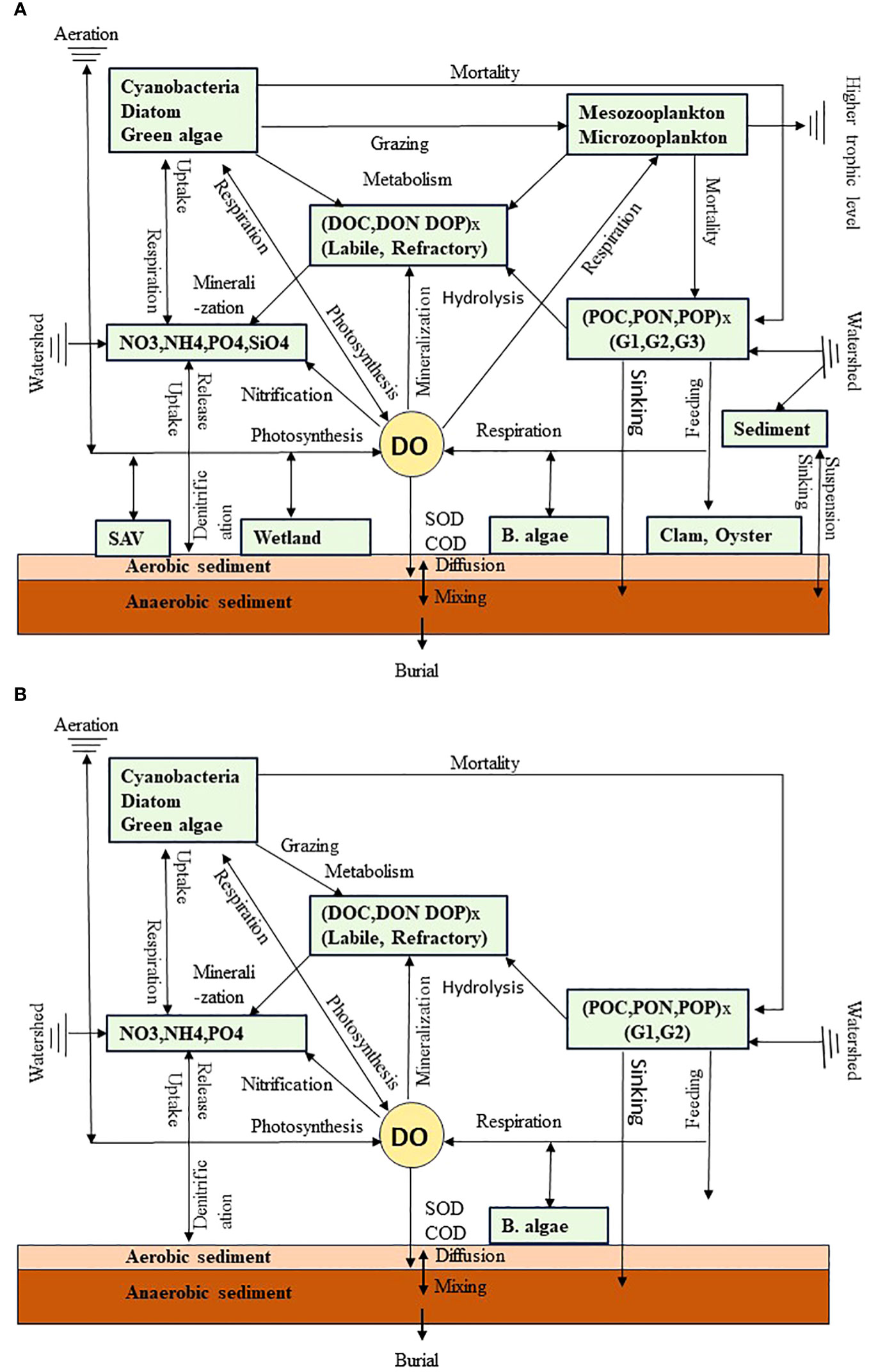
Figure 2 (A) Diagram of the major compartments and energy flows in the water quality model ICM. G1, G2, and G3 are the particulate organic compartment categories based on their reactivity (G1: labile; G2: refractory; and G3: inert). COD is chemical oxygen demand, SOD is sediment oxygen demand, and SAV is submerged aquatic vegetation and sediments including sand, silt, clay, and organic detritus. (B) State variables turned on for this study.

$\begin{array}{ll}\frac{\partial B}{\partial t}=(\text{μ}-{\alpha }_m)·B-{\alpha }_P·B +\nabla ·(\mathit{\text{u}}B)+\nabla ·(\mathit{\text{D}}\nabla B)& (4)\end{array}$

where μ is the phytoplankton growth rate, α_m is the respiration loss term, α_p represents the predation loss and the last two terms are advection and turbulent diffusion, respectively (Equation 4). The phytoplankton growth rate (μ) is controlled by water temperature, photosynthetically active radiation (Jassby and Platt, 1976) and nutrient resource, which is parameterized using the Michaelis-Menten function:

$\begin{array}{ll}\mu ={\text{μ}}_{\text{max}}·e^{-K_{T(1,2)}{(T-T_o)}^2}\frac{I}{\sqrt{I^2+K_I^2}}\min \left(\frac{N}{N+K_N},\frac{P}{P+K_P}\right)& (5)\end{array}$

where µ_max is the maximum growth rate; T_O is the reference temperature where phytoplankton growth rate reaches its maximum, K_T(1,2) is the coefficient determining the temperature control on phytoplankton growth with K_T(1) for temperature < T_O and K_T(2) for temperature > T_O, I is the photosynthetically active radiation (PAR), K_I is the the growth-radiation coefficient, N and P are nitrogen and phosphorus concentrations, and K_N and K_P are the half-saturation constants, respectively (Equation 5).

DO envolves most of the variables and its decription provides an overview of the ICM water quality model. DO is determined by photosynthesis production, respiration consumption, remineralization of DOC, nitrification, chemical oxygen demand (COD), aereation at the sea surface, and sediment oxygen demand (SOD) at the bottom:

$\begin{array}{ll}\frac{\partial DO}{\partial t}=a_{OC}[(1.3-0.3p_{NH})·\mu -{\alpha }_m]·B-a_{ON}·NT-{\alpha }_{DOC}·a_{OC}·\frac{DO}{k_{OC}+DO}·DOC-{\alpha }_{COD·}\frac{DO}{k_{COD}+DO}·COD+\frac{{\alpha }_{air}}{D{Z}_S}(DOs-DO)-\frac{SOD}{D{Z}_B}& (6)\end{array}$

where a_OC is the ratio between oxygen and carbon in phytoplankton and organic matters, p_NH is the preference of ammonium uptake by phytoplankton, a_m is the phytoplankton respiration coefficient, a_ON is the ratio between oxygen and nitrogen in nitrification, NT is nitrification, a_DOC is the DOC remineralization rate, k_OC is the half-saturation constant of DO for DOC remineralization, a_COD is the oxidation rate of COD, k_COD is the half-saturation constant for COD oxidation, DO_s is DO saturation at a given temperature and salinity, DZ_s is the thickness of the surface layer, DZ_B is bottom layer thickness (Equation 6). DO aeration is applied to the surface layer and SOD to the bottom layer. When carbon fixation is based on nitrate uptake, 30% more oxygen is released as compared to ammonium uptake (the 1.3 constant in the first term of Equation 6; Morel, 1983).

The Di Toro (2001) sediment diagenesis model was incorporated in ICM, which simulates fluxes and exchanges at the sediment-water interface. Brady et al. (2013) and Testa et al. (2013). have provided comprehensive description on the diagenesis model application in Chesapeake Bay. Basically, the diagenesis of organic matter deposited to the sediment yields sulfide, methane, and ammonium whose oxidation constitutes the sediment oxygen demand (SOD). Under anaerobic conditions, sulfide and methane can be released directly to the bottom water to support additional oxygen consumption (COD).

The benthic microalga model based on Cerco and Seitzinger (1997) is coupled with SCHISM with an unstructured grid for coastal shallow water systems. The mass balance of benthic microalgae is determined by growth, respiration, and predation loss:

$\begin{array}{ll}\frac{\partial B}{\partial t}=(G-R-P)B& (7)\end{array}$

where B is the benthic microalgal biomass in g C m⁻² and G, R, and P represent the growth, respiration, and predation terms, respectively (Equation 7). Benthic microalgal growth is controlled by light, temperature, and nutrient availability. Benthic microalgal self-shading is parameterized as a function of benthic microalgal biomass and its light attenuation coefficient:

$\begin{array}{ll}{I}_{BA}=I_B{e}^{-k_S}(1-e^{-k_{BI}B})/(k_{BI}B)& (8)\end{array}$

where I_BA is light available to benthic microalgal photosynthesis, I_B is light at the sediment surface, k_S is the sediment solids light attenuation coefficient, and k_BI is benthic microalgal light attenuation for self-shading (Equation 8). The light–growth curve is formulated as the Jassby–Platt function (Jassby and Platt, 1976):

$\begin{array}{ll}f(I)=\frac{I_{BA}}{\sqrt{h_{BI}^2+I_{BA}^2}}& (9)\end{array}$

where the light half saturation h_BI² is related to the ratio of the growth rate [G_Bf(T)] to the initial slope of the light growth curve α_B. f(T) is the temperature influence on benthic microalgal growth and is formulated as an exponential function:

$\begin{array}{ll}f(T)=e^{-kb{(T-T{b}_O)}^2}& (10)\end{array}$

where kb is the exponential coefficient and Tb_O is the reference temperature set at 20°C (Equation 10). Nutrient limitation on benthic microalgae is parameterized with the Michaelis–Menten function:

$\begin{array}{ll}f(N)=\frac{N}{h_N+N}& (11)\end{array}$

where h_N is the half-saturation constant and N is the available nutrient (nitrogen or phosphorus) to benthic microalgae (Equation 11). The available nutrient concentration is computed as the sum of the bottom water concentration and sediment flux divided by the bottom cell thickness. Both respiration and predation loss of benthic microalgae are also formulated as an exponential function:

$\begin{array}{ll}(R,P)=e^{{(}_{\alpha mb},{ }_{\alpha pb}){(T-T{b}_O)}^{}}& (12)\end{array}$

where ${\alpha }_{mb}(\text{or} {\alpha }_{pb})$ is the exponential coefficient for metabolism (or predation) (Equation 12). All the effects of benthic microalgae activities on solute constituents are added to sediment fluxes, including DO photosynthesis production and respiration consumption, nutrient uptake and respiration release, and DOC flux from benthic microalgal metabolism. On the other hand, solids production of benthic microalgae is added to the corresponding sediment components, essentially organic carbon, nitrogen, and phosphorus. Model parameter definition and values are listed in Table 1.

Table 1

Table 1 Parameter definition, values and units (empty cells indicate dimensionless).

The simulation domain covers the entire Corsica River (Figure 1). Grid resolution is approximately 100 m at the river mouth to 20 m near the coastline, with 5,614 cells, 3,159 nodes, and five vertical sigma layers. The simulation time step was set at 120 s. The model was first calibrated with the observation of the entire year 2006 without benthic microalga simulation. This run was used as the benchmark for comparison and called the “control run.” Upon the control run, the benthic microalga simulation was activated and called the “scenario run,” the comparison of which with the control run allowed us to assess the impact of benthic microalgae on DO and nutrient fluxes at the sediment–water interface and primary production, chlorophyll concentration, and DO in the water column, and these for both near-field stations where benthic microalgae grew and far-field stations where benthic microalgae were prohibited by environmental conditions.

2.2 Data

Short and long-wave radiation data were obtained from the Reanalysis V5 (ERA5) of the European Centre for Medium-Range Weather Forecasts (https://www.ecmwf.int/en/forecasts/dataset/ecmwf-reanalysis-v5). Air temperature, wind, precipitation, pressure, and specific humidity data were downloaded from the North American Regional Reanalysis domain (NARR; https://www.ncei.noaa.gov/products/weather-climate-models/north-american-regional). River discharge and nutrient loads were simulated by the Hydrological Simulation Program–FORTRAN (HSPF), calibrated with the USGS River Input Monitoring (RIM) stations of the Chesapeake Bay Program (Shenk et al., 2012; Shenk and Linker, 2013). Daily river discharge and nutrient loads were available at seven loading points in the Corsica River domain for the simulation year (Figure 1). Open boundary conditions were based on the CH3D-ICM simulation in the entire Chesapeake Bay, calibrated against long-term monitoring data for regulatory purposes over the past 30 years (Cerco and Noel, 2019).

Twenty-one discrete sampling events were carried out from April through December by the Department of Natural Resources of Maryland (DNR-MD, USA). Four stations were occupied for measurement of water temperature, salinity, and chlorophyll during each sampling event: the tidal water head station COR005, the upper estuary station XHH3851, the mid-estuary station XHH4931 and lower estuary station XHH4916 (Figure 1). Measurements of sediment oxygen demand (SOD) and sediment-water ammonium fluxes collected during previous projects were also used to validate the diagenesis model simulation (Boynton et al., 2009; Boynton et al., 2018).

2.3 Data analysis

Generalized Additive Model (GAM) was used to identify the major predictors and characterize the nonlinear relationships between the predictors and the dependent variable (Wood, 2004; Wood, 2006; Harding et al., 2016). GAM from the “mgcv” package in R was applied to the simulated timeseries data of benthic microalgae production and DO flux at the sediment water interface with cubic spline (Hastie and Tibshirani, 1986; Murphy et al., 2022). Spectral analysis was performed on the simulated DO flux to identify the major frequencies within the complex variations in the timeseries data (Olson, 1986; Sanford et al., 1990; Fleming et al., 2012). The contribution of each individual frequency is characterized in the periodogram and the variance of each signal is quantified by the spectrum power density, defined as the amplitude power of the signal. Taylor Diagram was used to compare the scenario run with benthic microalgae and the control run without benthic microalgae. Taylor Diagram compares between simulations and observations in terms of correlation coefficients, standard deviations of both simulation and observation and centered root mean squared errors (CRMSE) on the same diagram (Taylor, 2001; Tian et al., 2014). The correlation coefficient between simulation and observation is expressed as the angle from the y axis, the normalized standard deviation (std) of the simulated results (simulation std divided by observation std) is given by the distance from the origin, and the centered root mean squared error of the simulation is measured by the distance between the simulation point and the observation point (see illustration in the “Results” section).

3 Results

3.1 Physical conditions during the simulation year

There was a flushing event in the summer of 2006, with freshwater discharge reaching 27 m³ s^-1 and dissolved inorganic nitrogen (DIN) loads up to 4,200 kg N day^-1 (Figure 3A). River discharge and nutrient loads were also relatively elevated earlier in the year and in the fall. There were two dry periods between the flushing events (Day 60 to 170 and 210 to 240) when river discharge was below 2 m³ s^-1. Air temperature displayed a typical seasonal cycle, up to 36 °C in summer and as low as 0 °C in winter (Figure 3B). In addition to the seasonal cycle, higher frequency variations on the order of weeks to a month was observed. Wind also showed high frequency variability, with frequencies in the order of hours to days (Figure 3B). Stronger wind was observed in winter and fall than in summer. Both seasonal and diel cycles were observed in the timeseries of photosynthetically active radiation (PAR) (Figure 3C). PAR was about 200 W m^-2 during the day in winter and reached up to 450 W m^-2 in summer. On top of the seasonal and diel cycles, cloud coverage interrupted the continuous regular variation, leading to low radiation from time to time regardless of the season.

Figure 3

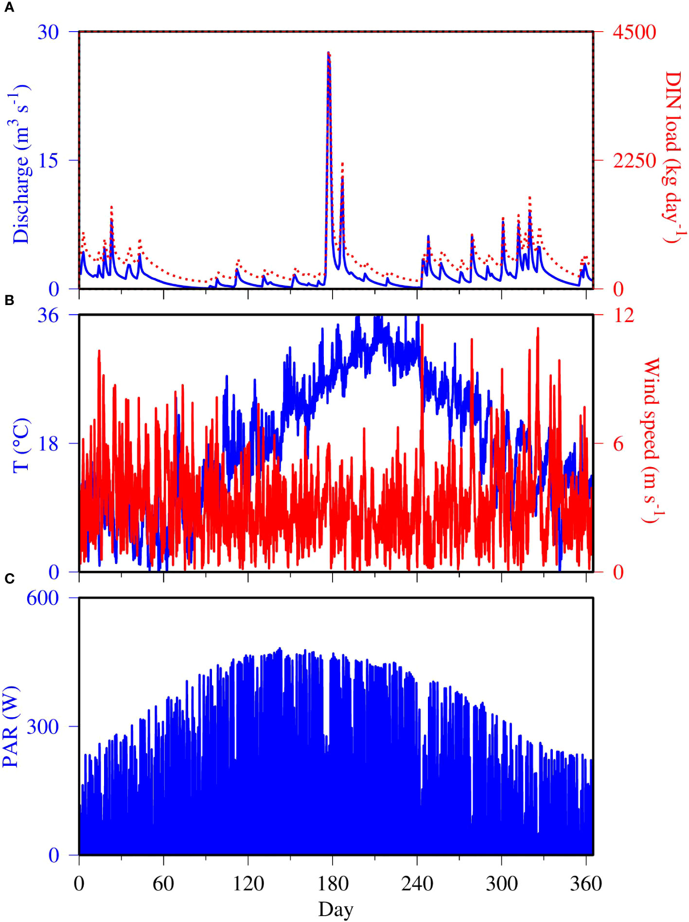
Figure 3 Model physical conditions for the calendar year 2006, including (A) total freshwater discharge (blue line) and DIN load (red dashed line), (B) air temperature (blue line) and wind speed (red line), and (C) PAR (Tian et al., 2022).

3.2 The control run

The control run without benthic microalgae was calibrated with the data and served as a benchmark for comparison with the scenario simulation with benthic microalgae (Figure 4). The model mostly reproduced the observed features in a variety of variables, including temperature (Figures 4A–D), salinity (Figures 4E–H), DO (Figures 4J–L), chlorophyll (Figures 4M–P), SOD (Figures 4Q–T), and ammonium flux from the sediment (Figures 4U–X). Temperature was dominated by the seasonal cycle with low temperature down to 0°C in winter and high temperature up to 35°C in summer. Modeled results compared well with observations, including high-frequency variations on the order of weeks. The major feature in salinity was the freshening event in summer due to high precipitation and freshwater discharge shown in Figure 3. Low salinity was also observed in late winter–early spring due to elevated discharge. The model reproduced these major features in both magnitude and duration. The DO simulation was dominated by a seasonal cycle with high values in spring and fall, low values in summer, and transitional during other periods of the year (Figures 4J–L). On top of the seasonal cycle, the model predicted diel high-frequency variability in DO, resulting from net photosynthetic production during daytime and net respiration consumption during the night. Field observation data were mostly within the range of model prediction. A similar pattern can be observed in the chlorophyll simulation (Figures 4M–P). The model predicted higher chlorophyll concentrations during spring and summer and lower concentrations in the fall and winter. The model also predicted diel frequency variability on top of the seasonal cycle of chlorophyll concentration, which is a phenomenon revealed in shallow water systems by electronic sensor-based continuous monitoring (Shen et al., 2008; Graziano and Jones, 2017; Duvall et al., 2022). The high chlorophyll production in summer was related to the precipitation event that brought high nutrient loads in summer. The chlorophyll data were scattered with large variations. The data tended to support high chlorophyll concentrations in summer at the two upper estuary stations (Figures 4M, N) but showed relatively lower chlorophyll concentrations at the lower estuary stations as compared to the model prediction (Figures 4O,P). These two low estuary stations were closer to the open boundary and more subject to the open boundary conditions. SOD is expressed as negative, implying DO flux from the water column to the sediment (Figures 4Q–T). Larger values were simulated during the summer season than the rest of the year. Variability with frequencies on the order of weeks was simulated in addition to the seasonal cycle. The SOD simulation and observation data were comparable, with data mostly within the range of model variations. Similarly, the ammonium fluxes were also comparable between the data and simulation (Figures 4U–X). Higher values were simulated and observed in summer than during other seasons. Overall, the control run provided a reasonable solution as compared to the observation.

Figure 4

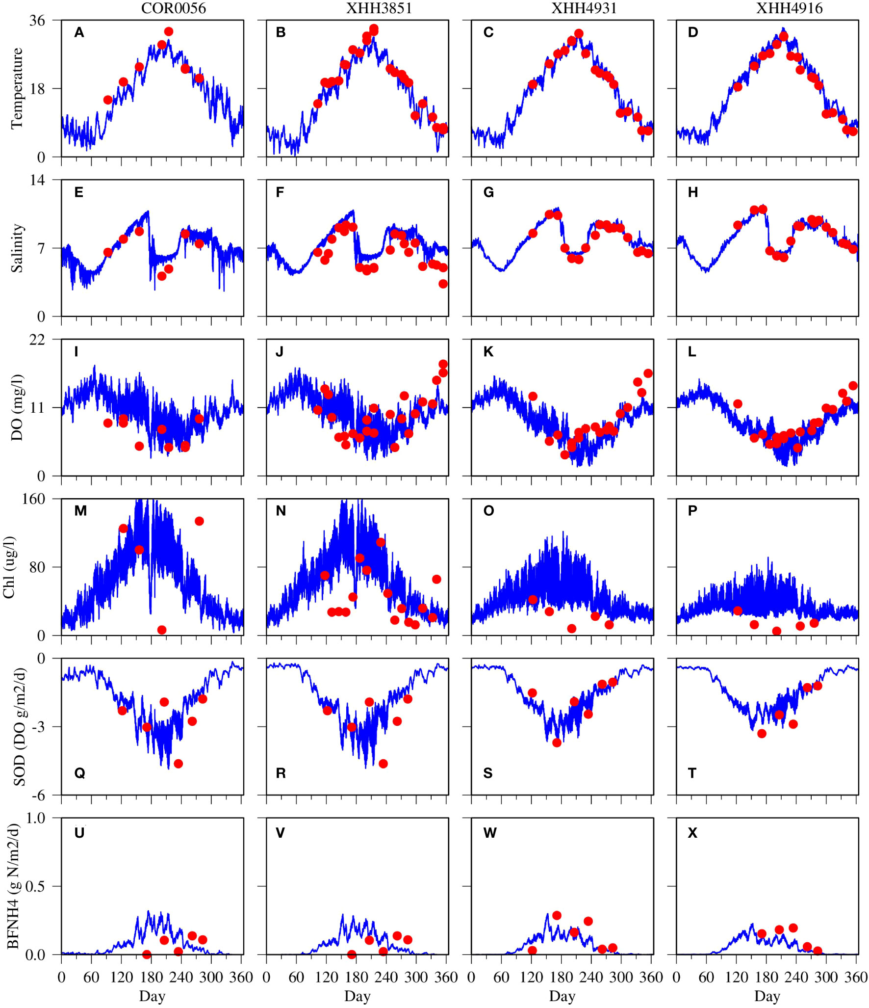
Figure 4 Comparison between model simulations (blue lines) cruise-based, discrete sample data (red dots) at four observation stations for surface water temperature (A-D), salinity (E-H), DO (I-L), chlorophyll (M-P), sediment oxygen demand (Q-T) and ammonium flux at the sediment-water interface (U-X).

3.3 Seasonality and spatial distribution of benthic microalgae

The biomass of benthic microalgae stayed at a relatively elevated level of approximately 5 g C m⁻² early in the year in January and February at the tidal headwater station COR0056 but decreased considerably in March to 3 g C m⁻² (Figure 5). Benthic microalgae bloomed up to 5 g C m⁻² around April, followed by a long period of limited abundance through the summer until October and November when the biomass increased up to 7 g C m⁻² and then decreased to a moderate level of approximately 5 g C m⁻² as at the beginning of the year. The annual average biomass of benthic microalgae was 3.2 g C m⁻², which is within the range of field observation. Gould and Gallagher (1990) reported abundance of benthic diatoms ranging from 2 g C m⁻² to 15 g C m⁻² in the coastal region of Massachusetts Bay. A DNR survey of the Maryland Atlantic coastal regions reported active benthic chlorophyll abundance ranging from 24 mg chlorophyll m⁻² to 52 mg chlorophyll m⁻² (DNR, 2016). Assuming a C:chlorophyll ratio of 50 (19–60; Gould and Gallagher, 1990), the benthic microalgal biomass would range from 1.2 g C m⁻² to 2.6 g C m⁻². Cahoon and Safi (2002) reported active benthic chlorophyll of up to 250 mg m⁻². Benthic microalgal primary production was generally lower during the summer months as compared to that in spring and fall based on remote sensing data and spectral information (Méléder et al., 2020; Jacobs et al., 2021).

Figure 5

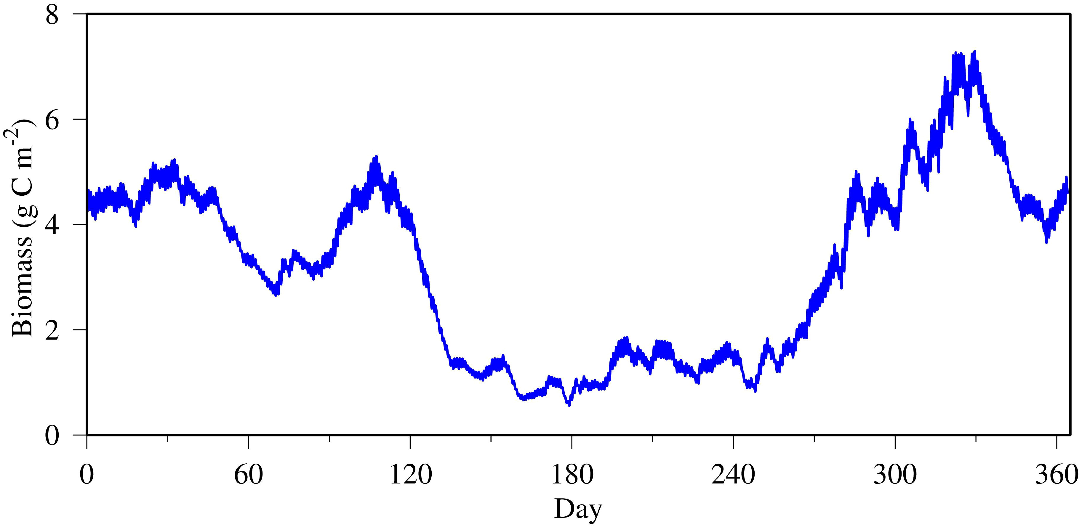
Figure 5 Time series of benthic microalgal biomass simulated at the tidal headwater station COR0056.

Benthic microalgae extended to 2 m deep along the coast, but higher abundance was mostly within the 1-m isobath of bathymetry (Figure 6). Significant abundance of benthic microalgae was simulated in all the tidal headwaters and in most of the coastal regions. Among the four observation stations, only the tidal headwater station COR0056 is located within the benthic microalga zone and all other stations are outside the areas with significant benthic microalga abundance. Consequently, station COR0056 is considered as a near-field station and other stations as far-field stations. Station XHH4931, the mid-estuary station, is in an area where benthic microalgae were particularly scarce so that it is used as an example of far-field stations in the following sections.

Figure 6

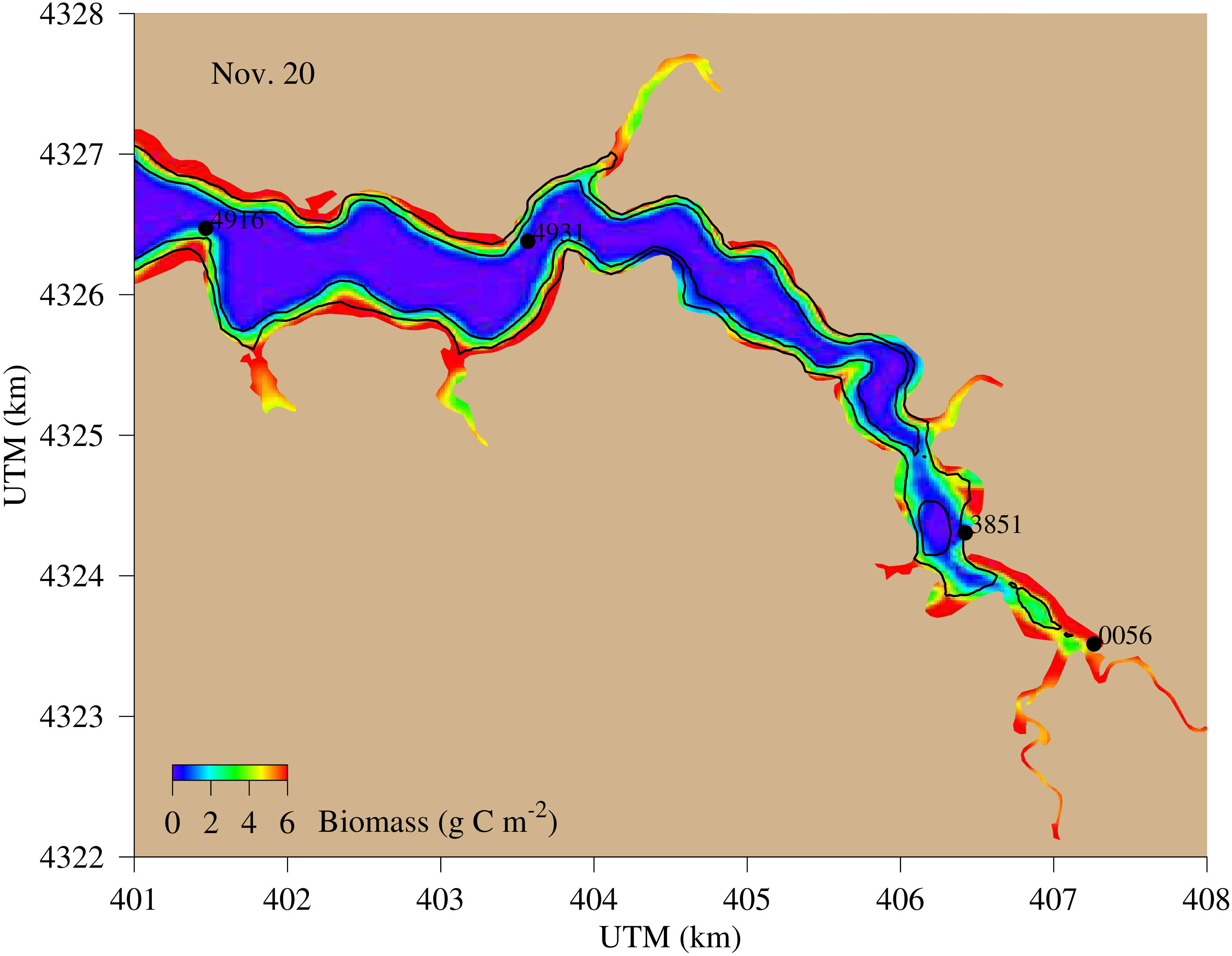
Figure 6 Spatial distribution of simulated benthic microalga abundance (g C m⁻²), an example on Nov. 20. The two black lines are the 1- and 2-m bathymetry, and the black dots are the four observation stations. Only station 0056 is in the benthic microalga productive region.

3.4 Benthic microalgal impact on DO and nutrient flux

High-frequency variability of DO flux with large amplitudes was simulated in the tidal headwater station COR0056 under the influence of benthic microalgae (Figure 7A, green line). The amplitudes reached up to 10 g O m⁻² day⁻¹, and the frequencies were within diel cycles. The control run without benthic microalgae did not generate high-frequency variability (Figure 7A, blue line). The DO flux variability in the simulation without benthic microalgae was mostly within 2 g O m⁻² day⁻¹, and the frequencies were on the order of weeks on top of the seasonal cycle. Both simulations predicted larger DO flux in summer than the rest of the year (negative DO flux indicating DO flux from the water column to the sediment). At the far-field station XHH4931, the model did not predict high-frequency variations in DO flux (Figure 7B). However, the simulation with benthic microalgae (Figure 7B, green line) predicted DO flux significantly larger than the control run without benthic microalgae during the summer season (Figure 7B, blue line). Also, the simulation with benthic microalgae predicted DO flux variations on the order of weeks, whereas these variations were absent in the control run without benthic microalgae.

Figure 7

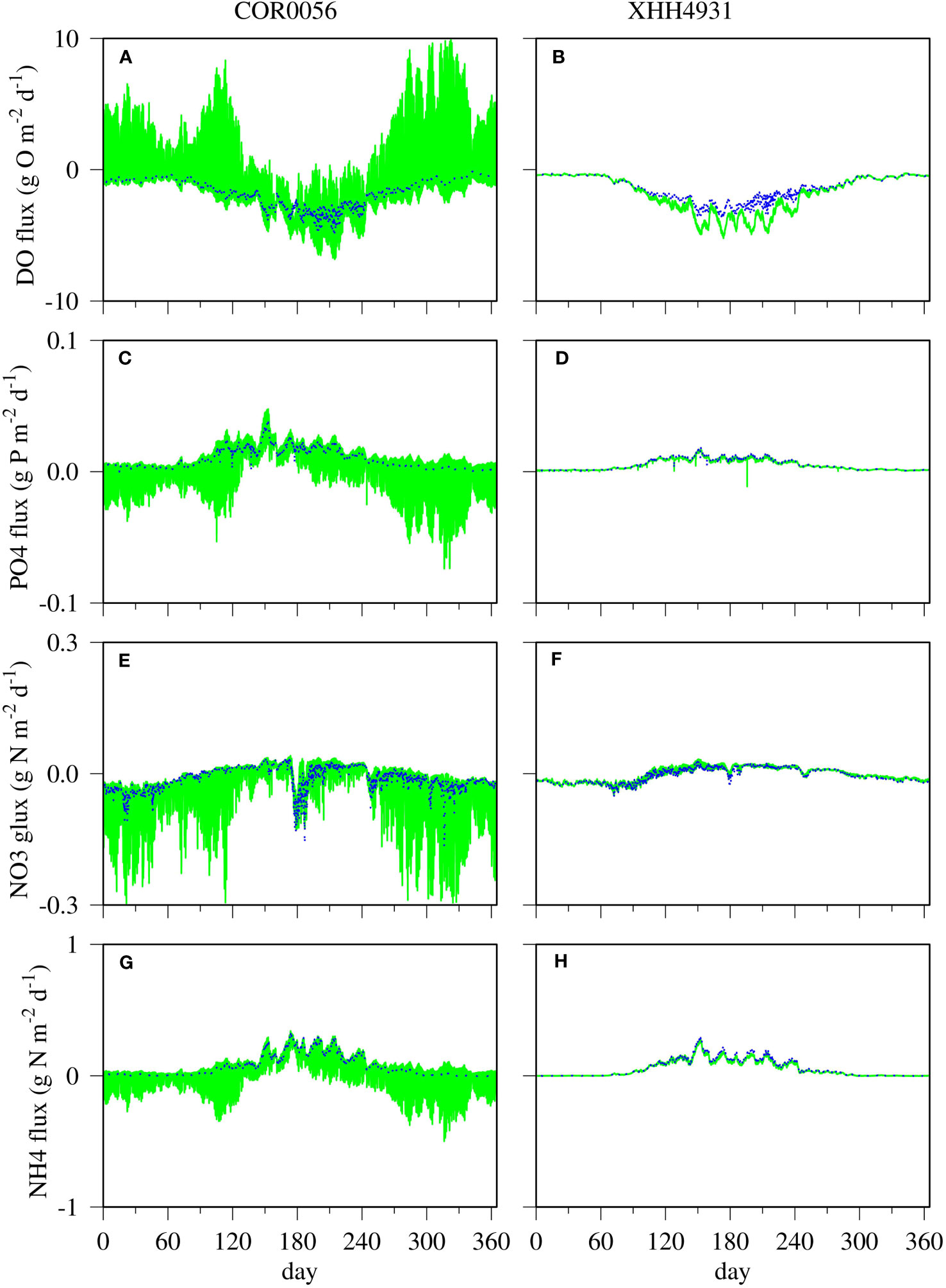
Figure 7 Simulated time-series fluxes at the sediment–water interface at the near-field station COR0056 (left) and far-field station XHH4931 for DO (A, B), phosphate (C, D), nitrate (E, F), and ammonium (G, H). Blue lines are the control run without benthic microalgae, and green lines are the scenario run with benthic microalgae.

Patterns similar to that of the DO flux can be observed in the nutrient flux predictions (Figures 7C–H). High-frequency variability was predicted in the phosphate simulation in the scenario run with benthic microalgae, whereas the control run without benthic microalgae did not generate similar high-frequency variability (Figure 7C). In contrast to the DO flux for which the high-frequency variations were skewed to the positive side (indicating fluxes from the sediment to the water column), the high-frequency variations in phosphate simulation were more skewed to the negative side, indicating phosphate fluxes from the water column to the sediment. In the control run without benthic microalgae (Figure 7C, blue line), the phosphate fluxes were mostly positive, i.e., phosphate release from the sediment to the water column. The seasonal cycle remained in both runs with and without benthic microalgae, with higher phosphate release from sediment in summer than in the rest of the year. However, no significant difference was predicted at the far-field station XHH3941, where the two simulations were practically identical (Figure 7D). Overall, phosphate release from the sediment tended to be lower at the far-field station in the mid-estuary than at the upper estuary.

The high-frequency variability of nitrate fluxes at the sediment–water interface was mostly negative, indicating absorption of nitrate from the water column to the sediment (Figure 7E). Only during summer was the nitrate flux positive, i.e., release from the sediment. It is interesting to note that during a short period of time around day 180, overall negative nitrate fluxes were simulated in both scenarios with and without benthic microalgae. Similar events occurred during other periods of time of the year but with shorter durations and lower amplitudes. The high-frequency variations in the ammonium fluxes were also skewed on the negative side, but significant positive fluxes were simulated during the summer season in the scenario with benthic microalgae (Figure 7G, green line). On the other hand, ammonium fluxes were mostly positive in the control run without benthic microalgae (Figure 7G, blue line). At the far-field station XHH4931, the two simulations were practically identical for nutrient fluxes at the sediment–water interface, meaning that benthic microalgae did not have notable influence on nutrient fluxes at the far-field stations (Figures 7D, F, H).

3.5 Benthic microalgal impact on DO and chlorophyll in the water column

Benthic microalgae had a significant impact on chlorophyll concentration in the water column at the near-field station COR0056 (Figures 8, 9). The Taylor diagram shows an overall improvement in model–data comparison of DO and chlorophyll in the water column (Figure 8). DO simulation in the scenario run with benthic microalgae (red dots and squares) are closer to the data point in the Taylor diagram as compared to the control run without benthic microalgae (blue dots and squares), indicating higher correlation coefficients and smaller root mean square errors with the observation. Most of the correlation coefficients between DO simulation and observation are higher than 0.85, and the centered root mean square errors are smaller than 0.5. The chlorophyll comparison was not as good as the DO simulation, with most of the correlation coefficients lower than 0.85. It is a challenge to compare discrete sampling data to a time series of data with high-frequency variability in which the timing of the variations can considerably degrade the comparison in terms of correlation coefficient and root mean square errors. Moreover, suspension of benthic microalgae can alter the chlorophyll concentration in the water column and affect the model–data comparison that the model does not have the parameterization at the current stage of model development.

Figure 8

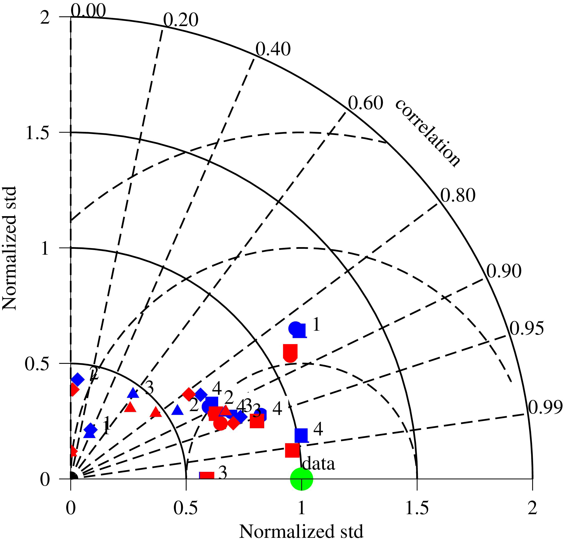
Figure 8 Comparison between the scenario run with benthic microalgae (red) and the control run without benthic microalgae (blue). The green dot is the observation data. The numbers 1–4 represent observation stations from the tidal waterhead to the river mouth, COR0056, XHH3851, XHH4931, and XHH4916, respectively. Dots are surface DO, squares are bottom DO, diamonds are surface chlorophyll, and triangles are bottom chlorophyll. Angles from the y-axis are the correlation coefficients between simulation and observation, distances from the origin are the normalized standard deviation, and the distances between symbols and the data point are the centered root mean square errors. Symbols closer to the data point indicate improvement in model–data comparison. Symbols and numbers are supposed in certain cases.

Figure 9

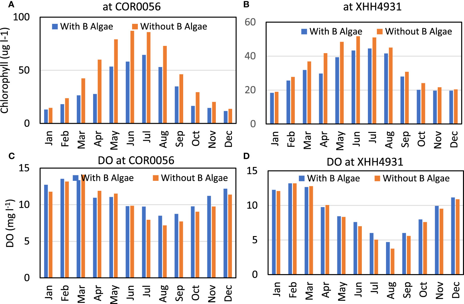
Figure 9 Monthly average concentration of chlorophyll (A, B) and DO (C, D) at the near-field station COR0056 (left) and far-field station XHH4931 (right) simulated in the control run without benthic microalgae (red bars) and the scenario run with benthic microalgae (blue bars).

The monthly average showed that chlorophyll concentration was lower in the scenario run with benthic microalgae than in the control run without benthic microalgae over all the months, but differences were particularly higher in spring and summer than during the rest of the year (Figure 9A). Chlorophyll concentration in the benthic microalga simulation was only 63% of that in the control run in April (38 versus 60 μg L⁻¹). But the two scenarios were more similar in January and December when the difference was within 10%. Chlorophyll concentration was also lower in the scenario run with benthic microalgae than in the control run at the far-field station XHH4931, with differences smaller than that at the near-field station (Figure 9B). Chlorophyll concentration was 81% in the scenario run as compared to the control run in April and at the same level between the two runs in January and December. The annual average chlorophyll concentration in the scenario run with benthic microalgae was 76% of the control run at the near-field station and 90% at the far-field station.

The monthly average DO concentration was slightly higher in the scenario run with benthic microalgae than in the control run during most of the time (Figure 9C). However, in spring from March through June, the monthly average DO concentration was slightly lower in the scenario simulation than in the control run. As the two extrema, the monthly average DO concentration was 19% higher in the scenario simulation than in the control run in July and 4% lower in May. On an annual basis, the monthly average DO concentration was 6% higher in the scenario simulation than in the control run at the near-field station. A similar pattern can be observed at the far-field station, but with reduced differences (Figure 9D). The monthly average DO concentration was slightly higher in the scenario simulation than in the control run during most of the months but slightly lower in March and April. The annual average DO concentration stood at 9.2 mg L⁻¹ in the scenario simulation and 8.8 mg L⁻¹ in the control run, i.e., a difference of 4%.

3.6 Benthic microalgal impact on primary production

Benthic microalgae had a significant impact on the primary production in the water column (Figure 10). At the near-field station COR0056, phytoplankton production was systematically lower in the scenario run with benthic microalgae than in the control run throughout the year (Figure 10A). Phytoplankton production in the scenario run was only 80% of that in the control run in February and 94% in average. Benthic microalgal production was lower in summer than in the rest of the year at the tidal headwater station COR0056, whereas phytoplankton production was the highest in the summer. The correlation coefficient between benthic microalgae and phytoplankton production was −0.86. Benthic microalgal production was higher than the phytoplankton production in November, December, and January but lower than the latter for the rest of the year. On an annual basis, benthic microalgal production was 22% of the phytoplankton production at the near-field station COR0056. Even though phytoplankton production was lower in the scenario run than in the control run, the total primary production with phytoplankton and benthic microalgae combined was higher in the scenario run than in the control run during most of the months. Only in May through July was the total primary production lower in the scenario run with benthic microalgae than in the control run. The annual total primary production was higher by 14% in the scenario run than in the control run at the near-field station.

Figure 10

Figure 10 Primary production at the near-field station COR0056 (A), the far-field station XHH4931 (B), and integrated in the entire estuary (C) Blue is phytoplankton production in the control run without benthic microalgae, red is phytoplankton production in the scenario run with benthic microalgae, gray is benthic microalgal production, and orange is the total primary production with phytoplankton and benthic microalgae combined.

Benthic microalgae did not grow at the far-field station, yet the phytoplankton production in the water column was lower in the scenario run than in the control run (Figure 10B). The difference was the highest in April when the phytoplankton production in the scenario run was only 74% of that in the control run. Annual average phytoplankton production in the scenario simulation with benthic microalgae was lower by 11% than that in the control run without benthic microalgae. The total benthic microalgal production in the entire estuary was 40% of phytoplankton production and 28% of the total primary production with benthic microalgae and phytoplankton production combined. Phytoplankton production integrated in the entire estuary in the scenario run with benthic microalgae was 95% of that in the control run without benthic microalgae, but the total primary production with phytoplankton and benthic microalgae combined was higher by 35% than the total phytoplankton production in the control run.

4 Discussion

4.1 Factors controlling benthic microalgal growth and distribution

The fact that benthic microalgae are mostly limited within the 2-m isobath of water depth results from the controlling factors that impact benthic microalgal growth in deeper waters. Benthic microalgal growth is determined by light, nutrients, and water temperature. During the early months of the year from January through March, temperature was the limiting factor that restricted benthic microalgal growth at both the near-field and far-field stations (Figure 11). Phosphorus started to be limiting in spring, followed by nitrogen limitation in summer at the near-field station COR0056 (Figure 11A). Light availability was also relatively lower in summer but sufficient for benthic microalgae to grow. Phosphorus became more limiting in the fall, followed by temperature restriction in December. At the far-field station, light availability was a limiting factor from spring through fall when the light limiting factor was mostly below 0.2. Consequently, light was the primary controlling factor in determining the spatial distribution of benthic microalgae that was mostly limited to the 2-m isobath of water depth. A non-linear GAM function was fitted between benthic microalgal production and each of the four controlling factors (Figure 12). Light turned out to be the dominant predictor, explaining 65% of the benthic microalgal production variance, far larger than the rest of other factors. Temperature was the second predictor with 5% variance explained, followed by phosphorus, 3%, and nitrogen, 2%. Barranguet et al. (1998) and Blackford (2002) found that nutrient limitation played a minor role in controlling benthic microalgal production, and Bowman et al. (2007) reported that benthic microalgae were often controlled by factors other than nutrient availability. It is noteworthy that none of the relationship between the benthic microalgal production and predictors is linear. Benthic microalgal production reached the peak at a light limitation factor of approximately 0.85 and gradually decreased beyond (Figure 12A). There was a positive relationship between benthic microalgal growth and temperature limitation factor up to 0.6, followed by a decreasing trend (Figure 12B). Limitations from other factors and respiration acceleration are the possible causes for the decreasing trend with temperature. The relationship between benthic microalgal production and nitrogen and phosphorus limitation factors showed similarities with light and temperature in that the benthic microalgal growth rate decreased at the high end of the nutrient limitation factors (Figures 12C, D). The non-linearity between benthic microalgal production and its controlling factors reflects the complexity of coastal shallow water dynamics and the interactions among them.

Figure 11

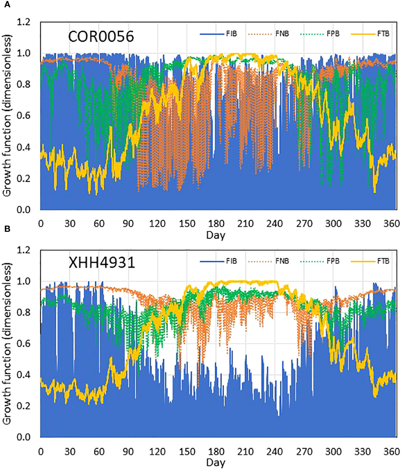
Figure 11 Simulated benthic algal growth limitation factors of light FIB (blue), nitrogen FNB (dashed orange), phosphorus FPB (dashed green), and temperature FTB (yellow) at the near-field station COR0056 (A) and far-field station XHH4931 (B); 1 indicates no limiting effect from a particular resource, and 0 means full limiting effect. Due to the diel cycle, light is always limiting during the night, and its limiting effect is measured by the daytime values, i.e., the upper bound of the blue line.

Figure 12

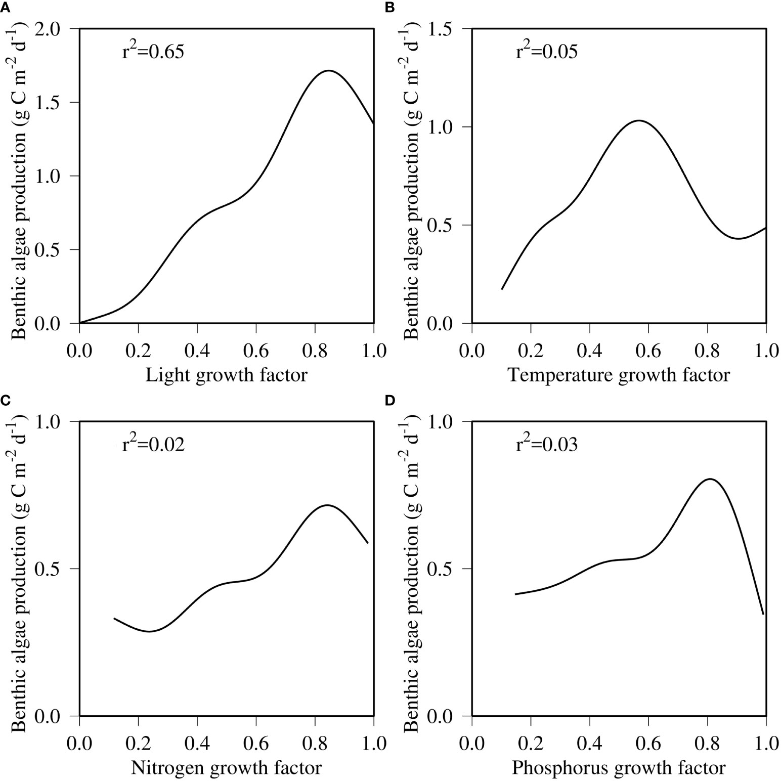
Figure 12 GAM-fitted function between benthic microalgal production and growth factors of light (A), temperature (B), nitrogen (C), and phosphorus (D) at the near-field station COR0056.

4.2 Benthic microalgal impact on high-frequency variability in DO flux

Where present, benthic microalgae resulted in high-frequency variability in DO fluxes. Spectral analysis of the DO flux time-series data of the control run without benthic microalgae did not resolve any high-frequency variability (Figure 13A). An annual cycle with seasonal variation was the only spectral signal resolved in the control run. In the spectral analysis of the DO flux time-series data of the scenario run with benthic microalgae, several high-frequency signals were resolved (Figure 13B). First, the diel signal with a 24-h period constituted the most prominent spectrum in the time series. This was due to benthic microalgal production during the daytime, which produced oxygen that outgassed from the sediment to the water column. Secondly, there was a signal of 12.4 h, which was coherent with the M2 tide frequency. This means that there was a physical signal in the DO flux time series. Tian et al. (2022) reported significant tidal impact on water quality in shallow water systems, and Kwon et al. (2014) observed tidal signals in benthic microalgal production, which ultimately affected DO flux. Tide influences benthic microalgal production mostly through altering environmental conditions, such as temperature, nutrient abundance, water depth, and light availability. Certain species can migrate in response to the tidal phase (Mitbavkar and Anil, 2004). The third signal had a period of 12 h, which happened twice a day. DO flux rapidly increased from sunrise until 10:00 to 11:00 am and then decreased more gradually to sunset, constituting the major component of the diurnal cycle (Figure 13C). Occasionally the peak of DO flux was split, which can be caused by interaction with physics and tide. Unlike the daytime peak, DO flux was mostly unchanged during the night, forming two inflection points at sunrise and sunset. This can be part of the 12-h semidiurnal spectral signal.

Figure 13

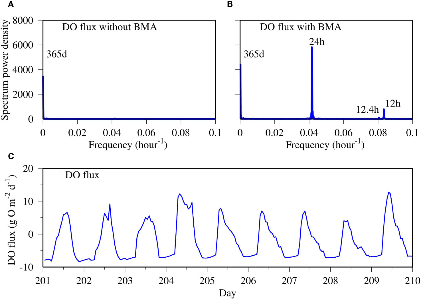
Figure 13 Spectral analysis of DO flux time series predicted in the control run without benthic microalgae (A) and in the scenario run with benthic microalgae (B) and 10-day time-series data of DO flux at the near-field station COR0056 (C).

GAM fitting showed that benthic microalgal production and bottom water temperature explained 99% of the DO flux variance (Figure 14A). Benthic microalgal production alone explained 65% of the DO flux variance, which accounted for most of the high-frequency variability. The relationship between DO flux and benthic microalgal production is practically linear, with high benthic microalgal production leading to high DO flux (Figure 14B). However, GAM fitting showed a non-linear relationship between DO flux and water temperature (Figure 14C). DO flux increased with water temperature until approximately 12°C and then decreased with increasing temperature. High temperature explained most of the extremely low DO flux in summer. Acceleration in mineralization and respiration are behind the negative relationship between DO flux and temperature at the high end.

Figure 14

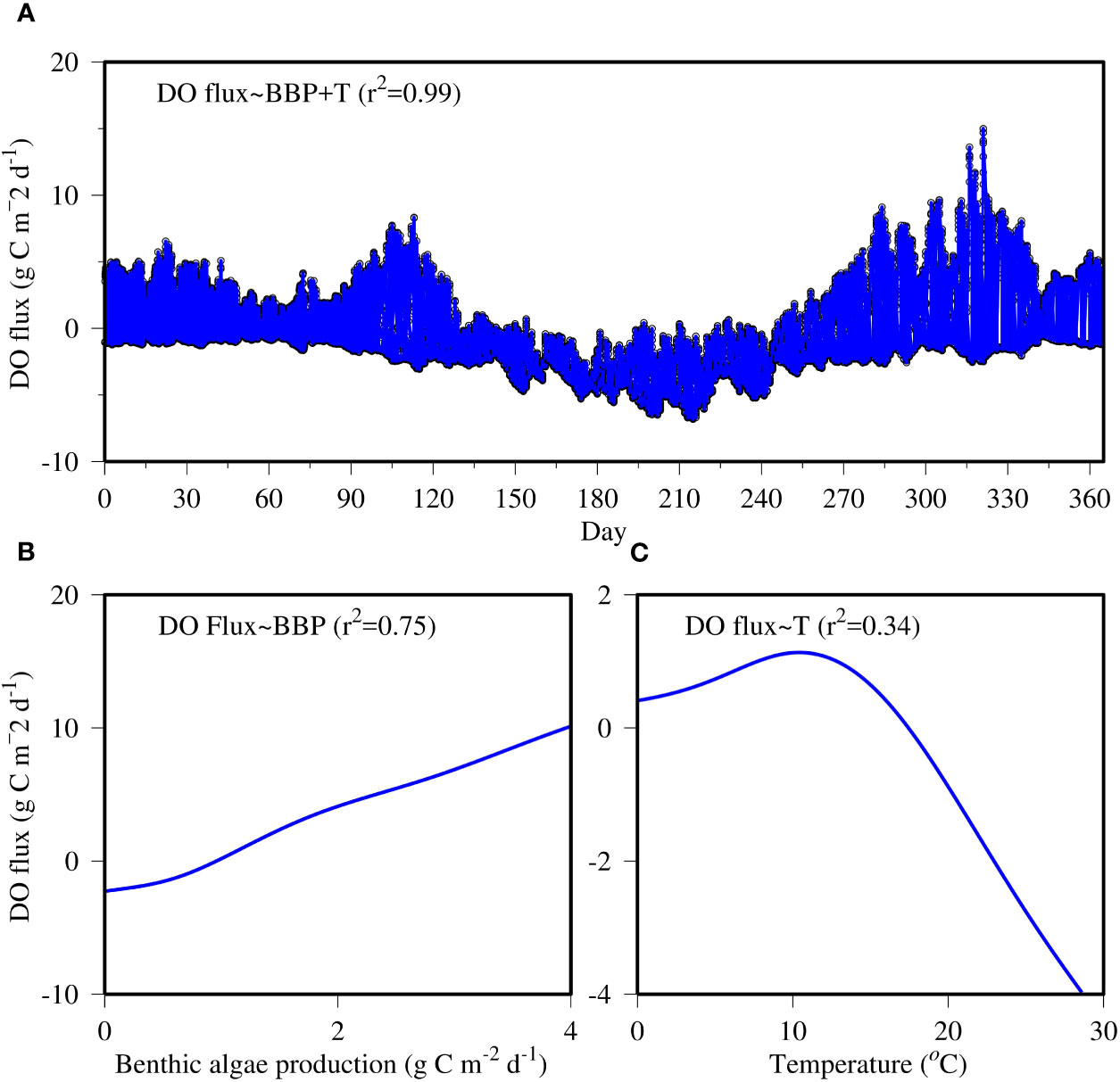
Figure 14 GAM prediction of the DO flux time series at the near-field station COR0056 (A) and fitted functions between DO flux and benthic algal production (B) and water temperature (C). Black circles are the original data of DO flux, and the blue line is the GAM prediction.

4.3 Resource competition between benthic microalgae and phytoplankton in the water column

Interactions between benthic microalgae and phytoplankton constitute a major dynamic in coastal and estuarine shallow water systems (Hope et al., 2020). The model revealed significant resource competition between pelagic phytoplankton and benthic microalgae. Phytoplankton constitute a limiting factor of light reaching the benthic microalgae on the bottom. PAR was high during summer, yet light availability to benthic microalgae was low during the same period. Phytoplankton light attenuation and absorption can considerably reduce light penetration through the water column that sustains benthic microalgal photosynthesis. Yamaguchi et al (2007) found a negative relationship between chlorophyll concentration in the water column and benthic microalgal production, and Darrow (2007) reported the shading effect of phytoplankton on benthic microalgae. On the other hand, benthic microalgae constitute a competitor of phytoplankton nutrient uptake. During the benthic microalga productive season (e.g., April and October), phytoplankton production was significantly reduced, due to the competition of nutrients from benthic microalgae. Overall, nutrient availability to phytoplankton was reduced by one-third over an annual cycle at the near-field station. Laboratory experiments showed a similar phenomenon that benthic microalgae significantly reduced nutrient fluxes from the sediment (Sundback and Graneli, 1988). Field measurement also showed that benthic microalgae sequestered nutrients from being released to the water column during the productive season (Webster et al., 2002).

Shallow water systems account for only approximately 7% of the world ocean surface area but contribute up to 30% of the total primary production (Andersson and Mackenzie, 2004). Shallow waters (≤2 m) occupy 23.7% of the Chesapeake Bay surface area. Being located at the land–ocean interface, shallow water systems are the primary receiver of nutrient loads from watersheds. Understanding benthic microalgal dynamics constitutes a significant element in management decision-making for coastal ecosystem restoration and conservation. The benthic microalga model will be applied to the entire Chesapeake Bay and other tributaries in the coming years. Wave-drive resuspension and climate change can potentially exacerbate benthic algal impact, which are not parameterized in the current microalga model and need further investigation in future applications.

5 Conclusion

The model has reproduced the observed seasonal cycle of a variety of physical and biogeochemical variables, including temperature, salinity, chlorophyll, dissolved oxygen, sediment oxygen demand, ammonium, and phosphorus fluxes at the sediment–water interface. Benthic microalgae were predicted to grow mostly within the 2-m isobath of bathymetry in the Corsica River, and light availability was revealed as the predominant controlling factor in determining the spatial scope of benthic microalgal distribution. The seasonal cycle of benthic microalgal production was also largely determined by light availability, which accounted for 65% of the benthic microalgal production variance. Non-linearity arises from interactions among different controlling factors and between physical and biogeochemical dynamics. Benthic microalgae have considerable impact on DO and nutrient fluxes at the sediment–water interface with high-frequency variability that is dominated by diel, semi-diel, and tidal frequencies. Resource competition occurred between phytoplankton and benthic microalgae. Phytoplankton absorption and shading limit light availability to benthic microalgae and benthic microalgae nutrient uptake reduce nutrient availability to phytoplankton in the water column. However, benthic microalgae represent a net nutrient input from the sediment to the whole system that was not available to phytoplankton production. Benthic microalgal impacts have cascaded through physical dynamics to the far-field stations where phytoplankton production was reduced due to low nutrient availability. Our study shows that benthic microalgae play a significant role in water quality dynamics in shallow water systems, which needs adequate attention in both observation and modeling studies.

Data availability statement

The raw data supporting the conclusions of this article will be made available by the authors, without undue reservation.

Author contributions

RT: Conceptualization, Data curation, Formal analysis, Funding acquisition, Investigation, Methodology, Project administration, Resources, Software, Supervision, Validation, Visualization, Writing – original draft, Writing – review & editing. XC: Conceptualization, Data curation, Formal analysis, Funding acquisition, Investigation, Methodology, Project administration, Resources, Software, Supervision, Validation, Visualization, Writing – original draft, Writing – review & editing. CC: Conceptualization, Data curation, Formal analysis, Investigation, Methodology, Software, Supervision, Validation, Visualization, Writing – original draft, Writing – review & editing. JZ: Conceptualization, Data curation, Formal analysis, Funding acquisition, Investigation, Methodology, Project administration, Resources, Software, Supervision, Validation, Visualization, Writing – original draft, Writing – review & editing. LL: Conceptualization, Data curation, Formal analysis, Funding acquisition, Investigation, Project administration, Resources, Supervision, Validation, Visualization, Writing – original draft, Writing – review & editing.

Funding

The author(s) declare that no financial support was received for the research, authorship, and/or publication of this article.

Acknowledgments

The authors thank the Chesapeake Bay Program and UMCES IAN for providing data and funding (CB-75230480) for this project. Special thanks go to the Chesapeake Bay Program Modeling Team for their enthusiastic help, particularly Gary Shenk, Gopal Bhatt, Jeremy Testa, Damian Brady, Bill Dennison, and Dave Nemazie.

Conflict of interest

The authors declare that the research was conducted in the absence of any commercial or financial relationships that could be construed as a potential conflict of interest.

Publisher’s note

All claims expressed in this article are solely those of the authors and do not necessarily represent those of their affiliated organizations, or those of the publisher, the editors and the reviewers. Any product that may be evaluated in this article, or claim that may be made by its manufacturer, is not guaranteed or endorsed by the publisher.

References

Andersson A. J., Mackenzie F. T. (2004). Shallow-water oceans: a source or sink of atmospheric C0₂? Front. Ecol. Environ. 2, 348–353.

Google Scholar

Barranguet C., Kromkamp J., Peene J. (1998). Factors controlling primary production and photosynthetic characteristics of intertidal microphytobenthos. Mar. Ecol. Prog. Ser. 173, 111–126. doi: 10.3354/meps173117

CrossRef Full Text | Google Scholar

Blackford J. C. (2002). The influence of microphytobenthos on the northern adriatic ecosystem: A modelling study. Estuar. Coast. Shelf Sci. 55, 109–123. doi: 10.1006/ecss.2001.0890

CrossRef Full Text | Google Scholar

Bowman M., Chambers P. A., Schindler D. W. (2007). Constraints on benthic algal response to nutrient addition in oligotrophic mountain rivers. River Res. Appl. 23, 858–876. doi: 10.1002/rra.1025

CrossRef Full Text | Google Scholar

Boynton W. R. (1997). “Chesapeake Bay eutrophication current status, historical trends, nutrient limitation and management actions,” in Proceedings of the Coastal Nutrients Workshop. Artamon, Australia: Australian Water & Wastewater Association Incorporated, 30–31 October 1997. 6–13.

Google Scholar

Boynton W. R., Ceballos M. A. C., Bailey E. M., Hodgkins C. L. S., Humphrey J. L., Testa J. M. (2018). Oxygen and nutrient exchanges at the sediment-water interface: A global synthesis and critique of estuarine and coastal data. Estuar. Coasts 41, 301–333. doi: 10.1007/s12237-017-0275-5

CrossRef Full Text | Google Scholar

Boynton W. R., Testa J. M., Kamp W. M. (2009). “An ecological assessment of the corsica river estuary and watershed scientific advice for future water quality management,” in Maryland department of natural resource, technical report series no. TS-587-09. (Annapolis: Maryland Department of Natural Resource).

Google Scholar

Brady D. C., Testa J. M., Toro D. M. D., Boynton W. R., Kemp W. M. (2013). Sediment flux modeling: calibration and application for coastal systems. Estuar. Coast. Shelf Sci. 117, 107–124. doi: 10.1016/j.ecss.2012.11.003

CrossRef Full Text | Google Scholar

Breitburg D., Levin L. A., Oschlies A., Grégoire M., Chavez F. P., Conley D. J., et al. (2018). Declining oxygen in the global ocean and coastal waters. Science 359, 1–11. doi: 10.1126/science.aam7240

CrossRef Full Text | Google Scholar

Bricker S. B., Longstaff B., W. Dennison W., Jones A., Boicourt K., Wicks C., et al. (2008). Effects of nutrient enrichment in the nation’s estuaries: A decade of change. Harmful Algae 8, 21–32. doi: 10.1016/j.hal.2008.08.028

CrossRef Full Text | Google Scholar

Cahoon L. B. (2006). “Upscaling primary production estimates: Regional and global scale estimates of microphytobenthos production,” in Functionning of microphytobenthos in estuarines. Eds. Kromkamp J., Brouwer J., Blanchard G., Forster R., Créach V. (Amsterdam: Royal Netherlands Academy of Arts and Science), 99–108.

Google Scholar

Cahoon L. B., Safi K. A. (2002). Distribution and biomass of benthic microalgae in Manukau Harbor, New Zealand. N.Z. J. @ Mar. Freshw. Res. 36, 257–266. doi: 10.1080/00288330.2002.9517084

CrossRef Full Text | Google Scholar

Cai X., Zhang Y. J., Shen J., Wang H., Wang Z., Qin Q., et al. (2022). A numerical study of hypoxia in Chesapeake Bay using an unstructured grid model: Validation and sensitivity to bathymetry representation. J. Am. Water Resour. Assoc. 58, 898–921. doi: 10.1111/1752-1688.12887

CrossRef Full Text | Google Scholar

Cerco C. E., Seitzinger P. (1997). Measured and modeled effects of benthic algae on eutrophication in Indian River-Rehoboth Bay, Delaware. Estuaries 20, 231–248. doi: 10.2307/1352733

CrossRef Full Text | Google Scholar

Cerco C. F., Noel M. R. (2004). “The 2002 chesapeake bay eutrophication model,” in EPA 903-R-04-004 (Annapolis, Maryland: U.S. Environmental Protection Agency, Chesapeake Bay Program Office).

Google Scholar

Cerco C. F., Noel M. R. (2019). “2017 chesapeake bay water quality and sediment transport model,” in A report to the US environmental protection agency chesapeake bay program office, 580.

Google Scholar

Dai M., Zhao Y., Chai F., Chen M., Chen N., Chen Y., et al. (2023). Persistent eutrophication and hypoxia in the coastal ocean. Cambridge Prisms: Coast. Futures 1, e19. doi: 10.1017/cft.2023.7

CrossRef Full Text | Google Scholar

Darrow B. P. (2007). “Effects of nutrients from the water column on the growth of benthic microalgae in permeable sediments,” in USF tampa graduate theses and dissertations. (Tampa: University of South Florida). Available at: https://digitalcommons.usf.edu/etd/200.

Google Scholar

Diaz R. J., Rosenberg R. (2008). Spreading dead zones and consequences for marine ecosystems. Science 321, 926–929. doi: 10.1126/science.1156401

PubMed Abstract | CrossRef Full Text | Google Scholar

Di Toro D. M. (2001). Sediment flux modeling (Oxford, U.K.: Wiley), 656.

Google Scholar

DNR (2016). “Ecosystem health assessment of maryland coastal bays: 2007-2013,” in Maryland Department of Natural Resource publication number 12, Resource Assessment Service-772016-609 (Annapolis: Maryland Department of Natural Resource), 334.

Google Scholar

Duvall M. S., Jarvis B. M., Hagy III, J. D., Wan Y. S. (2022). Effects of biophysical processes on diel−cycling hypoxia in a subtropical estuary. Estuar. Coasts 45, 1615–1630. doi: 10.1007/s12237-021-01040-y

CrossRef Full Text | Google Scholar

Fleming S. W., Lavenue A. M., Aly A. H., Adams A. (2012). Practical applications of spectral analysis to hydrologic time series. Hydrol. Process. 16, 565–574. doi: 10.1002/hyp.523

CrossRef Full Text | Google Scholar

Gomez I., Wulff A., Roleda M., Huovinen P., Karsten U., Quartino M., et al. (2010). Light and temperature demands of marine benthic microalgae and seaweeds in polar regions. Botanica Marina 52, 593–608. doi: 10.1515/BOT.2009.073

CrossRef Full Text | Google Scholar

Gould D. M., Gallagher E. D. (1990). Field measurement of specific growth rate, biomass, and primary production of benthic diatoms of Savin Hill Cove. Limnol. Oceanogr. 35, 1757–1770. doi: 10.4319/lo.1990.35.8.1757

CrossRef Full Text | Google Scholar

Graziano A. P., Jones R. C. (2017). Diel and seasonal patterns in continuously monitored water quality at fixed sites in two adjacent embayments of the tidal freshwater Potomac River. Water 9, 624. doi: 10.3390/w9080624

CrossRef Full Text | Google Scholar

Hale S. S., Cicchetti G., Deacutis C. F. (2016). Eutrophication and hypoxia diminish ecosystem functions of benthic communities in a new england estuary. Front. Mar. Sci., 29. doi: 10.3389/fmars.2016.00249

CrossRef Full Text | Google Scholar

Harding L. W. Jr., Gallegos C. L., Perry E. S., Mille W. D., Adolf J. E., Mallonee M. E., et al. (2016). Long-term trends of nutrients and phytoplankton in Chesapeake Bay. Estuar. Coasts 39, 664–681. doi: 10.1007/s12237-015-0023-7

CrossRef Full Text | Google Scholar

Hastie T., Tibshirani R. J. (1986). Generalized additive models (with discussion). Stat. Sci. 1, 297–318. doi: 10.1214/ss/1177013604

CrossRef Full Text | Google Scholar

Hope J. A., Paterson and D. M., Thrush S. F. (2020). The role of microphytobenthos in soft-sediment ecological networks and their contribution to the delivery of multiple ecosystem services. J. Ecol. 108, 815–830. doi: 10.1111/1365-2745.13322

CrossRef Full Text | Google Scholar

Howarth R., Chan F., Conley D. J., Garnier J., Doney S. C., Marino R., et al. (2011). Coupled biogeochemical cycles: Eutrophication and hypoxia in temperate estuaries and coastal marine ecosystems. Front. Ecol. Environ. 9. doi: 10.1890/100008

CrossRef Full Text | Google Scholar

Jacobs P., Pitarch J., Kromkamp J. C., Pilippart C. J. M. (2021). Assessing biomass and primary production of microphytobenthos in depositional coastal systems using spectral information. PloS One 16, e0246012. doi: 10.1371/journal.pone.0246012

PubMed Abstract | CrossRef Full Text | Google Scholar

Jassby A., Platt T. (1976). Mathematical formulation of the relationship between photosynthesis and light for phytoplankton. Limnol Oceanogr. 21, 540–547. doi: 10.4319/lo.1976.21.4.0540

CrossRef Full Text | Google Scholar

Kemp W. M., Boyton W. R., Adolf J. E., Boesch D. F., Boicourt W. C., Brush G., et al. (2005). Eutrophication of Chesapeake Bay: Historical trends and ecological interactions. Mar. Ecol. Prog. Ser. 303, 1–29. doi: 10.3354/meps303001

CrossRef Full Text | Google Scholar

Kwon B. O., Koh C. H., Khim J. S., Park J., Kang S. G. (2014). and hwang, JThe relationship between primary production of microphytobenthos and tidal cycle on the Hwaseong Mudflat, West Coast of Korea. H.J. Coast. Res. 30, 1188–1196. doi: 10.2112/JCOASTRES-D-11-00233.1

CrossRef Full Text | Google Scholar

Longphuirt S. N., Clavier J., Grall J., Chauvaud L., Le Loc’h F., Le Berre I., et al. (2007). Primary production and spatial distribution of subtidal microphytobenthos in a temperate coastal system, the Bay of Brest, France. Estuar Coast. Shelf Sci. 74, 367–380. doi: 10.1016/j.ecss.2007.04.025

CrossRef Full Text | Google Scholar

McGlathery K. J., Reidenbach M. A., D’Odorico P., Fagherazzi S., Pace M. L. (2013). and porter, JNonlinear dynamics and alternative stables states in shallow coastal systems. H.Oceanography 26, 220–231. doi: 10.5670/oceanog.2013.66

CrossRef Full Text | Google Scholar

Méléder V., Savelli R., Barnett A., Polsenaere P., Gernez P., Cugier P., et al. (2020). Mapping the intertidal microphytobenthos gross primary production part I: coupling multispectral remote sensing and physical modeling. Front. Mar. Sci. 7. doi: 10.3389/fmars.2020.00520

CrossRef Full Text | Google Scholar

Mitbavkar S., Anil A. C. (2004). Vertical migratory rhythms of benthic diatoms in a tropical intertidal sand flat: influence of irradiance and tides. Mar. Biol. 145, 9–20. doi: 10.1007/s00227-004-1300-3

CrossRef Full Text | Google Scholar

Morel F. (1983). Principles of aquatic chemistry (New York, NY, USA: John Wiley and Sons).

Google Scholar

Murphy R. R., Keisman J., Harcum J., Karrh R. R., Lane M., Perry E. S., et al. (2022). Nutrient improvements in Chesapeake Bay: Direct effect of load reductions and implications for coastal management. Environ. Sci. Technol. 56, 260–270. doi: 10.1021/acs.est.1c05388

PubMed Abstract | CrossRef Full Text | Google Scholar

Murphy R. R., Kemp W. M., Ball W. P. (2011). Long-term trends in Chesapeake Bay seasonal hypoxia, stratification, and nutrient loading. Estuar. Coasts 34, 1293–1309. doi: 10.1007/s12237-011-9413-7

CrossRef Full Text | Google Scholar

Ni W., Li M., Ross A. C., Najjar R. G. (2019). Large projected decline in dissolved oxygen in a eutrophic estuary due to climate change. JGR Oceans 124, 8271–8289. doi: 10.1029/2019JC015274

CrossRef Full Text | Google Scholar

Olson P. (1986). The spectrum of subtidal variability in Chesapeake Bay Circulation. Estuar. Coast. Shelf Sci. 3, 527–550. doi: 10.1016/0272-7714(86)90008-9

CrossRef Full Text | Google Scholar

Pinckney J. L. (2018). A mini-review of the contribution of benthic microalgae to the ecology of the continental shelf in the south atlantic bight. Estuar. Coast. 41, 2070–2078. doi: 10.1007/s12237-018-0401-z

CrossRef Full Text | Google Scholar

Rabalais N. N., Cai W. J., Carstensen J., Conley D. J., Fry B., Hu X., et al. (2014). Eutrophication-driven deoxygenation in the coastal ocean. Oceanography 27, 172–183. doi: 10.5670/oceanog.2014.21

CrossRef Full Text | Google Scholar

Rizzo W. M., Dailey S. K., Lackey G. J., Christian R. R., Berr B. E., Wetzel R. L. (1996). A metabolism-based trophic index for comparing the ecological values of shallow-water sediment habitats. Estuaries 19, 247–256. doi: 10.2307/1352230

CrossRef Full Text | Google Scholar

Sanford L. P., Sellner K. G., Breitburg D. L. (1990). Covariability of dissolved oxygen with physical processes in the summertime Chesapeake Bay. J. Mar. Res. 48, 567–590. doi: 10.1357/002224090784984713

CrossRef Full Text | Google Scholar

Scavia D., Bertani I., Testa J. M., Bever A. J., Blomquist J. D., Friedrichs M. A. M., et al. (2021). Advancing estuarine ecological forecasts: seasonal hypoxia in Chesapeake Bay. Ecol. Appl. 31, 1–19. doi: 10.1002/eap.2384

CrossRef Full Text | Google Scholar

Semcheski M. R., Egerton T. A., Marshall H. G. (2016). Composition and diversity of intertidal microphytobenthos and phytoplankton in chesapeake bay. Wetlands 36, 483–496. doi: 10.1007/s13157-016-0756-5

CrossRef Full Text | Google Scholar

Serôdio J., Paterson D. M. (2021). “Role of microphytobenthos in the functioning of estuarine and coastal ecosystems,” in Life below water. Eds. Leal Filho W., Azul A. M., Brandli L., Lange Salvia A., Wall T. (Cham: Life Below Water. Encyclopedia of the UN Sustainable Development Goals Springer). doi: 10.1007/978-3-319-71064-8_11-1

CrossRef Full Text | Google Scholar

Shen J., Wang T. P., Herman J., Mason P., Arnold G. L. (2008). Hypoxia in a coastal embayment of the Chesapeake Bay: A model study of oxygen dynamics. Estuar. Coasts. 31, 652–663. doi: 10.1007/s12237-008-9066-3

CrossRef Full Text | Google Scholar

Shenk G. W., Linker L. C. (2013). Development and application of the 2010 chesapeake bay watershed total maximum daily load model. J. Am. Water Resour. Assoc. 49, 1042–1056. doi: 10.1111/jawr.12109

CrossRef Full Text | Google Scholar

Shenk G. W., Wu J., Linker L. C. (2012). Enhanced HSPF model structure for Chesapeake Bay watershed simulation. J. Environ. Eng. 138, 949–957. doi: 10.1061/(ASCE)EE.1943-7870.0000555

CrossRef Full Text | Google Scholar

Sinha E., Michalak A. M., Balaji V. (2017). Eutrophication will increase during the 21st century as a result of precipitation changes. Science 357, 405–408. doi: 10.1126/science.aan2409

PubMed Abstract | CrossRef Full Text | Google Scholar

Su H., Zou R., Zhang X. L., Liang Z. Y., Ye R., Liu Y. (2022). Exploring the type and strength of nonlinearity in water quality responses to nutrient loading reduction in shallow eutrophic water bodies: Insights from a large number of numerical simulations. J. Environ. Manage. 313, 115000. doi: 10.1016/j.jenvman.2022.115000

PubMed Abstract | CrossRef Full Text | Google Scholar

Sundback K., Graneli W. (1988). Influence of microphytobenthos on the nutrient flux between sediment and water: a laboratory study. Mar. Ecol. Prog. Ser. 43, 63–69. doi: 10.3354/meps043063

CrossRef Full Text | Google Scholar

Taylor K. E. (2001). Summarizing multiple aspects of model performance in a single diagram. J. Geophys. Res. 106, 7183–7192. doi: 10.1029/2000JD900719

CrossRef Full Text | Google Scholar

Testa J. M., Brady D. C., Di Toro D. M., Boynton W. R., Cornwell D. C., Kemp M. (2013). Sediment flux modeling: Simulating nitrogen, phosphorus, and silica cycles. Estuar. Coast. Shelf Sci. 131, 245–263. doi: 10.1016/j.ecss.2013.06.014

CrossRef Full Text | Google Scholar

Tian R. (2019). Factors controlling saltwater intrusion across multi-time scale in estuaries: Chester River, Chesapeake Bay. Estuar. Coast. Shelf Sci. 223, 61–73. doi: 10.1016/j.ecss.2019.04.041

CrossRef Full Text | Google Scholar

Tian R. (2020). Factors controlling hypoxia occurrence in estuaries: Chester River, Chesapeake Bay. Water 12, 1–17. doi: 10.3390/w12071961

CrossRef Full Text | Google Scholar

Tian R., Cai. X., Testa J. M., Brady D. C., Cerco C. F., Linker L. C. (2022). Simulation of high-frequency dissolved oxygen dynamics in a shallow estuary, the Corsica River, Chesapeake Bay. Front. Mar. Sci. 9. doi: 10.3389/fmars.2022.1058839

PubMed Abstract | CrossRef Full Text | Google Scholar

Tian R., Cerco C. F., Bhatt G., Linker L. C., Shenk G. W. (2021). Mechanisms controlling climate warming impact on the occurrence of hypoxia in Chesapeake Bay. J. Am. Water Resour. Assoc. 58, 855–875. doi: 10.1111/1752-1688.12907

CrossRef Full Text | Google Scholar

Tian R., Chen C., Qi J., Ji R., Beardsley R. C., Davis C. (2014). Model study of nutrient and phytoplankton dynamics in the Gulf of Maine: patterns and drivers for seasonal and interannual variability. ICES J. Mar. Sci. 72, 388–402. doi: 10.1093/icesjms/fsu090

CrossRef Full Text | Google Scholar

Underwood G. J. C. (2005). Microalgal (microphytobenthic) biofilms in shallow coastal waters: how important are species? Proc. Calif. Acad. Sci. 56, 162–169.

Google Scholar

Underwood G. J. C., Kromkamp J. (1999). Primary production by phytoplankton and microphytobenthos in estuaries. Adv. Ecol. Res. 29, 92–153. doi: 10.1016/S0065-2504(08)60192-0

CrossRef Full Text | Google Scholar

Varela M., Penas E. (1985). Primary production of benthic microalgae in an intertidal sand flat of the Ria de Arosa, NW Spain. Mar. Ecol. Prog. Ser. 25, 111–119. doi: 10.3354/meps025111

CrossRef Full Text | Google Scholar

Wåhlström I., Höglund A., Almroth-Rosell E., MacKenzie B. R., Gröger M., Eilola K., et al. (2020). Combined climate change and nutrient load impacts on future habitats and eutrophication indicators in a eutrophic coastal sea. Limnol. Oceanogr. 65, 2170–2187. doi: 10.1002/lno.11446

CrossRef Full Text | Google Scholar

Wazniak C. (2016). “Benthic microalgae in the maryland coastal bays,” in Maryland’s coastal bays: ecosystem health assessment, maryland DNR report(Annapolis), 141–248.

Google Scholar

Webster I. T., Ford P. W., Hodgson B. (2002). Microphytobenthos contribution to nutrient-phytoplankton dynamics in a shallow coastal lagoon. Estuaries 25, 540–551. doi: 10.1007/BF02804889

CrossRef Full Text | Google Scholar

Wood S. N. (2004). Stable and efficient multiple smoothing parameter estimation for generalized additive models. J. Am. Stat. Assoc. 99, 673–686. doi: 10.1198/016214504000000980

CrossRef Full Text | Google Scholar

Wood S. N. (2006). Generalized additive models (An introduction with R) (Boca Raton: Chapman & Hall CRC), 392.

Google Scholar

Xia M., Craig P. M., Schaeffer B., Stoddard A., Liu Z., Peng M., et al. (2010). Influence of physical forcing on bottom-water dissolved oxygen within Caloosahatchee River Estuary, Florida. J. Environ. Eng. 136, 1032–1044. doi: 10.1061/(ASCE)EE.1943-7870.0000239

CrossRef Full Text | Google Scholar

Xia M., Craig P. M., Wallen C. M., Stoddard A., Mandrup-Poulsen J., Peng M. (2011). Numerical simulation of salinity and dissolved oxygen at Perdido Bay and adjacent coastal ocean. J. Coast. Res. 27, 73–86. doi: 10.2112/JCOASTRES-D-09-00044.1

CrossRef Full Text | Google Scholar

Xia M., Jiang L. (2015). Influence of wind and river discharge on the hypoxia in a shallow bay. Ocean Dyn. 65, 665–678. doi: 10.1007/s10236-015-0826-x

CrossRef Full Text | Google Scholar

Xiao Z., Yang Z., Wang T., Sun N., Wigmosta M., Judi D. (2021). Characterizing the non-linear interactions between tide, storm surge, and river flow in the Delaware Bay Estuary, United States. Front. Mar. Sci. 8. doi: 10.3389/fmars.2021.715557

CrossRef Full Text | Google Scholar

Yamaguchi H., Montani S., Tsutsumi H., Hamada K., Ueda N., Tada K. (2007). Dynamics of microphytobenthic biomass in a coastal area of western Seto Inland Sea, Japan. Estuar. Coast. Shelf Sci. 75, 423–432. doi: 10.1016/j.ecss.2007.05.025

CrossRef Full Text | Google Scholar

Zhang Y. L., Ye F., Stanev E. V., Grashorn S. (2016). Seamless cross-scale modeling with SCHISM. Ocean Model. 102, 64–81. doi: 10.1016/j.oceanmod.2016.05.002

CrossRef Full Text | Google Scholar