Neural network models for seabed stability: a deep learning approach to wave-induced pore pressure prediction

1 Introduction

The phenomenon of wave cyclic loading in submarine sediments can result in pore pressure accumulation, leading to various geohazards such as seabed liquefaction (Wang and Liu, 2016), submarine landslides (Wang et al., 2020), sediment failure (Zhang et al., 2023), sediment rapid erosion (Jia et al., 2014), and instability of structures such like submarine pipelines (Ye and He, 2021) and marine platforms. Accurate prediction of long-term wave-induced pore pressure is crucial for assessing the mechanical state of submarine sediments and ensuring seabed stability, thereby aiding in marine disaster prevention and mitigation.

In recent decades, researchers have made efforts to understand the realistic response of the seafloor through in situ monitoring (Du et al., 2021; Hu et al., 2023), providing valuable data for subsequent physical simulation tests and numerical modeling. Flume tests have also been employed to study the wave-induced pore pressure response and liquefaction, enabling the investigation of liquefaction processes and influencing factors, as well as the sediment resuspension phenomena and redeposition after liquefaction (Jia et al., 2014; Xu et al., 2016). Additionally, finite element numerical simulations have been used to explore the pore pressure response under wave action, aligning well with results from water flume tests and analytical solutions (Ye et al., 2015). In recent years, there has been significant research focus on the following directions in numerical simulation: multi-layer seabed liquefaction calculations (Liu et al., 2023), slope stability under wave actions (Wang et al., 2020), and the stability of marine facilities, such as caisson (Duan et al., 2023), foundation (He and Ye, 2023a; He and Ye, 2023b), and wind turbines (Chang and Jeng, 2014).

However, previous numerical simulation studies relied on statistical and simplified ocean wave conditions (Jia et al., 2014; Ye et al., 2015; Ye et al., 2017; Wang et al., 2020), limiting their ability to simulate wave-induced pore pressure response under specific scenarios and hindering the prediction of pore pressure based on actual ocean wave data. Traditional numerical simulation methods are inadequate for capturing the long-term wave-induced pore pressure response in the ocean and fail to represent real oceanic conditions. Developing a method capable of predicting long-term pore pressure based on real wave data would enhance our understanding of oceanic pore pressure variations and contribute to the effective prevention of marine geohazards.

In recent years, artificial intelligence (AI) technology has been increasingly applied to various geological problems due to its ability to effectively tackle nonlinear problems, such as earthquake prediction (Laurenti et al., 2022), landslide hazard assessment (Collico et al., 2020; Ji et al., 2020; Jones et al., 2021; Du et al., 2022), meteorological and climate forecasting (Balogun et al., 2021; Zennaro et al., 2021), and geophysical data interpretation (Lawson et al., 2017; Maxwell et al., 2019; Politikos et al., 2021; Du et al., 2023). Scholars have made progress in the field of geological time series prediction using AI techniques, for example, wave height prediction (Gao et al., 2021), pore pressure prediction in landslides (Orland et al., 2020; Wei et al., 2021), and prediction of landslide displacement (Yang et al., 2019). The successful application of AI in these research areas demonstrates its potential to address time series prediction problems in the field of geology. However, there is still a lack of research on modeling and prediction using real-time wave-induced pore pressure data obtained from in-situ monitoring in marine environments.

Therefore, the objective of this study is to investigate the feasibility of using three different recurrent neural network (RNN) models to predict the response of wave-induced pore pressure in marine environments, utilizing long-term time series data obtained from in-situ monitoring. The study aims to compare the performance of different RNN models, at different seabed depths, as well as the impact of model parameters and input parameters on prediction accuracy. The findings of this research can provide guidance and recommendations for the development of wave-induced liquefaction early warning systems. Furthermore, this work can serve as a valuable reference for the application of RNNs in other time series problems within the field of geology.

2 Data and method

2.1 Data description

We utilized a supervised deep-learning model to establish the relationship between input parameters and output results. The input parameters considered in this study include water depth (D), effective wave height (H_1/3), effective wave height period (T_1/3), maximum wave height (H_max), maximum wave height period (T_max), wind speed (WS), and wind direction (WD), while the output result is the wave-induced pore water pressure. All the data were obtained from in-situ observations conducted by the First Institute of Oceanography, MNR between February 18, 2015, and April 21, 2015 in the Yellow River Estuary, China (Du et al., 2021; Song et al., 2022).

The in-situ pore water pressure (PWP) data was obtained using a self-developed pore pressure monitoring equipment during the period of maximum wind and wave activity of the year. This dataset includes PWP data measured at depths of 0.5m, 1.5m, 2.5m, and 3.5m below the seabed surface. PWP was measured at a frequency of 0.5 Hz for a duration of 3 minutes every half-hour. We processed the data using interpolation and averaging methods, resulting in continuous pore pressure data with an acquisition frequency of one-half hour, covering a period of over 1500 hours.

During the observation period when the PWP data was collected, we simultaneously gathered data on water depth using a turbidimeter (OBS-3A), wave dynamics using wave-tide instruments (RBR solo D Wave, TGR-2050), and wind conditions with an anemometer (Du et al., 2021). The coordinates for the pore pressure, water depth, and wave data collection site are 118.86°E, 38.20N. Wind speed and wind direction data were sourced using a R.MYOUNG 05106 marine type wind anemometer from an offshore drilling rig situated approximately 300 m northwest of the pore pressure monitoring location. The dataset of these geological parameters covers the entire period of pore pressure monitoring, with a data collection frequency of one record every half hour.

The dataset used for calculations is a two-dimensional array consisting of 3025 rows and 11 columns. The first seven columns represent the calculated parameters, which include water depth, effective wave height, effective wave height period, maximum wave height, maximum wave height period, wind speed, and wind direction. The last four columns represent the pore pressure sensor values at four different depths.

2.2 Correlation analysis of input parameters and pore pressure

We generated a heatmap through correlation analysis using 3000 data sets of the nine parameters mentioned above, as depicted in Figure 1. The heatmap allowed us to explore the correlation between eight input parameters: pore pressure at time t-1 (P_t-1), water depth (D), effective wave height (H_1/3), effective wave period (T_1/3), maximum wave height (H_max), maximum wave period (T_max), wind direction (WD), wind speed (WS), and the output parameter, pore pressure at time t (P_t). When considering the significant influencing factors of pore pressure, it is essential to consider both statistically significant factors and geologically meaningful factors comprehensively.

FIGURE 1

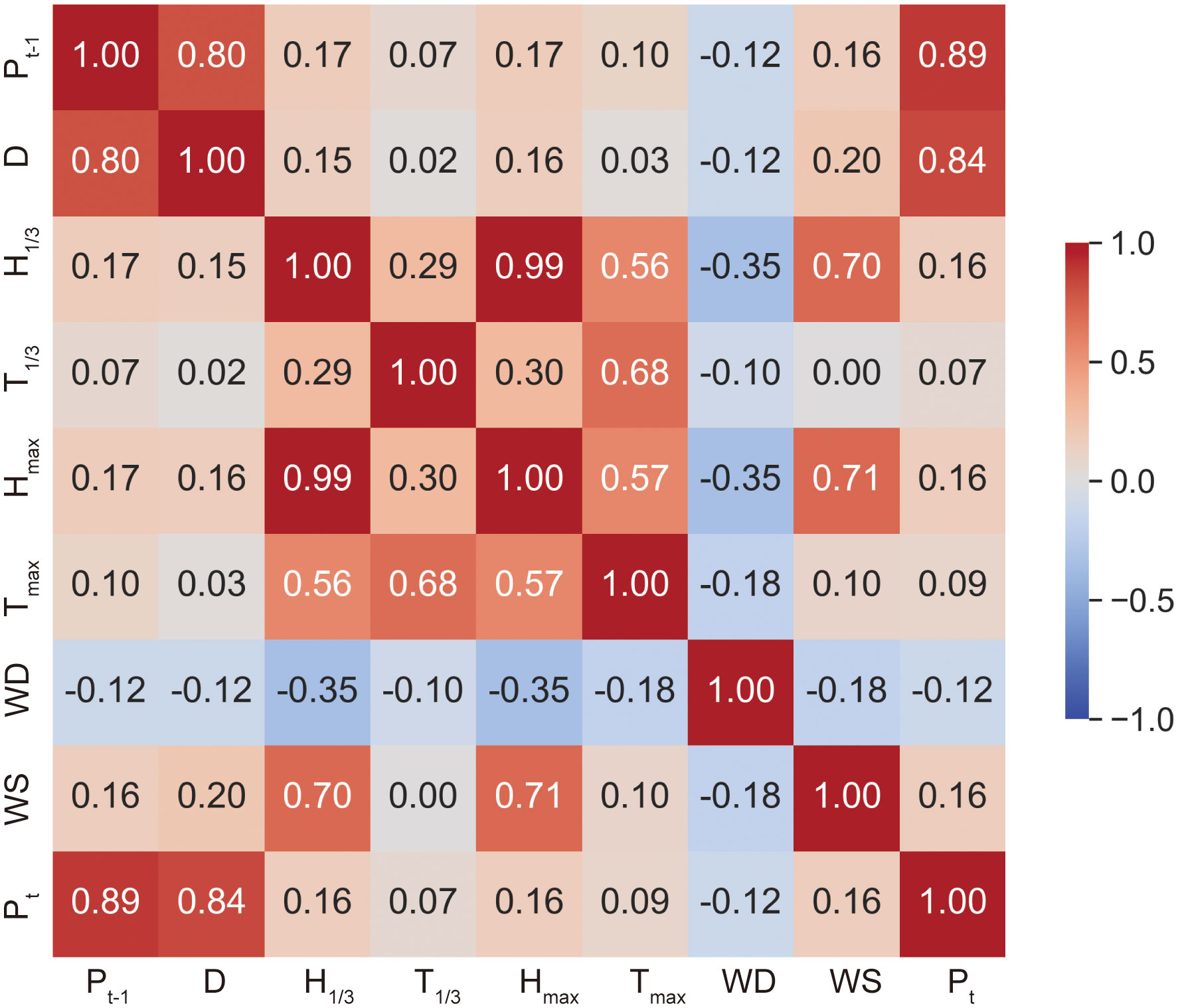
Figure 1 Correlation analysis on pore pressure and geological environment factors. Where the map contains pore pressure at time t-1 (P_t-1), water depth (D), effective wave height (H_1/3), effective wave period (T_1/3), maximum wave height (H_max), maximum wave period (T_max), wind direction (WD), wind speed (WS), and pore pressure at time t (P_t).

Our analysis revealed a strong positive correlation between the input parameters P_t-1 and D with P_t, indicating their significant influence on pore pressure prediction. Thus, P_t-1 and D are considered the most important parameters in determining P_t.

In contrast, the parameters H_1/3, H_max, WD, and WS demonstrated relatively weaker correlations with P_t. While wave height, wind speed, and wind direction are important factors influencing pore pressure variation in submarine sediments, the wave period has minimal impact due to its limited variability and periodicity. Therefore, it can be disregarded. Although wave height, wind speed, and wind direction are slightly less influential compared to pore pressure and water depth at t-1, including them provides additional geological environmental factors that enrich the geological information for pore pressure prediction, bringing the analysis closer to natural environmental influences.

However, the parameters T_1/3 and T_max exhibited the weakest correlations with P_t, with correlation coefficients one to two orders of magnitude smaller than the other parameters. Consequently, it may be reasonable to exclude T_1/3 and T_max from practical calculations or analyses. Based on these results, we recommend prioritizing the inclusion of P_t-1 and D in further analysis or modelling efforts due to their strong positive correlation with P_t. The inclusion or exclusion of H_1/3, H_max, WD, and WS should be carefully considered based on specific analysis goals and requirements.

When selecting input parameters for modelling, it is imperative to consider three crucial aspects: mathematical or statistical relevance, geological significance, and the feasibility of data acquisition.

Firstly, from a mathematical standpoint, pore pressure at the previous time step (P_t-1) and water depth (D) exhibited significant positive correlation with the target variable, pore pressure at the current time step (P_t). Therefore, they are naturally the first choices as input variables. However, relying solely on these two parameters could overlook the influence of wave action, which is a significant contributor to seabed pore pressure variations.

Secondly, the geological significance mandates the inclusion of wave-related parameters. Wave action is a critical factor in seabed pore pressure fluctuations and cannot be disregarded. Therefore, wave-related parameters like effective wave height (H_1/3) and maximum wave height (H_max) are also considered as inputs to bring the model closer to realistic conditions.

Additionally, wind speed (WS) is relatively easily obtainable variables. As evident from Figure 1, wind speed shows a robust correlation with wave action. This raises an interesting question about the feasibility of using wind speed as a proxy for wave parameters, which is a subject worth exploring in our study.

2.3 Applied RNN models

In this study, we employ three types of Recurrent Neural Networks (RNN) (Rumelhart et al., 1986) to model and predict wave-induced pore pressure: the standard RNN, Long Short-Term Memory (LSTM) (Hochreiter and Schmidhuber, 1997), and Gated Recurrent Unit (GRU) (Cho et al., 2014). Here, we provide a brief introduction to the basic forms of RNN and GRU, along with their respective formulas.

2.3.1 Standard RNN model

RNN is a class of artificial neural network designed for processing sequential data (Figure 2A). RNN has demonstrated its effectiveness in various tasks, such as time series prediction, natural language processing, and speech recognition. In RNN, the hidden layers possess a looping mechanism that allows the network to maintain information from previous time steps, enabling it to capture temporal dependencies in the input data. This feature makes RNN suitable for analysing time-dependent phenomena in marine geology, such as predicting sediment transport patterns and wave-induced pore water pressure variation. However, it is noteworthy that the standard RNN model has some limitations, notably the vanishing gradient problem, which can make it challenging for the network to learn long-term dependencies in the data. That is, when performing pore pressure prediction for long time series, the conventional RNN will be less accurate.

FIGURE 2

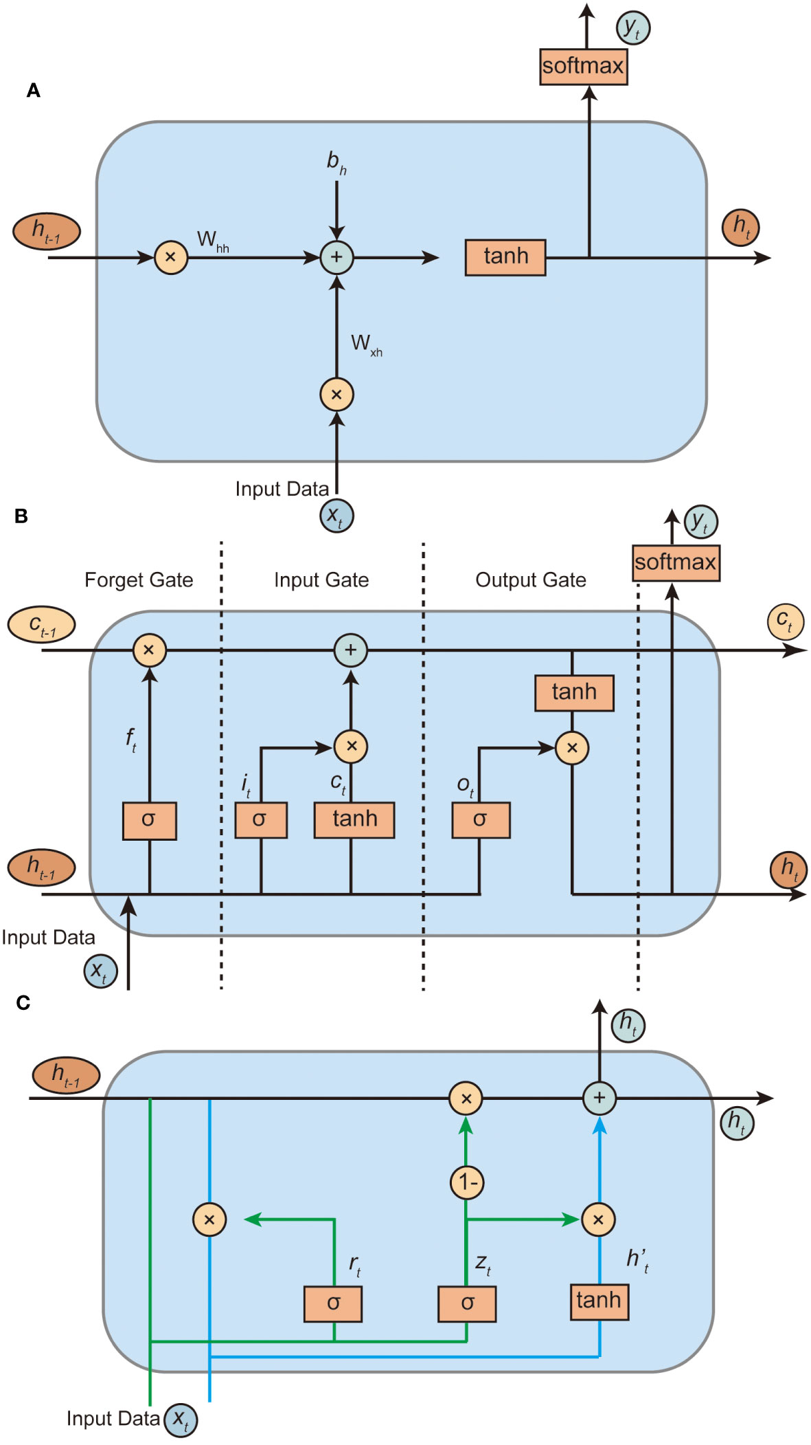
Figure 2 Structure of Standard RNN (A), LSTM (B) and GRU (C) cells.

The standard RNN is composed of an input layer, a hidden layer with a recurrent loop, and an output layer. The key feature of RNN is the ability to retain information from previous time steps in the hidden layer, which enables the model to capture temporal dependencies in the input data. The updated equations for a standard RNN are as follows:

$\begin{array}{ll}{h}_t=\text{tanh }(W_{xh}·x_t+W_{hh}·h_{t-1}+b_h)& (1)\end{array}$

$\begin{array}{ll}{y}_t=softmax(W_{hy}·h_t+b_y)& (2)\end{array}$

where $h$_t $$ is the hidden state at time step t; $x$_t is the input at time step t; $y$_t is the output at time step t; $W$_xh $, W$_hh, and $W$_hy are the weight matrices; $b$_h and $b_y$are the bias terms; tanh is the hyperbolic tangent activation function.

2.3.2 LSTM model

LSTM is a type of Recurrent Neural Network that has been widely used for sequence modeling problems (Figure 2B). Unlike traditional RNN, LSTM is designed to mitigate the vanishing gradients problem and to preserve information across long sequences, by introducing an additional memory cell that can store information for an extended period of time (Gers et al., 2000). LSTM is particularly useful for processing sequences of data with dependencies between time steps, such as time series, speech recognition, and natural language processing tasks.

An LSTM unit is comprised of three gates, which control the flow of information into and out of the memory cell. These gates are the input gate, the forget gate, and the output gate, and each is controlled by a sigmoid function and a tanh function. The sigmoid function outputs a value between 0 and 1, which determines the extent to which each gate is opened or closed (Gers et al., 2000). The tanh function outputs a value between -1 and 1, which helps to preserve information in the memory cell. The equations for the LSTM cell are as follows:

Input Gate:

$\begin{array}{ll}{i}_t=\sigma (W_i·[h_{t-1},x_t]+b_i)& (3)\end{array}$

Forget Gate:

$\begin{array}{ll}{f}_t=\sigma (W_f·[h_{t-1},x_t]+b_f)& (4)\end{array}$

Output Gate:

$\begin{array}{ll}{o}_t=\sigma (W_o·[h_{t-1},x_t]+b_o)& (5)\end{array}$

New Memory Cell:

$\begin{array}{ll}{\text{c}}_{\text{t}}=f_t·c_{t-1}+i_t·tanh(W_c·[h_{t-1},x_t]+b_c)& (6)\end{array}$

Hidden State:

$\begin{array}{ll}{h}_t=o_t·\text{ tanh}(c_t)& (7)\end{array}$

where $i_t$, $f_t$, and $o_t$ are the input, forget, and output gate activations, respectively, at time step t. $c_t$ and $c_{t-1}$ are the memory cell states at time step t and t-1, respectively. $h_t$ and $h_{t-1}$ are the hidden states at time step t and t-1, respectively. $x_t$ is the input at time step t, and $W_i$, $W_f$, $W_o$, and $W_c$ are weight matrices for the input, forget, output, and cell gates, respectively. $b_i$, $b_f$, $b_o$, and $b_c$ are biases for the input, forget, output, and cell gates, respectively. The sigmoid function σ is applied element-wise, and the tanh function is also applied element-wise.

2.3.3 GRU model

Gated Recurrent Units (GRUs) are a variant of RNNs, specifically designed to address the vanishing gradient problem, which is a common challenge encountered in training traditional RNNs. The vanishing gradient issue arises when gradients become too small to update the weights effectively, leading to difficulties in capturing long-range dependencies in the data. GRUs introduce gating mechanisms, namely the update and reset gates, which allow the network to control the flow of information and selectively retain or discard information from previous time steps. This design results in a more efficient and stable learning process, making GRUs an attractive choice for modeling complex temporal patterns in marine geology applications.

The Gated Recurrent Unit (GRU) is a variant of RNN that addresses the vanishing gradient problem encountered in training traditional RNNs. It achieves this by introducing gating mechanisms, namely the update (z_t) and reset (r_t) gates. These gates allow the network to control the flow of information and selectively retain or discard information from previous time steps. The update equations for a GRU are as follows:

$\begin{array}{ll}{z}_t=\sigma (W_{xz}·x_t+W_{hz}·h_{t-1})& (8)\end{array}$

$\begin{array}{ll}{r}_t=\sigma (W_{xr}·x_t+W_{hr}·h_{t-1})& (9)\end{array}$

$\begin{array}{ll}h{\text{'}}_t=tanh(W_{xz}·x_t+W_{hh}·(r_t\odot h_{t-1}))& (10)\end{array}$

$\begin{array}{ll}{h}_t=(1-z_t)\odot h_{t-1}+z_t\odot h{\text{'}}_t& (11)\end{array}$

where z_t and r_t are the update and reset gates, respectively; h_t is the hidden state at time step t; h’_t is the candidate hidden state at time step t; x_t is the input at time step t; W_xz, W_hz, W_xr, W_hr, W_xh, and W_hh are the weight matrices; σ is the sigmoid activation function; ⊙ represents element-wise multiplication.

2.4 Utilization of established RNN models

We will establish models based on three RNN architectures, investigate the accuracy of the three RNN models in predicting wave-induced pore pressure field monitoring data, and compare the accuracy of different pore pressure depths. The entire modeling and prediction process includes data normalization, dataset splitting, model architecture establishment, model training, model prediction, and accuracy assessment.

The overall modeling process is shown in Figure 3. The original dataset contains 1500 h of pore pressure, water depth, wave, and wind speed data, which we divided into a 1000h training set and a 500h test set according to a 2:1 ratio. For the model building part, the standard RNN, LSTM, and GRU models are used to train the same data, respectively. While modeling, parameter tuning is needed to select the model parameters with the best prediction within a reasonable range. Finally, the model prediction accuracy is tested by MSE, MAE, RMSE and R².

FIGURE 3

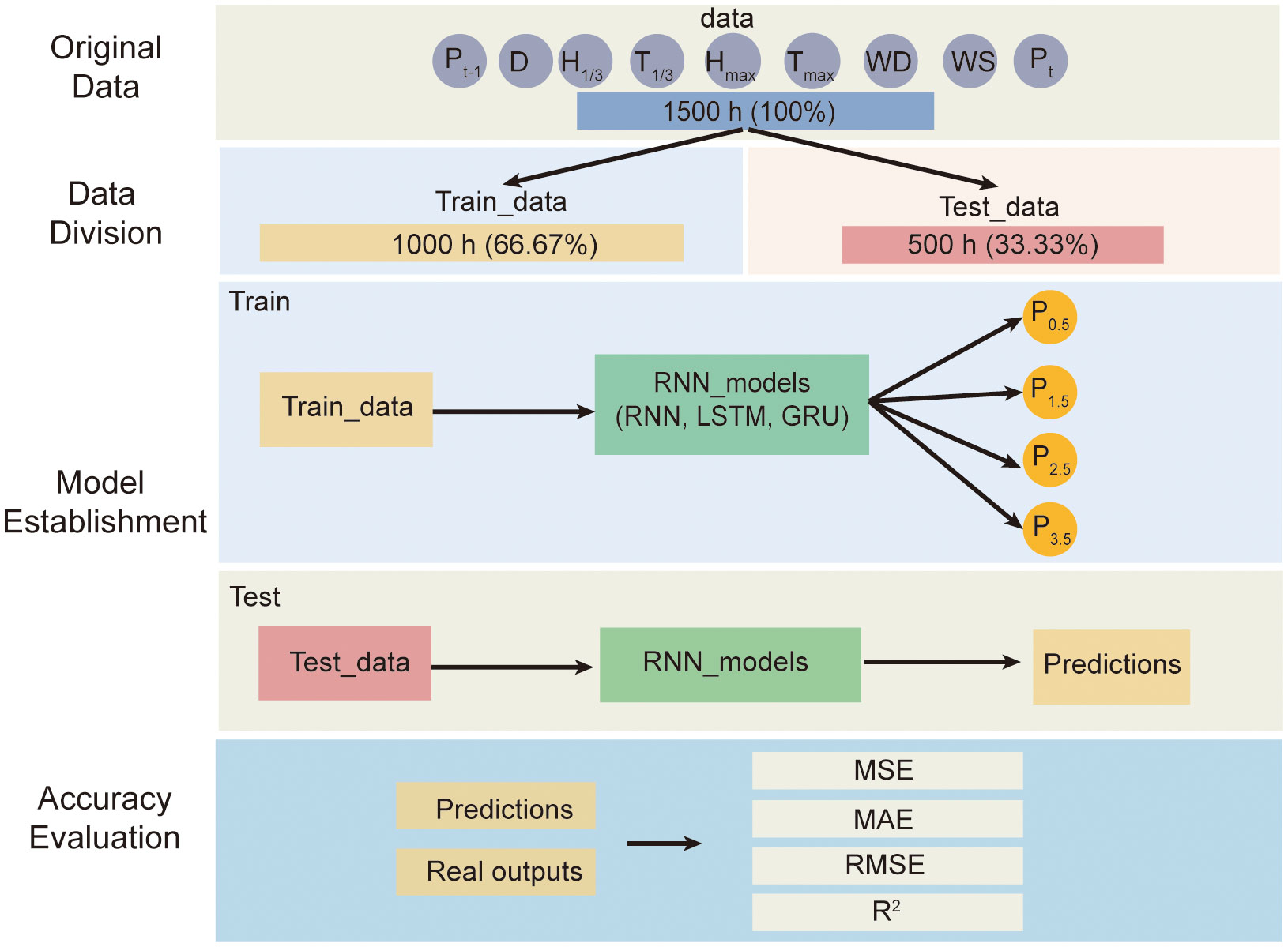
Figure 3 Flowchart of RNN model establishment.

2.4.1 Data normalization and dataset splitting

Data normalization plays a crucial role in machine learning. Diverse input data often possesses distinct dimensions and units, necessitating normalization to expedite model convergence and reduce errors during training. In this research, we employed the Min-Max normalization technique, ensuring all data is normalized within a range of zero to one.

$\begin{array}{ll}{x}_{norm}=\frac{x-x_{min}}{x_{max}-x}& (12)\end{array}$

where, x represents the original data, while $x_{norm}$ denotes the normalized data. $x_{min}$ and $x_{max}$ correspond to the minimum and maximum values within the entire dataset, encompassing both training and testing data. The Min-Max normalization technique is prevalent and effective in numerous studies. The wave-induced pore pressure dataset was split to 1000 h for training and 500 h for testing.

2.4.2 Proposed architecture

The novel architecture consists of an input layer, multiple hidden layers, and an output layer. The input layer has eight neurons corresponding to the eight calculated parameters: water depth, effective wave height, effective wave height period, maximum wave height, maximum wave height period, wind speed, wind direction, and pore pressure at time t-1. The hidden layers incorporate the beneficial features of standard RNN, LSTM and GRU models, including gating mechanisms to address the vanishing gradient problem. The output layer has four neurons corresponding to the pore pressure sensor values at four different locations.

To improve training efficiency and prevent overfitting, techniques such as dropout, and batch normalization has also been employed. Dropout can be applied to the hidden layers to introduce regularization. Batch normalization can be used to stabilize the training process by normalizing layer inputs.

2.4.3 Training and optimization

The model is trained using the Mean Squared Error (MSE) loss as the criterion, which is appropriate for regression tasks. The optimizer chosen for training is the Adam optimizer, which has been shown to work well in deep learning applications.

Model hyperparameters play a crucial role in AI modeling, and it is important to build models with different hyperparameters within a reasonable range to statistically obtain the best hyperparameters. Selecting hyperparameters that meet the accuracy requirements of the research problem is essential, as there is no universally optimal set of hyperparameters. In this study, we aimed to investigate the impact of hyperparameters on wave-induced pore pressure prediction by constructing multiple models with different parameter combinations using the standard RNN, LSTM, and GRU model (Table 1).

TABLE 1

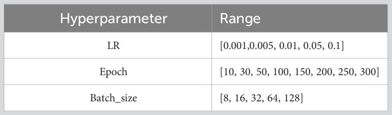
Table 1 Experimental settings of model hyperparameters.

The learning rate (LR) determines the step size during optimization, with our range [0.001, 0.1] ensuring a balance between fast convergence and model stability. Epochs, representing the number of complete passes through the dataset, range from 10 to 300, providing a comprehensive understanding of training duration versus performance trade-offs. Lastly, the batch size, varying from 8 to 128, governs the amount of data processed at once, affecting both the model’s generalization and training speed. Our chosen ranges for these hyperparameters are deliberate, striving for a broad yet meaningful exploration to pinpoint the best settings for our specific application.

2.4.4 Evaluation methods

To evaluate the accuracy of the RNN model’s predictions, we employed four evaluation metrics: Mean Squared Error (MSE), Mean Absolute Error (MAE), Root Mean Squared Error (RMSE), and R-squared (R²). These metrics provide a comprehensive understanding of the model’s performance in terms of prediction accuracy and error magnitude. The following is a description of each evaluation metric along with their respective formulas:

Mean Squared Error (MSE): MSE measures the average squared difference between the predicted and true values. It is widely used in regression tasks to quantify the prediction error. A lower MSE value indicates a better model performance. The formula for MSE is as follows:

$\begin{array}{ll}MSE=\frac{1}{n}\sum {(y_{pred}-y_{true})}^2& (13)\end{array}$

where y_pred is the predicted value, y_true is the true value, and n is the total number of data points.

Mean Absolute Error (MAE): MAE calculates the average absolute difference between the predicted and true values. It provides an easily interpretable measure of the prediction error magnitude. A lower MAE value signifies a better model performance. The formula for MAE is:

$\begin{array}{ll}MAE=\frac{1}{n}\sum \left|y_{pred}-y_{true}\right|& (14)\end{array}$

where y_pred is the predicted value, y_true is the true value, and n is the total number of data points.

Root Mean Squared Error (RMSE): RMSE is the square root of the Mean Squared Error, which provides an estimate of the prediction error in the same unit as the true values. A lower RMSE value indicates better model performance. The formula for RMSE is:

$\begin{array}{ll}RMSE=\sqrt{MSE}& (15)\end{array}$

R-squared (R²): R², also known as the coefficient of determination, measures the proportion of the variance in the true values that can be explained by the model’s predictions. It is a useful metric for evaluating the model’s goodness-of-fit. An R² value closer to 1 indicates a better model performance. The formula for R² is:

$$R^2=1-\frac{{\sum }^{}{(y_{pred}-y_{true})}^2}{{\sum }^{}{(y_{mean}-y_{true})}^2}$$

where y_pred is the predicted value, y_true is the true value, y_mean is the mean of the true values, and the summations are over all data points.

By evaluating the RNN model using these four metrics, we can gain a comprehensive understanding of the model’s prediction accuracy and error magnitude, which is essential for assessing the suitability of the model for predicting pore water pressure response within seafloor sediments under wave action.

2.4.5 Experimental settings

In this study, our methodology is structured around a multi-experiment experimental design aimed at understanding and predicting alterations in pore water pressure at varying seabed depths. The selection of input parameters should not be solely based on mathematical or statistical relevance; it must also take into account geological significance and the practicality of data acquisition. This multi-faceted approach aids in constructing a pore pressure prediction model that is both accurate and applicable. Specific experimental settings can be seen in Table 2. We outline the details of our experiment below:

TABLE 2

Table 2 Experimental design overview.

Experiment 1: Comparative analysis of RNN models

We utilize three types of RNN architectures standard RNN, LSTM, and GRU. The models are trained using a comprehensive set of eight input parameters: pore pressure at time t-1 (P_t-1, i.e., the pore pressure values of four different burial depth locations at the moment t-1), water depth (D), effective wave height (H_1/3), effective wave period (T_1/3), maximum wave height (H_max), maximum wave period (T_max), wind direction (WD), wind speed (WS). Since the goal of the first step was to compare the accuracy of different RNN networks, the full input parameters were used for the study to ensure that the information was maximized and complete. For this experiment, the models predict pore pressure at four different seabed depths: 0.5m, 1.5m, 2.5m, and 3.5m (P_0.5, P_1.5, P_2.5, P_3.5). Although the model generates pore pressure predictions at four distinct depths, the initial step emphasizes comparing model accuracies using data from a singular depth, specifically opting for the 1.5m burial depth for this comparative analysis. The model demonstrating the highest prediction accuracy for pore water pressure at this depth is designated as the ‘Best Model’.

Experiment 2: Depth-wise analysis using the best model

Upon identifying the ‘Best Model’, we extend our investigation to assess its predictive capabilities at multiple seabed depths. The model would be trained and evaluated using the same set of eight input parameters as in experiment 1. The analysis focuses on prediction accuracy at four different seabed depths, aiming to evaluate the model’s generalizability across different geotechnical conditions.

Experiments 3-5: Reduced input analysis

Considering the importance of feature relevance and the complexities of parameter acquisition, experiments 3, 4, and 5 are designed to assess the prediction accuracy when using fewer input parameters. In these experiments, we fix the first two parameters as pore pressure at time t-1 (P_t-1), water depth (D) and vary the third parameter. Specifically, experiment 3 uses effective wave height (H_1/3), experiment 4 uses, maximum wave height (H_max), and experiment 5 employs WS (wind speed) as the third input variable. H_1/3 and H_max represent two statistical cases of waves, and the use of WS instead of wave height is to be explored to see if the use of wind speeds, which are taught to be easily accessible, can be used as a substitute for wave parameters. These experiments utilize the ‘Best Model’ identified in experiment 1 for predictions.

2.4.6 Implementation

The novel architectures were implemented using PyTorch, a popular deep learning framework, which offer extensive libraries and tools for neural network development. The calculating device is a workstation named MacBook Pro 16 with CPU of M1 Pro, 16G of RAM.

3 Results and discussions

3.1 Accuracy comparison of standard RNN, LSTM and GRU

To compare the prediction accuracy of the standard RNN, LSTM and GRU models on the wave-induced pore pressure response problem, the same train and test datasets were used for all the three models. Figure 4 shows the real pore pressure variation values compared with the predicted values and the absolute error statistics among the three different RNN models using box chart and CDF (Cumulative Distribution Function), respectively. As observed in Figure 4A, the pore pressure prediction results using the three RNN models show results and trends similar to the actual pore pressure values. Since the results predicted by the three RNN models were relatively close, we used mathematical statistical analysis for further comparison. Figure 4B shows the box plots of the absolute errors of the prediction results for the three RNN models of all the 1000 test data (two data per hour), with the box statistics ranging from 5% to 95% of the absolute errors. As can be observed from Figure 4, both the maximum error value, 95% error value, median, and mean, the absolute error of GRU is smaller than that of LSTM is smaller than that of standard RNN. Figure 4C uses the CDF to evaluate the statistics of the error values predicted by different models, and the models with a larger proportion of smaller absolute error values perform better. It is clear from the Figure 4C that the overall GRU curve lies above the LSTM and standard RNN. Combining the two statistical results, the model accuracy in the problem of predicting the pore pressure response of the pozzolanic sediment is shown as GRU>LSTM> standard RNN.

FIGURE 4

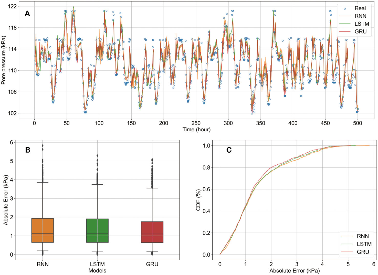
Figure 4 Comparison of prediction accuracies of standard RNN, LSTM and GRU. (A) is the comparison among real PWP and predict PWP; (B) is the prediction absolute error of the three RNN models; (C) is the CDF of the prediction errors of the three RNN models.

Table 3 presents the performance of different RNN models in terms of prediction accuracy. The metrics evaluated in this study include Mean Squared Error (MSE), Mean Absolute Error (MAE), Root Mean Squared Error (RMSE), and R-squared (R²) coefficient. The standard RNN model achieved an MSE of 3.33, an MAE of 1.45, an RMSE of 1.83, and an R² value of 0.80. The LSTM model performed slightly better with an MSE of 3.13, an MAE of 1.41, an RMSE of 1.77, and an R² value of 0.81. The GRU model showed the best performance among the three models, with an MSE of 2.92, an MAE of 1.36, an RMSE of 1.71, and an R² value of 0.83. Based on these results, it can be concluded that the GRU model outperformed the RNN and LSTM models in terms of prediction accuracy. The GRU model achieved lower error values (MSE, MAE, and RMSE) and a higher R² value, indicating a better fit to the data and improved ability to explain the variance in the predictions.

TABLE 3

Table 3 Performance of prediction accuracy using different RNN models.

The GRU’s superior performance can be attributed to its architectural simplicity, as it strikes a balance between RNNs and LSTMs by capturing long-term dependencies with fewer gates. This results in faster training and fewer parameters. Additionally, GRUs effectively address the vanishing gradient problem and their gating mechanism can be more adaptive for specific problems like the wave-induced pore pressure response. In situations where only recent past events are crucial, the GRU’s design becomes advantageous. Compared to LSTMs, GRUs can be more efficient for datasets that aren’t extensive or when long-term dependencies are straightforward. The GRU’s simpler design may also reduce overfitting risks. In essence, the GRU’s design and efficiency combined with the unique dynamics of our dataset led to its optimal performance.

3.2 Prediction accuracies in different depth

In order to investigate the prediction of pore pressure values at different depths of seabed burial, we have used the model established by GRU to predict the pore pressure at 0.5, 1.5, 2.5, and 3.5m locations. Figure 5 shows the comparison between the predicted and true values of pore pressure at different seabed depths of burial. As can be observed from the Figure 5, the predicted results of the GRU model are closer to the actual pore pressure values, which can simulate and predict the pore pressure at different burial depth locations accurately.

FIGURE 5

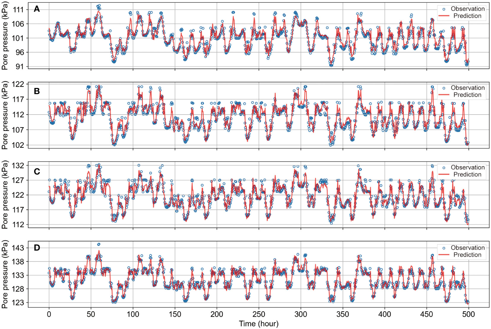
Figure 5 GRU-based pore pressure prediction results at different depths. (A–D) are the comparison between the observed and real values of pore pressure at 0.5m, 1.5m, 2.5m, and 3.5m burial depths, respectively. .

Figure 6 demonstrates the absolute error statistics using box statistics and CDF charts for 30 replicate tests at different depth locations. From Figure 6A, it can be observed that the overall absolute error is less than 4 kPa at all depth locations, and the median absolute error is less than 1 kPa. The absolute error value increases gradually from 0.5 m to 2.5 m, but is minimal at 3.5 m. Figure 6B shows more clearly the comparison of the absolute error between different depths, with the highest CDF curve at the 3.5m depth position, followed by the crossover at the 0.5m and 1.5m positions, and the lowest curve at the 2.5m position. Meanwhile, the CDF curves at all depth positions exceeded 80% at an absolute error of 2 kPa. It shows that the model can accurately predict the pore pressure variation at different depths. The analysis of the two subplots in Figure 6 shows that the GRU-based model can accurately predict the pore pressure variation at different depths (the median of repeated tests is less than 1 kPa), and there is no necessary connection between the depth and the accuracy.

FIGURE 6

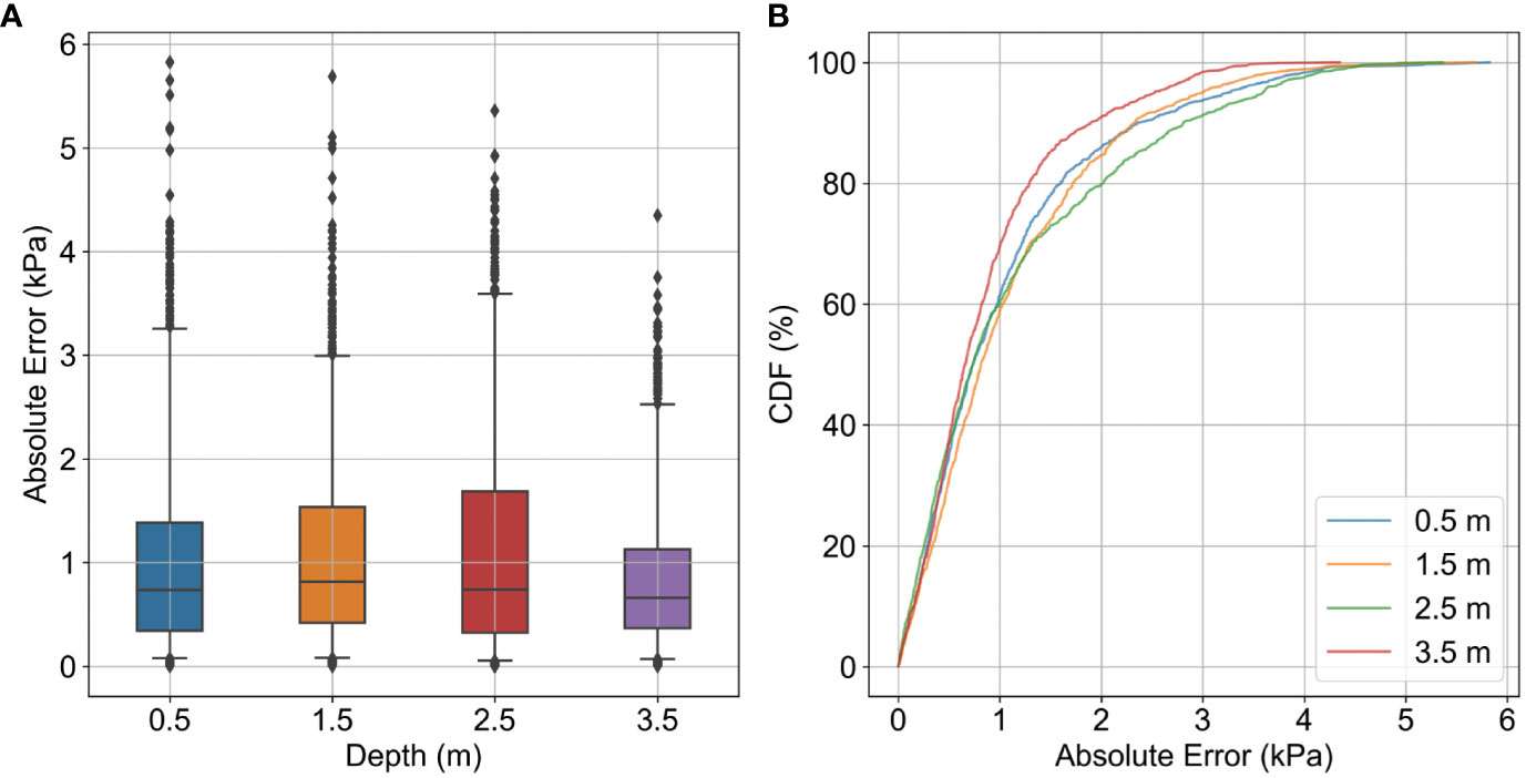
Figure 6 Statistical results of pore pressure prediction for different seabed burial depth locations. (A) is the prediction absolute error of pore pressure at four different seabed burial depth locations; (B) is the CDF of the prediction errors of pore pressure at four different seabed burial depth locations.

Table 4 presents the performance metrics of different depth configurations using the GRU model on the test dataset. It can be observed that increasing the depth of the GRU model from 0.5 to 1.5 led to a slight improvement in performance, but the performance decreased when the depth was further increased to 2.5. Depth 3.5 demonstrates the best performance, with MSE 1.58, MAE 1.13, RMSE 0.85, and R² 0.92. These results indicate that increasing the depth can have mixed effects on the model’s accuracy.

TABLE 4

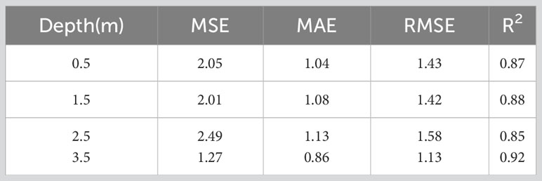
Table 4 Performance of prediction accuracy at different depth using GRU model.

In Section 3.2, we noted subtle variances in the Mean Absolute Errors (MAEs) across different seabed depths. It’s essential to underscore that these variations, although discernible in our graphical representations, translate to only minor discrepancies in absolute terms. A change of a few tenths of a kPa in pore pressure is not typically impactful in practical geotechnical applications. These slight disparities in MAEs might be due to inherent natural variations or potential inconsistencies during data acquisition rather than reflecting any significant geological distinctions. The consistent performance of the GRU model across these depths, even with these minor fluctuations, underscores its resilience and versatility in handling different geological scenarios. Overall, it is shown that the accuracy of the GRU model prediction results is independent of the sediment burial location and that the model can accurately predict pore pressure at all burial locations.

3.3 Comparison of GRU models with different input parameters

In this study, four different Gated Recurrent Unit (GRU) models were trained using various combinations of input parameters to predict pore pressure at varying seabed burial depths. The input parameter settings can be seen from Table 2 (2) ~ (5), which contain control group [Table 2 (2)], significant wave height group [Table 2 (3)], maximum wave height [Table 2 (4)], and wind speed group [Table 2 (5)].

As seen in Figure 7A, the model that used significant wave height (H_1/3) as the wave parameter exhibited the lowest average MAE value at 1.016, followed by wind speed (1.035) and maximum wave height (1.038). Interestingly, the control group model that employed all parameters showed a slightly worse performance, with an average MAE of 1.063. From Figure 7B we can see that, A similar trend was observed for MSE values. The model trained using significant wave height (H_1/3) demonstrated the lowest MSE of 1.894, followed by the control group, maximum wave height, and wind speed, which had values of 2.012, 1.999, and 1.947 respectively.

FIGURE 7

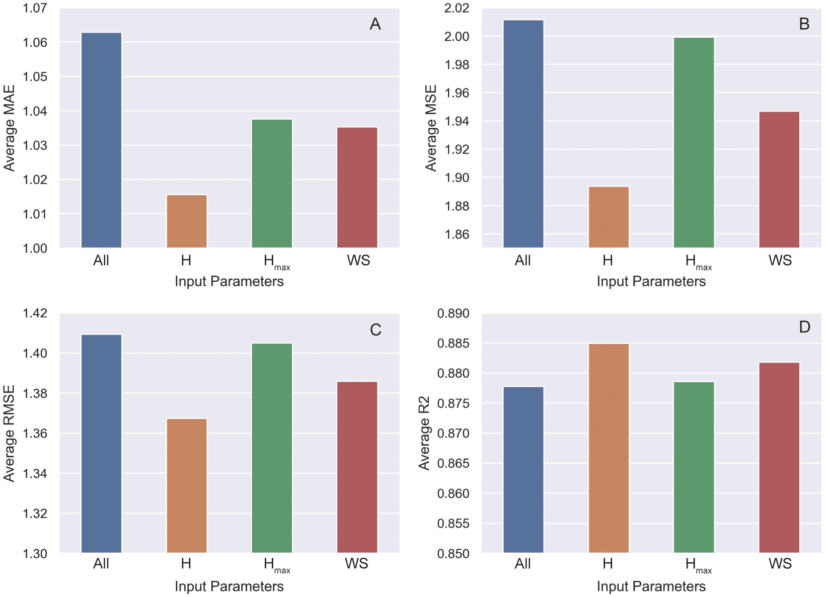
Figure 7 Statistical averages of model accuracy with different input parameters. Where All is the experiments using all input parameters; H is the experiment using pore pressure at time t-1, water depth and significant wave height; H_max is the experiment using pore pressure at time t-1, water depth and maximum wave height; WS is the experiment using pore pressure at time t-1, water depth and wind speed. H is the (A) is the average MAE; (B) is the average MSE; (C) is the average RMSE; (D) is the average R².

It can be seen from Figure 7C that, the model with significant wave height (H_1/3) also outperformed in terms of RMSE, with an average value of 1.367, better than the control group (1.409), maximum wave height (1.405), and wind speed (1.386). As for the R² values (Figure 7D) indicate that the prediction accuracy of all models was relatively high, ranging from 0.878 to 0.885. The model using significant wave height (H_1/3) as an input parameter showed the highest R² value of 0.885.

Overall, the models that used different input parameters demonstrated respectable accuracy with MAE errors all below 1.1 kPa. Among the different input parameters, significant wave height performed the best, followed by wind speed, maximum wave height, and the control group with all parameters. Upon analyzing the underlying reasons, it becomes evident that the significant wave height (H_1/3) offers a more holistic representation of wave conditions. This parameter accounts for both the average and more extreme wave heights, thereby providing a balanced input for the model. On the other hand, maximum wave height (H_max) represents more extreme cases, and hence is not a good proxy for the overall wave conditions, leading to slightly greater computational errors. The use of wind speed (WS) as an alternative parameter is also noteworthy. While not as effective as wave height in representing wave conditions, it provides a reasonable approximation when wave data are not readily available.

Therefore, it can be concluded that for best results, significant wave height (H_1/3) should be used for calculations when conditions allow. When wave parameters are hard to acquire, using wind speed to represent wave magnitude is also acceptable.

4 Future work

We employed three RNN models to effectively model long time series pore pressure data obtained from marine field monitoring, enabling accurate predictions up to a duration of 500 hours. This demonstrates the valuable utility of deep learning methods for addressing the wave-induced pore pressure problem and offers insights for tackling time series prediction challenges in the field of marine geology.

However, the accuracy of the model is notably influenced by the training data, which is inherent to the working principle of deep learning models. Achieving an accurate model relies on having complete and realistic input data encompassing various influential factors. Incomplete or inaccurate input data will inevitably lead to inaccuracies in the resulting model. Therefore, the acquisition and organization of data become crucial focal points in deep learning-based modeling. Furthermore, the deep learning model developed in this study is tailored specifically to the powdered soil seabed conditions in the Yellow River estuary and may not be suitable for all study areas. This is a characteristic of deep learning models—they excel at nonlinear modeling within a given data range but lack generalization beyond that range. When modeling pore pressure prediction in other areas, it remains necessary to gather a substantial amount of data and information on geological parameters.

When establishing a deep learning geological model, it is important to consider not only the mathematical significance of optimal prediction accuracy but also the richness and completeness of the model parameters in a geological sense. For instance, in this study, when discussing the influencing factors of wave-induced pore pressure prediction, although the correlation coefficients of parameters such as wave height and wind speed with the pore pressure at time t-1 are only one-fourth of that with water depth, they still need to be considered during modeling. Only wave periods with very low correlation can be discarded. This is because deep learning models are prone to overfitting when trained excessively. Even though the two strongly correlated parameters in this problem can accurately predict pore pressure, it does not imply that only these two parameters can be used for accurate predictions in other regions. Geologically significant parameters, such as wave characteristics and wind speed, need to be included in the model’s input parameters.

In future research, we will leverage the findings of this study to further explore novel techniques and methods for predicting wavelike pore pressure. While this study utilized field monitoring data as input parameters, it is important to address the high data acquisition cost. Investigating whether the relationship of wave-induced pore pressure can be established directly using easily accessible parameters such as water depth, sediment characteristics, wave properties, current conditions, and sea wind patterns will be a key focus of our future work. Additionally, while the current study emphasizes long-term pore pressure prediction in half-hour intervals, we acknowledge the importance of understanding and predicting rapid changes that occur in much shorter timescales. As soil liquefaction in response to strong and continuous wave action can transpire within minutes or even seconds, future endeavors will prioritize finer temporal resolutions. This will allow us to capture and predict imminent sediment behaviors, offering a more holistic and practical insight into seabed dynamics under varying wave conditions. By merging the findings from both long-term and short-term predictions, we aim to offer a comprehensive tool for marine geologists and engineers in their efforts to anticipate and mitigate liquefaction risks.

5 Conclusions

In this study, we employed three deep learning models, namely, the standard RNN, LSTM, and GRU, to model and predict the variation of pore pressure under long time series of wave actions obtained from in-situ marine monitoring. We compared the accuracy of these three models and ultimately identified the most suitable model for wave-induced pore pressure prediction. We conducted predictions with different depths, discussed the effects of model hyperparameters, input parameters on model prediction accuracy. The main conclusions are as follows:

(1) Deep learning models can accurately predict the response of pore pressure to ocean waves. All three models achieved a prediction horizon of 500 hours and kept the absolute error within 2 kPa. Among them, the GRU model exhibited the highest accuracy.

(2) When predicting wave-induced pore pressure at different seabed depths, the GRU model achieved a relatively high accuracy (MAE around 1 kPa). There was no significant correlation between prediction accuracy and depth.

(3) The model built using the pore pressure at the previous moment, water depth, and effective wave height as input parameters predicted the most accurate values. When aiming for easily obtainable input parameters, wind speed can be effectively used in place of the effective wave height, without compromising prediction accuracy significantly.

(4) The ability to predict pore pressure under long time series of wave actions is crucial, especially considering the continual and varying influence of waves over extended periods. Such long-duration predictions provide a more realistic representation of seafloor pore pressure and liquefaction response under persistent wave action. This research underscores the significance of long time series predictions in understanding the potential risks associated with seafloor sediment stability in marine environments.

Data availability statement

The raw data supporting the conclusions of this article will be made available by the authors, without undue reservation.

Author contributions

XD: Conceptualization, Data curation, Funding acquisition, Project administration, Resources, Software, Visualization, Writing – original draft, Writing – review & editing. YFS: Validation, Writing – review & editing. YPS: Methodology, Writing – review & editing. YY: Methodology, Writing – review & editing. QZ: Resources, Writing – review & editing.

Funding

The author(s) declare financial support was received for the research, authorship, and/or publication of this article. This research was funded by the Foundation item: The National Natural Science Foundation of China under contract NO. 42102326; the Basic Scientific Fund for National Public Research Institutes of China under contract NO. 2022Q05; and The Shandong Provincial Natural Science Foundation, China under contract NO. ZR2020QD073.

Acknowledgments

The authors would like to thank to the developers who proposed the Pytorch deep learning package (https://pytorch.org/), which support the RNN modeling in this paper.

Conflict of interest

The authors declare that the research was conducted in the absence of any commercial or financial relationships that could be construed as a potential conflict of interest.

Publisher’s note

All claims expressed in this article are solely those of the authors and do not necessarily represent those of their affiliated organizations, or those of the publisher, the editors and the reviewers. Any product that may be evaluated in this article, or claim that may be made by its manufacturer, is not guaranteed or endorsed by the publisher.

References

Balogun A.-L., Tella A., Baloo L., Adebisi N. (2021). A review of the inter-correlation of climate change, air pollution and urban sustainability using novel machine learning algorithms and spatial information science. Urban Climate 40, 100989. doi: 10.1016/j.uclim.2021.100989

CrossRef Full Text | Google Scholar

Chang K.-T., Jeng D.-S. (2014). Numerical study for wave-induced seabed response around offshore wind turbine foundation in Donghai offshore wind farm, Shanghai, China. Ocean Eng. 85, 32–43. doi: 10.1016/j.oceaneng.2014.04.020

CrossRef Full Text | Google Scholar

Cho K., van Merrienboer B., Gulcehre C., Bahdanau D., Bougares F., Schwenk H., et al. (2014). Learning phrase representations using RNN encoder-decoder for statistical machine translation. doi: 10.48550/arXiv.1406.1078

CrossRef Full Text | Google Scholar

Collico S., Arroyo M., Urgeles R., Gràcia E., Devincenzi M., Peréz N. (2020). Probabilistic mapping of earthquake-induced submarine landslide susceptibility in the South-West Iberian margin. Mar. Geology 429, 106296. doi: 10.1016/j.margeo.2020.106296

CrossRef Full Text | Google Scholar

Du X., Sun Y., Song Y., Sun H., Yang L. (2023). A comparative study of different CNN models and transfer learning effect for underwater object classification in side-scan sonar images. Remote Sens. 15, 593. doi: 10.3390/rs15030593

CrossRef Full Text | Google Scholar

Du X., Sun Y., Song Y., Xiu Z., Su Z. (2022). Submarine landslide susceptibility and spatial distribution using different unsupervised machine learning models. Appl. Sci. 12, 10544. doi: 10.3390/app122010544

CrossRef Full Text | Google Scholar

Du X., Sun Y., Song Y., Zhu C. (2021). In-situ observation of wave-induced pore water pressure in seabed silt in the yellow river estuary of China. J. Mar. Environ. Eng. 10, 305–317.

Google Scholar

Duan L., Qin C., Zhou J., Tang G., Wang D., Fan M. (2023). Numerical study of regular wave-induced oscillatory soil response during the caisson installation. Ocean Eng. 281, 114876. doi: 10.1016/j.oceaneng.2023.114876

CrossRef Full Text | Google Scholar

Gao S., Huang J., Li Y., Liu G., Bi F., Bai Z. (2021). A forecasting model for wave heights based on a long short-term memory neural network. Acta Oceanol. Sin. 40, 62–69. doi: 10.1007/s13131-020-1680-3

CrossRef Full Text | Google Scholar

Gers F. A., Schmidhuber J., Cummins F. (2000). Learning to forget: continual prediction with LSTM. Neural Comput. 12, 2451–2471. doi: 10.1162/089976600300015015

PubMed Abstract | CrossRef Full Text | Google Scholar

He K., Ye J. (2023a). Dynamics of offshore wind turbine-seabed foundation under hydrodynamic and aerodynamic loads: A coupled numerical way. Renewable Energy 202, 453–469. doi: 10.1016/j.renene.2022.11.029

CrossRef Full Text | Google Scholar

He K., Ye J. (2023b). Seismic dynamics of offshore wind turbine-seabed foundation: Insights from a numerical study. Renewable Energy 205, 200–221. doi: 10.1016/j.renene.2023.01.076

CrossRef Full Text | Google Scholar

Hochreiter S., Schmidhuber J. (1997). Long short-term memory. Neural Comput. 9, 1735–1780. doi: 10.1162/neco.1997.9.8.1735

PubMed Abstract | CrossRef Full Text | Google Scholar

Hu C., Li X., Ji C., Jiao X., Jia Y. (2023). In-situ observation of seabed vertical deformation in Yellow River Delta under storm surges. Mar. Petroleum Geology 152, 106250. doi: 10.1016/j.marpetgeo.2023.106250

CrossRef Full Text | Google Scholar

Ji S., Dawen Y., Shen C., Li W., Xu Q. (2020). Landslide detection from an open satellite imagery and digital elevation model dataset using attention boosted convolutional neural networks. Landslides 17:1337–1352. doi: 10.1007/s10346-020-01353-2

CrossRef Full Text | Google Scholar

Jia Y., Zhang L., Zheng J., Liu X., Jeng D.-S., Shan H. (2014). Effects of wave-induced seabed liquefaction on sediment re-suspension in the Yellow River Delta. Ocean Eng. 89, 146–156. doi: 10.1016/j.oceaneng.2014.08.004

CrossRef Full Text | Google Scholar

Jones S., Kasthurba A. K., Bhagyanathan A., Binoy B. V. (2021). Landslide susceptibility investigation for Idukki district of Kerala using regression analysis and machine learning. Arab J. Geosci 14, 838. doi: 10.1007/s12517-021-07156-6

CrossRef Full Text | Google Scholar

Laurenti L., Tinti E., Galasso F., Franco L., Marone C. (2022). Deep learning for laboratory earthquake prediction and autoregressive forecasting of fault zone stress. Earth Planetary Sci. Lett. 598, 117825. doi: 10.1016/j.epsl.2022.117825

CrossRef Full Text | Google Scholar

Lawson E., Smith D., Sofge D., Elmore P., Petry F. (2017). Decision forests for machine learning classification of large, noisy seafloor feature sets. Comput. Geosciences 99, 116–124. doi: 10.1016/j.cageo.2016.10.013

CrossRef Full Text | Google Scholar

Liu X., Chai N., Zhao H., Jeng D.-S., Zhou J. (2023). Numerical investigation into wave-induced progressive liquefaction based on a two-layer viscous fluid system. Comput. Geotechnics 159, 105447. doi: 10.1016/j.compgeo.2023.105447

CrossRef Full Text | Google Scholar

Maxwell K., Rajabi M., Esterle J. (2019). Automated classification of metamorphosed coal from geophysical log data using supervised machine learning techniques. Int. J. Coal Geology 214, 103284. doi: 10.1016/j.coal.2019.103284

CrossRef Full Text | Google Scholar

Orland E., Roering J. J., Thomas M. A., Mirus B. B. (2020). Deep learning as a tool to forecast hydrologic response for landslide-prone hillslopes. Geophysical Res. Lett. 47, e2020GL088731. doi: 10.1029/2020GL088731

CrossRef Full Text | Google Scholar

Politikos D. V., Fakiris E., Davvetas A., Klampanos I. A., Papatheodorou G. (2021). Automatic detection of seafloor marine litter using towed camera images and deep learning. Mar. pollut. Bull. 164, 111974. doi: 10.1016/j.marpolbul.2021.111974

PubMed Abstract | CrossRef Full Text | Google Scholar

Rumelhart D. E., Hinton G. E., Williams R. J. (1986). Learning representations by back-propagating errors. Nature 323, 533–536. doi: 10.1038/323533a0

CrossRef Full Text | Google Scholar

Song Y., Sun Y., Wang Z., Du X., Song B., Dong L. (2022). In situ observation of silt seabed pore pressure response to waves in the subaqueous yellow river delta. J. Ocean Univ. China 21, 1154–1160. doi: 10.1007/s11802-022-4843-3

CrossRef Full Text | Google Scholar

Wang H., Liu H. (2016). Evaluation of storm wave-induced silty seabed instability and geo-hazards: A case study in the Yellow River delta. Appl. Ocean Res. 58, 135–145. doi: 10.1016/j.apor.2016.03.013

CrossRef Full Text | Google Scholar

Wang Z., Sun Y., Jia Y., Shan Z., Shan H., Zhang S., et al. (2020). Wave-induced seafloor instabilities in the subaqueous Yellow River Delta—initiation and process of sediment failure. Landslides 17, 1849–1862. doi: 10.1007/s10346-020-01399-2

CrossRef Full Text | Google Scholar

Wei X., Zhang L., Yang H.-Q., Zhang L., Yao Y.-P. (2021). Machine learning for pore-water pressure time-series prediction: Application of recurrent neural networks. Geosci. Front. 12, 453–467. doi: 10.1016/j.gsf.2020.04.011

CrossRef Full Text | Google Scholar

Xu G., Liu Z., Sun Y., Wang X., Lin L., Ren Y. (2016). Experimental characterization of storm liquefaction deposits sequences. Mar. Geology 382, 191–199. doi: 10.1016/j.margeo.2016.10.015

CrossRef Full Text | Google Scholar

Yang B., Yin K., Lacasse S., Liu Z. (2019). Time series analysis and long short-term memory neural network to predict landslide displacement. Landslides 16, 677–694. doi: 10.1007/s10346-018-01127-x

CrossRef Full Text | Google Scholar

Ye J., He K. (2021). Dynamics of a pipeline buried in loosely deposited seabed to nonlinear wave & current. Ocean Eng. 232, 109127. doi: 10.1016/j.oceaneng.2021.109127

CrossRef Full Text | Google Scholar

Ye J., Jeng D.-S., Chan A. H. C., Wang R., Zhu Q. C. (2017). 3D integrated numerical model for Fluid-Structures-Seabed Interaction (FSSI): Loosely deposited seabed foundation. Soil Dynamics Earthquake Eng. 92, 239–252. doi: 10.1016/j.soildyn.2016.10.026

CrossRef Full Text | Google Scholar

Ye J., Jeng D.-S., Wang R., Zhu C. (2015). Numerical simulation of the wave-induced dynamic response of poro-elastoplastic seabed foundations and a composite breakwater. Appl. Math. Model. 39 (1), 322–347. doi: 10.1016/j.apm.2014.05.031

CrossRef Full Text | Google Scholar

Zennaro F., Furlan E., Simeoni C., Torresan S., Aslan S., Critto A., et al. (2021). Exploring machine learning potential for climate change risk assessment. Earth-Science Rev. 220, 103752. doi: 10.1016/j.earscirev.2021.103752

CrossRef Full Text | Google Scholar

Zhang H., Lu Y., Liu X., Li X., Wang Z., Ji C., et al. (2023). Morphology and origin of liquefaction-related sediment failures on the Yellow River subaqueous delta. Mar. Petroleum Geology 153, 106262. doi: 10.1016/j.marpetgeo.2023.106262

CrossRef Full Text | Google Scholar