The use of spaceborne lidar to map Antarctic krill distributions and biomass in the Southern Ocean

1 Introduction

Antarctic krill (Euphausia superba), is a small crustacean (Santa Cruz et al., 2018) that is one of the largest known single living resources on Earth (Siegel et al., 1998; Nicol and Foster, 2003; Dai et al., 2012). Antarctic krill are widely distributed in the waters of the circum-Antarctic continental shelf, especially in the waters surrounding the Antarctic Peninsula. It feeds on phytoplankton and is a major food source for higher trophic level organisms (Santa Cruz et al., 2018), and is therefore a keystone species in the Southern Ocean ecosystems (Nicol et al., 2008; Stowasser et al., 2012; Zhu, 2012). Due to the high nutritional value (Yoshitomi et al., 2007; Ericson et al., 2018), abundant resources and key ecological status, Antarctic krill has a huge commercial development value (Guoqin et al., 2022), and its resource distribution and environmental impact factors are the important content of the research of scholars from various countries (Siegel, 2005; Li et al., 2022).

The krill resource has been assessed several times. In 1981, FIBEX (First International BIOMASS Experiment) conducted the first large-scale biomass survey of krill resources by acoustic assessment, and the results showed that the biomass of krill in the sea area between 15°E and 30°E, south of 62°S, was 9.05×10⁵ tons (Hampton, 1985). In 1985, Law (Laws, 1985) based on the predator consumption method combined with the P/B coefficient gave a krill biomass of about 8.46×10⁸ tons. In the same year, Clark (Clarke, 1985) derived a krill biomass of 1.80 to 9.00×10⁸ tons from phytoplankton consumption based on the bait method. Siegel (Siegel, 2005) synthesized acoustic data collected from multiple surveys, evaluated the density of acoustic detections and estimated biomass in different sea areas, and derived results that the total krill biomass in Antarctic waters ranged from 6.74×10⁷ to 2.97×10⁸ tons. The Commission for the Conservation of Antarctic Marine Living Resources (CCAMLR) reassessed the biomass of Antarctic krill in the fishing area 48 in 2010 and determined that the biomass of krill in the area was 6.03×10⁷ tons (Ccamlr, 2010).

The acoustic method is the official krill stock assessment method used by CCAMLR, with the advantages of wide sampling range, high resolution, and high accuracy of the assessment results without causing harm to krill. However, there are some disadvantages of this method such as poor accuracy of acoustic data within 20m of the sea surface due to background noise (Yang and Zhu, 2018). Large-scale acoustic resource assessments are routinely carried out in the Antarctic by scientific survey vessels and are therefore more costly. Commercial krill fishery data have also been used for resource assessment, however commercial krill fishery operations are concentrated in time and operate at different spatial scales, which may affect the accuracy of krill resource assessment. As an active remote sensing technology, LiDAR has the advantages of high resolution, flexibility and efficiency (Renhe, 1994; Liu et al., 2015), and is capable of obtaining information on the vertical structure of phytoplankton and marine environmental factors, such as temperature, sea ice and chlorophyll, on a large scale and periodically (Sullivan et al., 2010; Behrenfeld et al., 2017; Chen and Pan, 2019; Yunfeng et al., 2020). Cloud aerosol lidar and infrared pathfinder satellite observations (CALIPSO) launched by NASA provides imagery that supports the characterization of the vertical structure of plankton near the ocean surface (Lu et al., 2021). The orthogonally polarized cloud aerosol lidar (CALIOP) carried on CALIPSO is the first dual-polarized lidar to provide a global vertical profile of diurnal elastic backscatter (Lu et al., 2014). Yang et al. (2022) studied the characterization and formation conditions of phytoplankton thin layers in the northern Gulf of Mexico using airborne LiDAR data obtained from NOAA. Chen et al. provided a comprehensive understanding of the vertical distribution of optical properties in different seas from the East China Sea to the South China Sea using a LiDAR system (Chen et al., 2022; Zhang and Chen, 2022).In addition, LiDAR is capable of acquiring high-resolution data at night and at high latitudes (Liu et al., 2018). Zhang et al. (2023) proposed an innovative feed-forward neural network (FFNN) model for inversion of subsurface particle backscattering coefficient (bbp), chlorophyll concentration (Chl), and total particulate organic carbon (POC) from satellite-borne lidar. The interannual variability of ecosystems in polar regions was analyzed by estimating the nonlinear relationship between lidar signals and bio-optical parameters through FFNN.

In this paper, based on the relationship between the krill CPUE and environmental factors, we combined the active and passive remote sensing data to establish a krill CPUE inversion model and prediction, with a view to providing continuous and stable krill habitat distribution and stock assessment data. In the following part, the data and methods are described in Section 2; the modeling results of several approaches are compared and the spatial distribution of the climatic state months of Antarctic krill is plotted in Section 3; the effects of various environmental factors on Antarctic krill are discussed in Section 4; and finally, conclusions and perspectives are presented in Section 5.

2 Materials and methods

2.1 Study area

The Antarctic region is divided into three main fishing areas (Figure 1A): fishing area 48, 58 and 88. According to the CCAMLR conservation measures, fishing area 58 and 88 have been closed to fishing since 1997 and 1993, respectively, so the study area for this paper is fishing area 48. There are six subareas in area 48 (Figure 1B), of which fishing is currently only conducted in subareas 481 to 484, and the fishery in subarea 486 is an exploratory fishery.

Figure 1

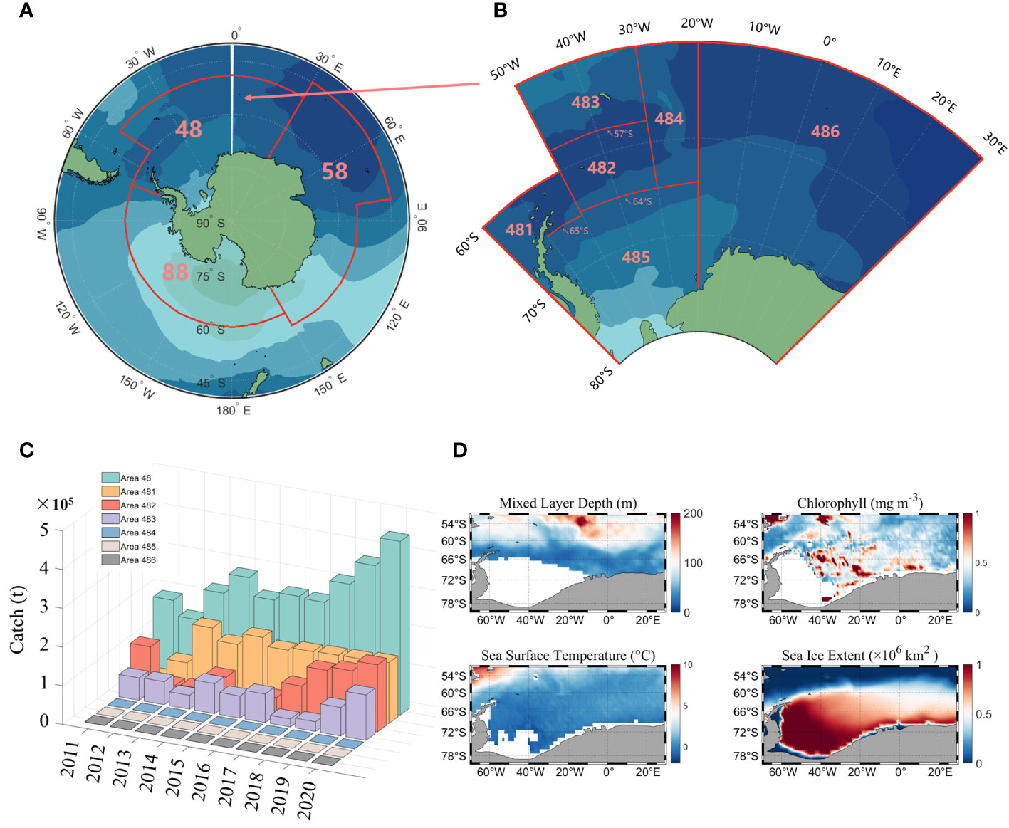
Figure 1 The designated fishing areas established by the CCAMLR (A), as well as the specific subarea within fishing area 48 (B); Statistical chart of the global production of Antarctic krill in fishing area 48 between the years 2011 and 2020 (C) and the distribution of climatic states for environmental factors in fishing area 48 (D).

2.2 In-situ and remote sensing data

Antarctic krill fishery data were obtained from CCAMLR (https://www.ccamlr.org/), which include year, month, fishing area, catch(tons) and fishing effort (day). The time span is from 2011 to 2020, with a monthly resolution and the statistics of krill production are shown in Figure 1C.

Environmental factor data (Figure 1D) include mixed layer depth (MLD), chlorophyll (CHL), sea surface temperature (SST), and sea ice extent (SIE). MLD and SST data are derived from the monthly global physical variable reprocessing product ARMOR3D L4 published by the Copernicus Marine Environmental Monitoring Service (http://resources.marine.copernicus.eu/product-detail/MULTIOBS_GLO_PHY_TSUV_3D_MYNRT_015_012). Chlorophyll data consist of both passive and active remotely sensed data, with passive remotely sensed data derived from monthly averaged MODIS-Aqua Level 3 data at a resolution of 4 km (http://oceancolor.gsfc.nasa.gov). The active remote sensing data are from the orthogonally polarized cloud aerosol lidar (CALIOP) developed by NASA and the National Center for Space Studies (CNES), which includes the CALIPSO Level-1B V4.10 product and the Level-2 Merged Layer V4.20 product (http://orca.science.oregonstate.edu/lidar_nature_2019.php). SIE data are from the Copernicus Climate Change Service (https://climate.copernicus.eu/sea-ice).

2.3 CPUE inversion method

The research method of this paper mainly includes matching the krill CPUE with MLD, CHL (MODIS), SST and SIE according to the time scale, and substituting the matched data into the GLM, ANN and SVM models for modeling, respectively. The relationship between environmental factors and CPUE was calculated and compared to validate the effects of the three models. Then, the particle backscattering coefficient (b_bp) of CALIPSO was processed, and the feed-forward neural network (FFNN) model was used to establish the relationship between b_bp and CHL of MODIS, and to invert the diurnal CHL data of Antarctic region. Finally, the inverted diurnal CHL data were matched with MLD, SST and SIE according to the CHL latitude/longitude resolution (2°×1°) and input into the optimal model for krill CPUE prediction. Nominal CPUE and predicted CPUE were sorted out by calculating the coefficient of determination (R²) and root mean square error (RMSE), and the correlation between the two was calculated, so as to analyze the influence of spatial and temporal factors and environmental factors on the krill CPUE and to evaluate its resources. The flow chat is shown in Figure 2.

Figure 2

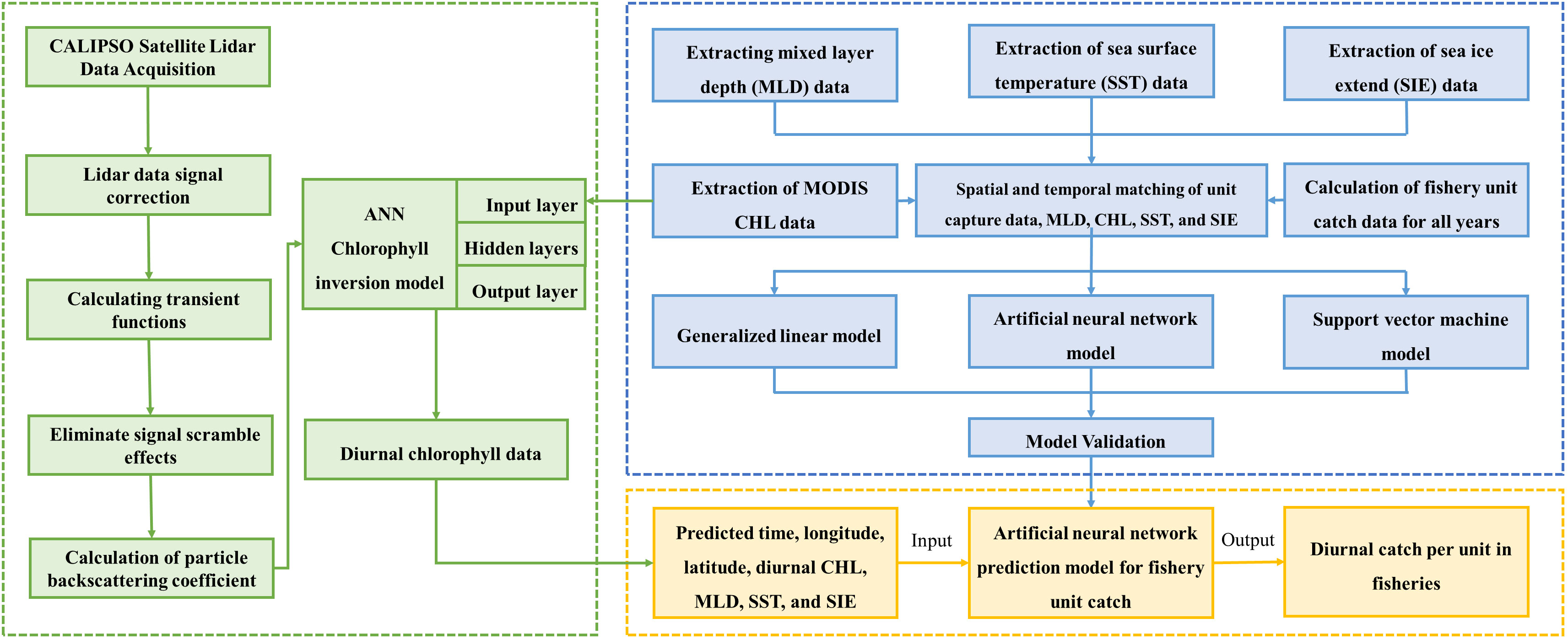
Figure 2 Flow chart of CPUE inversion method.

First, the Antarctic krill catch data need to be standardized to express the abundance of krill fishery resources in terms of nominal CPUE, and krill CPUE (t/d) is defined as the total catch (t) per day (d), year i, month j, k longitude, l latitude. The CPUE (Equation 1) is calculated as.

$\begin{array}{ll}\mathit{C}\mathit{P}\mathit{U}{\mathit{E}}_{i,j,k,l}= \frac{{\sum }^{}\mathit{C}\mathit{a}\mathit{t}\mathit{c}{\mathit{h}}_{i,j}}{{\sum }^{}{\mathit{E}}_{i,j}}& (1)\end{array}$

Where ${\sum }^{}Catc{h}_{i,j,k,l}$ represents the total catch (t) in the ith year, jth month, kth longitude, and lth latitude, ${\sum }^{}{E}_{i,j}$ is the corresponding operation duration.

2.3.1 Generalized linear model

The GLM model is one of the most commonly used methods in fisheries data standardization studies, which is simple to operate and can be calculated by user-friendly software (Rodríguez-Marín et al., 2003). GLM models can be used to establish the relationship between response variables and predictor variables and can handle different types of response variables. Therefore, the GLM is able to handle both continuous and discrete data and is highly flexible and applicable. GLM assumes that the expected value of the response variable is linearly related to the explanatory variables (Hua et al., 2019), and is described as Equations 2, 3:

$\begin{array}{ll}g({\mu }_i)= X_i^T\beta & (2)\end{array}$

$\begin{array}{ll}{\mu }_i=E(Y_i)& (3)\end{array}$

Where g is the link function, $X_i$ is the explanatory variable for the ith response variable, $Y_i$ is the ith random variable, and β is the parameter vector.

In this paper, the CPUE is assumed to follow a lognormal distribution, so the GLM is denoted as Equation 4:

$\begin{array}{ll}\begin{array}{c}Ln(CPU{E}_{i,j,k,l}+1)=k+{\alpha }_{1}yea{r}_i+{\alpha }_{2}mont{h}_i+\hfill \\ {\alpha }_{3}ML{D}_i+{\alpha }_{4}CH{L}_i+{\alpha }_{5}SS{T}_i+\hfill \\ {\alpha }_{6}SI{E}_i+{\alpha }_{1}interactions+{ϵ}_{i,j,k,l}\hfill \end{array}& (4)\end{array}$

where interactions refer to effect of the spatio-temporal explanatory variables; α₁~α₆ are model parameters; ϵ is the residual, assumed to be normally distributed. Explanatory variables are time (year, month) and environmental factors (MLD, CHL, SST, SIE). Year and month are discrete variables, while the other variables are continuous. To avoid CPUE of 0, a constant 1 is added to CPUE before logarithmic transformation.

2.3.2 Artificial neural network

Compared with the traditional GLM model, ANN has better nonlinear mapping ability, capable of performing complex logic operations and nonlinear relationship realization (Yang et al., 2015). In the past decades, many authors (Maier and Dandy, 2001; Suryanarayana et al., 2008; Contractor and Roughan, 2021) have applied artificial neural network techniques to characterize oceanographic processes. ANN contains three layers: input layer, hidden layer and output layer. Among them, the input layer receives raw data or feature vectors, the hidden layer processes and transforms the data, and the output layer produces the final result. In ANN, each neuron has an activation function which is used to convert the input signal to the output signal, so it is able to form different networks with different connections to build simple models (Li et al., 2015; Sadeghi et al., 2019), the overall model is given by the Equation 5:

$\begin{array}{ll}\widehat{y}= w_{o,0}+{\sum }_{j=I+1}^{o-1}f({\sum }_{i=1}^I{x}_i{w}_{j,i}+w_{j,0})w_{o,i}& (5)\end{array}$

Where $w_{j,i}$ is the connection weight from node j to i, o is the output node, and f is the logistic function $(\frac{1}{1+e^{-x}})$.

In this paper, the network is constructed using MATLAB artificial neural network toolbox functions. The network is a two-layer feedforward network, including input, hidden and output layers, with a sigmoid transfer function in the hidden layer and a linear transfer function in the output layer. There are six nodes in the input layer, which are: year, month, MLD, CHL, SST, and SIE, and one node in the output layer corresponds to the output variable of krill CPUE. The input data is divided into three parts: 80% for training, 10% for validation, and 10% for testing, and the data is divided in a randomized manner. The size of the hidden layer was set to 4 layers and the training algorithm was Levenberg-Marquardt.

2.3.3 Support vector machine

SVM model (Rifaldi and Setiawan, 2019) is a commonly used machine learning algorithm, mainly for classification and regression problems, which is uniquely suited for dealing with complex problems with finite samples, high dimensionality, and nonlinear data. It maps the independent variables to a high-dimensional feature space through a nonlinear mapping and finds an optimal classification surface in the high-dimensional feature space such that the error obtained from this optimal classification surface is minimized for all training samples (Zan et al., 2004). SVM has been used to describe fishery processes such as flow prediction (Asefa et al., 2006), hydroacoustic classification of fish populations (Bosch et al., 2013), CPUE normalization (Yang et al., 2020) and fish species classification (Morris et al., 2001).

The MATLAB support vector machine regression model (fitrsvm) function was used whose model is given by the Equation 6:

$\begin{array}{ll}f(\mathit{x},\omega )={\sum }_{i=1}^m{\omega }_i{\varnothing }_i(\mathit{x})+{\omega }_0& (6)\end{array}$

The Gaussian function was chosen as the sum function to compute the elements of the Gram matrix, which is computed as Equation 7:

$\begin{array}{ll}G(x_j,x_k)=\text{exp} (-\Vert x_j-x_k{\Vert }^2)& (7)\end{array}$

where $G(x_j,x_k)$ is assumed to be an element $(j,k)$ of the Gram matrix, $x_j$ and $x_k$ are p-dimensional vectors that represent the observations j and k in the predictor X.

2.3.4 CHL inversion by CALIPSO observations

The CALIPSO CHL inversion method refers to the method described by Zhang (Zhang et al., 2023) to preprocess CALIPSO data and use feedforward neural network (FFNN) method to invert CHL, more calculation process can refer to Zhang’s research. The description of calculation process is simply described as follows:

Step 1: the polarization beam splitter (PBS) photomultiplier tube (pmt) was used to detect the backscattered signal at 532 nm, and the measured signal was deconvoluted and corrected with the following Equation 8:

$\begin{array}{ll}{\beta }^{\prime }(z)={[F]}^{-1}\beta (z)& (8)\end{array}$

where ${\beta }^{\prime }(z)$ is the real backward scattering signal, $\beta (z)$ is the receiver output, and $[F]$ is the matrix form of the transient function.

Step 2: the effect of polarization crosstalk due to non-ideal characteristics is eliminated as Equations 9, 10:

$\begin{array}{ll}{\beta }_{\parallel ,\perp }=\frac{{\beta }_{\parallel ,m}}{1-CT}& (9)\end{array}$

$\begin{array}{ll}{\beta }_{\perp ,c}={\beta }_{\perp ,m}-CT\times {\beta }_{\parallel ,c}& (10)\end{array}$

where ${\beta }_{\parallel ,c}$ and ${\beta }_{\perp ,c}$ are the corrected parallel and vertical signals, respectively.

Step 3: the subsurface column integral backscattering ${\beta }_{\text{W}+}$ of the vertical component is calculated as Equation 11:

$\begin{array}{ll}{\beta }_{W+}={\delta }_T\frac{{\beta }_S}{1-{\delta }_T/{\delta }_w}& (11)\end{array}$

where ${\beta }_{\text{W}+}$ is the vertical component of the subsurface column-integrated backscatter, ${\text{δ}}_{\text{w}}$ is the subsurface column-integrated depolarization ratio, and ${\text{β}}_{\text{S}}$ is the lidar surface backscatter.

Finally, the FFNN algorithm was used to derive CHL directly from ${\beta }_{\text{W}+}$ (Zhang et al., 2023). The FFNN model employs a multilayer perceptron utilizing a backpropagation network (MLP BPN). The model consists of an input layer and an output layer, and the input layer consists of 10 hidden layers (Sharma et al., 2020),and each hidden layers possess 100 nodes. The activation function of the neurons in the hidden layer was chosen to be an S-shaped function, while the output layer uses a linear function that allows the production of final results. To train the model, the RMSprop optimization algorithm was used, which consists of dividing the gradient by the running average of its nearest size. Daytime backscatter measurements from the CALIPSO lidar in 2008, as well as the CHL product from Aqua/MODIS, were used to train the model. To ensure compatibility with MODIS data, the CALIOP variables were averaged over a distance of 9 km along the track. The dataset was then randomly divided, of which 70% was used for FFNN training, 15% for model validation, and the remaining 15% for evaluation. It is worth noting that no evaluation data was involved in the training process. The matched data covered a wide range of global marine areas. Subsequently, the FFNN algorithm was used to invert the CHL for the period from 2011 to 2020.

3 Results

3.1 Model validation and comparisons

The data were divided into two sets: the overall data of the 48 districts and the data ensemble of the sub-districts of the 48 districts, and the two sets of data were brought into the three models of GLM, ANN and SVM for modeling respectively. Regression analysis (Figure 3) of predicted CPUE versus nominal CPUE for the three models showed that for both data sets, the GLM model R² was the lowest of the three models at 0.29 and 0.16, respectively, and the ANN and SVM models had comparable R². For the overall data of the 48 districts, the SVM model R² is higher at 0.47, and the ANN model R² is 0.44; for the data ensemble of the 48 sub-districts, both the ANN model and the SVM model R² are 0.53.

Figure 3

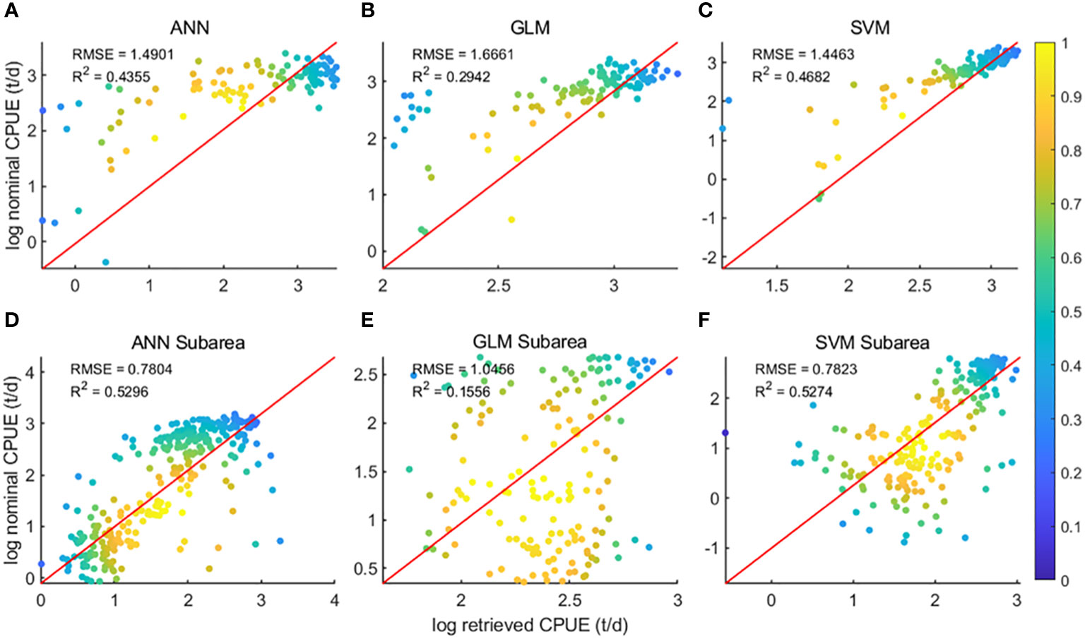
Figure 3 Regression analysis results of the three models; (A–C) is the result of area 48; (D–F) is the result of subarea 48;.

Figure 4 shows the annual and monthly changes in nominal and predicted CPUE using three different models. Of the three methods, the ANN predicts the interannual CPUE trend (Figure 4A) is most consistent with nominal CPUE. The GLM and SVM models predicted similar trends in CPUE, but both were opposite to nominal CPUE. The ANN predicted higher CPUE values, which were on average 100 t/d higher than the nominal CPUE. It basically stayed at 1,000 t/d from 2011-2014, then slightly decreased and stayed around 800 t/d from 2015-2017, reaching a maximum value of 943 t/d in 2019, and then decreased again. The CPUE predicted by the GLM model gradually declined since 2011 and reached a minimum value of 668 t/d in 2014.The CPUE predicted by the SVM model declined from 727 t/d in 2011 year by year till a minimum value of 609 t/d in 2016, and then increased year by year and reached a maximum value in 2020. From the monthly scale change (Figure 4B), the CPUE predicted by the SVM model is the most consistent with the trend of nominal CPUE. The CPUE predicted by the ANN model has a larger difference from the nominal CPUE, with the ANN predicted CPUE being higher than the nominal CPUE by an average of 839 t/d in January to April, and lower than the nominal CPUE by an average of 280 t/d in May to December.

Figure 4

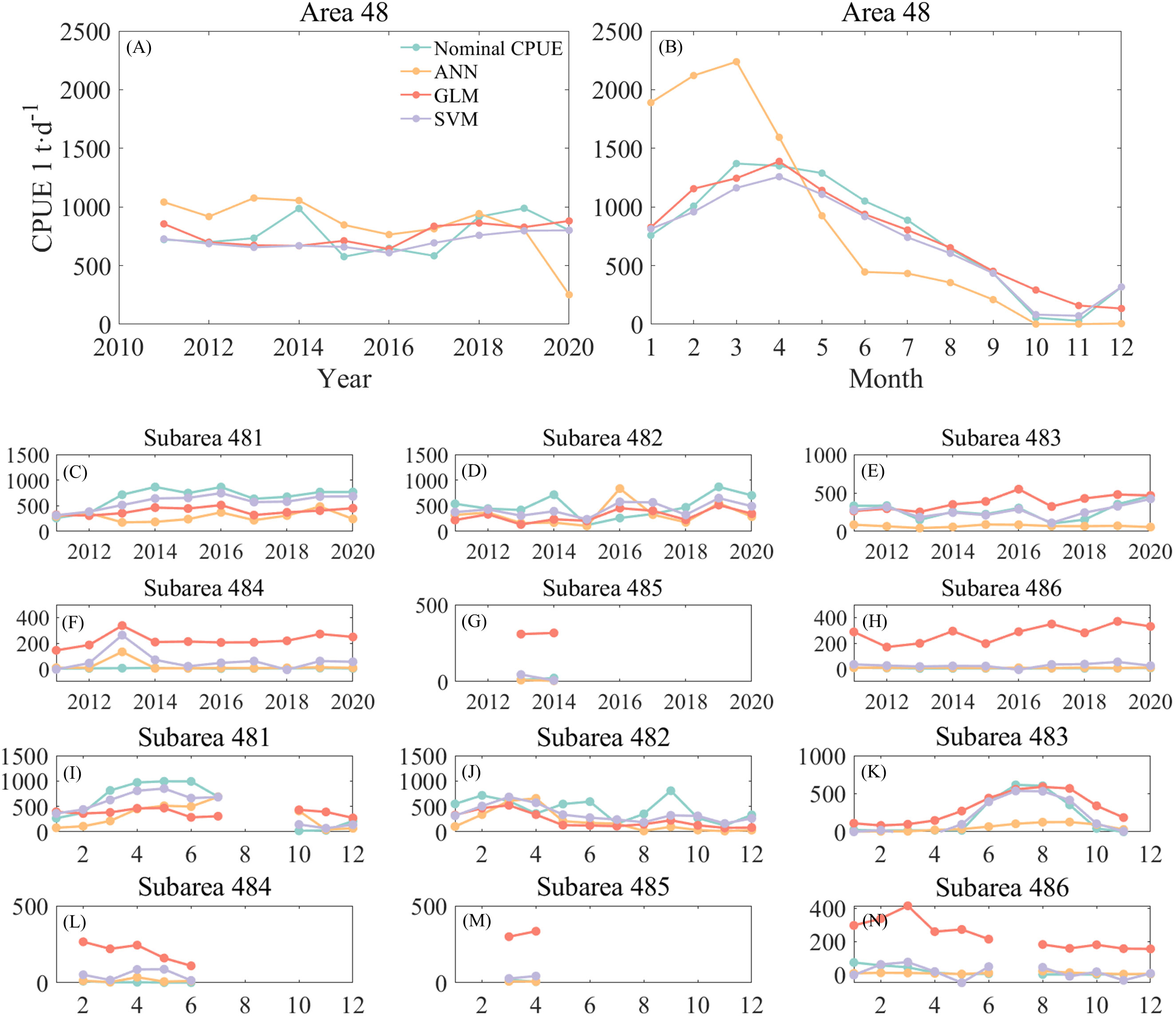
Figure 4 Comparison of annual and monthly changes of CPUE predicted by three models with nominal CPUE: (A) is the annual change of the area 48; (B) is the monthly change of the area 48; (C–H) is the annual change of the subareas, corresponding to 481-486, respectively; (I–N) is the monthly change of the subareas, corresponding to 481-486, respectively.

From the annual scale changes in each subarea (Figures 4C–H), it can be seen that the ANN predicted CPUE lower than the nominal CPUE in subareas 481, 482, and 483, and the predicted CPUE in subareas 484, 485, and 486, had smaller errors from the nominal CPUE. The GLM predicted CPUE significantly higher than the more nominal CPUE in subareas 483 through 486. The gap between CPUE and nominal CPUE predicted by the SVM model is small, but the predicted values of krill in subarea 484 for 2011 and subarea 486 for 2016 are negative. From the monthly scale changes (Figures 4I–N), it can be found that the errors between predicted CPUE and nominal CPUE by the three models are similar to the annual changes. High values of krill CPUE mainly occurred in areas 481, 482 and 483, with CPUE in area 481 increasing month by month from January to the highest value in June. There was no obvious pattern of CPUE change in area 482, with higher CPUE in February and September; high CPUE in area 483 mainly occurred from June to September. Subareas 484 and 485 had fewer months of fishing operations and very low CPUE, while area 486 was a research fishery and CPUE was negative. Subarea 486 is a research fishery and also has low CPUE values. Similar to the annual variation, the SVM predicted negative CPUE in March and April in Area 483 (Figure 4K) and in January, May, September, and November in Area 486 (Figure 4N), so the ANN model was subsequently selected for krill CPUE prediction.

3.2 Predicted results

3.2.1 Results of CALIPSO chlorophyll inversion

Figure 5 shows the distribution of MODIS and CALIPSO CHL in Antarctica in December and June. In December, the CALIPSO diurnal data (Figure 5A) showed significantly higher CHL concentrations in the Argentine Basin and the Mid-Atlantic, Indian Ocean (60°E-90°E, 30°S-50°S), Ross Sea, and South Pacific (150°W-180°W, 55°S-65°S). The distribution is consistent with MODIS (Figure 5C), but the coverage of CALIPSO data is significantly higher in the Antarctic Circle than in MODIS. At night (Figure 5B), CHL concentrations were higher in Atlantic waters (60°W-30°W, 30°S-50°S). In June, MODIS data were missing. The CALIPSO data (Figures 5E, F) showed higher daytime CHL concentrations in the Argentine Basin, with a percentage of daily variation of less than 30%. Within the Antarctic Circle (south of 66°S), nighttime data coverage is higher than daytime.

Figure 5

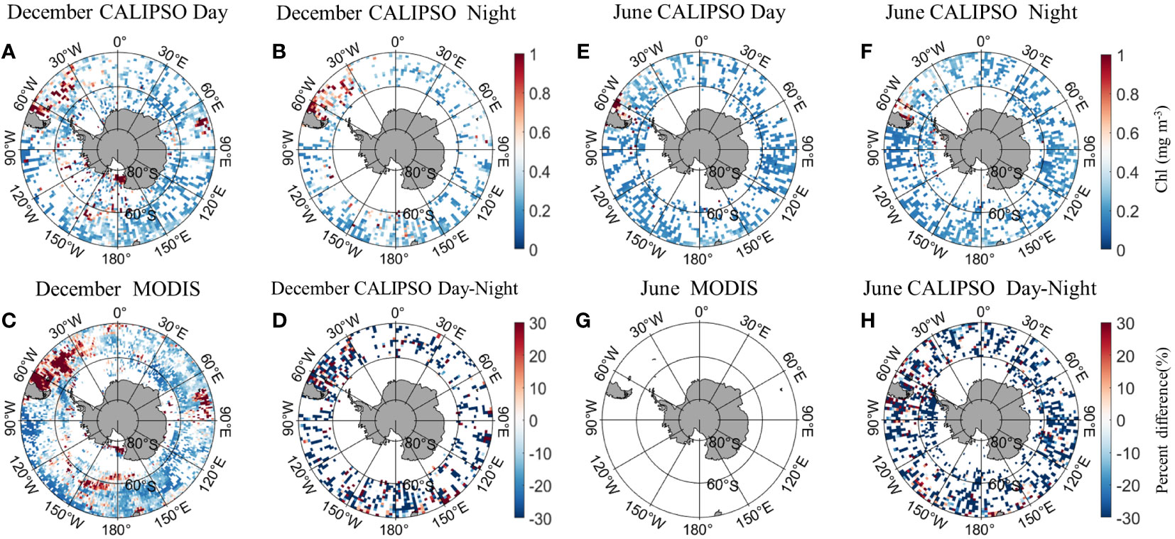
Figure 5 Comparison of active CALIPSO CHL and passive MODIS CHL distribution in the Antarctic. (A) CALIPSO daytime data in December; (B) CALIPSO nighttime data in December; (C) MODIS data in December; (D) percent difference between CALIOP CHL and MODIS CHL in December. (E) CALIPSO daytime data in June; (F) CALIPSO nighttime data in June; (G) MODIS data in June; (H) percent difference between CALIOP CHL and MODIS CHL in June.

3.2.2 Krill CPUE prediction results

Three sets of input data were obtained by matching CALIPSO daytime and nighttime CHL and MODIS CHL data with other environmental factors, respectively, and brought into the ANN model for krill CPUE prediction. Figures 6–8 present the distribution of CPUE predicted by the three sets of data for each month for krill, respectively. It is obvious that MODIS data are missing from May to July (Figures 8E–G), and in the other months, MODIS data have similar distribution and temporal and spatial trends as those predicted using CALIPSO daytime CHL data. This suggests that CALIPSO CHL data can be effective data for predicting krill CPUE and compensate for the lack of MODIS data. There are two main phosphorus aggregations in fishing area 48. A small aggregation located near the Antarctic Peninsula (65°W-45°E, 60°S-66°S) in January, which gradually increases in size and shifts eastward as the months increase (March to May). The size of the aggregation decreased from June onwards and the aggregation disappeared by October. Another large krill aggregation was located in the South Atlantic at 10°W-20°E, 50°S-60°S, which gradually increased in size and concentration and shifted westward as the months changed, with a maximum in March, followed by a gradual decrease in size and finally disappearance of the aggregation in November. Although there are fewer CHL data from June to October, it can still be seen that the center of aggregation of this krill aggregation group is gradually shifting to the northwest, and it can be seen from Figures 6I–K that the aggregation group is finally located mainly in the sea area of 20°W-10°W, 50°S-55°S.

Figure 6

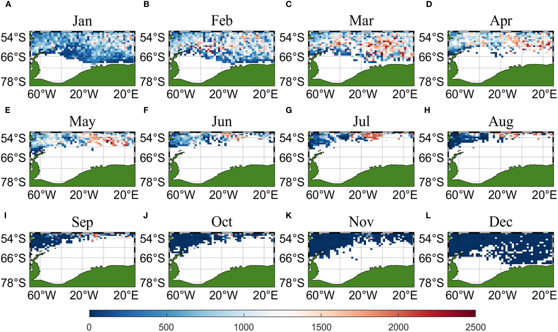
Figure 6 Spatial distribution of climatological monthly Antarctic krill CPUE predicted using daytime CHL data from CALIPSO, with panels (A–L) corresponding to January to December.

Figure 7

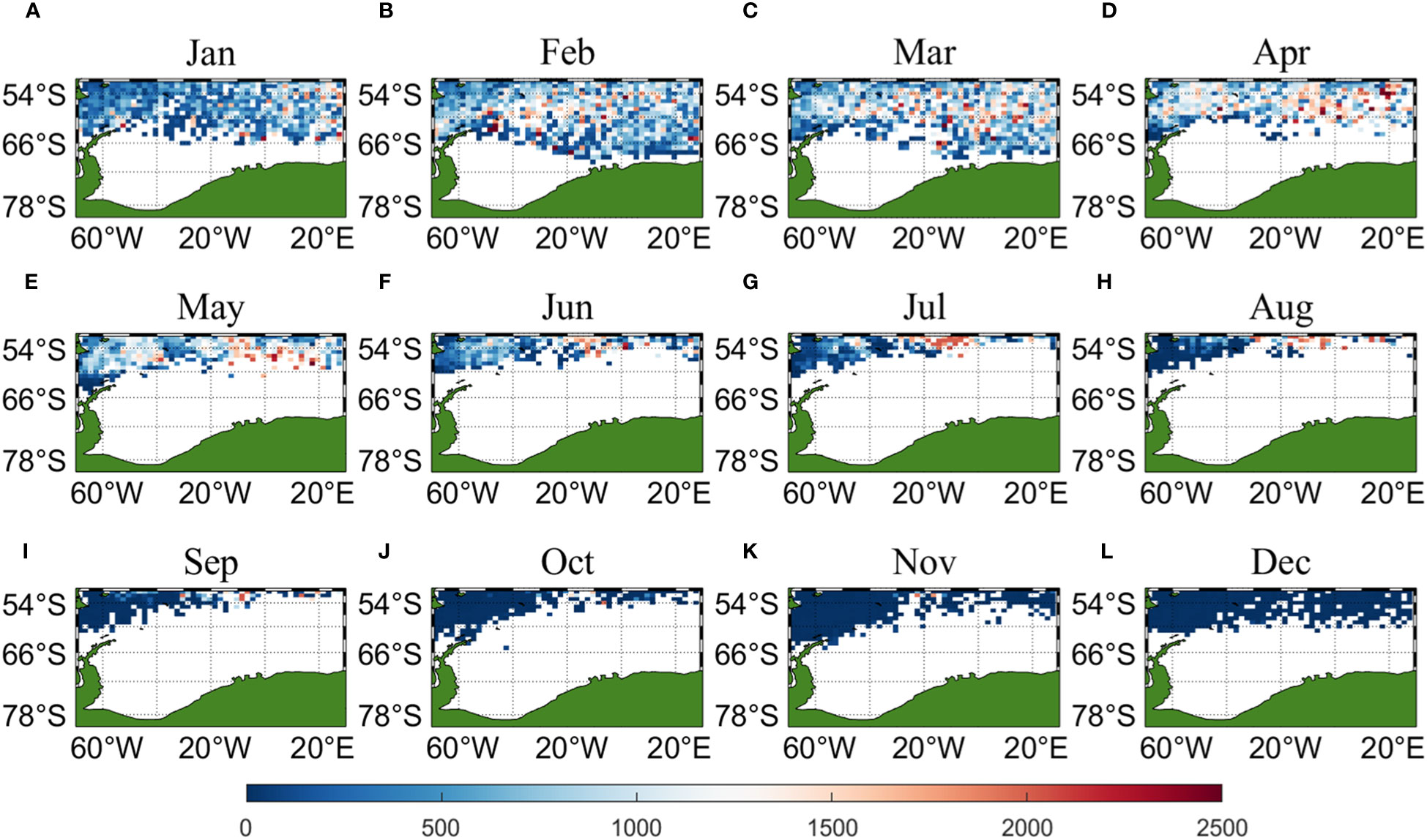
Figure 7 Spatial distribution of climatological monthly Antarctic krill CPUE predicted using nighttime CHL data from CALIPSO, with panels (A–L) corresponding to January to December.

Figure 8

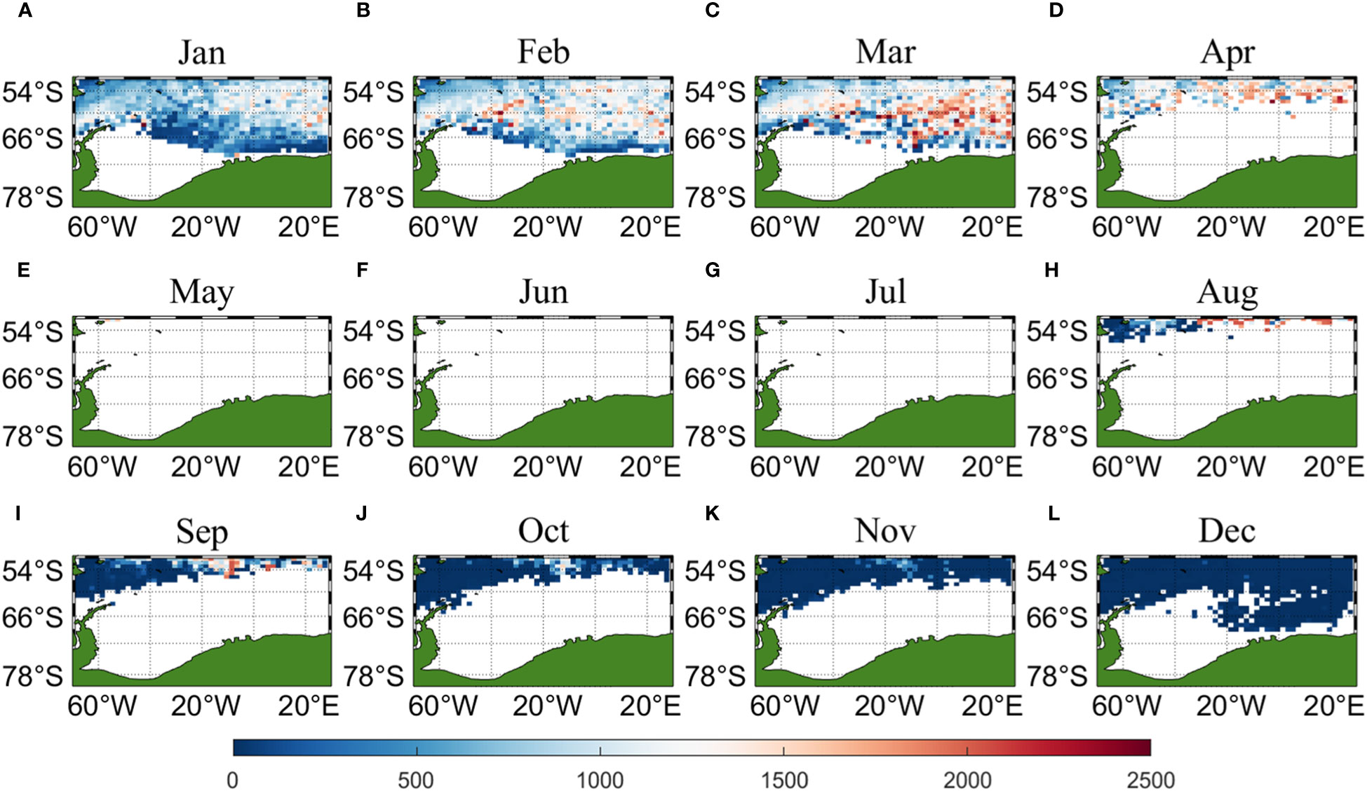
Figure 8 Spatial distribution of climatological monthly Antarctic krill CPUE predicted using CHL data from MODIS, with panels (A–L) corresponding to January to December.

Figure 9 compares the results and significance of CPUE predicted by CALIPSO and MODIS data at different spatial and temporal scales and with different environmental factors. The results show that year has a small effect on CPUE and month has a significant effect on CPUE. Except for 2015 and 2017, the predicted values of CALIPSO data were on average 149 t/d higher than those of MODIS data. Except for June and July, the predicted values of CALIPSO data were on average 102 t/d lower than the predicted values of MODIS data. The high values of CPUE mainly appeared in the months of March to April at about 1000 t/d, and then CPUE decreased significantly with the increase of months. From the spatial distribution, the range of CPUE higher than 500 t/d is concentrated in 67°S-55°S, 20°W-30°E. Among them, the CPUE has a small peak of about 500 t/d at a longitude of 40°W, and then decreases rapidly to 400 t/d, and then increases again, and stays at 700 t/d after reaching a second peak value (about 800 t/d) at about 10°W.

Figure 9

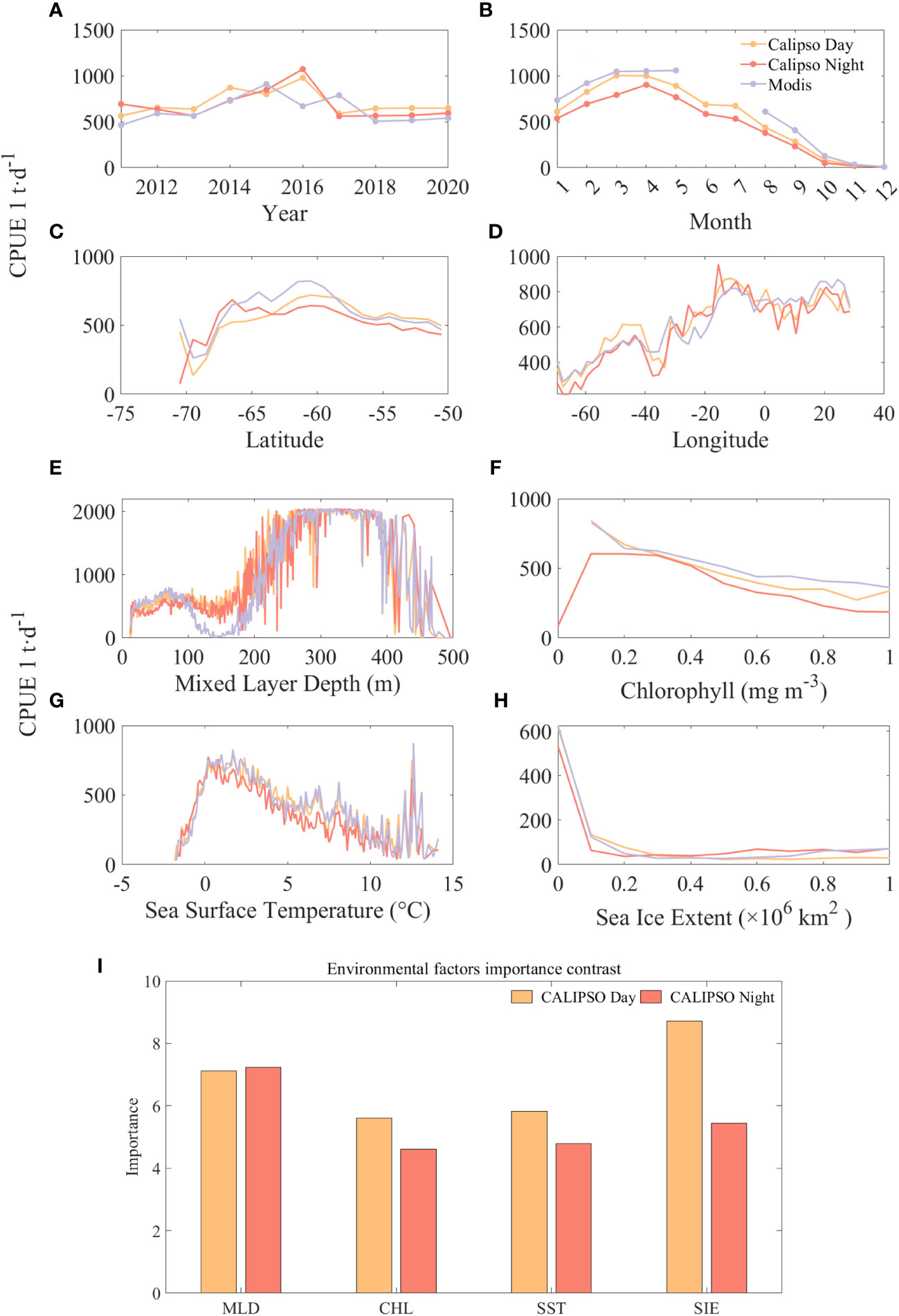
Figure 9 Comparison of the predicted CPUE results from CALIPSO and MODIS data at different spatial and temporal scales and different environmental factors and the band importance contrast: (A) is year; (B) is month; (C) is latitude; (D) is longitude; (E) is MLD, (F) is CHL, (G) is SST, and (H) is SIE, (I) is importance contrast.

Among the four environmental factors, CPUE was higher when MLD and SST were specific ranges and negatively correlated with CHL and SIE. At first, krill CPUE remained around 500 t/d at MLD depths of 0-200 m, then increased rapidly with depth to around 2000 t/d at 270-390 m, and then declined rapidly. Similarly, krill CPUE increased rapidly with SST from -1.7°C to 1.7°C and CPUE increased from 36 t/d to about 750 t/d, followed by a slow decline. For CHL, CPUE was highest at about 800 t/d with CHL of 0.1 mg m^-3, and then decreased to less than 200 t/d when CHL was greater than 1.7 mg m^-3. CPUE was highest at about 600 t/d with SIE of 0, and then only 120 t/d with SIE of 0.1, followed by no significant CPUE with increasing SIE change, keeping at about 50 t/d.

The importance comparison (Figure 9I) reveals the order of importance of the environmental factors, during the daytime the order of importance was: SIE, MLD, SST and CHL. At night MLD turned out to be the most important factor, being 0.1 higher than during the daytime, while SIE decreased by 3.27. This phenomenon can be attributed to the reduced density in stable surface waters in the Antarctic Marginal Sea as ice melts and low-salinity freshwater is injected (Meguro et al., 2004). This reduced density limits vertical mixing and leads to a reduction in the thickness of the mixed layer. Consequently, this favorable condition facilitates extensive phytoplankton colonization of the stable water column, leading to a significant increase in primary productivity (Marrari et al., 2006, 2008). This increase in productivity in turn attracts krill populations to forage.

4 Discussions

4.1 Comparison of ANN, GLM and SVM methods

According to the results of the study, for the subarea data, the CPUE predicted by the GLM was significantly different from the nominal CPUE. The main reason is that the GLM model can only target the expected value of the response variable in a linear relationship with the explanatory variables, while in reality, there is a nonlinear relationship between Antarctic krill CPUE and many factors. In addition GLM has requirements on data structure, and in the presence of outliers or nonlinearities, GLM simulation and prediction errors are larger (Walsh and Kleiber, 2001; Denis et al., 2002). Figure 4 indicates that the difference between the CPUE predicted by SVM and the nominal CPUE trend is much smaller, however, there are negative values of CPUE predicted by the SVM model for the prediction of the subregion 48 data, which may be due to overfitting caused by the parameter settings. The advantages of SVM are good generalization ability, robustness and good performance for high dimensional data and small sample problems. when dealing with large-scale datasets SVM may face the problem of high computational complexity. The predictive performance of SVM models varies widely across studies (Larranaga et al., 2006; Pang et al., 2006), and the selection of the optimal model needs to be determined based on the data type (Verikas et al., 2011).

4.2 Spatial and temporal distribution pattern on CPUE

Antarctic krill CPUE peaked in 2016 and then decreased significantly, and one of the reasons for the decrease in krill populations in 2017 may have been influenced by the 2015/2016 El Niño event. In the report on the state of the global climate in 2015, the World Meteorological Organization (WMO) noted that the 2015 El Niño was one of the three strongest El Niños and the longest El Niño process in the observational record (Zhai et al., 2016). Brown’s study (Brown et al., 2010) on the growth of krill at different temperatures showed that the intermolt period of krill declined significantly with increasing temperature, and that there was a regression of the sexual maturity stage. Tarling et al (Tarling et al., 2006). modeled the prediction of krill growth using factors such as food source, temperature, body length, sex, and sexual maturity, and the result showed that the growth rate of krill decreased with increasing temperature. In addition, changes in the global climate, rising temperatures, melting sea ice, and other changes are exerting some stress on krill maturation, reproduction, and population replenishment. Combining the maps of fishing area distribution (Figure 1B) and the predicted monthly spatial distribution of CPUE for Antarctic krill (Figure 6), it was found that subareas 481 and 482 had higher CPUE in January-April, mainly in the South Shetland Islands (Hewitt et al., 2004), and moved offshore of South Georgia (Comiso and Steffen, 2001) in May-June, thus subarea 483 is higher in May-August and subarea 486 is higher in both January-August.

4.3 Impact of environmental factors on CPUE

There are fewer studies on the relationship between krill CPUE and MLD, but the mixed layer is a vertical mixed layer with almost uniform depth, temperature and salt formed by solar radiation, precipitation and wind (Sun et al., 2007). There have been studies on the relationship between depth and temperature and salt in krill. Hu (Hu et al., 2019) studied the relationship between vertical distribution of Antarctic krill and light, vertical temperature and salt. He pointed out that during the daytime, Antarctic krill were mostly distributed in the 40-120 m water layer, mostly gathered in the thermocline and saline transgression layer, while during the nighttime phase, they were mainly distributed in the two water layers of 20-40 m and 180 m depths, and mostly gathered outside the thermocline and saline transgression layer. Chlorophyll, sea surface temperature and sea ice (Chen et al., 2011) are the main environmental factors affecting the distribution of polar fisheries, and many scholars have investigated the effects of environmental factors on the distribution of Antarctic krill resources. The results of this study showed that the high value of krill CPUE was around 0.1 mg m^-3 at CHL, which is in line with the results of previous studies. Atkinson et al (Atkinson et al., 2008). suggested that CHL in the main habitat of Antarctic krill ranged from 0.5 ~ 1.0 mg/m³, and Zhang et al (Zhang et al., 2020). suggested that the optimal CHL in Antarctica was 0.13 ~ 0.83 mg/m³. Zhu (Zhu, 2012) suggested that high CPUE values usually occur in waters with CHL between 0 ~ 0.2 mg/m³. There is a strong correlation between SST and krill fishery, and seasonal changes in SST lead to spatial and temporal changes in krill fishery. The results of the present study show that the temperature range of high values of CPUE for Antarctic krill is -1.4~5.5°, and the mean annual temperature is 2.57°, which is basically consistent with the results of the previous studies. Zhang’s study (Zhang et al., 2020) on the relationship between CPUE and SST and CHL concentration in the Antarctic krill fishery (fishing area 48) pointed out that the optimum SST of the fishery was -1.8~1.2°C. Dai (Dai et al., 2012) also pointed out in his study that the interannual variation of krill CPUE was highly correlated with SST when SST was 0~1°C (R^{2 =} 0.82). The effect of sea ice on krill CPUE is manifested by the negative correlation between summer krill CPUE and the average sea ice extent in the winter-spring (July-November) of the previous year (Chen et al., 2011). The winter-spring sea ice extent not only affects krill growth, but also influences the timing and extent of Antarctic krill fishing operations, which in turn affects the CPUE of the Antarctic krill fishery.

4.4 Antarctic krill resource assessment

In this study, assessment calculations of krill resources were carried out based on CPUE predicted by CALIPSO diurnal CHL. Figure 10 shows the Antarctic krill biomass from 2011 to 2020, with a general zigzag upward trend in krill biomass. It rises from 2.25 to 2.65 × 10⁸ tons in 2011 to 2.53 to 3.02 × 10⁸ tons in 2020, which is basically in line with the official CCAMLR assessment of krill biomass of 0.6 to 4.2 × 10⁸ tons.

Figure 10

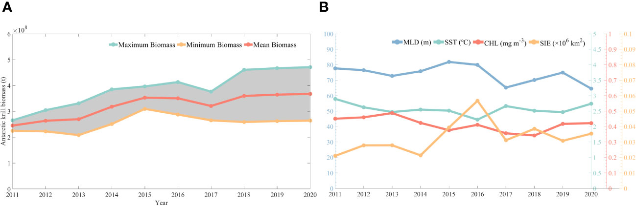
Figure 10 Changes in biological resources of krill (A) and trends in environmental factors (B) from 2011-2020.

The limitations of traditional acoustic assessment are the high cost of the assessment, the need for research vessels or fishing vessels equipped with fishing vessel fish finder collectors for acoustic data collection, and the sea ice cover in some parts of the Antarctic, which limits the range of vessel data collection. In contrast, fishing vessel acoustic imaging contains a large number of abiotic signals and has the disadvantage of being time-consuming and inefficient. Studies using acoustic methods for resource assessment usually focus on the Antarctic Peninsula (subarea 481) and cannot cover the whole 48 fishing areas. For example, based on krill acoustic imaging data, Wang Teng assessed the krill resource in the waters of the South Orkney Islands to be about 4.79×10⁵ t by adopting the traditional integral unit method and a new cluster-based assessment method (Wang, 2018). Dai proposed to hard combine the remote sensing observation data and other environmental factors for in-depth study to improve the interaction between krill resource abundance and environmental factors (Dai et al., 2012).

In this study, resource assessment of the entire 48 fishing areas was realized using satellite-based LiDAR data, demonstrating the feasibility of using active LiDAR for Antarctic krill stock assessment. Active LiDAR can fill in the missing data at high latitudes, with the advantages of high efficiency and high accuracy (Chen et al., 2020) thereby compensating for the high cost and limited assessment range of acoustic assessment. The spatial distribution of krill CPUE reveals that the krill aggregation group in the South Atlantic waters is located in subarea 486, which is currently used only for scientific research and not for commercial fishing, and therefore the Antarctic krill has a large potential biological resource for fishing.

5 Conclusions

In this study, GLM, ANN and SVM models were selected for modeling by combining MLD, CHL, SST and SIE data and Antarctic krill CPUE. The results showed that the ANN and SVM models predicted better results than the GLM, with R² of 0.44 and 0.47, respectively. CALIPSO diurnal and MODIS CHL data were used to bring into the model and the CPUE predictions were compared. The results showed that the data predicted using CALIPSO had a smaller gap with MODIS and were able to effectively fill the data gap of MODIS in polar winters. There was no obvious pattern of interannual variation in krill CPUE; high CPUE values mainly occurred from February to May. Its spatial distribution was in January-April, mainly in the South Shetland Islands, and moved offshore towards South Georgia in May-June. The biomass of Antarctic krill was assessed to increase from 2.25 to 2.65 × 10⁸ tons in 2011 to 2.53 to 3.02 × 10⁸ tons in 2020, which is generally consistent with the official CCAMLR assessment of krill biomass of 0.6 to 4.2 × 10⁸ tons. The use of LiDAR data can effectively work in polar regions and at night, can effectively fill the gap of passive remote sensing, and can realize all-weather uninterrupted detection and inversion of krill biological resources, which can effectively make up for the shortcomings of the high cost of acoustic resource assessment and the need for field detection. In the future, the modeling accuracy of active remote sensing data and CPUE can be further improved to provide more accurate resource assessment data.

Data availability statement

The original contributions presented in the study are included in the article/supplementary material. Further inquiries can be directed to the corresponding author.

Author contributions

CZ: Methodology, Writing – original draft. PC: Conceptualization, Writing – review & editing. ZZ: Data curation, Methodology, Writing – review & editing. CX: Data curation, Validation, Writing – review & editing. SZ: Validation, Writing – review & editing. MS: Data curation, Validation, Writing – review & editing. DW: Data curation, Methodology, Software, Writing – review & editing.

Funding

The author(s) declare financial support was received for the research, authorship, and/or publication of this article. This research was funded by the National Natural Science Foundation (42322606; 42276180; 61991453), the National Key Research and Development Program of China (2022YFB3901703; 2022YFB3902603), the Key Special Project for Introduced Talents Team of Southern Marine Science and Engineering Guangdong Laboratory (GML2021GD0809), the Donghai Laboratory Preresearch project (DH2022ZY0003), and the Key Research and Development Program of Zhejiang Province (grant no. 2020C03100).

Acknowledgments

The authors are grateful to NASA Langley Research Center for providing CALIOP data through the Atmospheric Sciences Data Center (https://asdc.larc.nasa.gov/data/CALIPSO/). We thank the NASA Marine Biology Processing Group and Glob Colour for also providing MODIS products (https://oceandata.sci.gsfc.nasa.gov/). We thank the Commission for the Conservation of Antarctic Marine Living Resources (https://www.ccamlr.org/) for providing Antarctic krill production data. we thank the Copernicus Climate Change Service for providing sea ice data (https://climate.copernicus.eu/sea-ice). we thank the Copernicus Marine Environment Monitoring Service for providing the mixed layer depth data and sea surface temperature data (http://resources.marine.copernicus.eu/product-detail/MULTIOBS_GLO_PHY_TSUV_3D_MYNRT_015_012).We thank reviewers for their suggestions, which significantly improved the presentation of the paper.

Conflict of interest

The authors declare that the research was conducted in the absence of any commercial or financial relationships that could be construed as a potential conflict of interest.

Publisher’s note

All claims expressed in this article are solely those of the authors and do not necessarily represent those of their affiliated organizations, or those of the publisher, the editors and the reviewers. Any product that may be evaluated in this article, or claim that may be made by its manufacturer, is not guaranteed or endorsed by the publisher.

References

Asefa T., Kemblowski M., Mckee M., Khalil A. (2006). Multi-time scale stream flow predictions: The support vector machines approach. J. Hydrol. 318, 7–16. doi: 10.1016/j.jhydrol.2005.06.001.

CrossRef Full Text | Google Scholar

Atkinson A., Siegel V., Pakhomov E., Rothery P., Loeb V., Ross R., et al. (2008). Oceanic circumpolar habitats of Antarctic krill. Mar. Ecol. Prog. Ser. 362, 1–23. doi: 10.3354/meps07498.

CrossRef Full Text | Google Scholar

Behrenfeld M. J., Hu Y., O’malley R. T., Boss E. S., Hostetler C. A., Siegel D. A., et al. (2017). Annual boom–bust cycles of polar phytoplankton biomass revealed by space-based lidar. Nat. Geosci. 10, 118–122. doi: 10.1038/ngeo2861.

CrossRef Full Text | Google Scholar

Bosch P., López J., Ramírez H., Robotham H. (2013). Support vector machine under uncertainty: An application for hydroacoustic classification of fish-schools in Chile. Expert Syst. Appl. 40, 4029–4034. doi: 10.1016/j.eswa.2013.01.006.

CrossRef Full Text | Google Scholar

Brown M., Kawaguchi S., Candy S., Virtue P. (2010). Temperature effects on the growth and maturation of Antarctic krill (Euphausia superba). Deep Sea Res. Part II: Topical Stud. Oceanography 57, 672–682. doi: 10.1016/j.dsr2.2009.10.016

CrossRef Full Text | Google Scholar

Ccamlr (2010). Report of the fifth meeting of the Subgroup on Acoustic Survey and Analysis methods. Report of the fifth meeting of the Subgroup on Acoustic Survey and Analysis methods, 1–25.

Google Scholar

Chen F., Chen X., Liu B., Zhu G., Xu L. (2011). Effect of sea ice on the abundance index of antarctic krill Euphausua Superba. Oceanologia Et Limnologia Sin. 42, 495–499. doi: 10.11693/hyhz201104005005

CrossRef Full Text | Google Scholar

Chen P., Jamet C., Liu D. (2022). LiDAR remote sensing for vertical distribution of seawater optical properties and chlorophyll-a from the east China sea to the south China sea. IEEE Trans. Geosci. Remote Sens. 60, 1–21. doi: 10.1109/TGRS.2022.3174230.

CrossRef Full Text | Google Scholar

Chen P., Mao Z., Zhang Z., Liu H., Pan D. (2020). Detecting subsurface phytoplankton layer in Qiandao Lake using shipborne lidar. Optics express 28 1, 558–569. doi: 10.1364/OE.381617.

CrossRef Full Text | Google Scholar

Chen P., Pan D. (2019). Ocean optical profiling in south China sea using airborne liDAR. Remote Sens. 11, 1826. doi: 10.3390/rs11151826.

CrossRef Full Text | Google Scholar

Clarke A. (1985). “Energy flow in the southern ocean food web,” in Antarctic nutrient cycles and food webs. Eds. Siegfried W. R., Condy P. R., Laws R. M. (Berlin, Heidelberg: Springer), 573–580.

Google Scholar

Comiso J. C., Steffen K. (2001). Studies of Antarctic sea ice concentrations from satellite data and their applications. J. Geophysical Research: Oceans 106, 31361–31385. doi: 10.1029/2001JC000823.

CrossRef Full Text | Google Scholar

Contractor S., Roughan M. (2021). Efficacy of feedforward and LSTM neural networks at predicting and gap filling coastal ocean timeseries: oxygen, nutrients, and temperature. Front. Mar. Sci. 8. doi: 10.3389/fmars.2021.637759.

CrossRef Full Text | Google Scholar

Dai L., Zhang S., Fan W. (2012). The abundance index of antarctic krill and its relationship to sea ice and sea surface temperature. Chin. J. Polar Res. 24, 352–360. doi: 10.3724/SP.J.1084.2012.00352

CrossRef Full Text | Google Scholar

Denis V., Lejeune J., Denis J., Lejeune V., Spatio J., Robin J.-P. (2002). Spatio-temporal analysis of commercial trawler data using General Additive models: patterns of Loliginid squid abundance in the north-east Atlantic. ICES J. Mar. Sci. 59, 633–648. doi: 10.1006/jmsc.2001.1178.

CrossRef Full Text | Google Scholar

Ericson J. A., Hellessey N., Nichols P. D., Kawaguchi S., Nicol S., Hoem N., et al. (2018). Seasonal and interannual variations in the fatty acid composition of adult Euphausia superba Dana 1850 (Euphausiacea) samples derived from the Scotia Sea krill fishery. J. Crustacean Biol. 38, 662–672. doi: 10.1093/jcbiol/ruy032.

CrossRef Full Text | Google Scholar

Guoqin Z., Junrong L., Fenghua T., Wei F., Xuefeng S., Yang C., et al. (2022). Temporal and spatial distribution of antarctic krill in 48 fishing areas based on fishery data. Prog. Fishery Sci. 43, 81–92. doi: 10.19663/j.issn2095—9869.20210407004

CrossRef Full Text | Google Scholar

Hampton I. (1985). “Abundance, distribution and behaviour of euphausia superba in the southern ocean between 15° and 30° E during FIBEX,” in Antarctic nutrient cycles and food webs. Eds. Siegfried W. R., Condy P. R., Laws R. M. (Berlin, Heidelberg: Springer), 294–303. doi: 10.1007/978-3-642-82275-9_42

CrossRef Full Text | Google Scholar

Hewitt R., Watkins J., Naganobu M., Sushin V., Brierley A., Demer D., et al. (2004). Biomass of Antarctic krill in the Scotia Sea in January/February 2000 and its use in revising an estimate of precautionary yield. Deep Sea Res. Part II: Topical Stud. Oceanography 51, 1215–1236. doi: 10.1016/S0967-0645(04)00076-1.

CrossRef Full Text | Google Scholar

Hu S., Xu L., Wang T., Tang H., Zhou C., Zhu G. (2019). Vertical distribution of Euphausia Superba in sea areas around the South Orkney Islands in autumn 2017 and its relations with illumination,vertical temperature and salinity. Mar. Fisheries 41, 160–168. doi: 10.13233/j.cnki.mar.fish.2019.02.004

CrossRef Full Text | Google Scholar

Hua C., Zhu Q., Shi C., Liu Y. (2019). Comparative analysis of CPUE standardization of Chinese pacific saury (Cololabis saira) fishery based on GLM and GAM. Acta Oceanologica Sin. 38 (10), 100–110. doi: 10.1007/s13131-019-1486-3

CrossRef Full Text | Google Scholar

Larranaga P., Calvo B., Santana R., Bielza C., Galdiano J., Inza I., et al. (2006). Machine learning in bioinformatics. Briefings Bioinf. 7, 86–112. doi: 10.1093/bib/bbk007.

CrossRef Full Text | Google Scholar

Laws R. M. (1985). The ecology of the southern ocean. Am. Scientist 73, 26–40.

Google Scholar

Li Z. L., Huang H. L., Qu T. C., Yang Q., Chen S., Liu J., et al. (2015). A correlation study between the marine environment and the spatial-temporal distribution of Antarctic krill(Euphausia superba Dana) in Prydz Bay. J. Fishery Sci. China 22, 488–500. doi: 10.3724/SP.J.1118.2015.14474

CrossRef Full Text | Google Scholar

Li S., Yang J., Zhao G., Li L., Rao X., Hongliang H. (2022). Spatial distribution of Antarctic krill and their relationship with chlorophyll concentration in the Amundsen Sea in summer. Chin. J. Polar Res. 34, 451–459. doi: 10.13679/j.jdyj.20210075

CrossRef Full Text | Google Scholar

Liu H., Chen P., Mao Z. H., Pan D. L., He Y. (2018). Subsurface plankton layers observed from airborne lidar in Sanya Bay, South China Sea. Optics Express 26, 29134–29147. doi: 10.1364/OE.26.029134.

PubMed Abstract | CrossRef Full Text | Google Scholar

Liu X., Wang L., Yang J., Deng K. (2015). Competitiveness analysis for China7S ocean acoustic detection technologies. J. Ocean Technol. 34, 80–85.

Google Scholar

Lu X. M., Hu Y. X., Trepte C., Zeng S., Churnside J. (2014). Ocean subsurface studies with the CALIPSO spaceborne lidar. J. Geophysical Research: Oceans 119, 4305–4317. doi: 10.1002/2014JC009970.

CrossRef Full Text | Google Scholar

Lu X., Hu Y., Yang Y., Neumann T., Omar A., Baize R., et al. (2021). New ocean subsurface optical properties from space lidars: CALIOP/CALIPSO and ATLAS/ICESat-2. Earth Space Sci. 8, e2021EA001839. doi: 10.1029/2021EA001839.

CrossRef Full Text | Google Scholar

Maier H. R., Dandy G. C. (2001). Neural network based modelling of environmental variables: A systematic approach. Math. Comput. Model. 33, 669–682. doi: 10.1016/S0895-7177(00)00271-5.

CrossRef Full Text | Google Scholar

Marrari M., Daly K. L., Hu C. (2008). Spatial and temporal variability of SeaWiFS chlorophyll a distributions west of the Antarctic Peninsula: Implications for krill production. Deep Sea Res. Part II: Topical Stud. Oceanography 55, 377–392. doi: 10.1016/j.dsr2.2007.11.011.

CrossRef Full Text | Google Scholar

Marrari M., Hu C., Daly K. (2006). Validation of SeaWiFS chlorophyll a concentrations in the Southern Ocean: A revisit. Remote Sens. Environ. 105, 367–375. doi: 10.1016/j.rse.2006.07.008.

CrossRef Full Text | Google Scholar

Meguro H., Toba Y., Murakami H., Kimura N. (2004). Simultaneous remote sensing of chlorophyll, sea ice and sea surface temperature in the Antarctic waters with special reference to the primary production from ice algae. Adv. Space Res. 33, 1168–1172. doi: 10.1016/S0273-1177(03)00368-5.

CrossRef Full Text | Google Scholar

Morris C. W., Autret A., Boddy L. (2001). Support vector machines for identifying organisms — a comparison with strongly partitioned radial basis function networks. Ecol. Model. 146, 57–67. doi: 10.1016/S0304-3800(01)00296-4.

CrossRef Full Text | Google Scholar

Nicol S., Foster J. (2003). Recent trends in the fishery for Antarctic krill. Aquat. Living Resour. 16, 42–45. doi: 10.1016/S0990-7440(03)00004-4.

CrossRef Full Text | Google Scholar

Nicol S., Worby A. P., Leaper R. (2008). Changes in the Antarctic sea ice ecosystem: potential effects on krill and baleen whales. Mar. Freshw. Res. 59, 361–382. doi: 10.1071/MF07161.

CrossRef Full Text | Google Scholar

Pang H., Lin A., Holford M., Enerson B., Lu B., Lawton M., et al. (2006). Pathway analysis using random forests classification and regression. Bioinf. (Oxford England) 22, 2028–2036. doi: 10.1093/bioinformatics/btl344.

CrossRef Full Text | Google Scholar

Renhe Z. (1994). Advances in marine acoustics research in China. Physical 23, 513–518.

Google Scholar

Rifaldi M., Setiawan E. (2019). Competence classification of twitter users using support vector machine (SVM) method (Kuala Lumpur: 2019 7th International Conference on Information and Communication Technology (ICoICT)).

Google Scholar

Rodríguez-Marín E., Arrizabalaga H., Ortiz M., Rodríguez-Cabello C., Moreno G., Kell L. (2003). Standardization of bluefin tuna, Thunnus thynnus, catch per unit effort in the baitboat fishery of the Bay of Biscay (Eastern Atlantic). ICES J. Mar. Sci. 60, 1216–1231. doi: 10.1016/S1054-3139(03)00139-5.

CrossRef Full Text | Google Scholar

Sadeghi M., Asanjan A. A., Faridzad M., Nguyen P., Hsu K., Sorooshian S., et al. (2019). PERSIANN-CNN: precipitation estimation from remotely sensed information using artificial neural networks–convolutional neural networks. J. Hydrometeorol. 20, 2273–2289. doi: 10.1175/JHM-D-19-0110.1.

CrossRef Full Text | Google Scholar

Santa Cruz F., Ernst B., Arata J. A., Parada C. (2018). Spatial and temporal dynamics of the Antarctic krill fishery in fishing hotspots in the Bransfield Strait and South Shetland Islands. Fisheries Res. 208, 157–166. doi: 10.1016/j.fishres.2018.07.020.

CrossRef Full Text | Google Scholar

Sharma S., Sharma S., Athaiya A. (2020). Activation functions in neural networks. Int. J. Eng. Appl. Sci. Technol. 04, 310–316. doi: 10.33564/IJEAST.2020.v04i12.054.

CrossRef Full Text | Google Scholar

Siegel V. (2005). Distribution and population dynamics of Euphausia superba: summary of recent findings. Polar Biol. 29, 1–22. doi: 10.1007/s00300-005-0058-5.

CrossRef Full Text | Google Scholar

Siege V., Damm U., Sushin V. A. (1998). Catch per unit effort (Cpue) data from the early years of commercial krill fishing operations in the atlantic sector of the Antarctic. CCAMLR Sci. 5, 31–50.

Google Scholar

Stowasser G., Atkinson A., Mcgill R., Phillips R. A., Collins M. A., Pond D. W. (2012). Food web dynamics in the Scotia Sea in summer: A stable isotope study. Deep Sea Res. Part II: Topical Stud. Oceanography 59-60, 208–221. doi: 10.1016/j.dsr2.2011.08.004.

CrossRef Full Text | Google Scholar

Sullivan J. M., Donaghay P. L., Rines J. E. B. (2010). Coastal thin layer dynamics: Consequences to biology and optics. Continental Shelf Res. 30, 50–65. doi: 10.1016/j.csr.2009.07.009.

CrossRef Full Text | Google Scholar

Sun Z., Liu L., Yu W. (2007). Study on seasonal variations in the Tropical Indian Ocean Mixed Layer Depth Derived From Argo Float Data. Adv. Mar. Sci. 25, 280–288. doi: 10.3969/j.issn.1671-6647.2007.03.004

CrossRef Full Text | Google Scholar

Suryanarayana I., Braibanti A., Sambasiva Rao R., Ramam V. A., Sudarsan D., Nageswara Rao G. (2008). Neural networks in fisheries research. Fisheries Res. 92, 115–139. doi: 10.1016/j.fishres.2008.01.012.

CrossRef Full Text | Google Scholar

Tarling G. A., Shreeve R. S., Hirst A. G., Atkinson A., Pond D. W., Murphy E. J., et al. (2006). Natural growth rates in Antarctic krill (Euphausia superba): I. Improving methodology and predicting intermolt period. Limnol. Oceanogr. 51, 959–972. doi: 10.4319/lo.2006.51.2.0959.

CrossRef Full Text | Google Scholar

Verikas A., Gelzinis A., Bacauskiene M. (2011). Mining data with random forests: A survey and results of new tests. Pattern Recognition 44, 330–349. doi: 10.1016/j.patcog.2010.08.011.

CrossRef Full Text | Google Scholar

Walsh W., Kleiber P. (2001). Generalized additive model and regression tree analysis of blue shark (Prionace glauca) by the Hawaii-based longline fishery. Fisheries Res. 53, 115–131. doi: 10.1016/S0165-7836(00)00306-4.

CrossRef Full Text | Google Scholar

Wang T. (2018). Acoustic estimate of Antarctic krill in the South Orkney Islands (Shanghai, Chica: Shanghai Ocean University).

Google Scholar

Yang S., Dai Y., Fan W., Shi H. (2020). Standardizing catch per unit effort by machine learning techniques in longline fisheries: a case study of bigeye tuna in the Atlantic Ocean. Ocean Coast. Res. 68, 83–93. doi: 10.1590/s2675-28242020068226.

CrossRef Full Text | Google Scholar

Yang Y., Pan H., Zheng D., Zhao H., Zhou Y., Liu D. (2022). Characteristics and formation conditions of thin phytoplankton layers in the northern gulf of Mexico revealed by airborne lidar. Remote Sens. 14, 4179. doi: 10.3390/rs14174179.

CrossRef Full Text | Google Scholar

Yang S. L., Zhang Y., Zhang H., Fan W. (2015). Comparison and analysis of different model algorithms for CPUE standardization in fishery. Trans. Chin. Soc. Agric. Eng. 31, 259–264. doi: 10.11975/j.issn.1002-6819.2015.21.034

CrossRef Full Text | Google Scholar

Yang Y., Zhu G. P. (2018). Assessment on marine living resources based on acoustic technology and its application in Antarctic krill abundance estimation. Mar. Fisheries 40. doi: 10.13233/j.cnki.mar.fish.2018.03.013

CrossRef Full Text | Google Scholar

Yoshitomi B., Oshima S., Takahashi M. (2007). Multi-dimensional utilization of marine biomass resource: antarctic krill (Enphausia superba Dana). kuroshio Sci. 1, 56–71.

Google Scholar

Yunfeng W., Tian Y., Rencheng Y., Qingchun Z., Fanzhou K., Mingjiang Z. (2020). Research progresses of thin phytoplankton layer in the ocean. Mar. Sci. 44, 86–95. doi: 10.11759/hykx20200120004

CrossRef Full Text | Google Scholar

Zan H., Chen H., Hsu C. J., Chen W. H., Wu S. (2004). Credit rating analysis with support vector machines and neural networks: a market comparative study. Decision Support Systems. 37, 543–558. doi: 10.1016/S0167-9236(03)00086-1

CrossRef Full Text | Google Scholar

Zhai P., Yu R., Guo Y., Li Q., Ren X., Wang Y., et al. (2016). The strong El Niño process in 2015/2016 and its main impacts on global and Chinese climate. Acta meteorokogica Sin. 74, 309–321. doi: 10.11676/qxxb2016.04

CrossRef Full Text | Google Scholar

Zhang S., Chen P. (2022). Subsurface phytoplankton vertical structure from lidar observation during SCS summer monsoon onset. Opt Express 30, 17665–17679. doi: 10.1364/OE.453094.

PubMed Abstract | CrossRef Full Text | Google Scholar

Zhang Z., Chen P., Zhong C., Xie C., Sun M., Zhang S., et al. (2023). Chlorophyll and POC in polar regions derived from spaceborne lidar. Front. Mar. Sci. 10. doi: 10.3389/fmars.2023.1050087.

CrossRef Full Text | Google Scholar

Zhang Y. Y., Xu B., Zhang H., Cheng T. F., Yang S. L. (2020). Interannual and monthly variations of catch per unit effort and the relation with sea surface temperature and chlorophyll concentration in fishing grounds (fishing area 48) of Antarctic krill. Chin. J. Ecol. 39, 1685–1694. doi: 10.13292/j.1000-489.20200.034

CrossRef Full Text | Google Scholar

Zhu G. P. (2012). Effects of temporal and environmental factors on the fishing ground of Antarctic krill (Euphausia superba) in the northern Antarctic Peninsula based on generalized additive model. J. Fisheries China 36, 1863–1871. doi: 10.3724/SP.J.1231.2012.27709.

CrossRef Full Text | Google Scholar