Intrathermocline eddies observed in the northwestern subtropical Pacific Ocean

1 Introduction

Intrathermocline eddies (ITEs) are a special class of oceanic eddies that have their cores or maximum velocities between the seasonal and permanent thermoclines. Like surface mesoscale eddies, ITEs can also be divided into aniticyclonic and cyclonic types. Anticyclonic ITEs show a lens-like thermocline structure with a dome shape in the upper layers and a bowl shape in the lower layers (Gordon et al., 2002; Zhang et al., 2015; Assassi et al., 2016), while cyclonic ITEs show bowl-shaped isopleths in the shallower levels and dome-shaped isopleths in the deeper levels, with the shape termed as “thinny” (McGillicuddy, 2015). Compared to surface-intensified eddies, ITEs play a greater role in the distribution of heat, salt and water masses in the intermediate and deeper parts of the ocean (Tréguier et al., 2012; Hormazabal et al., 2013). In addition, Hansen et al. (2010) suggested that there was an evidence of phytoplankton being advected toward the center of the eddies, but also of isolated phytoplankton blooms within the ITEs based on satellite observations.

Some ITEs display signals at the sea surface (Dilmahamod et al., 2018) like the surface eddies, while others do not (Lin et al., 2017). ITEs are usually discovered through observations from hydrographic surveys and the uneven spatial distribution of Argo data. There are also methodologies designed to detect ITEs from the combination of satellite altimeter data and Argo data (Dilmahamod et al., 2018). In recent decades, despite the difficulties in observation compared to surface eddies, ITEs have been detected in many parts of the world ocean, such as the South China Sea (Zhang et al., 2014; Lin et al., 2017; Qi et al., 2022; Zhang et al., 2022), the Bay of Bengal (Gordon et al., 2017; Jithin and Francis, 2021; Zhou et al., 2022), the Eastern Equatorial Indian Ocean (Hu et al., 2022), the Southern Indian Ocean (Nauw et al., 2006; Dilmahamod et al., 2018), the Japan Sea (Gordon et al., 2002; Ou and Gordon, 2002; Hogan and Hurlburt, 2006), the Northwest Pacific Ocean (Nan et al., 2017; Xu et al., 2017; Ding et al., 2022), the Peru-Chile Undercurrent Zone (Thomsen et al., 2016) and the region of the Gulf Stream (Gula et al., 2019).

Previous studies suggest that possible generation mechanisms of ITEs include flow separation (Thomsen et al., 2016), subduction of surface water (Spall, 1995; Ou and Gordon, 2002), subduction of mode water (Takikawa et al., 2005; Nan et al., 2017), eddy-wind interactions (McGillicuddy, 2015; Gordon et al., 2017), potential vorticity (PV) reduction at wind-forced fronts (Thomas, 2008), changes in upper ocean stratification (He et al., 2020) and undercurrent instability (Combes et al., 2015). For example, subduction of surface mixed-layer water associated with baroclinic instability at frontal convergence could cause the generation of ITEs (Spall, 1995; Ou and Gordon, 2002). McGillicuddy (2015) proposed that eddy-wind interactions may drive a local upwelling that induces doming of isopycnals in anticyclonic eddies. Gordon et al. (2017) detected an ITE in the Bay of Bengal and found that it was transformed from a surface anticyclonic eddy under the impact of a tropical cyclone. Thomas (2008) suggested that a reduction in PV due to winds at oceanic fronts could also lead to the formation of ITEs in the ocean.

Statistical descriptions of eddy activities based on satellite altimetry observations reveal that the northwestern Pacific Ocean is a region with a high probability of surface eddy occurrence, especially in the Kuroshio Extension (KE) region and the Subtropical Countercurrent zonal band (Qiu and Chen, 2013; Yang et al., 2013). On the other hand, sporadic in situ observations have shown evidence that subsurface-intensified eddies also exist in this region. Several ITEs were observed in the northwestern Pacific Ocean, and the North Pacific Subtropical Mode Water (STMW) was usually found in their cores. For example, a subsurface anticyclonic eddy (SAE) was detected southeast of the Ryukyu Islands in February 2002 by Takikawa et al. (2005). The lens-shaped structure of the eddy was located approximately between 150-450 m. The thickness and width of the eddy were approximately 300 m and 100 km, respectively. The water mass in the eddy core was characterized as the STMW. Nan et al. (2017) detected an extra-large SAE with a horizontal scale of 470 km in the Northwest Pacific subtropical gyre in October 2014. Their analysis indicated that the SAE formed in the STMW region and then propagated westward for over 1500 km. Based on enhanced eddy-tracking observations, Xu et al. (2017) captured two anticyclonic eddies south of the KE and found that both eddies were characterized by a lens-shaped thermocline encompassing thick STMW. Based on SLA images and Argo observations, Ding et al. (2022) reported a long-standing SAE south of Japan. The vertical structure, evolutionary process and biogeochemical characteristics of this eddy were also investigated. In addition, subthermocline eddies, as another kind of subsurface-intensified eddy characterized by having their cores below the permanent thermocline, were also observed in the northwestern Pacific Ocean (Oka et al., 2009; Zhang et al., 2015; Zhu et al., 2021).

Based on the outputs of the Oceanic General Circulation Model for the Earth Simulator (OFES), the characteristics of subsurface eddies (SSEs) in the northwestern Pacific Ocean such as distribution, size, amplitude, polarity and longevity were investigated by Xu et al. (2019). The latitudinal band between 9°N and 17°N, the KE region and the area east of the Ryukyu Islands were found to have high probability of SSE occurrence. Interestingly, few SSEs were found within the Subtropical Countercurrent zonal band while surface eddies were widely distributed there.

In this study, we reported two ITEs in the northwestern subtropical Pacific Ocean from underwater glider observations during August-October 2019. The vertical structure, thermohaline properties, evolutionary process, generation mechanisms and energy source of these two ITEs were also examined in detail based on Argo observations, satellite altimeter data and an ocean reanalysis product. The rest of this paper is organized as follows. The datasets used in this study are described in Section 2. The general characteristics and evolutionary process of these two ITEs are provided in Section 3. Section 4 discusses possible generation mechanisms and energy source of these two ITEs. Section 5 presents our conclusion.

2 Data

2.1 Underwater glider data

A research cruise was conducted in the northwestern subtropical Pacific Ocean (145-180°E, 15-30°N) from 13 August to 7 November, 2019. The goal of the cruise was to investigate the marine environment variation and air‐sea interaction in the northwestern Pacific Ocean. During the cruise, comprehensive observations consisting of hydrographic observations, buoy and mooring measurements were conducted. In addition, a Sea-Wing underwater glider, designed by the Shenyang Institute of Automation, Chinese Academy of Sciences (Yu et al., 2011), was deployed at P1 (158°E, 25°N) on 25 August 2019 and recovered at P7 (164.67°E, 27°N) on 10 October 2019 during the cruise to collect hydrographic data in the northwestern subtropical Pacific Ocean.

The glider observation region was located south of the KE. During the glider observation period (August-October, 2019), the KE exhibited a small meander path between 141-153°E and a much larger meander path east of 153°E (Figure 1), which might favor the eddy generation.

Figure 1

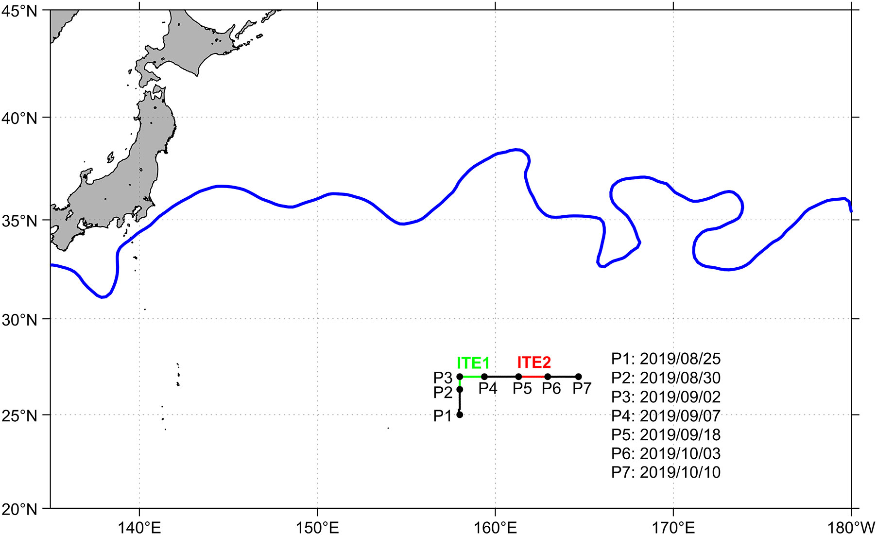
Figure 1 Geographic location of the study area. The glider track is shown as black line. Different points (P1-P7) are marked as black solid circles along the glider track (transect P). The position of ITE1 (ITE2) observed by the glider is colored in green (red).The blue line is the 100 cm Absolute Dynamic Topography (ADT) contour averaged in August-October 2019, representing the Kuroshio Extension jet axis.

Tracks of the glider are shown in Figure 1. Temperature, salinity and pressure were measured by a Seabird CTD installed on the glider. It took about 2 hours for the glider to finish one sampling cycle (0 - 500 m), with the sensor sampling interval of 6 seconds. Temperature and salinity data were then interpolated into 1 m vertical interval. In this study, two ITEs (ITE1 and ITE2) in the northwestern subtropical Pacific Ocean were detected by the glider in August-October 2019. The locations of the glider temperature/salinity (T/S) profiles used in this study are shown as blue dots in Figure 2D.

Figure 2

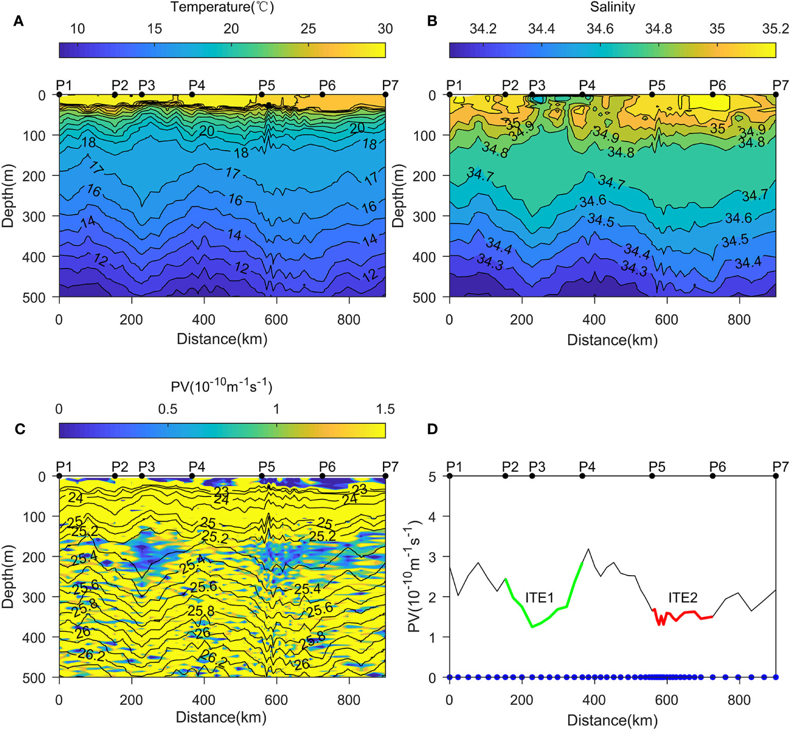
Figure 2 Vertical distributions of (A) temperature (°C), (B) salinity, (C) potential density (kg/m³, contours), PV (10^-10m^-1s^-1, shading) and (D) 25.0-25.4σ_θ averaged PV variation along transect P based on glider observations. In (D), the PV variation within ITE1 (ITE2) is colored in green (red), and the locations of glider profiles used in this study are shown as blue dots.

2.2 Argo data

Temperature and salinity profiles from two Argo floats (ID: 2903424 and 2903427) were obtained from the China Argo Real-Time Data Center (http://www.argo.org.cn). Twelve T/S profiles from Argo2903424 (June-September 2019) and twelve T/S profiles from Argo2903427 (October 2019- February 2020) were used in this study to further investigate the structure of ITE2. The China Argo Real-Time Data Center conducted quality control of the Argo data used in this study.

2.3 Satellite data

The satellite data used in this study include sea level anomaly (SLA) and the Mesoscale Eddy Trajectory Atlas (META) 2.0 DT dataset. Daily SLA were used to present surface signals in the study area. The daily SLA data at 1/4° × 1/4° resolution were released by the Copernicus Marine Environment Monitoring Service (CMEMS, http://marine.copernicus.eu/). The Mesoscale Eddy Trajectory Atlas (META) 2.0 DT is an altimetry-based global dataset of eddy trajectories and properties, from January 1993 to March 2020, distributed by Archiving, Validation and Interpretation of Satellite Oceanographic Data+ (AVISO, https://www.aviso.altimetry.fr/en/data/products/). The data processing methods used in constructing this dataset are described in detail elsewhere (Chelton et al., 2011). This dataset was used to display the track, position and radius of an anticyclonic eddy (AE2) in this study.

2.4 Reanalysis data

The reanalysis data used in this study is the Global Ocean Physics Reanalysis (GLOBAL_MULTIYEAR_PHY_001_030) distributed by the CMEMS. This dataset, termed CMEMS reanalysis for brevity, has a horizontal resolution of 1/12° in both longitude and latitude, 50 vertical levels ranging from 0 to 5700 m, including 31 levels in the upper 500 m. The CMEMS reanalysis is based on the current real-time global forecasting CMEMS system and has assimilated altimeter data (SLA), satellite SST, sea ice concentration, and vertical in situ temperature and salinity profiles. This dataset is in good agreement with the observations and has been widely used for the study of oceanic mesoscale eddies (e.g., Lin et al., 2017; Qian et al., 2018). The daily temperature and salinity data from this dataset were used to investigate the structure, evolution and dynamics of the observed ITEs in this study.

2.5 WOA18 data

The World Ocean Atlas 2018 (WOA18) monthly climatological temperature and salinity data with a spatial resolution of 0.25° × 0.25° (http://apdrc.soest.hawaii.edu/data/data.php) were used to present the climatological mean thermohaline properties in the glider observation region and its adjacent area.

3 Results

3.1 Vertical structure of two ITEs from underwater glider observations

Vertical distributions of T, S and potential density (σ_θ) along the glider track (transect P) are shown in Figures 2A–C. The observations present a peculiar feature in the T distribution: the isotherms formed dome-shaped structures in the upper part of the thermocline (40-170 m) and bowl-shaped structures in 170-500 m between P2-P4 and P5-P6. These two lens-shaped thermal structures with their cores located at ~170 m indicate the presence of typical anticyclonic ITEs (hereafter ITE1 and ITE2). The lens-shaped structures can also be seen from the vertical distribution of σ_θ. Similar changes in isohalines were only present below 70 m, and the isohalines above 70 m did not show obvious shoaling signs as the isotherms did. Notably, there was a patch of low-salinity water at 0-50 m between P3-P4 (Figure 2B), obviously different from the ambient waters.

The lens-shaped structure of ITE1 was clearly evident. According to the glider track (Figure 1) and the feature of the lens-shaped structure between P2-P4 (Figures 2A-C), we infer that P3 was probably located within the core of ITE1 and P2 (P4) was located at the southern (eastern) edge of ITE1. In contrast, the lens-shaped structure of ITE2 was less prominent. In our opinion, it might be the case that the glider just crossed ITE2 without entering its core.

The potential vorticity (PV) was also calculated along transect P, which is defined as:

$$\text{PV=}-\frac{\text{f }}{{\text{σ}}_{\text{θ}}}\frac{\partial {\text{σ}}_{\text{θ}}}{\partial \text{z}},$$

where f is the Coriolis parameter, σ_θ is potential density and $\frac{\partial {\text{σ}}_{\text{θ}}}{\partial \text{z}}$ is the vertical gradient of potential density. As shown in Figure 2C, low PV water was found in the mixed layer and also in the area where the two observed lens-shaped structures were situated, which resulted primarily from weak stratification, in agreement with the vertical distributions of T, S and σ_θ.

Previous studies suggest that the North Pacific Subtropical Mode Water (STMW), which forms south of the KE and is characterized as low PV water (PV< 2×10^-10m^-1s^-1) within the main thermocline (Hanawa, 1987), can be trapped inside ITEs (Nan et al., 2017; Xu et al., 2017). The STMW was also found within ITE1 and ITE2 with the lowest PV located at 25.0-25.4σ_θ between P2-P4 and P5-P6 (Figure 2C). Figure 2D shows the time series of PV averaged vertically in the STMW density layer (25.0-25.4σ_θ) along transect P. The PV inside ITE1 (between P2-P4, green line) decreased gradually, reached its minimum at P3 on 2 September 2019 and then increased again, while the PV inside ITE2 remained roughly unchanged between P5-P6 (red line). This indicates different dynamics for the two ITEs and will be discussed in Section 4.

3.2 Thermohaline properties inside the observed ITEs

To identify source water inside ITE1 and ITE2, we show the T-S diagram of water masses in the study area based on glider observations and the WOA18 climatological data (Figure 3).

Figure 3

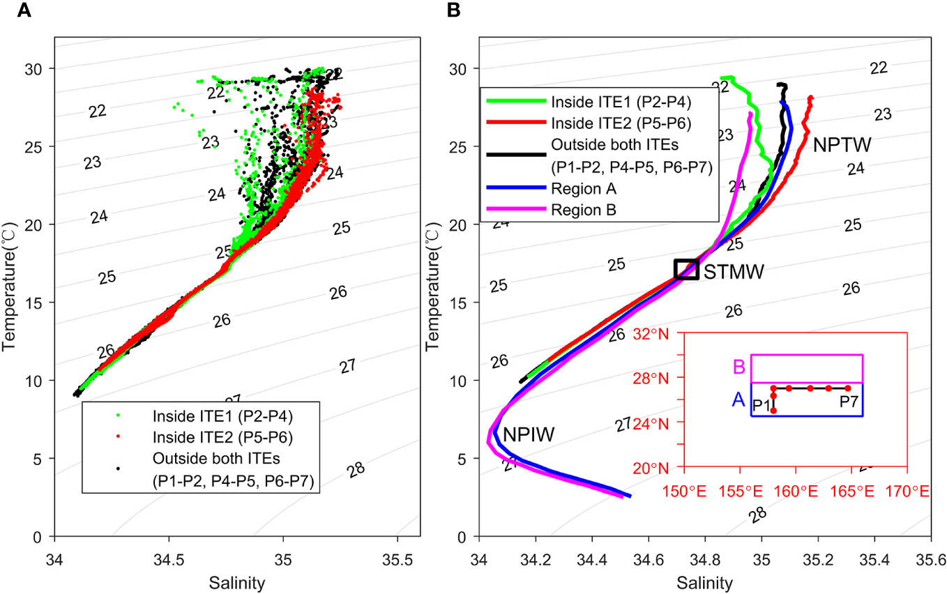
Figure 3 (A) T-S diagram based on glider observations and (B) mean T-S curves based on glider observations and WOA18 monthly climatological data. The green, red and black dots denote the water properties inside ITE1 (P2-P4), inside ITE2 (P5-P6) and outside both ITEs (P1-P2, P4-P5, P6-P7), respectively. The green, red and black lines represent the mean T-S curves inside ITE1 (P2-P4), inside ITE2 (P5-P6) and outside both ITEs (P1-P2, P4-P5, P6-P7), respectively. The blue and magenta lines represent the climatological mean T-S curves during August-October in region A (blue box in the inset) and region B (magenta box in the inset) derived from WOA18 monthly climatological data. The black box in (B) shows the T and S ranges of the STMW.

Before describing the thermohaline properties inside the observed ITEs, it is necessary to briefly introduce the main water masses in the northwestern subtropical Pacific Ocean. As shown in Figure 3B, the T-S curves show a reversed “S” shape, with two vertical salinity extrema featuring two important water masses: the subsurface high-salinity (S > 34.8) North Pacific Tropical Water (NPTW) between 22.5-25.5σ_θ and the low-salinity (S< 34.3) North Pacific Intermediate Water (NPIW) between 26.6-27.1σ_θ (Talley, 1993; Suga et al., 2000). Beneath the NPTW, the low PV STMW exits within the main thermocline (Hanawa, 1987), which splits the main thermocline into upper and lower portions. Following Xu et al. (2017), we define the STMW thickness as a continuous layer between 25.0-25.4σ_θ with PV< 2×10^-10m^-1s^-1, and the T and S ranges of the STMW are between 16.54-17.67°C and 34.69-34.77 (shown as black box in Figure 3B) from our calculation using the glider data and the WOA18 climatological data.

As shown in Figure 3A, the water properties inside ITE1 (green dots) were similar to those in ambient waters (black dots), while the water properties inside ITE2 (red dots) exhibited a relatively isolated feature compared to those in ambient waters (black dots) and inside ITE1 (green dots).

The mean T-S curves in the study area are shown in Figure 3B. The blue and magenta lines can be treated as the basic state of the water properties in the glider observation region (region A) and its northern adjacent area (region B). The water properties outside both ITEs observed by the glider (the black line) were very close to the basic state of region A (the blue line), and the water inside ITE1 (the green line) seemed to be a mixture of region A (the blue line)and region B (the magenta line) water, which indicates that ITE1 may have been locally formed in region A or region B. On the other hand, the water properties inside ITE2 (the red line) were different from the basic state of both region A (the blue line) and region B (the magenta line), which suggests that there may be a remote origin for ITE2.

3.3 Validation of CMEMS reanalysis

In order to investigate the structure, evolution and dynamics of ITE1 and ITE2, we employ the CMEMS reanalysis product. Previous studies have shown that observed ITEs can be well reproduced by CMEMS reanalysis (Lin et al., 2017; Ding et al., 2022).

As shown in Figure 4, the main patterns of T, S, σ_θ and PV distributions along transect P are qualitatively similar to the glider observations, and most observed features in Figure 2 are effectively reproduced by the CMEMS reanalysis. ITE1 and ITE2 can be clearly detected in Figure 4. The positions of these two ITEs are accurately reproduced and the lens-shaped structures can be seen in isopleth distributions between P2-P4 and P5-P6, although the isohalines do not form a complete dome-shaped structure above 200 m between P2-P4. The lowest PV is also located at 25.0-25.4σ_θ between P2-P4 and P5-P6, and the 25.0-25.4σ_θ averaged PV shows similar variation along transect P compared to the glider observations (Figures 4C, D). Furthermore, the observed low-salinity water located at 0-50 m between P3-P4 (Figure 2B) is also seen in Figure 4B, which enables us to further investigate the dynamics of ITE1 using CMEMS reanalysis.

Figure 4

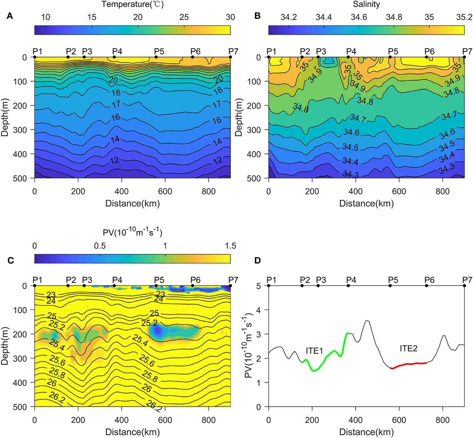
Figure 4 Vertical distributions of (A) temperature (°C), (B) salinity, (C) potential density (kg/m³, contours), PV (10^-10m^-1s^-1, shading) and (D) 25.0-25.4σθ averaged PV variation along transect P based on the CMEMS reanalysis during the glider observation period. In (D), the PV variation within ITE1 (ITE2) is colored in green (red).

The above comparisons suggest that the CMEMS reanalysis is able to reproduce the basic features of ITE1 and ITE2.

It is worth noting that our calculation shows the absolute vorticity was largely dominated by the planetary vorticity (f) in the ITEs based on the CMEMS reanalysis (figure not shown), in consistence with the results in Xu et al. (2017). Thus the relative vorticity (ζ) was ignored in the PV calculation in this study.

3.4 Evolutionary characteristics of ITE1

As noted above, there was a patch of low-salinity water at 0-50 m between P3-P4 (Figures 2B, 4B). Using the CMEMS reanalysis, we will examine the evolution of the fresh water, the ITE1 structure and the connection between them.

Figure 5A shows the 5-day evolution of 0-50 m averaged S distributions near transect P during August-September 2019. During 16-25 August, the fresh water was located to the north of transect P and the 0-50 m averaged S was relatively high between P2-P4. During 26 August - 14 September, the fresh water extended southwestward and gradually occupied the area between P2-P4. After 15 September, the fresh water moved westward gradually and the 0-50 m averaged S between P2-P4 increased again.

Figure 5

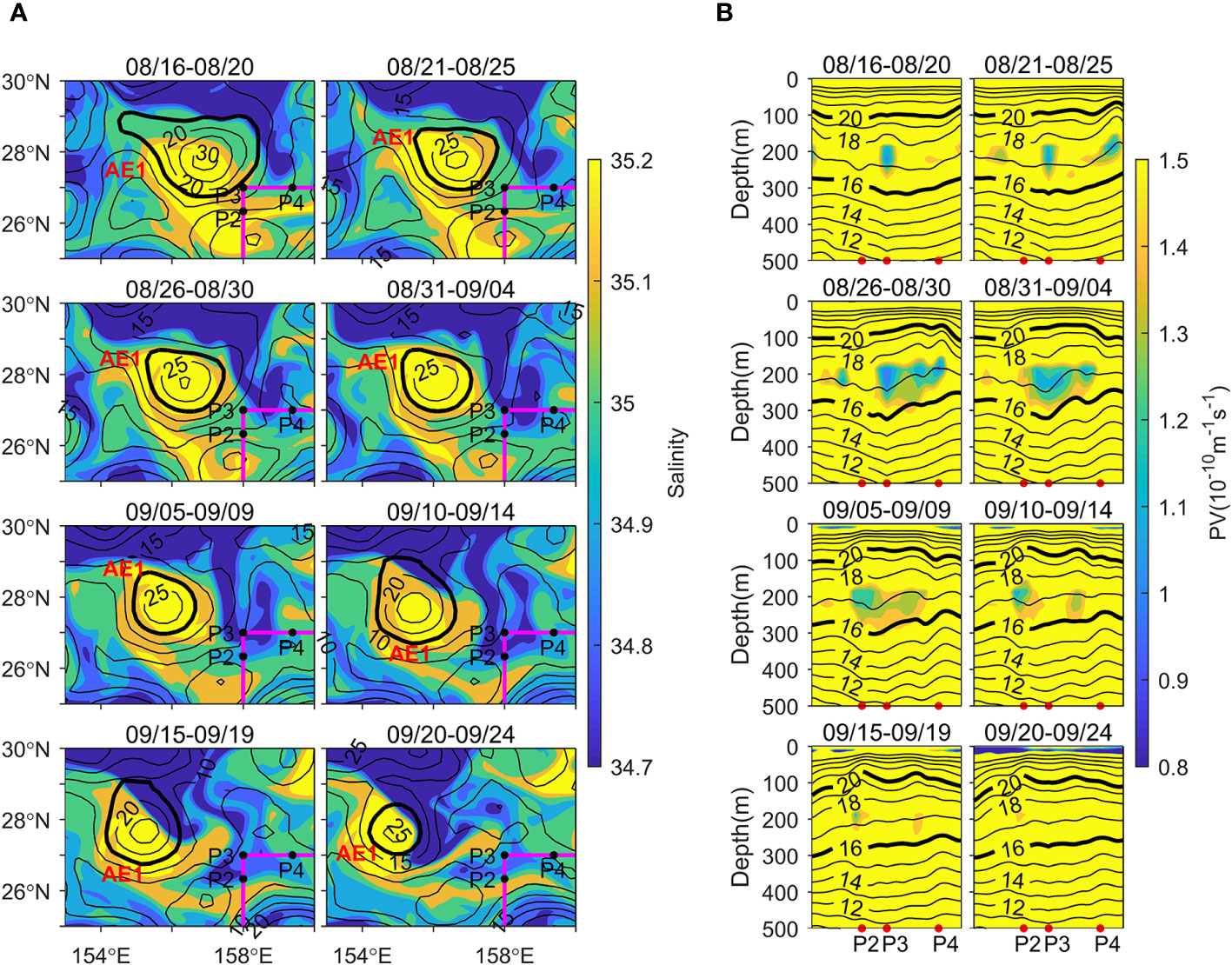
Figure 5 5-day averaged (A) spatial distributions of SLA (cm, contours) and 0-50 m averaged salinity (shading) near transect P and (B) vertical distributions of temperature (°C, contours) and PV (10^-10m^-1s^-1, shading) along transect P during August-September 2019 based on the CMEMS reanalysis. The magenta line represents transect P and P2-P4 are marked. Thick black contours in (A) represent the outermost closed SLA contour associated with AE1.

Figure 5B shows the corresponding 5-day evolution of T and PV distributions along transect P. There was an obvious increase in low PV water volume and a lens-shaped structure developed between P2-P4 when the fresh water arrived at transect P during 26 August - 14 September. In contrast, before the fresh water arrived (during 16-25 August) and after it gradually moved away from transect P (after 15 September), there was no obvious lens-shaped structure and the volume of low PV water was much smaller between P2-P4.

Figure 5A also shows the 5-day evolution of SLA near transect P. During August-September 2019, there was an anticyclonic eddy (AE1) near transect P, which had higher salinity at 0-50 m than the surrounding waters. However, AE1 was not associated with ITE1 since it kept moving westward and was already located to the west of transect P before ITE1 formed (before 26 August).

The variation of 5-day averaged T-S curves of the area near P3 (Figure 6) shows the evolution of ITE1 more clearly. The green line can be treated as the basic state of the water properties of the area near P3. Before ITE1 formed (1-25 August), the T-S curves (the red curves) deviated from the basic state to the right because the AE1 with high salinity in the upper layer was located nearby. During the occurrence of ITE1 (26 August - 14 September), while the fresh water gradually occupied the area between P2-P4, the T-S curves (the blue curves) started to deviate from the basic state to the left. After ITE1 decayed (15 September -29 October), the T-S curves (the black curves) returned to the basic state gradually, and the water properties of the area near P3 became very close to its basic state after 24 September.

Figure 6

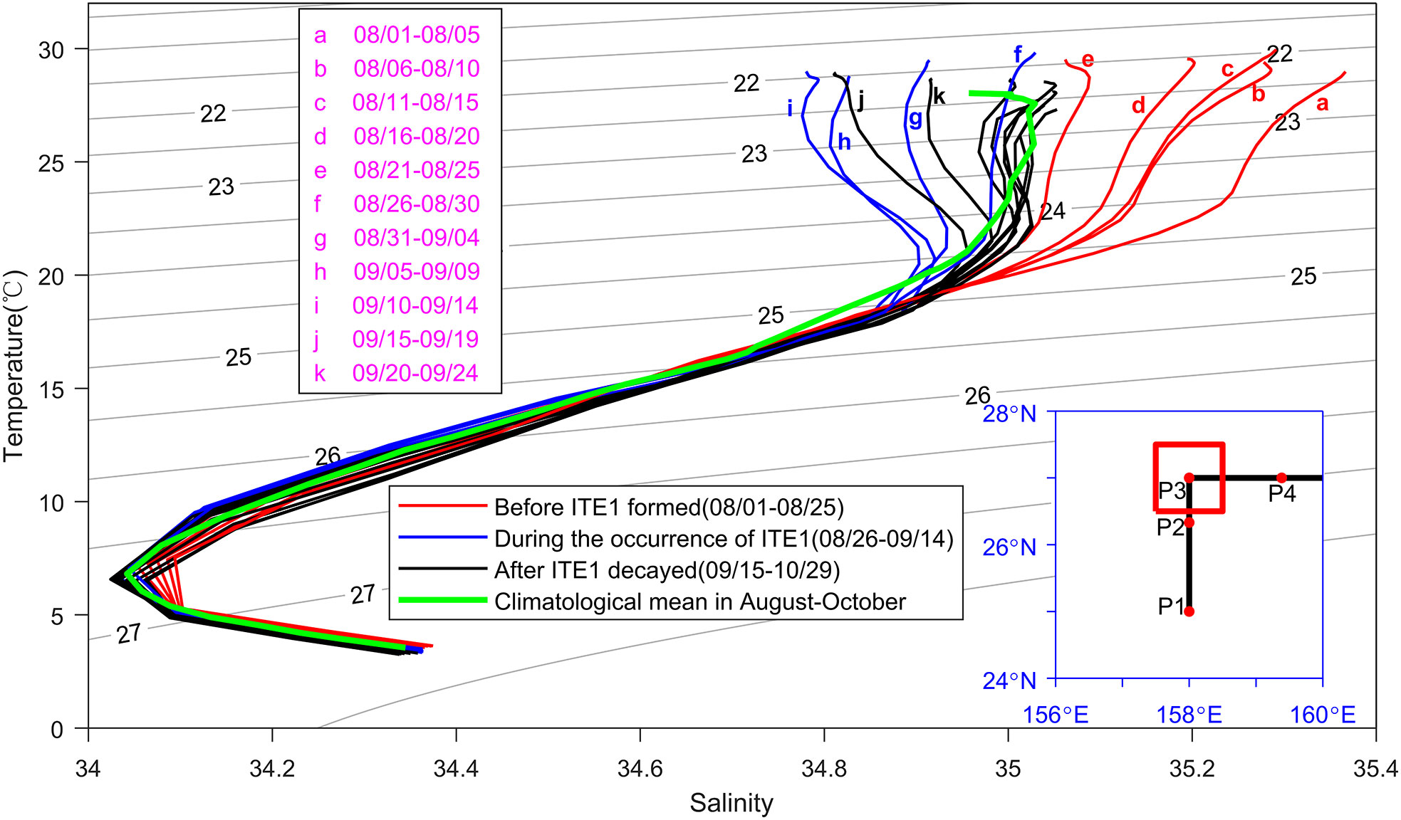
Figure 6 Variation of 5-day averaged T-S curves of the area near P3 (red box in the inset) during August-October 2019 based on the CMEMS reanalysis. The red, blue and black lines represent the T-S curves averaged in the red box before ITE1 formed (1-25 August), during the occurrence of ITE1 (26 August - 14 September) and after ITE1 decayed (15 September - 29 October), respectively. The green line represents the climatological mean T-S curve during August-October averaged in the red box derived from WOA18 monthly climatological data.

According to the above results, we infer that the formation and evolution of ITE1 were highly associated with the existence and movement of the fresh water at 0-50 m between P2-P4. Possible generation mechanism of ITE1 will be further discussed in Section 4.

3.5 Vertical structure of ITE2 based on the CMEMS reanalysis

Figure 7A shows the spatial map of SLA in the study area on 26 September 2019. As shown in the figure, ITE2 was clearly exhibited in the map of SLA. The glider crossed the southern part of an anticyclonic eddy (AE2) between P5-P6 during mid-September - early October 2019. Figure 7A also shows the track of AE2 derived from the META2.0 DT dataset. AE2 originated at S (167.82°E, 30.05°N) on 11 April 2019, then moved southwestward and finally disappeared at E (154.71°E, 27.70°N) on 22 February 2020.

Figure 7

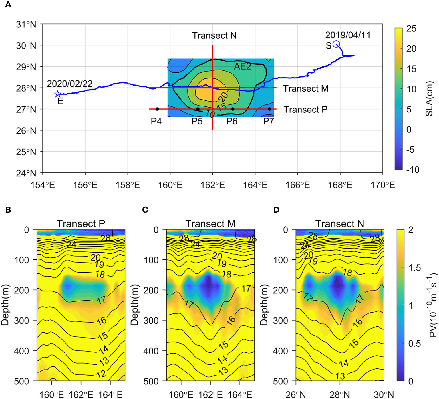
Figure 7 (A) Spatial map of SLA (cm, shading contours) in the northwestern subtropical Pacific Ocean on 26 September 2019. The thick black contour represents the outermost closed SLA contour associated with AE2. The blue line is the track of AE2 derived from the META2.0 DT dataset, S (blue open circle) and E (blue open star) indicate the generation and dissipation locations of AE2. Transect P (the glider track) is the zonal transect crossing the southern part of AE2. Transect M (N) is the zonal (meridional) transect crossing AE2 center. P4-P7 are marked as black dots. (B–D) Vertical distributions of temperature (°C, contours) and PV (10^-10m^-1s^-1, shading) along transect P, M and N on 26 September 2019 based on the CMEMS reanalysis.

Just as we guessed, the glider actually crossed ITE2 without entering its core. Figures 7B–D show the vertical distribution of T along transect P, M and N on 26 September 2019 based on the CMEMS reanalysis. The lens-shaped structure was not that clear at transect P (the glider track), similar to Figure 2A. In contrast, the lens-shaped structure was very clear at both the zonal and meridional transects crossing the AE2 center (transect M and N). The above results demonstrate that the lens-shaped structure of ITE2 was also very clear near its core and ITE2 displayed clear signals at the surface as AE2.

To examine the vertical structure of ITE2 during its whole lifespan, we show the vertical distributions of T and its anomaly (T´), S and its anomaly (S´) and PV of composite ITE2 along the zonal and meridional transects crossing AE2 center during the AE2 lifespan (11 April 2019 - 22 February 2020) based on the CMEMS reanalysis (Figure 8). Here the T, S and PV structures of composite ITE2 mean the T, S and PV distributions along the zonal and meridional transects averaged from 11 April 2019 to 22 February 2020. Different points with positive or negative value of Δx (Δy) at the zonal (meridional) transect indicate that they are located east or west (north or south) of the AE2 center, respectively. The T´ (S´) was calculated as the difference from the mean T (S) value at the same depth. The upper isotherms and isohalines (T≥18°C, S≥34.8) bend upward above 200 m, while the lower ones (T ≤ 17°C, S ≤ 34.7) bend downward at 200-1000 m. A clear lens-shaped structure can be seen, although the “dome” of the lens above 200 m is much less prominent compared to the “base” below 200 m (Figures 8A, B, D, E).

Figure 8

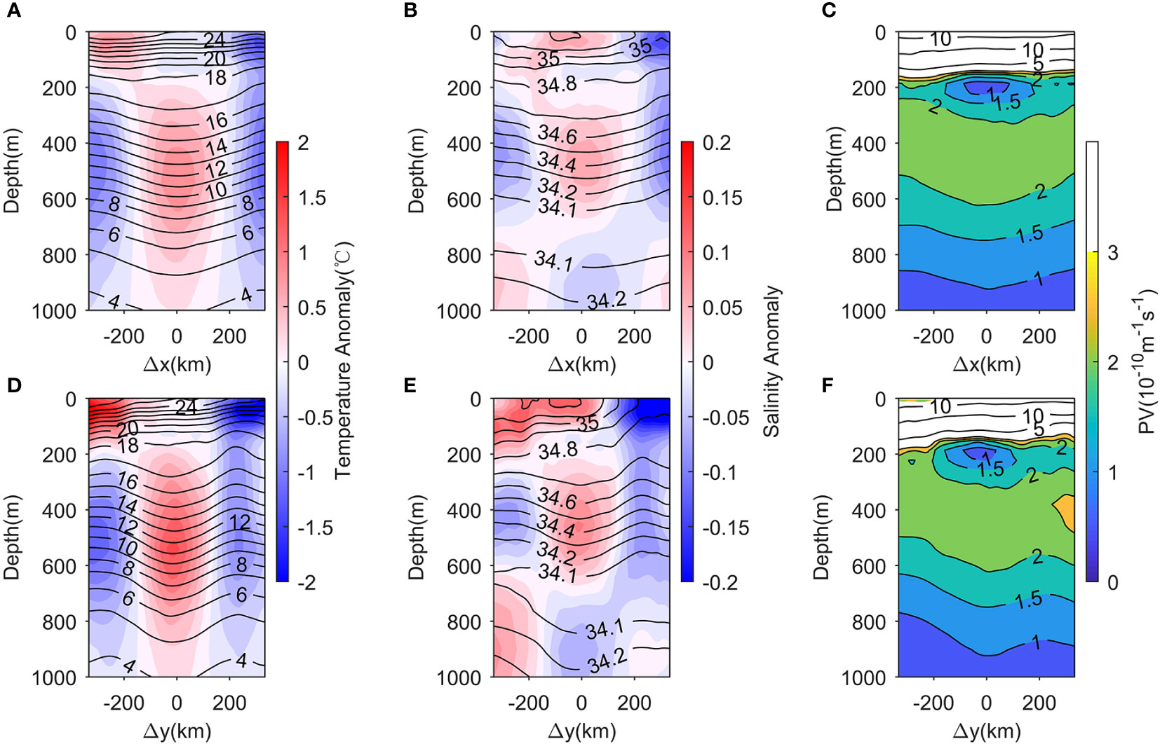
Figure 8 Vertical distributions of (A, D) temperature (°C, contours) and its anomaly (°C, shading), (B, E) salinity (contours) and its anomaly (shading) and (C, F) PV (10^-10m^-1s^-1) of composite ITE2 along the zonal (top row) and meridional (bottom row) transects crossing AE2 center during the AE2 lifespan (11 April 2019 - 22 February 2020) based on the CMEMS reanalysis.

The water at 200-1000 m within ITE2 is warmer than the surrounding waters, with T´ magnitude >0.8°C located at ~400-620 m (~300-720 m) in zonal (meridional) direction (Figures 8A, D). The meridional T´ even exceeds 1.4°C at ~540 m (Figure 8D). Due to the slight upward bending of isotherms, only weak negative T´ (> -0.2°C) exists within ITE2 above 200 m (Figures 8A, D).

Due to the existence of NPTW and NPIW, the S´ displayed an obviously different pattern (Figures 8B, E). The water at 200-700 m (700-1000 m) within ITE2 is saltier (fresher) than the surrounding waters. Strong positive S´ (> 0.06) is located at ~400-540 m (~300-600 m) in zonal (meridional) direction. The meridional positive S´ exceeds 0.1 at ~450 m (Figure 8E). The S´ is negative at 700-1000 m within ITE2 and large zonal (meridional) negative S´ with magnitude< -0.02 (-0.04) is located at 800-1000 m. Similar to the T´ pattern, the S´ fields show relatively weak negative values (> -0.02) within ITE2 at 100-200 m. As indicated in Figures 8C, F, the STMW (PV< 2×10^-10m^-1s^-1) is trapped inside ITE2 and the lowest PV (< 1.5×10^-10m^-1s^-1) is located at ~170-250 m inside the ITE2 core.

The above results demonstrate that the T´ and S´ induced by ITE2 can reach 1000 m or even deeper, and the meridional T´ and S´ are slightly stronger than the zonal ones below 200 m.

3.6 Vertical structure of ITE2 from Argo observations

According to the tracks of Argo2903424, Argo2903427 and AE2 (Figures 7A, 9A, E), we found that Argo2903424 (Argo2903427) was captured by AE2/ITE2 during 20 June - 22 July 2019 (10 December 2019 - 8 January 2020). Figure 9 shows the time-depth plots of T, T´, S, S´, σ_θ and PV for Argo2903424 and Argo2903427. The T´ (S´) was calculated as the difference between the observed T (S) value of each profile and the mean T (S) value of all the profiles used. The lens-shaped structure, with isopleths bending upward (downward) above (below) 200 m and lower PV located at 25.2-25.4σ_θ, was observed when the two Argo floats were trapped inside AE2/ITE2. The water in the eddy core below 200 m was warmer than the surrounding waters, and the T´ within 300-800 m exceeded 0.5°C and reached 1.35°C (1.00°C) at ~440 m (400 m) based on Argo2903424 (Argo2903427) observations (Figures 9B, F).

Figure 9

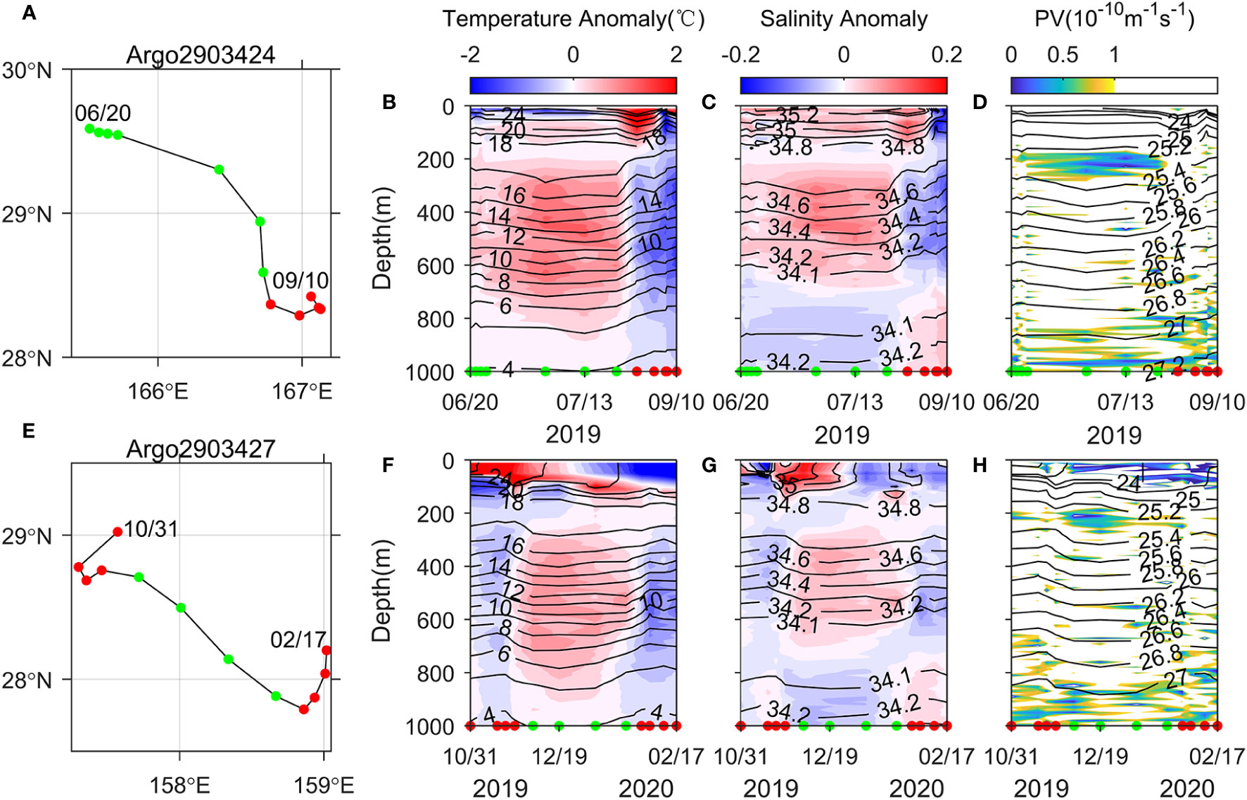
Figure 9 (A, E) Argo tracks and time-depth plots of (B, F) temperature (°C, contours) and its anomaly (°C, shading), (C, G) salinity (contours) and its anomaly (shading), (D, H) potential density (kg/m³, contours) and PV (10^-10m^-1s^-1, shading) for Argo2903424 (top row) and Argo2903427 (bottom row). The green (red) solid circles represent Argo profiles inside (outside) AE2.

Similar to Figures 8B, E, The water in the eddy core within 200-700 m (below 700 m) was saltier (fresher) than the surrounding waters, with S´ reaching 0.12 (0.08) and -0.04 (-0.05) at~450 m (520 m) and ~930 m (940 m) based on Argo2903424 (Argo2903427) observations (Figures 9C, G). Notably, the upward bending of isopleths was much less prominent, and the T’ and S’ within AE2/ITE2 were relatively weak above 200 m (Figures 9B, C, F, G).

3.7 Thermohaline properties inside ITE2

As shown in Figure 10A, in the upper layer (above 25.0 σ_θ), the water properties inside ITE2 derived from the glider (the red line), Argo2903424 (the cyan dots), Argo2903427 (the magenta dots) and the daily CMEMS reanalysis data (the grey dots) were generally similar but different from those inside ITE1 (the green line) and the basic state of region A (the blue line) where ITE2 was detected by the glider. While moving southwestward, the water inside ITE2 still kept saltier than those inside ITE1 and in region A.

Figure 10

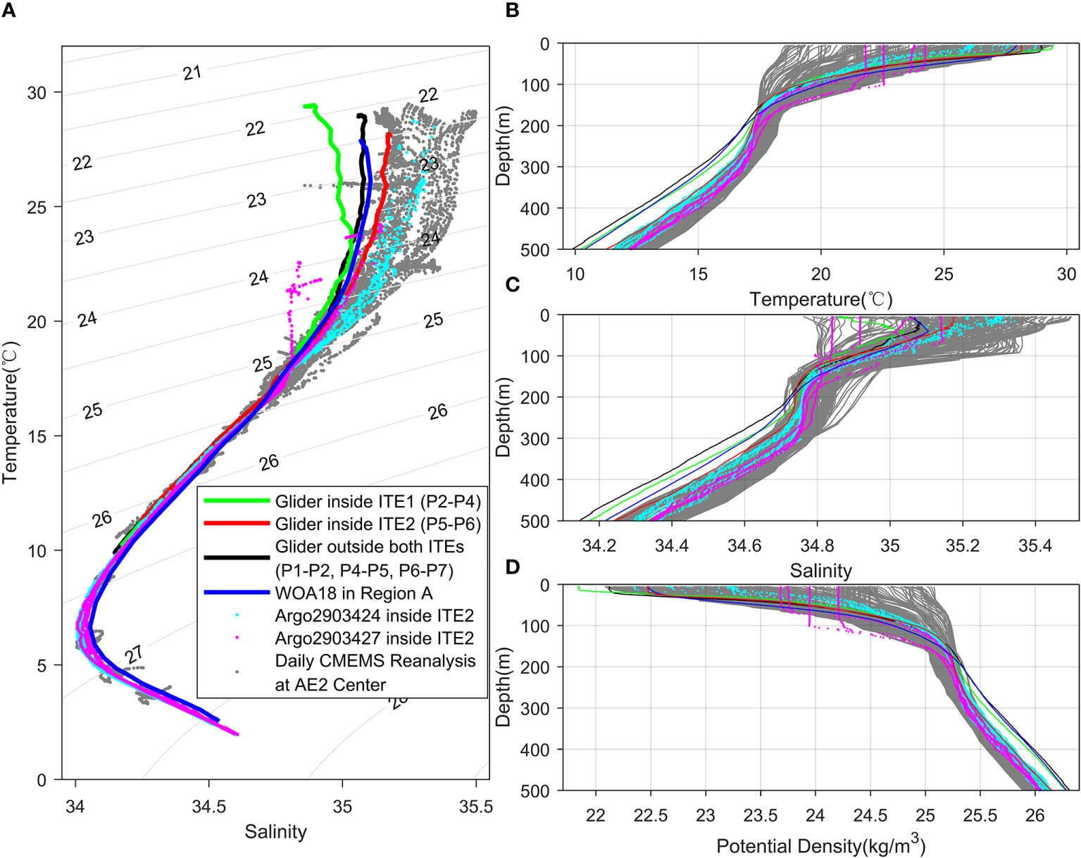
Figure 10 (A) T-S diagram and vertical profiles of (B) temperature (°C), (C) salinity and (D) potential density (kg/m³). The green, red and black lines represent the mean thermohaline properties inside ITE1 (P2-P4), inside ITE2 (P5-P6) and outside both ITEs (P1-P2, P4-P5, P6-P7) based on glider observations. The blue line represents the climatological mean thermohaline properties during August-October in Region A (shown as blue box in Figure 3B) derived from WOA18 monthly climatological data. The cyan and magenta dots denote the thermohaline properties inside ITE2 observed by Argo2903424 and Argo2903427 (the locations of the Argo profiles used are shown as green solid circles in Figures 9A, E). The gray dots and gray lines represent the daily thermohaline properties at AE2 center during the AE2 lifespan (11 April 2019 - 22 February 2020) based on the CMEMS reanalysis data.

As shown in Figures 10B–D, while moving southwestward, the water properties inside ITE2 above 170m varied dramatically. The T, S and σ_θ at the surface varied between 18.54-29.48 °C, 34.76-35.50 and 22.08-25.07 kg/m³ respectively during the AE2 lifespan (11 April 2019 - 22 February 2020) based on the daily CMEMS reanalysis data. It is worth noting that, as the season changed, a much deeper mixed layer was found in the magenta dots (observed by Argo2903427 during 10 December 2019 - 8 January 2020) compared to those in the red line (observed by the glider during 18 September - 3 October 2019) and the cyan dots (observed by Argo2903424 during 20 June - 22 July 2019). Below 170m, the water properties inside ITE2 (the red line, cyan dots, magenta dots and grey lines) became close and distinguished from the colder, fresher and denser water inside ITE1 (the green line) and in region A (the blue line).

The above results further confirm that ITE2 may have a remote origin compared to ITE1.

4 Discussion

The typical feature of anticyclonic ITEs is the lens-shaped structure in isopleth distributions, and the existence of low PV water inside anticyclonic ITEs is thought to be the major reason for this structure. In this section, we will investigate possible generation mechanisms for ITE1 and ITE2 by identifying the source of the low PV water based on the CMEMS reanalysis. In addition, the energy source for ITE1 is also examined by eddy energetics analysis.

4.1 Possible generation mechanism of ITE1

Considering that P3 was probably located within the core of ITE1 during 26 August - 14 September 2019, we show the time-depth plots of T, S, stratification (N²) and PV at P3 during August-September 2019 based on the CMEMS reanalysis to investigate the possible generation mechanism of ITE1 (Figure 11). The stratification, or squared buoyancy frequency, was calculated as:

Figure 11

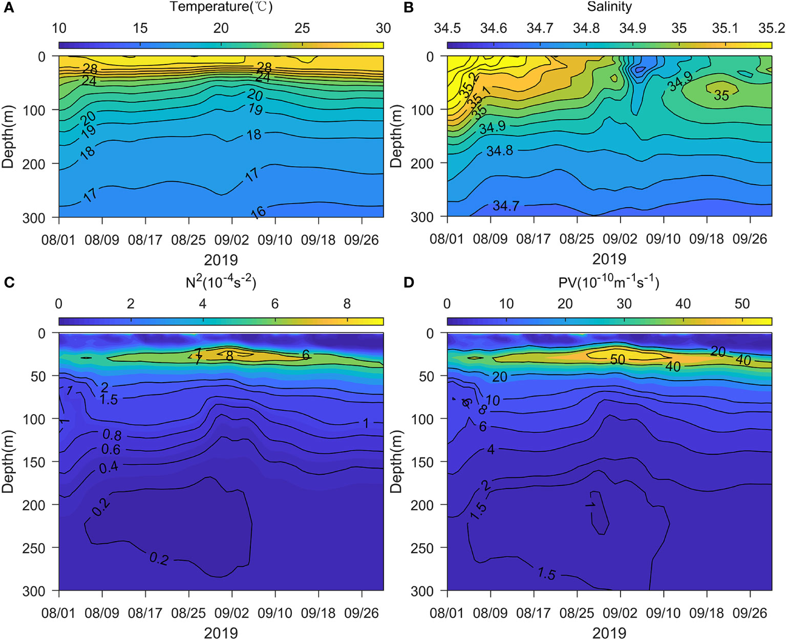
Figure 11 Time-depth plots of (A) temperature (°C), (B) salinity, (C) squared buoyancy frequency (10^-4s^-2) and (D) PV (10^-10m^-1s^-1) at P3 during August-September 2019 based on the CMEMS reanalysis.

$${\text{N}}^2=-\frac{\text{g }}{{\text{σ}}_{\text{θ}}}\frac{\partial {\text{σ}}_{\text{θ}}}{\partial \text{z}},$$

where g is the gravity acceleration, σ_θ is potential density and $\frac{\partial {\text{σ}}_{\text{θ}}}{\partial \text{z}}$ is the vertical gradient of potential density.

ITE1 with a lens-shaped structure can be seen below 50 m (120 m) in the T (S) distribution during 26 August - 14 September while a patch of fresh water was present at P3 above 50 m (Figures 11A, B). It is worth noting that the isotherms and isohalines bounding the lens-shaped structure did not outcrop, which indicates that the low PV water within ITE1 could not originate from the surface through ventilation process.

Previous studies have demonstrated that the formation of lens-shaped structures in the subsurface may be related to local salinity decreases in the surface or near surface layer (Lin et al., 2017; He et al., 2020). Lin et al. (2017) reported a mesoscale lens-shaped structure in the southwestern South China Sea from cruise measurements conducted of the coast of Vietnam in September 2007 and proposed that the water within the lens stemmed largely from the local mixed-layer water which was capped by the Mekong River plume. He et al. (2020) suggested that decreased sea surface salinity may result in changes in upper ocean stratification and the formation of anticyclonic cold-core eddies in the Bay of Bengal.

Similarly, we infer that ITE1 was generated due to the stratification change induced by the near surface salinity decrease. Since the PV is essentially determined by stratification, it showed nearly the same variation as the stratification at P3 (Figures 11C, D). During 26 August - 14 September while the fresh water was present at P3 above 50 m, both the stratification and PV at 15-40 m were significantly enhanced. In contrast, the stratification and PV at 75-170 m were obviously reduced at the same time. According to the above analysis, we conclude that the local salinity-forced restratification (He et al., 2020) due to the arrival of fresh water above 50 m caused a PV decrease in the subsurface and finally resulted in the generation of ITE1. The PV between 75-170 m at P3 reached its minimum on 2 September, which is consistent with the glider observations (green line in Figure 2D).

4.2 Energy source for ITE1

Previous studies have indicated that the baroclinic and barotropic instabilities are responsible for subsurface-intensified eddies generation east of the Philippines (Xu et al., 2020) and are also considered as the major energy sources for mesoscale eddies in the KE region (Waterman et al., 2011; Yang and Liang, 2016). Focusing on these two instabilities, we perform the eddy energetics analysis to further investigate the energy source for ITE1.

Following Tsujino et al. (2006), the barotropic (BT) conversion rate from the mean kinetic energy (MKE) to eddy kinetic energy (EKE), which indicates the barotropic instability, is defined as:

$${\text{R}}_{\text{BT}}=-{\text{ρ}}_0[{\text{u}}^{\prime }{\text{u}}^{\prime }\frac{\partial \overline{\text{u}}}{\partial \text{x}}+{\text{u}}^{\prime }{\text{v}}^{\prime }(\frac{\partial \overline{\text{u}}}{\partial \text{y}}+\frac{\partial \overline{\text{v}}}{\partial \text{x}})+{\text{v}}^{\prime }{\text{v}}^{\prime }\frac{\partial \overline{\text{v}}}{\partial \text{y}}],$$

Where ${\rho }_0$ is the reference density of 1025 kg/m³, $\overline{u}(\overline{v})$ is the zonal (meridional) velocity in the mean field, and $u^{\prime }(v^{\prime })$ is the zonal (meridional) perturbed velocity in the eddy field. The baroclinic (BC) conversion rate from mean potential energy (MPE) to eddy potential energy (EPE), which is associated with the baroclinic instability, is defined as:

$${\text{R}}_{\text{BC}}=-\frac{{\text{g}}^2}{{\text{ρ}}_0\overline{{\text{N}}^2}}({\text{u}}^{\prime }{\text{ρ}}^{\prime }\frac{\partial \overline{\text{ρ}}}{\partial \text{x}}+{\text{v}}^{\prime }{\text{ρ}}^{\prime }\frac{\partial \overline{\text{ρ}}}{\partial \text{y}}),$$

where g is the gravity acceleration, N² is the squared buoyancy frequency, and $\overline{\rho }({\rho }^{\prime })$ is the density in the mean (eddy) field. Note that the mean and eddy fields in our eddy energetics analysis are defined as a long-time (61 days in our case) averaged field and the deviation from it.

We show the spatial distributions of SLA and the BT and BC conversion rates at 92 m before (1-25 August 2019; Figures 12A, D), during (26 August-14 September 2019; Figures 12B, E) and after (15-30 September 2019; Figures 12C, F) the occurrence of ITE1. The mean fields of u, v, ρ and N² in Figure 12 were calculated as the mean values during 1 August - 30 September 2019. Different from ITE2, ITE1 displayed no signals at the surface. The AE1 was not associated with ITE1 since it was already located to the west of transect P before ITE1 was generated (Figures 12B, E). A positive BT (BC) conversion rate indicates the transfer of energy from the mean field to the eddy field, which is favorable for subsurface eddies generation (Xu et al., 2020). During the occurrence of ITE1, larger positive BC can be seen in the area where ITE1 was observed (the green box area) than in the surrounding area (Figure 12E), which indicates the baroclinic instability may be the energy source for ITE1. In contrast, the BC in the green box area became smaller after ITE1 decayed (Figure 12F). It is worth noting that the strong positive BC in the green box area before the occurrence of ITE1 (Figure 12D) was probably due to the strong baroclinic instability at the southern edge of AE1. On the other hand, there was no obvious positive BT in the green box area during August-September 2019 (Figures 12A–C), which indicates the barotropic instability was not responsible for ITE1 generation.

Figure 12

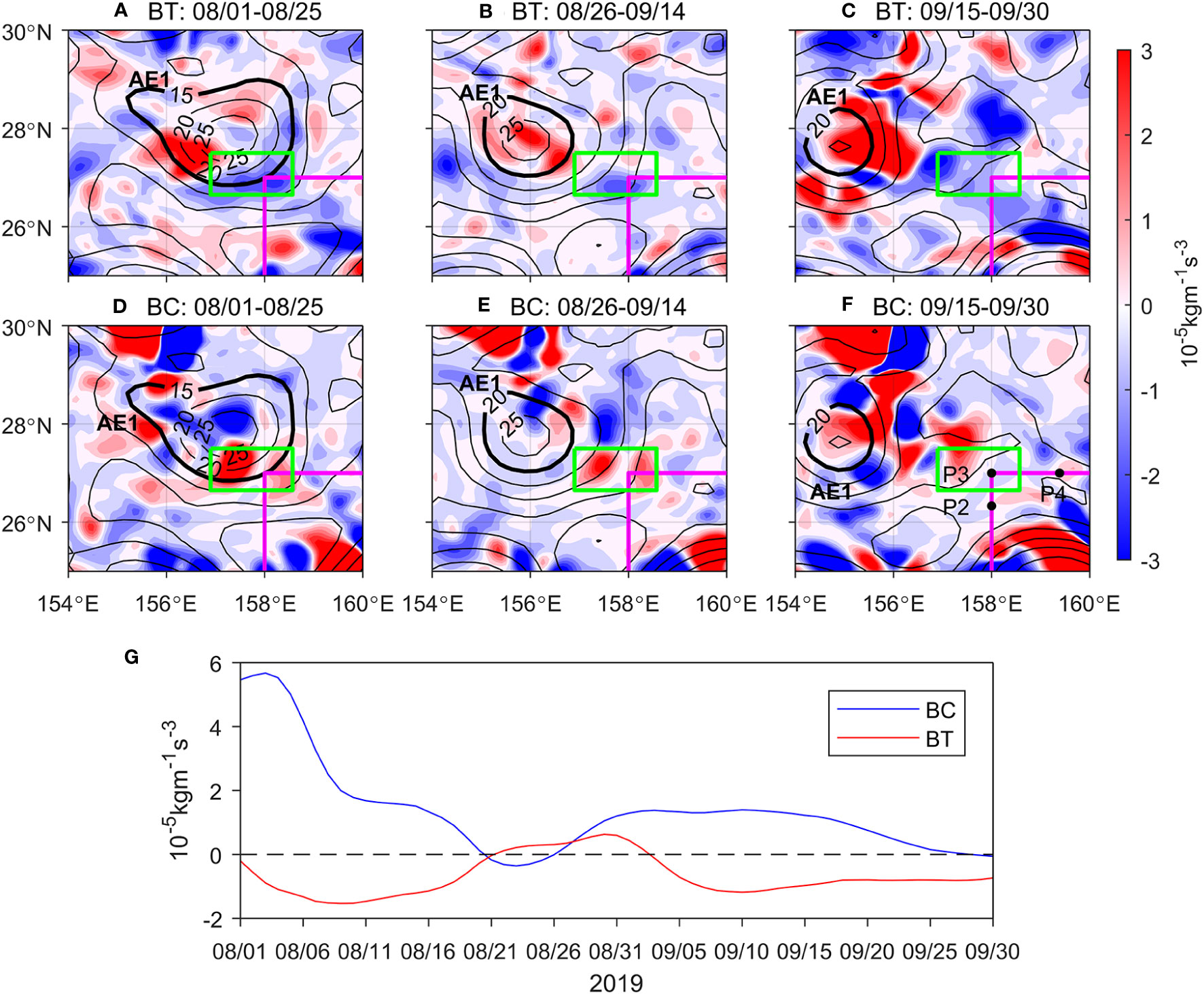
Figure 12 Spatial distributions of SLA (cm, contours) and energy conversion rates (10^-5kgm^-1s^-3, shading) at 92 m during (A, D) 1-25 August, (B, E) 26 August-14 September and (C, F) 15-30 September 2019 based on the CMEMS reanalysis. (G) Time series of energy conversion rates (10^-5kgm^-1s^-3) at 92 m averaged in the green box during August-September 2019. The magenta line represents transect P and P2-P4 are marked as black dots. Thick black contours represent the outermost closed SLA contour associated with AE1.

The daily evolution of BT and BC conversion rates averaged in the green box area at 92m are also shown in Figure 12G. The BC decreased sharply from approximately 5.6×10^-5kgm^-1s^-3 to near 0 during 1-25 August as AE1 gradually moved westward. The BC started to increase during the occurrence of ITE1 (26 August-14 September) and then decreased again after ITE1 decayed (15-30 September). In contrast, positive BT only appeared on 21 August - 2 September.

Figure 13 shows the time-depth plots of BT and BC conversion rates averaged in the green box (shown in Figure 12) during August-September 2019. Positive BT was found between 200-600m during 1-3 August and above 800m during 21 August-2 September. Due to the influence of AE1, extremely strong positive BC appeared above 400 m before 20 August with its maximum value exceeding 4×10^-5kgm^-1s^-3. In addition, another area of strong positive BC was located between 50-170 m during the occurrence of ITE1 (26 August-14 September) with its maximum value exceeding 1×10^-5kgm^-1s^-3.

Figure 13

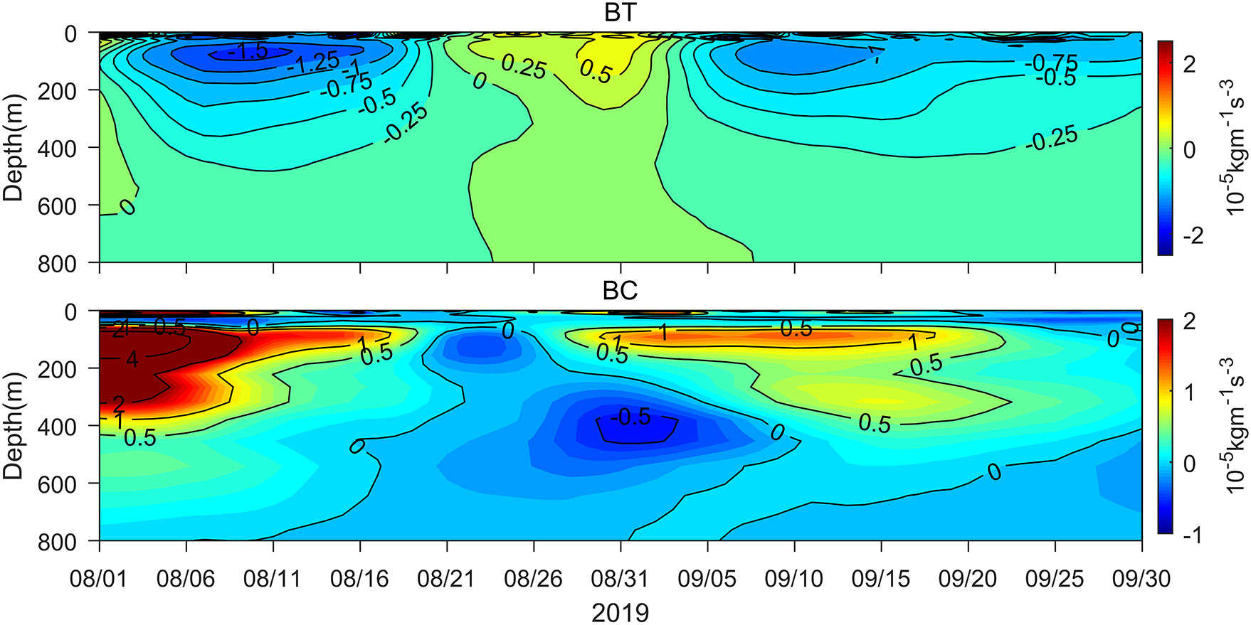
Figure 13 Time-depth plots of energy conversion rates (10^-5kgm^-1s^-3) averaged in the green box (shown in Figure 12) during August-September 2019 based on the CMEMS reanalysis.

According to the above results, we conclude that the baroclinic instability at 50-170 m might have played a major role in ITE1 generation.

4.3 Possible generation mechanism of ITE2

AE2/ITE2 was generated at S (167.82°E, 30.05°N) on 11 April 2019, which is also within the main formation region of STMW. We thus examine the evolution of σ_θ, PV and SLA at S to explore the possible generation mechanism for ITE2 (Figure 14).

Figure 14

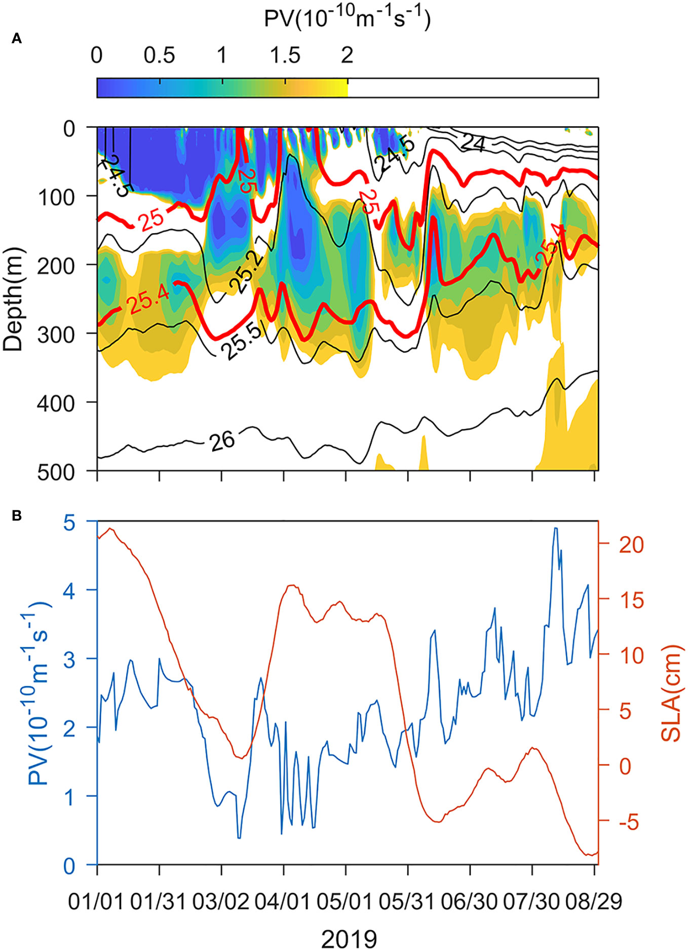
Figure 14 (A) Time-depth plots of potential density (kg/m³, contours) and PV (10^-10m^-1s^-1, shading) and (B) time series of 25.0-25.4σ_θ averaged PV (10^-10m^-1s^-1) and SLA (cm) at S (shown as blue open circle in Figure 7A) during January-August 2019. The 25.0 and 25.4 σ_θ isopycnals are thickened and colored in red to highlight the STMW.

The STMW, which is defined as the water between 25.0-25.4σ_θ with PV<2×10^-10m^-1s^-1 (Xu et al., 2017), was present at S in January-August 2019 and ventilated during 10-12 March and 30 March-17 April (Figure 14A), resulting in reduced PV in the STMW density layer (25.0-25.4σ_θ) at S (Figure 14B). During the second ventilation process (30 March - 17 April 2019), while the upper boundary of the STMW (25.0σ_θ) outcropped for 19 continuous days, the SLA at S underwent a rising process (Figure 14B) and AE2 was finally generated there. As a result, the newly formed STMW with lower PV was trapped in AE2 and a lens-shaped structure developed in the subsurface. Subduction of the STMW caused the generation of ITE2. The low PV water within the lens originated from the STMW formation zone.

5 Conclusion

Two anticyclonic ITEs (ITE1 and ITE2) were detected by an underwater glider in the northwestern subtropical Pacific Ocean during August-October 2019. ITE1 was observed between P2 (158°E, 26.33°N) - P4 (159.38°E, 27°N) during 30 August - 7 September 2019, while ITE2 was observed between P5 (161.31°E, 27°N) - P6 (162.94°E, 27°N) during 18 September - 3 October 2019. They both exhibited a lens-shaped vertical structure within the thermocline with their cores located at ~170 m. The low PV STMW was found within the cores of these two ITEs.

The lens-shaped structure of ITE1 observed by the glider was very clear since the glider seemed to have moved into its core during the observation. Further analysis reveals that ITE1 displayed no signals at the sea surface and lasted for about 20 days (26 August-14 September 2019). ITE1 was locally formed and the water inside it was a mixture of local water and the water in the northern adjacent area. During the occurrence of ITE1 (26 August-14 September 2019), a patch of low-salinity water at 0-50 m from the northern adjacent area extended southwestward and gradually occupied the area between P2-P4. The local water was mixed with this fresh water and there was an obvious increase in low PV water volume and a lens-shaped structure developed between P2-P4. In contrast, before the fresh water arrived (16-25 August 2019) and after it gradually moved away from transect P (15-24 September 2019), there was no obvious lens-shaped structure and the volume of low PV water was much smaller between P2-P4.

The lens-shaped structure of ITE2 observed by the glider was less prominent since the glider did not move into its core. Further analysis reveals that the lens-shaped structure of ITE2 was also very clear near its core and ITE2 displayed clear signals at the surface as an anticyclonic eddy (AE2), which originated within the main formation region of STMW on 11 April 2019, then moved southwestward and finally disappeared on 22 February 2020. The vertical structure of composite ITE2 during its lifespan was further investigated based on the CMEMS reanalysis data. Results show that the T´ and S´ induced by ITE2 can reach 1000 m or even deeper. The water in the eddy core was warmer at 200-1000 m and saltier (fresher) at 200-700 m (700-1000 m) than the surrounding waters. Strong positive T´ (>1°C) and S´ (>0.1) appeared between 400-600 m. The T´ and S´ above 200 m induced by ITE2 were relatively weak compared to those below 200 m.

Based on the CMEMS reanalysis data, we investigated possible generation mechanisms for ITE1 and ITE2. The local salinity-forced restratification due to the arrival of the low-salinity water above 50 m between P2-P4 caused a PV decrease in the subsurface and finally resulted in the generation of ITE1. Furthermore, results from eddy energetics analysis suggest that the baroclinic instability at 50-170 m may be the main energy source for ITE1 generation. On the other hand, AE2/ITE2 was remotely generated within the main formation region of STMW on 11 April 2019 when the STMW also outcropped there. As a result, the newly formed STMW with lower PV was trapped in AE2 and a lens-shaped structure developed in the subsurface. Subduction of the STMW caused the generation of ITE2.

Although there is rich surface eddy activity in the northwestern subtropical Pacific Ocean (Yang et al., 2013), few subsurface eddies were found there (Xu et al., 2019). This study provides us with a precious opportunity to better understand the general characteristics, evolutionary process and generation mechanisms of ITEs in this region. ITEs in the northwestern subtropical Pacific Ocean usually carry STMW and travel a long distance, but their influences on STMW formation, distribution and transport remain unclear. Meanwhile, increasing attention has been paid to the influence of ITEs on marine biogeochemical processes during the past few decades. To investigate these influences in greater depth, more observations and modeling studies are needed.

Data availability statement

The original contributions presented in the study are included in the article/supplementary material. Further inquiries can be directed to the corresponding author.

Author contributions

SC: Writing – original draft. JH: Investigation, Formal analysis, Writing – original draft, Data curation. WW: Investigation, Writing – original draft, Data curation, Formal analysis. CJ: Writing – review & editing, Funding acquisition. JX: Writing – review & editing. KL: Writing – review & editing. FK: Writing – review & editing.

Funding

The author(s) declare financial support was received for the research, authorship, and/or publication of this article. This study is supported by the National Key R&D Program of China (No. 2022YFC2803901) and the Global Change and Air-sea Interaction II (GASI-01-NPAC-STsum).

Conflict of interest

The authors declare that the research was conducted in the absence of any commercial or financial relationships that could be construed as a potential conflict of interest.

Publisher’s note

All claims expressed in this article are solely those of the authors and do not necessarily represent those of their affiliated organizations, or those of the publisher, the editors and the reviewers. Any product that may be evaluated in this article, or claim that may be made by its manufacturer, is not guaranteed or endorsed by the publisher.

References

Assassi C., Morel Y., Vandermeirsch F., Chaigneau A., Pegliasco C., Morrow R., et al. (2016). An index to distinguish surface- and subsurface-intensified vortices from surface observations. J. Phys. Oceanogr. 46, 2529–2552. doi: 10.1175/JPO-D-15-0122.1

CrossRef Full Text | Google Scholar

Chelton D. B., Schlax M. G., Samelson R. M. (2011). Global observations of nonlinear Mesoscale eddies. Prog. Oceanog. 91, 167–216. doi: 10.1016/j.pocean.2011.01.002

CrossRef Full Text | Google Scholar

Combes V., Hormazabal S., Di Lorenzo E. (2015). Interannual variability of the subsurface eddy field in the Southeast Pacific. J. Geophys. Res.: Oceans. 120, 4907–4924. doi: 10.1002/2014JC010265

CrossRef Full Text | Google Scholar

Dilmahamod A. F., Aguiar-Gonzalez B., Penven P., Reason C. J. C., De Ruijter W. P. M., Malan N., et al. (2018). SIDDIES corridor: A major east-west pathway of longlived surface and subsurface eddies crossing the subtropical south Indian Ocean. J. Geophys. Res.: Oceans. 123, 5406–5425. doi: 10.1029/2018JC013828

CrossRef Full Text | Google Scholar

Ding Y., Yu F., Ren Q., Nan F., Wang R., Liu Y., et al. (2022). The physical-biogeochemical responses to a subsurface Anticyclonic eddy in the northwest Pacific. Front. Mar. Sci. 8. doi: 10.3389/fmars.2021.766544

CrossRef Full Text | Google Scholar

Gordon A. L., Giulivi C. F., Lee C. M., Furey H. H., Bower A., Talley L. (2002). Japan/East Sea intrathermocline eddies. J. Phys. Oceanogr. 32, 1960–1974. doi: 10.1175/1520-0485(2002)032<1960:JESIE>2.0.CO;2

CrossRef Full Text | Google Scholar

Gordon A. L., Shroyer E., Murty V. S. N. (2017). An Intrathermocline Eddy and a tropical cyclone in the Bay of Bengal. Sci. Rep. 7, 1–8. doi: 10.1038/srep46218

PubMed Abstract | CrossRef Full Text | Google Scholar

Gula J., Blacic T. M., Todd R. E. (2019). Submesoscale coherent vortices in the Gulf Stream. Geophys. Res. Lett. 46, 2704–2714. doi: 10.1029/2019GL081919

CrossRef Full Text | Google Scholar

Hanawa K. (1987). Interannual variations of the winter-time outcrop area of subtropical mode water in the western North Pacific Ocean. Atmosphere-Ocean 25, 358–374. doi: 10.1080/07055900.1987.9649280

CrossRef Full Text | Google Scholar

Hansen C., Kvaleberg E., Samuelsen A. (2010). Anticyclonic eddies in the Norwegian Sea; their generation, evolution and impact on primary production. Deep-Sea. Res. I. 57, 1079–1091. doi: 10.1016/j.dsr.2010.05.013

CrossRef Full Text | Google Scholar

He Q. Y., Zhan H. G., Cai S. Q. (2020). Anticyclonic eddies enhance the winter barrier layer and surface cooling in the Bay of Bengal. J. Geophys. Res.: Oceans 125, e2020JC016524. doi: 10.10292020/JC016524

CrossRef Full Text | Google Scholar

Hogan P., Hurlburt H. (2006). Why do Intrathermocline Eddies form in the Japan/East Sea? A modeling perspective. Oceanography 19, 134–143. doi: 10.5670/oceanog.2006.50

CrossRef Full Text | Google Scholar

Hormazabal S., Combes V., Morales C. E., Correa-Ramirez M. A., Di Lorenzo E., Nuñez S. (2013). Intrathermocline eddies in the coastal transition zone off central Chile (31-41°S). J. Geophys. Res.: Oceans. 118, 4811–4821. doi: 10.1002/jgrc.20337

CrossRef Full Text | Google Scholar

Hu Z., Ma X., Peng Y., Tian D., Meng Q., Zeng D., et al. (2022). A large subsurface anticyclonic eddy in the eastern equatorial Indian ocean. J. Geophys. Res.: Oceans 127, e2021JC018130. doi: 10.1029/2021JC018130

CrossRef Full Text | Google Scholar

Jithin A. K., Francis P. A. (2021). Formation of an intrathermocline eddy triggered by the coastal-trapped wave in the northern Bay of Bengal. J. Geophys. Res.: Oceans 126, e2021JC017725. doi: 10.1029/2021JC017725

CrossRef Full Text | Google Scholar

Lin H., Hu J., Liu Z., Belkin I. M., Sun Z., Zhu J. (2017). A peculiar lens-shaped structure observed in the South China Sea. Sci. Rep. 7, 478. doi: 10.1038/s41598-017-00593-y

PubMed Abstract | CrossRef Full Text | Google Scholar

McGillicuddy D. J. (2015). Formation of intrathermocline lenses by eddy-wind interaction. J. Phys. Oceanogr. 45, 606–612. doi: 10.1175/JPO-D-14-0221.1

CrossRef Full Text | Google Scholar

Nan F., Yu F., Wei C., Ren Q., Fan C. (2017). Observations of an extra-large subsurface anticyclonic eddy in the northwestern Pacific Subtropical Gyre. J. Mar. Sci. Res. Dev. 7, 235. doi: 10.4172/2155-9910.1000235

CrossRef Full Text | Google Scholar

Nauw J. J., van Aken H. M., Lutjeharms J. R. E., de Ruijter W. P. M. (2006). Intrathermocline eddies in the southern Indian Ocean. J. Geophys. Res. 111, C03006. doi: 10.1029/2005JC002917

CrossRef Full Text | Google Scholar

Oka E., Toyama K., Suga T. (2009). Subduction of North Pacific central mode water associated with subsurface Mesoscale eddy. Geophys. Res. Lett. 36, L08607. doi: 10.1029/2009GL037540

CrossRef Full Text | Google Scholar

Ou H.-W., Gordon A. (2002). Subduction along a Midocean front and the generation of intrathermocline eddies: A theoretical study. J. Phys. Oceanogr. 32, 1975–1986. doi: 10.1175/1520-0485(2002)032<1975:SAAMFA>2.0.CO;2

CrossRef Full Text | Google Scholar

Qi Y., Mao H., Du Y., Li X., Yang Z., Xu K., et al. (2022). A lens-shaped, cold-core anticyclonic surface eddy in the northern South China Sea. Front. Mar. Sci. 9. doi: 10.3389/fmars.2022.976273

PubMed Abstract | CrossRef Full Text | Google Scholar

Qian S., Wei H., Xiao J. G., Nie H. (2018). Impacts of the Kuroshio intrusion on the two eddies in the northern South China Sea in late spring 2016. Ocean Dyn. 68, 1695–1709. doi: 10.1007/s10236-018-1224-y

CrossRef Full Text | Google Scholar

Qiu B., Chen S. (2013). Concurrent decadal mesoscale eddy modulations in the western North Pacific subtropical gyre. J. Phys. Oceanogr. 43, 344–358. doi: 10.1175/JPO-D-12-0133.1

CrossRef Full Text | Google Scholar

Spall M. A. (1995). Frontogenesis, subduction, and cross-front exchange at upper ocean fronts. J. Geophys. Res. 100, 2543–2557. doi: 10.1029/94JC02860

CrossRef Full Text | Google Scholar

Suga T., Kato A., Hanawa K. (2000). North Pacific Tropical Water: its climatology and temporal changes associated with the climate regime shift in the 1970s. Prog. Oceanogr. 47, 223–256. doi: 10.1016/S0079-6611(00)00037-9

CrossRef Full Text | Google Scholar

Takikawa T., Ichikawa H., Ichikawa K., Kawae S. (2005). Extraordinary subsurface mesoscale eddy detected in the southeast of Okinawa in February 2002. Geophys. Res. Lett. 32, 1–4. doi: 10.1029/2005GL023842

CrossRef Full Text | Google Scholar

Talley L. D. (1993). Distribution and formation of North Pacific intermediate water. J. Phys. Oceanogr. 23, 517–537. doi: 10.1175/1520-0485(1993)023<0517:DAFONP>2.0.CO;2

CrossRef Full Text | Google Scholar

Thomas L. N. (2008). Formation of intrathermocline eddies at ocean fronts by wind-driven destruction of potential vorticity. Dyn. Atmos. Ocean. 45, 252–273. doi: 10.1016/j.dynatmoce.2008.02.002

CrossRef Full Text | Google Scholar

Thomsen S., Kanzow T., Krahmann G., Greatbatch R. J., Dengler M., Lavik G. (2016). The formation of a subsurface anticyclonic eddy in the Peru-Chile Undercurrent and its impact on the near-coastal salinity, oxygen, and nutrient distributions. J. Geophys. Res.: Oceans. 121, 476–501. doi: 10.1002/2015JC010878

CrossRef Full Text | Google Scholar

Tréguier A. M., Deshayes J., Lique C., Dussin R., Molines J. M. (2012). Eddy contributions to the meridional transport of salt in the North Atlantic. J. Geophys. Res.: Oceans 117, C05010. doi: 10.1029/2012JC007927

CrossRef Full Text | Google Scholar

Tsujino H., Usui N., Nakano H. (2006). Dynamics of Kuroshio path variations in a high-resolution general circulation model. J. Geophys. Res. 111, C11001. doi: 10.1029/2005JC003118

CrossRef Full Text | Google Scholar

Waterman S., Hogg N. G., Jayne S. R. (2011). Eddy–mean flow interaction in the Kuroshio extension region. J. Phys. Oceanogr. 41, 1182–1208. doi: 10.1175/2010JPO4564.1

CrossRef Full Text | Google Scholar

Xu A., Yu F., Nan F. (2019). Study of subsurface eddy properties in northwestern Pacific Ocean based on an eddy-resolving OGCM. Ocean Dyn. 69, 463–474. doi: 10.1007/s10236-019-01255-5

CrossRef Full Text | Google Scholar

Xu A., Yu F., Nan F., Ren Q. (2020). Characteristics of subsurface mesoscale eddies in the northwestern tropical Pacific Ocean from an eddy-resolving model. J. Oceanol. Limnol. 38, 1421–1434. doi: 10.1007/s00343-020-9313-4

CrossRef Full Text | Google Scholar

Xu L., Xie S., Liu Q., Liu C., Li P., Lin X. (2017). Evolution of the North Pacific subtropical mode water in anticyclonic eddies. J. Geophys. Res.: Oceans. 122, 10118–10130. doi: 10.1002/2017JC013450

CrossRef Full Text | Google Scholar

Yang Y., Liang X. (2016). The instabilities and multiscale energetics underlying the mean–interannual–eddy interactions in the Kuroshio extension region. J. Phys. Oceanogr. 46, 1477–1494. doi: 10.1175/JPO-D-15-0226.1

CrossRef Full Text | Google Scholar

Yang G., Wang F., Li Y., Lin P. (2013). Mesoscale eddies in the northwestern subtropical Pacific Ocean: Statistical characteristics and three-dimensional structures. J. Geophys. Res.: Oceans. 118, 1906–1925. doi: 10.1002/jgrc.20164

CrossRef Full Text | Google Scholar

Yu J., Zhang A., Jin W., Chen Q., Tian Y., Liu C. (2011). Development and experiments of the Sea-Wing underwater glider. China Ocean Eng. 25, 721–736. doi: 10.1007/s13344-011-0058-x

CrossRef Full Text | Google Scholar

Zhang Z., Li P., Xu L., Li C., Zhao W., Tian J., et al. (2015). Subthermocline eddies observed by rapid-sampling Argo floats in the subtropical Northwestern Pacific Ocean in Spring 2014. Geophys. Res. Lett. 42, 6438–6445. doi: 10.1002/2015GL064601

CrossRef Full Text | Google Scholar

Zhang Z., Qiao F., Guo J. (2014). Subsurface eddies in the southern South China Sea detected from in-situ observation in October 2011. Deep-Sea. Res. I 87, 30–34. doi: 10.1016/j.dsr.2014.02.004

CrossRef Full Text | Google Scholar

Zhang X., Zhang Z., McWilliams J. C., Sun Z., Zhao W., Tian J. (2022). Submesoscale coherent vortices observed in the northeastern South China Sea. J. Geophys. Res.: Oceans 127, e2021JC018117. doi: 10.1029/2021JC018117

CrossRef Full Text | Google Scholar

Zhou X., Qiu Y., Lin X., Teng H., Aung C. (2022). An intrathermocline eddy observed in the Northeastern Bay of Bengal. Geophys. Res. Lett. 49, e2022GL099201. doi: 10.1029/2022GL099201

CrossRef Full Text | Google Scholar

Zhu R., Chen Z., Zhang Z., Yang H., Wu L. (2021). Subthermocline eddies in the Kuroshio extension region observed by mooring arrays. J. Phys. Oceanogr. 51, 439–455. doi: 10.1175/JPO-D-20-0047.1

CrossRef Full Text | Google Scholar