Variations of surface marine heatwaves in the Northwest Pacific during 1993–2019

1 Introduction

A marine heatwave (MHW) is defined as a prolonged discrete anomalously warm water event that can be described by its duration, intensity, rate of evolution, and spatial extent. Specifically, an anomalously warm event is considered to be a MHW if it lasts for five or more days, with temperatures warmer than the 90th percentile based on a 30-year historical baseline period (Hobday et al., 2016). As extreme events of ocean warming, MHWs can cause rapid changes in biodiversity patterns and ecosystem structure and functioning (e.g., Favoretto et al., 2022; Jiang et al., 2022; Mo et al., 2022). Over the recent decades, significant MHWs occurred in many sub-regions in the Pacific (Amaya et al., 2020; Holbrook et al., 2022; Li et al., 2023a, Li et al., 2023b), Atlantic (Varela et al., 2021; Izquierdo et al., 2022; Reyes-Mendoza et al., 2022), Indian (Huang et al., 2021c; Qi et al., 2022; Saranya et al., 2022) and Arctic (Carvalho et al., 2021; Huang et al., 2021b) Oceans. As the oceans (in particularly in the upper layer) get warmer associated with the global warming, MHWs also last longer and occur more frequently. Between 1925–1954 and 1987–2016, the globally averaged MHW frequency increased by 34% and the mean duration increased by 17%; and the combined changes in frequency and duration led to the increase of the total number of annual MHW days by 54% (Oliver et al., 2018). Based on analyses of the sea surface temperature (SST) from climate simulations coordinated by the Coupled Model Intercomparison Project phases 5 and 6 under the World Climate Research Programme (https://wcrp-cmip.org/), the MHW total days, duration and intensity are all expected to significantly increase in future (e.g., Oliver et al., 2019; Plecha and Soares, 2020; Qiu et al., 2021; Wang et al., 2022; Yao et al., 2022).

MHW parameters also show large spatial variations over the global ocean, with hotspots of high intensity occurred in regions of large spatial SST variability, including the boundary current extension regions such as the Northwest Pacific (NWP), and the central and eastern equatorial Pacific Ocean (Oliver et al., 2018). The spatial-temporal variations of MHWs are mainly studied based on SSTs derived from satellite observations. In the NWP, analyses showed that since the early 1980s the surface MHWs in China’s marginal seas and adjacent offshore waters have become more frequent, intense and extensive (Yao et al., 2020; Tan et al., 2022). The occurrence and variations of the surface MHWs were related to atmospheric forcing and ocean dynamic processes. In China’s marginal seas, the occurrence of MHWs in summer was related to the increased solar radiation due to the reduced cloud cover, reduced ocean heat loss due to weaker wind speed, the weakening and warmer Kuroshio, the reduced vertical mixing and the strong El Niño (Gao et al., 2020; Yao et al., 2020). Specifically for the South China Sea (hereafter SCS), the MHWs were found to be strongly regulated by the El Niño-Southern Oscillation (ENSO), through the impacts of the lower-level enhanced anticyclones over the NWP. In different ENSO phases of ENSO, the lower-level anticyclones have different impacts on surface winds and heat fluxes and upper ocean processes in different areas, including the net downward shortwave radiation, the latent heat flux loss, entrainment cooling and Ekman downwelling (Liu et al., 2022).

Satellite remote sensing of SST are mostly based on optical sensors and certain corrections are needed to account for the influence of cloud contamination when producing the gridded SST products (e.g., Banzon et al., 2016). The uncertainties or noises inherent in such products may affect the statistical quantification of MHWs. On the other hand, high-resolution numerical ocean models, in particularly those assimilating the observational data including the satellite remote sensing SSTs, are able to realistically simulate the space-time variations of the ocean. It is of interests to compare the MHW parameters derived from models and satellite observations, and to identify and understand their similarities and differences. In this study we carry out such a comparison based on analyses of a commonly used satellite SST product and a state-of-the-art global ocean reanalysis product, focusing on the NWP region during 1993–2019. We will derive and compare the climatological (annual and seasonal) distributions of MHW parameters, and also the inter-annual variations of MHWs in representative regions. We will also explore the relationship between the inter-annual variations of MHWs and the key indices of atmosphere-ocean circulation impacting the NWP. We hope that the analysis results of study will 1) identify the common aspects of MHW variations based on SST from satellite remote sensing and data assimilative oceans models; and 2) reveal the correlation relationships between MHW variations and indices of large-scale atmosphere-ocean circulation that can be used to develop MHW forecasting.

2 Datasets and analysis methods

2.1 Remote sensing SST

Version 2.1 of the Optimum Interpolation Sea Surface Temperature (OISST V2.1) is obtained from the US National Oceanic and Atmospheric Administration (NOAA). This daily gridded product has a spatial resolution of 0.25°×0.25° in longitude/latitude, available from 1 September 1981 to present. It is based on satellite observations with the Advanced Very High Resolution Radiometer (AVHRR), with bias being corrected using in situ observations from ships, buoys and Argo floats (Reynolds et al., 2007; Banzon et al., 2016; Huang et al., 2021a).

2.2 Global ocean reanalysis

GLORYS12V1 (hereafter GLORYS) is a global ocean data assimilative reanalysis product created by Mercator-Ocean International, a member of the European Union Copernicus Marine Environment Monitoring Service framework (CMEMS). Daily data are available from 1 January 1993 to 31 December 2020, on horizontal grids of 1/12° in longitude/latitude, and 50 vertical levels. Major ocean observational datasets are being assimilated in generating this product (e.g., Lellouche et al., 2021; Drévillon et al., 2022).

The SST data from the Climate Forecast System Reanalysis (CFSR) and version 2 of Climate Forecast System (CFSv2) operational analysis was also obtained from the US NOAA (https://www.ncei.noaa.gov/products/weather-climate-models/climate-forecast-system), with a spatial resolution of 0.5°×0.5° in longitude/latitude (Saha et al., 2010, Saha et al., 2014). Daily SST is calculated based on the 6-hourly data available from January 1979 to March 2011 in CFSR and from April 2011 to present in CFSv2.

2.3 Definition and quantification of MHW

The daily time series of SST from OISST and GLORYS from January 1993 to February 2020 are analyzed to derive statistic of surface MHWs. Following Hobday et al. (2016), a MHW event is identified as a time duration when the daily SST values are above the 90th percentile (threshold) of their climatological values for at least five consecutive days; two successive events separated by a 2‐day or shorter break are considered as a single event. The 90th percentile and the climatological SST for the i-th day of the year are calculated using the daily SSTs between days i-5 and i+5 of all the years during 1993–2019, followed by a smoothing over a 31‐day moving window. The SST anomaly is defined as the difference between each daily value of a particular year and the corresponding daily climatological value. The code used for calculating the MHW parameters was downloaded from https://github.com/ZijieZhaoMMHW/m_mhw1.0 (Zhao and Marin, 2019).

For each MHW event, its characteristics are quantified by the duration (the number of days between the start and end dates), mean intensity (the average temperature anomaly relative to the daily climatological mean during the event), and cumulative intensity (the integral of temperature anomaly over the duration of the event). The annual and seasonal parameters of MHWs are quantified by the total days (the sum of all MHW durations in a year or season), the mean duration over a year or a season, frequency (the number of MHWs in a year or season), the annual or seasonal mean intensity, and the annual or seasonal cumulative intensity.

2.4 Indices of large-scale atmosphere-ocean variations of importance in NWP

The Western Pacific Subtropical High (WPSH) is the subtropical high system that appears over the western North Pacific, and represented by the area covered by the 5880 gpm contour lines within the range of 110°E–180° and north of 10°N on the 500 hPa geopotential height field. WPSH intensity index is the sum of the product of the area of each grid point and the difference between the height of each grid and 5870 gpm within the WPSH defined above (Liu et al., 2019). WPSH ridgeline index is the mean of the latitude location of the zonal wind shear line where the zonal wind u = 0 and $\partial \text{u}/\partial y>0$ encircled by the 5880 gpm isolines within the range of 110°–150°E and north of 10°N (Liu et al., 2019). Monthly indices are downloaded from the National Climate Centre of China Meteorological Administration.

Niño3.4 index is defined as the average of SST anomalies over the region 5° N– 5° S and 170°–120° W. Arctic Oscillation (AO) index is defined as the first empirical orthogonal function (EOF) mode of the mean SLP anomalies in the circumpolar region of 20°–90° N (Thompson and Wallace, 2000). Monthly indices are downloaded from the Climate Prediction Center, National Weather Service of NOAA.

The East Asia Monsoon (EAM) intensity index is calculated as ${(U_{850hPa}-U_{200hPa})}_{(100-{130}^{o}E,0-{10}^{o}N)}^{*}+{(SL{P}_{{160}^{o}E}-SL{P}_{{110}^{o}E})}_{(10-{50}^{o}N)}^{*}$ (Zhu et al., 2000, Zhu et al., 2005), where, U is the zonal wind speed, SLP is sea level pressure, and * indicates the normalization by the standard deviation of the time series of each term. The Aleutian Low Pressure (AL) intensity index is calculated as the mean SLP within the region of 40°–60°N, 160°E–160°W (Overland et al., 1999). The monthly U and SLP used in calculating the monthly EAM and AL intensity indices are downloaded from NOAA (Kalnay et al., 1996).

All these indices mentioned are available from January 1993 to February 2020.

3 Results

3.1 Spatial distributions of the mean annual MHW parameters during 1993–2019

For the mean annual parameters derived from the two SST datasets (Figure 1), overall the magnitudes of frequency, mean intensity and cumulative intensity are comparable, while the total days and duration from GLORYS are higher than that from OISST. Note that the mean annual duration is proximately proportional to the total days divided by frequency, while the mean annual cumulative intensity is roughly proportional to the total days multiplied by the mean intensity. The MHW parameters also shows notable regional differences with main aspects discussed below.

Figure 1

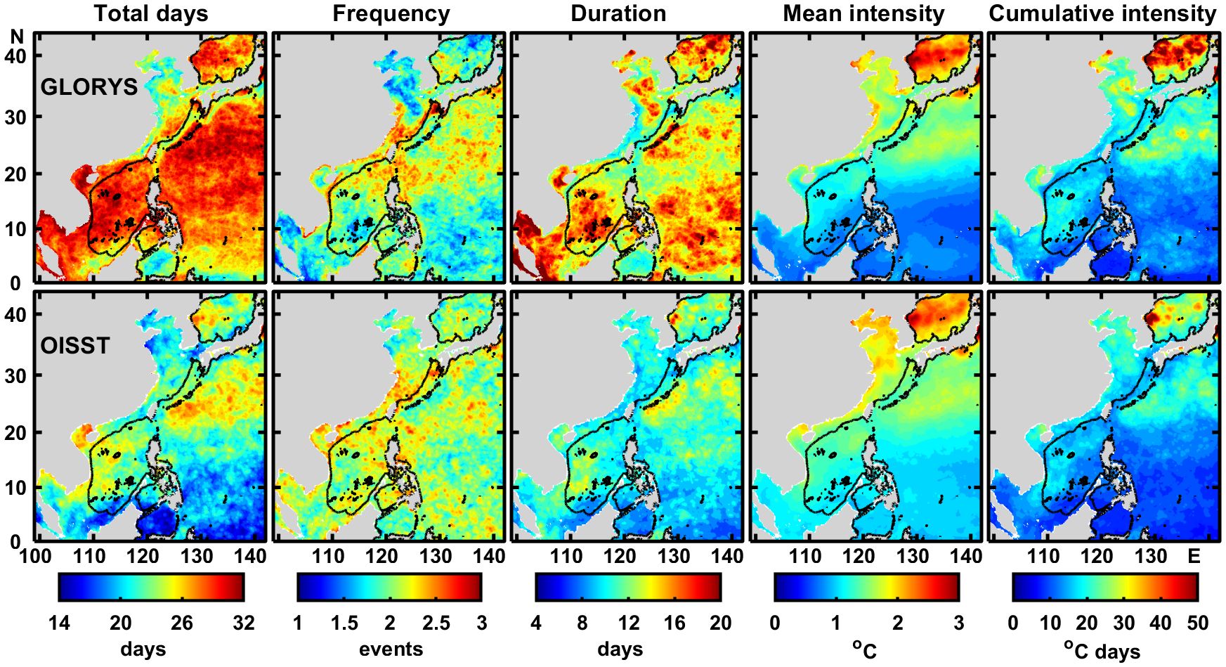
Figure 1 Annual parameters of surface MHWs during 1993–2019 derived from (upper) GLORYS and (lower) OISST. From left to right: total days, frequency, duration, mean intensity, and cumulative intensity. The black contour is the 200 m isobath. The x-axis is in °E and the y-axis is in °N.

For the mean annual total days, the magnitudes and distributions from OISST during 1993–2019 are similar with that reported by Yao et al. (2020) based OISST during 1982–2018. GLORYS obtains similar spatial distribution but larger values. The total days have high values, around 30 (25) days according to GLORYS (OISST), in the Sea of Japan/East Sea, the subtropical gyre bounded by the Kuroshio, and the SCS. Low values of 20–24 (14–20) days according to GLORYS (OISST) are found in the shelf and coastal seas of China (including the Bohai, Yellow and East China Seas), in the southeastern part of the SCS, and at low latitudes to the east of the Philippines.

For the mean annual frequency, GLOYRS and OISST obtain similar ranges of 1.5–3 per year. Values higher than 2.5 per year are found in patched areas along the coast and shelf break of the East China Sea and in mid-latitude (20–30°N) deep regions. The mean annual duration is 14–18 (10–14) days according to GLORYS (OISST) in the Sea of Japan/East Sea, mid-latitude (20–30°N) deep regions and the central and northwestern SCS. South of 20°N, GLORYS obtains duration values of 14–18 days that are much higher than 6–10 days from OISST. This is because the total days and frequency from GLORYS are significantly higher and lower, respectively, than that from OISST.

For the mean annual intensity, GLORYS and OISST obtain similar highest values of 2–3°C in the Sea of Japan/East Sea, moderate high values around 1.5°C in mid-latitude (20–30°N) deep regions and also in the Bohai and Yellow Seas, and 1–1.5°C in the central and northern SCS. South of 20°N to the east of the Philippines and also in the southwestern and southeastern SCS, GLORYS obtains less than 0.5°C, while OISST obtains 0.5–1°C. For the mean annual cumulative intensity, GLORYS obtains the highest values of around 45°C days in the central Sea of Japan/East Sea, 25–30°C days in mid-latitude (20–30°N) deep regions, 15–20°C days in central and northern SCS, and also 5–15°C days in the southwestern SCS and south of 20°N to the east of the Philippines. By comparison, OISST obtains 35, 20–25, 15–20 and less than 10°C days in these regions respectively.

3.2 Inter-annual variations of the mean annual MHW parameters

Based on the values of the MHW parameters for each year, their standard deviations (STDs) are calculated. The resulting spatial distributions of these STDs and the relative magnitudes between the GLORYS and OISST (Figure 2) show similarity with that for the mean annual values for each parameter (Figure 1). Inter-annual variations of the MHW parameters in five representative regions (i.e., the Yellow Sea, the Sea of Japan/East Sea, near the mid-latitude Kuroshio, central SCS, and low-latitude NWP) are presented as time series (Figure 3). GLORYS and OISST obtain overall consistent interannual variations except for the duration, mean intensity and accumulative intensity in the Yellow Sea and the Sea of Japan/East Sea.

Figure 2

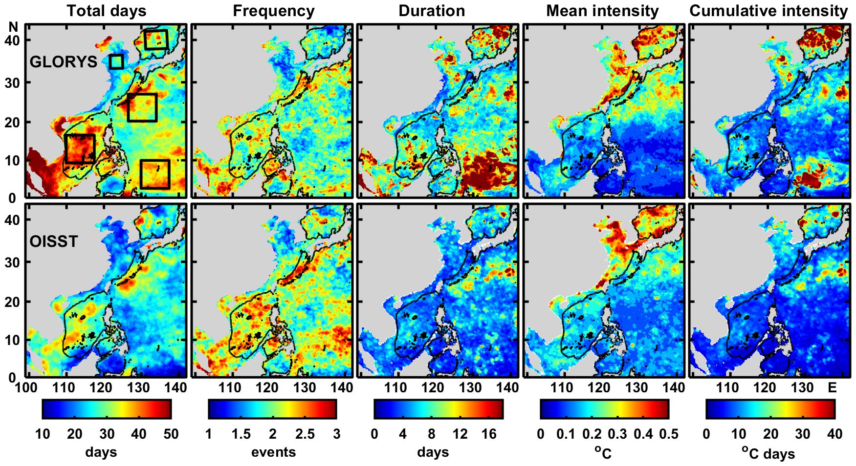
Figure 2 Standard deviations of inter-annual variations of MHW parameters during 1993–2019 derived from (upper) GLORYS and (lower) OISST. From left to right: total days, frequency, duration, mean intensity, and cumulative intensity. The black contour is the 200 m isobath. The five boxes in top-left panel outline the regions for examining the MHW time variations. The x-axis is in °E and the y-axis is in °N.

Figure 3

Figure 3 Time series of annual MHW parameters derived from GLORYS (red curves) and OISST (blue curves), for five representative regions outlines in top-left panel in Figure 2. From left to right: Yellow Sea, Sea of Japan/East Sea, Kuroshio, central South China Sea, and low-latitude NWP. From top to bottom: total days, frequency, duration, mean intensity, and cumulative intensity.

In the region near mid-latitude Kuroshio (Figure 3, third column), four MHW parameters (except the mean intensity) show outstanding peak values found in 1998 and 2015–2017, and moderate peak values in 2001, 2008, 2010 and 2019. In the central SCS (fourth column), outstanding peak values of the four parameters are found in 1998, 2010 and 2014–2016, and moderate peaks in 2001, 2007 and 2019. In low-latitude NWP (fifth column), outstanding peaks in three parameters (total days, frequency and duration) are found in 1998, 2010–2011 and 2016–2018, and moderate peaks in 2013–2014. For the cumulative intensity, outstanding peaks are found in 1998 and 2011. Thus, most peaks values of the four MHW parameters (except mean intensity) in the above three regions are found in common years. In 1998, all the five parameters show peak values in the three regions. The other two regions show different inter-annual variations. In the Sea of Japan/East Sea (second column), peak values of nearly all the five parameters are found in 1994, 1998, 2003–2004, 2008, 2010, 2012–2013, 2017 and 2019. These peak values are mostly moderate according to OISST, but GLORYS obtains some outstanding peak values for the duration and accumulative intensity. In the Yellow Sea (first column), peak values of the five parameters are mostly found in 1994, 1998, 2002, 2004, 2006–2007, 2009–2010, 2012–2013 and 2016–2018.

In order to understand the differences in the MHW parameters derived from different data products, we present in Figure 4 the daily time series of SST and the MHW detection from GLORYS, OISST and CFS in 1998 at two sites, located at the center of the mid-latitude Kuroshio and low-latitude NWP boxes, respectively. At the site in mid-latitude Kuroshio, GLORYS shows the weakest high-frequency fluctuations and detects 7 MHW events, including one long event lasted 30 days during May 1 – May 30, and another one lasted 56 days during August 5–September 29. OISST shows stronger high-frequency fluctuations and detects 9 MHW events, including the one lasted 18 days during May 2– May 19 and the other one lasted 13 days in September. CFS detects five MHW events, including one lasted 18 days in May and another one lasted 13 days in September. In 1998, the accumulative intensity is 30, 19 and 25 °C days according to GLORYS, OISST and CFS.

Figure 4

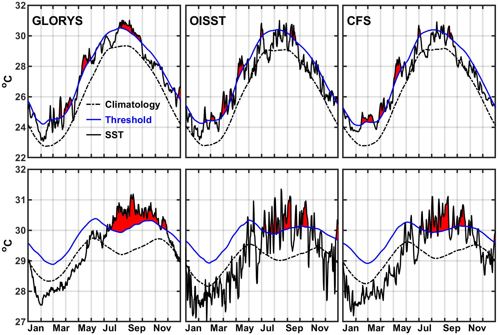
Figure 4 Evolution of MHWs (red shaded) in 1998 indicated by daily SST (black solid line), seasonal climatology (black dotted line), and 90th percentile threshold (blue solid line) at the center of (upper) Kuroshio and (lower) low-latitude NWP. From left to right: GLORYS, OISST, and CFS.

At the site in low-latitude NWP, it is more evident that GLORYS shows the weakest variations at periods up to 2 months (confirmed with spectral analysis, figures not shown). As a result, GLORYS shows continuous warm anomalies and includes only two MHW events during July–November, lasting 118 and 13 days, respectively. In OISST, the presence of strong SST fluctuations leads to 7 MHW events, with durations of 5–18 days. CFS detects four MHW events during July–October with durations of 6–50 days. For this year, the accumulative intensity is 74, 14 and 25 °C days according to GLORYS, OISST and CFS.

Beyond the time scales of MHWs, Figure 4 shows that SST variations from OISST, GLORYS and CFS well follow each other. This is expected because the GLORYS and CFS are produced using realistic atmospheric forcing, and also extensive assimilation of observational data (including the satellite remote sensing SST) that corrects large-scale bias. However, higher frequency SST variations are the weakest in GLORYS and strongest in OISST, with the CFS lying in between. The differences among the three datasets are more evident in low-latitude NWP than in mid-latitude Kuroshio. These differences are possibly due to the noises inherent in OISST, and the different data assimilation approaches used for producing GLORYS and CFS. We suggest further investigation on the causes of these differences, e.g., using in situ SST observations from sea surface buoys.

3.3 Space and interannual variations of the mean seasonal MWH total days and intensity during 1993–2019

Because the five MWH parameters are not totally independent, the following analyses will focus on two parameters, i.e., the total days and the mean intensity. Figure 5 shows the spatial distributions of the MHW total days in different seasons, defined as spring (March to May), summer (June to August), autumn (September to November) and winter (December and the following January and February). According to GLORYS (Figure 5, upper row), in summer the values larger than 7 days are found over the largest areas in both the shelf and deep waters. In autumn, the values are reduced to around 6 days in the Bohai, Yellow and the northern part of the East China Seas. In winter the values are reduced to around 6 days in the northeastern South China Sea. Spring has the smallest areas with values higher than 7 days. The seasonal MHW total days from OISST (Figure 5, lower panel) show broadly similar large-scale spatial distribution with that from GOLORYS, while the values are generally less than 7 days. For the MHW mean intensity, overall the spatial distributions for all the four seasons (Figure 6) are similar with that for the annual mean (Figure 1, fourth column), and GLORYS and OISST show consistent results. Evident seasonal variations are found in the Sea of Japan/East Sea, where the highest values of 3°C are found in the central region in winter, and values of about 2.5°C cover the whole area in summer; and also in the Bohai and Yellow Seas, where the values are the highest in summer (> 2°C according to OISST) followed by spring. In the Yellow Sea, in both spring and summer OISST obtains higher mean intensity values than GLORYS.

Figure 5

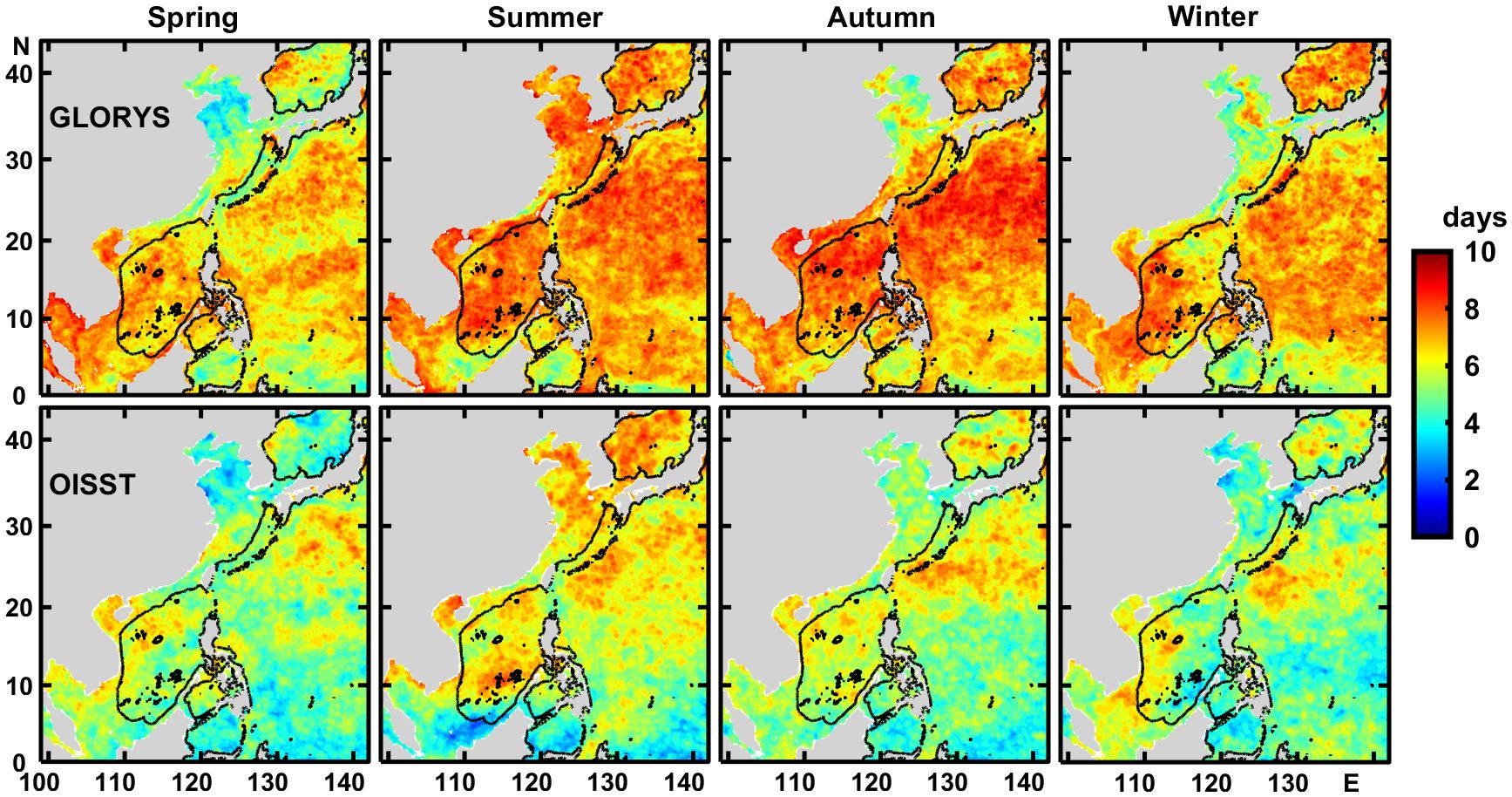
Figure 5 Seasonal total days of surface MHWs during 1993–2019 derived from (upper) GLORYS and (lower) OISST. From left to right: spring, summer, autumn, and winter. The black contour is the 200 m isobath. The x-axis is in °E and the y-axis is in °N.

Figure 6

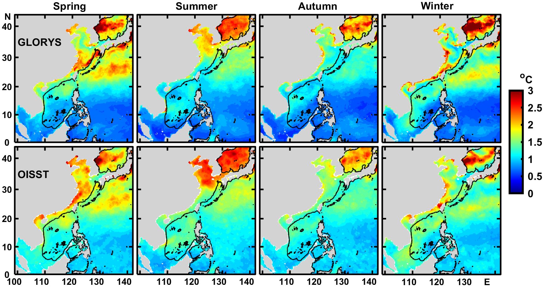
Figure 6 Seasonal mean intensity of surface MHWs during 1993–2019 derived from (upper) GLORYS and (lower) OISST. From left to right: spring, summer, autumn, and winter. The black contour is the 200 m isobath. The x-axis is in °E and the y-axis is in °N.

Next, we examine the interannual variations of the MHW total days and mean intensity, in different seasons at the five representative regions. For the MHW total days (Figure 7), over all GLORYS and OISST obtain peak values in same years for all the regions, with some differences in actual values. For a particular region, some years get a peak value in one season only, while some years get peak values in more than one seasons. For example, in the Yellow Sea (first column), peak values show up in autumn and winter of 2006 and the following spring of 2007. In the central South China Sea (forth column), peak values are found in winter of 1997 and the following three seasons of 1998. Note that for each region, the MHW total days can be zero in some seasons of some years. This results in missing values of the mean MHW intensity (Figure 8). Similar as the annual values (Figure 3, fourth row), GLORYS and OISST obtain consistent interannual variations of mean intensity in each season for the three deep regions of mid-latitude Kuroshio, the central South China Sea, and low-latitude NWP, while evident differences in the Yellow Sea and Sea of Japan/East Sea.

Figure 7

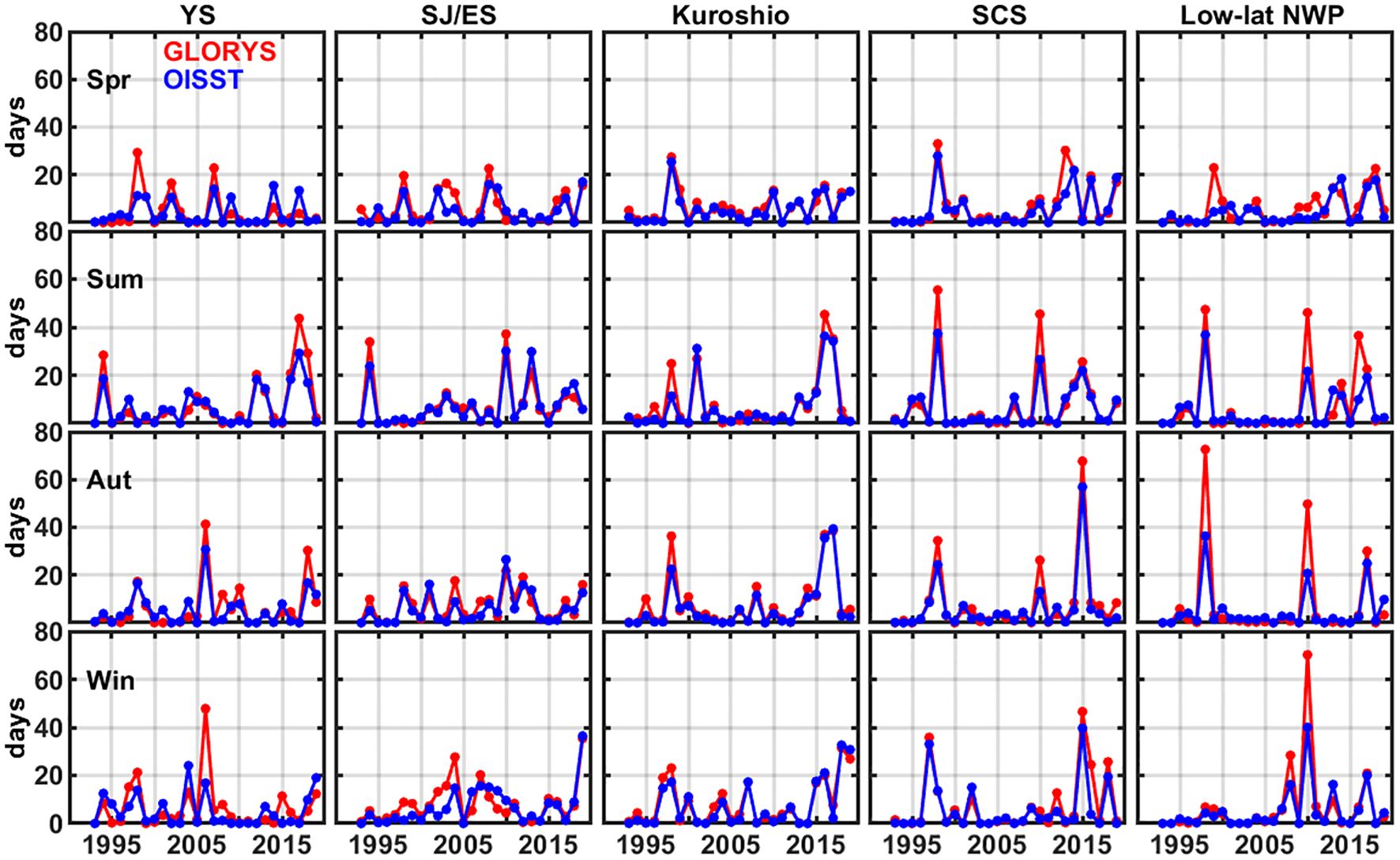
Figure 7 Time series of seasonal MHW total days derived from GLORYS (red curves) and OISST (blue curves), for five representative regions outlines in top-left panel in Figure 2. From left to right: Yellow Sea, Sea of Japan/East Sea, Kuroshio, central South China Sea, and low-latitude NWP. From top to bottom: spring, summer, autumn, and winter.

Figure 8

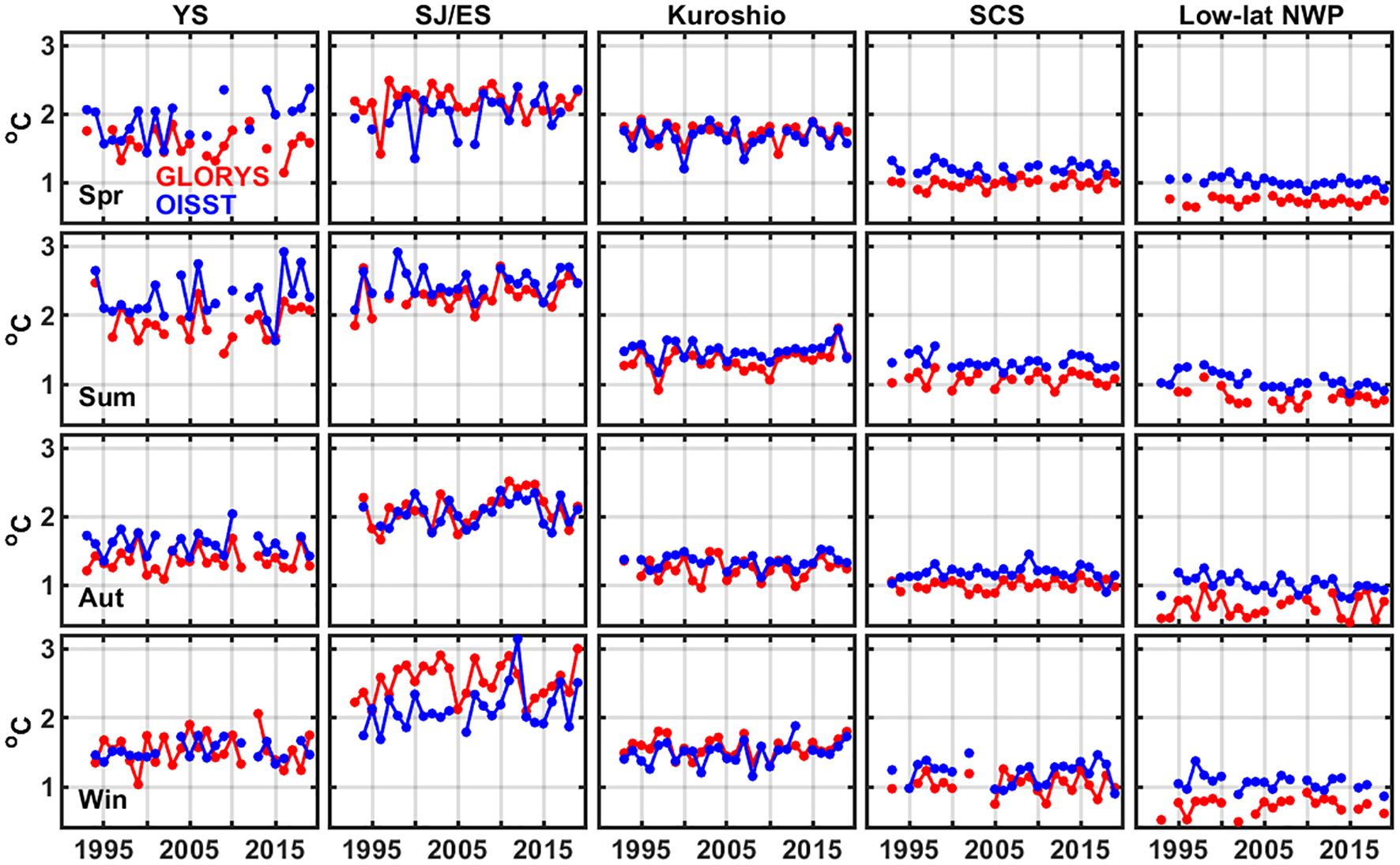
Figure 8 Time series of seasonal MHW mean intensity derived from GLORYS (red curves) and OISST (blue curves), for five representative regions outlines in top-left panel in Figure 2. From left to right: Yellow Sea, Sea of Japan/East Sea, Kuroshio, central South China Sea, and low-latitude NWP. From top to bottom: spring, summer, autumn, and winter.

3.4 Relationship of MHW total days and mean intensity with interannual variations of SST

In this subsection, we examine whether the interannual variations of the MHW total days and mean intensity can be related to the variations of SST. Figure 9 presents the SST anomalies for the annual mean and in each season for the five regions. First, variations of the anomalies from GLORYS and OISST agree well with each other, contrast to the more evident differences in the MHW parameters. Visual inspection indicates that the SST variations show good correspondence with that of the MHW total days, for either the annual means or different seasons, in each of the five regions. In fact, the occurrences of high SST anomalies in one season or in several adjacent seasons in a particular region also show correspondence with the peak values of the MHW total days as discussed at the end of section 3.3. For example, both high SST anomalies and MHW total days occur in the central YS in autumn and winter of 2006 and the spring of 2007, and in the central SCS in winter of 1997 and the following three seasons of 1998. Tables 1A, B confirm that there are significantly positive correlations between interannual variations of the MHW total days and the SST anomalies in all of the five regions, and the correlation values are similar based on either the GLORYS or OISST data.

Figure 9

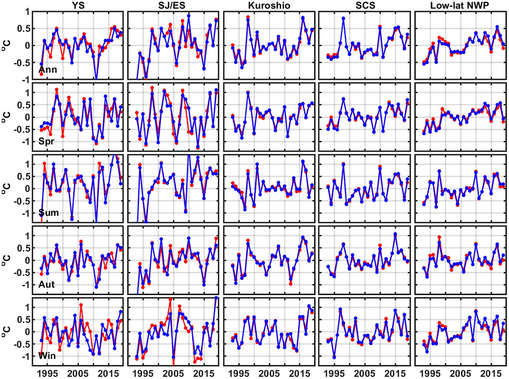
Figure 9 Time series of sea surface temperature anomalies derived from GLORYS (red curves) and OISST (blue curves), for five representative regions outlines in top-left panel in Figure 2. From left to right: Yellow Sea, Sea of Japan/East Sea, Kuroshio, central South China Sea, and low-latitude NWP. From top to bottom: annual, spring, summer, autumn, and winter.

Table 1

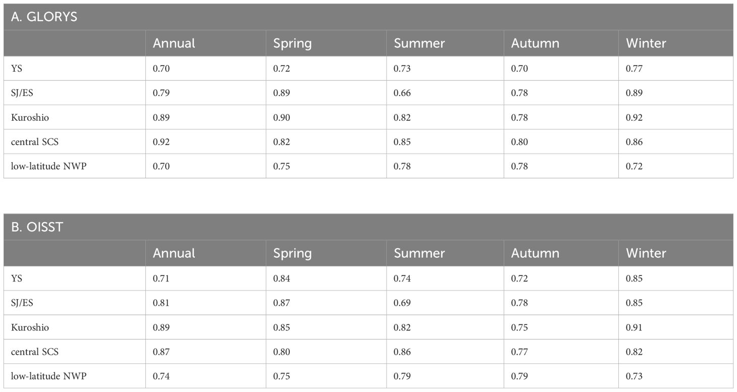
Table 1 Correlation coefficients between interannual variations of the MHW total days and the SST anomalies (p<0.05), for five representative regions outlined in top-left panel in Figure 2.

Tables 2A, B show that correlations between interannual variations of the MHW mean intensity and the SST anomalies are significant only in some seasons in each region, and the results from the two datasets can vary. For example, in the mid-latitude Kuroshio region, significant correlations are found in spring and winter according to GLORYS, while for the annual mean and all the four seasons according to OISST. In the low-latitude NWP, significant correlations are found for the annual mean and three seasons (except spring) according to GLORYS, while are not found at all according to OISST.

Table 2

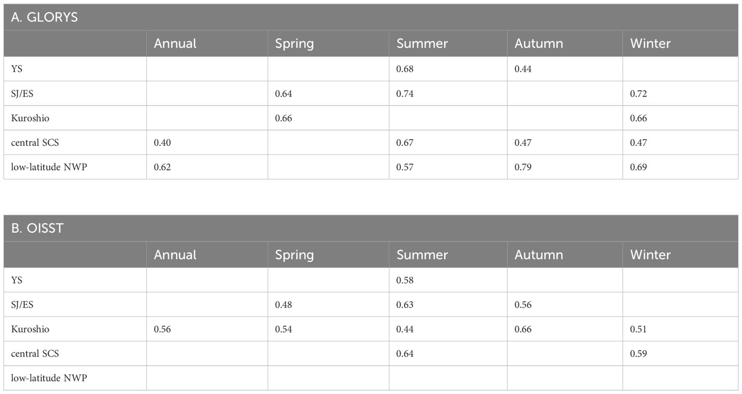
Table 2 Same as Table 1 but for the MHW mean intensity.

3.5 Relationship of MHW total days with variations of the large-scale atmosphere-ocean indices

Compared with the MHW mean intensity, interannual variations of the MHW total days show more established correlation with the SST anomalies. In the following we focus on examining the relationship between the MHW total days and the large scale atmosphere-ocean indices. Figure 10 presents the interannual variations of these large-scale atmosphere-ocean indices as introduced in section 2.4. For the Aleutian Low index, only the winter-mean values are shown. For the Niño3.4 index, only the annual mean (averaged over January – December) values are used. This is because the interannual variability of the Niño3.4 index is robustly phase-locked to the seasonal cycle, i.e., the Niño3.4 index can be quite accurately reproduced by the product between a seasonal structure and the time series of annual amplitude (e.g., Clarke, 2014). For all the other indices, the seasonal-mean values for each season are presented. The East Asia Monsoon intensity in each season (third column) is the average of absolute monthly values. Note that the monsoon wind is southwesterly in summer and northeasterly in winter (denoted as EASM and EAWM, respectively), and can have fluctuating directions in spring and autumn. Figures 11, 12 display the spatial distributions of the correlation coefficients between each of the above indices with the MHW total days derived from GLORYS. The correlations between the indices and the MHW total days derived from OISST are similar (Figures not shown).

Figure 10

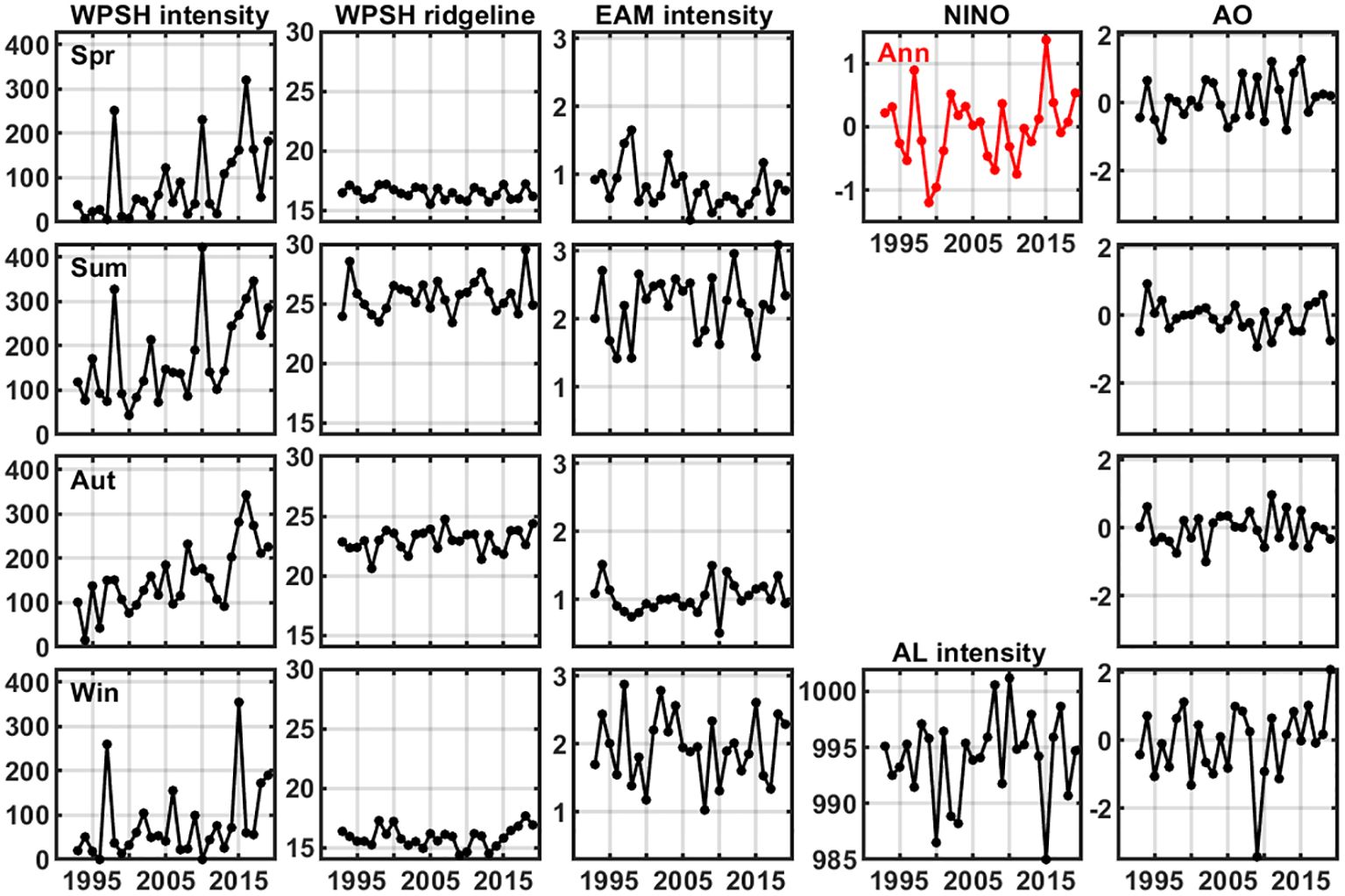
Figure 10 Time series of the large-scale atmosphere-ocean indices relevant to the Northwest Pacific region. From left to right: WPSH intensity, WPSH ridgeline, EAM intensity, Niño3.4/AL intensity, and AO. From top to bottom: seasonal-mean values for spring, summer, autumn, and winter, except for the annual-mean for the Niño3.4 index (red curve).

Figure 11

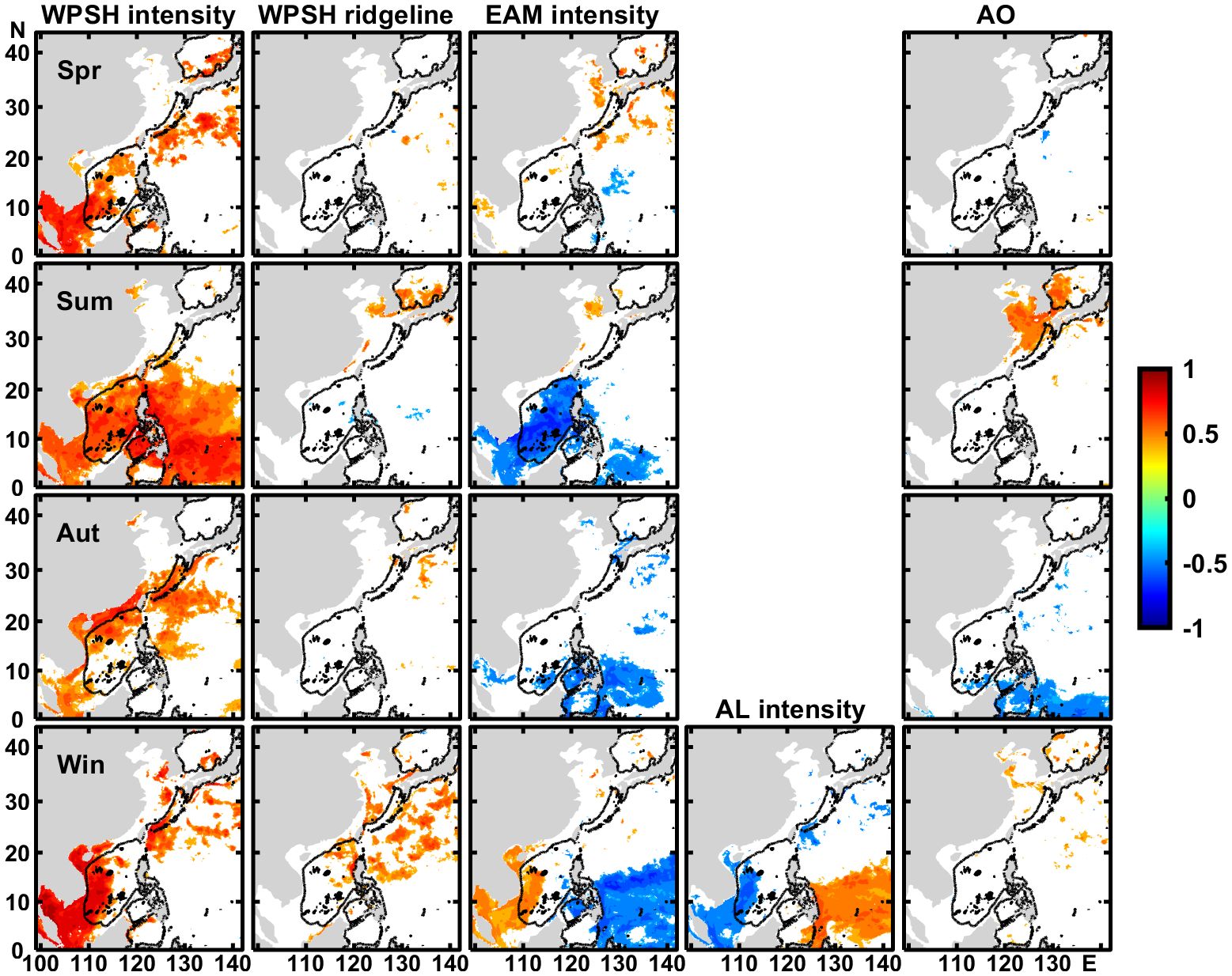
Figure 11 Spatial distributions of the correlation coefficients between variations of the MHW total days at different locations derived from GLORYS and the interannual variations of large-scale atmosphere-ocean indices. i.e., from left to right: the WPSH intensity, WPSH ridgeline, EAM intensity, AL intensity in winter, and AO. From top to bottom: spring, summer, autumn, and winter. The color shading shows the correlation coefficients with a confidence level greater than 95%. The x-axis is in °E and the y-axis is in °N.

3.5.1 Western Pacific Subtropical High

The WPSH intensity has positive correlations (p<0.05) with the MHW total days, over different regions in different seasons (Figure 11, first column). The areas with significant correlations are over the western half of the SCS in winter, shrink to the southwestern SCS in spring, and expand to cover nearly the whole SCS and the deep NWP south of 20°N in summer. In Autumn, positive correlations are found over the shelf seas of the northern SCS and the East China Sea, and within 20–30°N near the Kuroshio. The high correlations are related to the occurrences of dominant peaks in the WPSH intensity and MHW total days in specific regions, for example in summer of 1998, 2010 and 2013–2016 in the central SCS and low-latitude NWP, and in winter of 1997 and 2015 in the central SCS which also covers a significant part of the western SCS. The WPSH ridgeline overall has no significant correlation with the MHW total days, except over the southern Sea of Japan/East Sea in summer and at scattered locations extending from the eastern SCS to the mid-latitude Kuroshio region in winter (Figure 11, second column). The time series of the WPSH ridgeline (Figure 10, second column) show no outstanding peaks except for a few moderate ones in summer.

3.5.2 East Asia Monsoon

The East Asia Summer Monsoon intensity has negative correlations with the MHW total days over nearly the whole SCS (Figure 11, third column). The EASM intensity show low values in 1995, 1996, 1998, 2007, 2010 and broadly in 2013–2017, while the MHW total days in the SCS show high values during most of these years in summer. The East Asia Winter Monsoon intensity has negative and positive correlations with the MHW total days in low-latitude NWP and western SCS, respectively. In the low-latitude NWP, the MHW total days show outstanding peak values in 2008, 2010, 2013 and 2017, when the EAWM intensity also shows low values. In the SCS, the MHW total days show outstanding peak values in 1997, 2015 and 2018, when the EAWM intensity also shows high values. In autumn, negative correlations are found within 0–10°N, covering much smaller areas than in summer and winter.

3.5.3 Aleutian Low

In winter, the AL intensity has positive and negative correlations with the MHW total days in low-latitude NWP and western SCS, respectively (Figure 11, forth column). In the western SCS, the negative correlation is directly opposite to the positive correlation with the WPSH intensity. In fact, in winter the AL and WPSH intensities have a negative correlation of r=-0.56 (p<0.05). The AL intensity has significantly low values in 1997, 2000, 2002, 2003, 2015 and 2018, while the WPSH intensity shows outstanding peaks in 1997, 2015, 2017 and 2018. In the low-latitude NWP, the positive (negative) correlations with the AL intensity (EAWM intensity) are also opposite. The AL and EAWM intensities have a negative correlation of r=-0.57 (p<0.05).

3.5.4 Arctic Oscillation

Significant correlations between the AO index and MHW total days are only found as being positive in the Yellow Sea and western Sea of Japan/East Sea in summer, and as being negative in low-latitude NWP in autumn (Figure 11, fifth column). In summer, the AO index shows high values in 1994, 2010, 2012–2013 and 2016–2018 (Figure 10. fifth column), while the MHW total days in the Yellow Sea show outstanding peaks in 1994, 2012–2013 and 2016–2018 (Figure 7, first column). Correspondingly, the WPSH ridgeline in summer is positively correlated with the AO index (r=0.42, p<0.05). Interestingly despite of the AO index’s strong variations in winter, it has no significant correlation with the MHW total days even in the northern regions of the NWP.

3.5.5 ENSO

Figure 12 show the correlations between the annual-mean Niño3.4 index and the of MHW total days in different seasons, from the corresponding years (upper row) or delayed by one year (lower row). Significantly positive correlations are found 1) with the MHW total days in autumn and winter (denoted by the text of “Aut” and ‘Win”) of the corresponding years over the western half of SCS, and 2) with the MHW total days delayed by one year in spring (denoted by “Spr+1”) over the southwestern SCS and mid-latitude Kuroshio region, in summer (denoted by “Sum+1”) over the largest areas including the whole SCS, low-latitude NWP, and the mid-altitude Kuroshio region; and in Autumn (denoted by “Aut+1”) in low-latitude NWP and mid-altitude Kuroshio region.

Figure 12

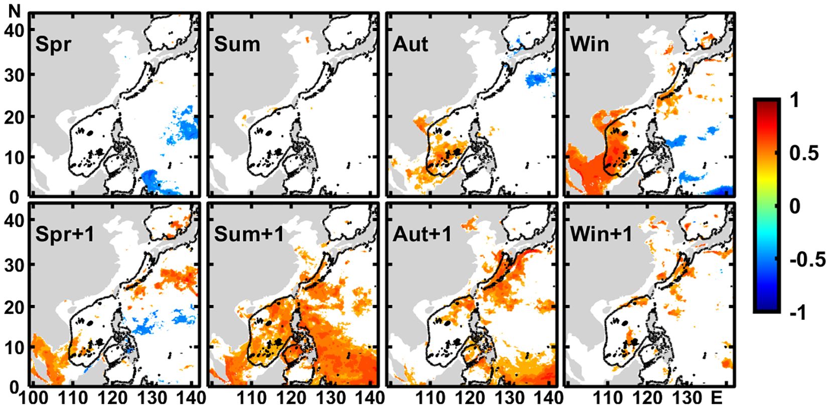
Figure 12 Similar as Figure 11 but for the correlation coefficients between time series of the annual-mean Niño3.4 index and the MHW total days in (from left to right) spring, summer, autumn, and winter, (upper row) without and (lower row) with the lag by one year. The x-axis is in °E and the y-axis is in °N.

4 Discussion and conclusion

Five surface MHW parameters in the NWP during 1993–2019 are derived from two SST datasets, namely OISST V2.1 based on satellite remote sensing and that from a global ocean data assimilative product GLORYS12V1. For the annual values of these parameters, analyses of the two SST datasets obtain similar spatial distributions averaged during 1993–2019, consistent with previous studies (e.g., Yao et al., 2020). The MHW total days and duration from GLORYS are usually higher than that from OISST, which can be attributed to the differences between the two SST datasets in terms of the accuracies and noises. The standard deviations of these MHW parameters show similar spatial distributions with that of the mean annual values for each parameter. In five selected representative regions, interannual variations of the MHW total days, frequency, duration and cumulative intensity show outstanding peak values in certain years. The spatial and temporal variations of the five mean annual MWH parameters are not totally independent. The parameter of MHW total days is close to the product of frequency and duration, while the cumulative intensity is close to the product of total days and mean intensity. Focusing on the seasonal MHW total days and mean intensity, their spatial distributions and interannual variations from the two datasets are also similar.

In each representative region, interannual variations of the MHW total days have significantly positive correlations with the SST anomalies, for both the annual and seasonal means. By comparison, less established are the correlations between interannual variations of the MHW mean intensity and the SST anomalies, which are significant only in some seasons in each region. The correlation analyses between interannual variations of the MHW total days and the large-scale indices for the atmosphere-ocean circulation of relevance to the NWP are carried out. The following results are obtained and interpreted with the relationships between the SST variations and these indices, as well as the relationships among these indices with reference to the findings of previous studies.

First, the correlations between the interannual variations of the MHW total days at different locations for each season and the seasonal indices of the Western Pacific Subtropical High intensity and ridgeline, the East Asia Monsoon intensity, the Aleutian Low intensity and the Arctic Oscillation are computed. In summer, the MHW total days have significantly positive correlations with the WPSH intensity, and negative correlations with the EAM intensity, over nearly the whole SCS and in low-latitude NWP. This is consistent with the negative correlation of r=-0.35 (insignificant at p<0.05) between the two indices. In winter, the MHW total days have significantly positive correlations with both the WPSH and EAM intensities over the western part of SCS, consistent with the positive correlation of r=0.63 (p<0.05) between the two winter indices. The MHW total days overall have no significant correlations with the WPSH ridgeline. In winter, the MHW total days have positive and negative correlations with the Aleutian Low intensity in low-latitude NWP and western SCS, respectively. The Arctic Oscillation index is positively correlated with the MHW total days in the Yellow Sea and western Sea of Japan/East Sea in summer, while negatively correlated in low-latitude NWP in autumn.

The above identified relationships among the MHW total days, WPSH and EAM are consistent with previous findings. In summer, the strengthening and westward extension of the WPSH can cause strong descending motions and contributed considerably to the surface warming in the NWP (Wang et al., 2019). The same changes of the WPSH also favor the generation of anticyclones which bring easterly wind anomalies to low latitudes and weaken the EASM south of 12°N in the SCS. The resulting negative anomaly of the wind stress curl causes the weakening or even disappearance of upwelling in midwestern SCS, causing severe MHWs across the SCS in summer (Yao and Wang, 2021). During1993–2019, the negative correlations between the summer MHW total days and the EASM intensity are consistent with the conclusions of previous studies at the interdecadal variations. Cai et al. (2017) identified distinct variations of robust surface warming in the NWP region (referred to as “offshore area of China”) in both summer and winter during 1958–2014. They revealed that the acceleration of warming during 1980–1999 was accompanied by a weakening of the EAM and a strengthening of the WPSH. Interdecadal variations of SST and EAM wind were well correlated. In both summer and winter, the weakening of the leading EOF (Empirical Orthogonal Function) mode of EAM wind could enhance the flow of Kuroshio Current into the SCS through the Luzon Strait, and this oceanic lateral heat transfer played a central role in surface warming in the northern SCS. In summer, except for the effect of oceanic lateral heat transfer, surface warming can also be caused by the increased surface radiative heating associated with the strengthening of the third EOF mode of EAM anticyclone wind (i.e., WPSH).

Next, the correlations are computed between the annual-mean Niño3.4 index and the MHW total days in different seasons from the corresponding years and delayed by one year. Overall, the analyses results suggest that the occurrence of strong El Niño will be followed by longer MHW total days in winter of the present year over the western half of the SCS, and in the next year in spring over the southwestern SCS and mid-latitude Kuroshio region, in summer over the largest areas including the whole SCS, low-latitude NWP, and the mid-altitude Kuroshio region, and in Autumn in low-latitude NWP and mid-altitude Kuroshio region. This result suggests the possibility to predict the MHW total days in the NWP using the Niño3.4 index with the lead time of several seasons. The causes of this identified predictability must be related to the phase relationship between the Niño3.4 index with the SST changes in the NWP, that has been documented in many previous studies (e.g., Wang et al., 2020a, Wang et al., 2020b).

The seasonal MHW total days show similar spatial distributions of correlations with the seasonal WPSH intensity and the annual Niño3.4 index. This is related to the high correlations between the two indices, with the annual Niño3.4 index leading the WPSH intensity (and also the MHW total days) by several seasons. The annual Niño3.4 index and the winter WPSH intensity have a significant correlation of r=0.76 (p<0.05). Both indices, as well as the winter MHW total days in the central SCS show outstanding peaks in 1997 and 2015 (i.e., strong El Niño years). Note that the annual Niño3.4 index is the average over January–December from the same years, while the winter WPSH intensity is averaged from December to January–February of next year. Furthermore, the annual Niño3.4 index (winter WPSH intensity) has positive correlations of r=0.70 (0.81), 0.64 (0.58) and 0.45 (0.48) (p<0.05) with the time series of the WPSH intensity delayed by one year in spring, summer and autumn, respectively. These correlations are consistent with the previous findings. For example, Wu et al. (2017) and Zou et al. (2017) revealed that the positive Niño3.4 index in winter strengthens the WPSH in the following spring and summer.

We note that during 1993–2019, the time series of the MHW total days and nearly all of the indices of atmosphere-ocean circulation (except the WPSH ridgeline) show outstanding peaks in certain years. Hence, the correlations identified and discussed above are dominated by these peak values. This means that these correlation relationships can be mainly used to understand and predict the occurrence of significant MHW events (with prolonged MHW total days). In practice, significant MHWs usually raise the most concerns because of their potentially severe impacts on marine ecosystems and fishery.

The consistency in the surface MHW parameters derived from OISST and suggests that either dataset can be used to study the space-time variations of the MHW parameters. It is encouraging to further analyze the state-of-the-art ocean model solutions for quantifying and studying the MHWs in the water column and near the seabed that are of more relevance to ecosystem and fishery. However, there are always needs to validate the model solutions with observational data, understand the causes of model biases and work on improving the models. For example, the significant differences between GLORYS and OISST in low-latitude NWP, in terms of SST variations and MHW parameters (Figure 4), require further investigation. Finally, further studies are needed to link the space and time variations of MHW parameters to variations of ecological variables (i.e., chlorophyll, dissolved oxygen, primary productivity) for addressing the important issues in marine ecosystem and environment under the multi-scale climate change.

Data availability statement

The original contributions presented in the study are included in the article/supplementary material. Further inquiries can be directed to the corresponding author.

Author contributions

HW: Writing – original draft. YL: Writing – original draft. LZ: Writing – original draft. XC: Writing – review & editing. SL: Writing – review & editing.

Funding

The author(s) declare financial support was received for the research, authorship, and/or publication of this article. This study was initiated while HW was visiting the Bedford Institute of Oceanography, Canada, with support from the China Scholarship Council. Additional work of HW, XC, and SL was funded by the Natural Science Foundation of China (42192561 and 41907180), National Key R&D Program of China (2020YFA0608804), and Key Laboratory of Space Ocean Remote Sensing and Application (Ministry of Natural Resources) Open Research program (202101001). YL and LZ acknowledge Fisheries and Oceans Canada for support in terms of research time, facility and management.

Acknowledgments

We thank the reviewers for insightful and constructive comments that helped to improve the analysis and presentation of this study.

Conflict of interest

The authors declare that the research was conducted in the absence of any commercial or financial relationships that could be construed as a potential conflict of interest.

Publisher’s note

All claims expressed in this article are solely those of the authors and do not necessarily represent those of their affiliated organizations, or those of the publisher, the editors and the reviewers. Any product that may be evaluated in this article, or claim that may be made by its manufacturer, is not guaranteed or endorsed by the publisher.

References

Amaya D. J., Miller A. J., Xie S., Kosaka Y. (2020). Physical drivers of the summer 2019 North Pacific marine heatwave. Nat. Commun. 11, 1903. doi: 10.1038/s41467-020-15820-w

PubMed Abstract | CrossRef Full Text | Google Scholar

Banzon V., Smith T. M., Chin T. M., Liu C., Hankins W. (2016). A long-term record of blended satellite and in situ sea-surface temperature for climate monitoring, modeling and environmental studies. Earth Syst. Sci. Data 8, 165–176. doi: 10.5194/essd-8-165-2016

CrossRef Full Text | Google Scholar

Cai R., Tan H., Kontoyiannis H. (2017). Robust surface warming in offshore China seas and its relationship to the East Asian monsoon wind field and ocean forcing on interdecadal time scales. J. Climate 30, 8987–9005. doi: 10.1175/JCLI-D-16-0016.1

CrossRef Full Text | Google Scholar

Carvalho K. S., Smith T. E., Wang S. (2021). Bering Sea marine heatwaves: Patterns, trends and connections with the Arctic. J. Hydrol. 600, 126462. doi: 10.1016/j.jhydrol.2021.126462

CrossRef Full Text | Google Scholar

Clarke A. J. (2014). El Niño physics and El Niño predictability. Annu. Rev. Mar. Sci. 6, 79–99. doi: 10.1146/annurev-marine-010213-135026

CrossRef Full Text | Google Scholar

Drévillon M., Fernandez E., Lellouche J. M. (2022). Global ocean physics reanalysis: GLOBAL_MULTIYEAR_PHY_001_030. CMEMS. doi: 10.48670/moi-00021

CrossRef Full Text | Google Scholar

Favoretto F., Sánchez C., Aburto-Oropeza O. (2022). Warming and marine heatwaves tropicalize rocky reefs communities in the Gulf of California. Prog. Oceanogr. 206, 102838. doi: 10.1016/j.pocean.2022.102838

CrossRef Full Text | Google Scholar

Gao G., Marin M., Feng M., Yin B., Yang D., Feng X., et al. (2020). Drivers of marine heatwaves in the East China Sea and the South Yellow Sea in three consecutive summers during 2016–2018. J. Geophys. Res.-Oceans 125, e2020JC016518. doi: 10.1029/2020JC016518

CrossRef Full Text | Google Scholar

Hobday A. J., Alexander L. V., Perkins S. E., Smale D. A., Straub S. C., Oliver E. C. J., et al. (2016). A hierarchical approach to defining marine heatwaves. Prog. Oceanogr. 141, 227–238. doi: 10.1016/j.pocean.2015.12.014

CrossRef Full Text | Google Scholar

Holbrook N. J., Hernaman V., Koshiba S., Lako J., Kajtar J. B., Amosa P., et al. (2022). Impacts of marine heatwaves on tropical western and central Pacific Island nations and their communities. Global Planet. Change 208, 103680. doi: 10.1016/j.gloplacha.2021.103680

CrossRef Full Text | Google Scholar

Huang B., Liu C., Banzon V., Freeman E., Graham G., Hankins B., et al. (2021a). Improvements of the daily optimum interpolation sea surface temperature (DOISST) version 2.1. J. Climate 34, 2923–2939. doi: 10.1175/JCLI-D-20-0166.1

CrossRef Full Text | Google Scholar

Huang B., Wang Z., Yin X., Arguez A., Graham G., Liu C., et al. (2021b). Prolonged marine heatwaves in the Arctic: 1982–2020. Geophys. Res. Lett. 48, e2021GL095590. doi: 10.1029/2021GL095590

CrossRef Full Text | Google Scholar

Huang Z., Feng M., Beggs H., Wijffels S., Cahill M., Griffin C. (2021c). High-resolution marine heatwave mapping in Australasian waters using Himawari-8 SST and SSTAARS data. Remote Sens. Environ. 267, 112742. doi: 10.1016/j.rse.2021.112742

CrossRef Full Text | Google Scholar

Izquierdo P., Taboada F. G., González-Gi R., Arrontes J., Rico J. M. (2022). Alongshore upwelling modulates the intensity of marine heatwaves in a temperate coastal sea. Sci. Total Environ. 835, 155478. doi: 10.1016/j.scitotenv.2022.155478

PubMed Abstract | CrossRef Full Text | Google Scholar

Jiang M., Gao L., Huang R., Lin X., Gao G. (2022). Differential responses of bloom-forming Ulva intestinalis and economically important Gracilariopsis lemaneiformis to marine heatwaves under changing nitrate conditions. Sci. Total Environ. 840, 156591. doi: 10.1016/j.scitotenv.2022.156591

PubMed Abstract | CrossRef Full Text | Google Scholar

Kalnay E., Kanamitsu M., Kistler R., Collins W., Deaven D., Gandin L., et al. (1996). The NCEP/NCAR 40-year reanalysis project. B. Am. Meteorol. Soc 77, 437–471. doi: 10.1175/1520-0477(1996)077<0437:TNYRP>2.0.CO;2

CrossRef Full Text | Google Scholar

Lellouche J. M., Greiner E., Bourdallé-Badie R., Garric G., Melet. A., Drévillon M., et al. (2021). The copernicus global 1/12° Oceanic and sea ice GLORYS12 reanalysis. Front. Earth Sc-Switz. 9. doi: 10.3389/feart.2021.698876

CrossRef Full Text | Google Scholar

Li D., Chen Y., Qi J., Zhu Y., Lu C., Yin B. (2023a). Attribution of the July 2021 record-breaking northwest Pacific marine heatwave to global warming, atmospheric circulation, and ENSO. B. Am. Meteorol. Soc 104, 291–297. doi: 10.1175/BAMS-D-22-0142.1

CrossRef Full Text | Google Scholar

Li Y., Ren G., Wang Q., Mu L. (2023b). Changes in marine hot and cold extremes in the China Seas during 1982–2020. Weather Clim. Extreme 39, 100553. doi: 10.1016/j.wace.2023.100553

CrossRef Full Text | Google Scholar

Liu Y., Liang P., Sun Y. (2019). The Asian summer monsoon: characteristics, variability, teleconnections and projection (Cambridge, MA: Elsevier), 87.

Google Scholar

Liu K., Xu K., Zhu C., Liu B. (2022). Diversity of marine heatwaves in the South China Sea regulated by ENSO phase. J. Climate 35, 877–893. doi: 10.1175/JCLI-D-21-0309.1

CrossRef Full Text | Google Scholar

Mo S., Chen T., Chen Z., Zhang W., Li S. (2022). Marine heatwaves impair the thermal refugia potential of marginal reefs in the northern South China Sea. Sci. Total Environ. 825, 154100. doi: 10.1016/j.scitotenv.2022.154100

PubMed Abstract | CrossRef Full Text | Google Scholar

Oliver E. C. J., Burrows M. T., Donat M. G., Gupta A. S., Alexander L. V., Perkins-Kirkpatrick S. E., et al. (2019). Projected marine heatwaves in the 21st century and the potential for ecological impact. Front. Mar. Sci. 6. doi: 10.3389/fmars.2019.00734

CrossRef Full Text | Google Scholar

Oliver E. C. J., Donat M. G., Burrows M. T., Moore P. J., Smale D. A., Alexander L. V., et al. (2018). Longer and more frequent marine heatwaves over the past century. Nat. Commun. 9, 1324. doi: 10.1038/s41467-018-03732-9

PubMed Abstract | CrossRef Full Text | Google Scholar

Overland J. E., Adams J. M., Bond N. A. (1999). Decadal variability of the Aleutian Low and its relation to high-latitude circulation. J. Climate 12, 1542–1548. doi: 10.1175/1520-0442(1999)012<1542:DVOTAL>2.0.CO;2

CrossRef Full Text | Google Scholar

Plecha S. M., Soares P. M. M. (2020). Global marine heatwave events using the new CMIP6 multi-model ensemble: from shortcomings in present climate to future projections. Environ. Res. Lett. 15, 124058. doi: 10.1088/1748-9326/abc847

CrossRef Full Text | Google Scholar

Qi R., Zhang Y., Du Y., Feng M. (2022). Characteristics and drivers of marine heatwaves in the western equatorial Indian Ocean. J. Geophys. Res.-Oceans 127, e2022JC018732. doi: 10.1029/2022JC018732

CrossRef Full Text | Google Scholar

Qiu Z., Qiao F., Jang C. J., Zhang L., Song Z. (2021). Evaluation and projection of global marine heatwaves based on CMIP6 models. Deep-Sea Res. Pt II 194, 104998. doi: 10.1016/j.dsr2.2021.104998

CrossRef Full Text | Google Scholar

Reyes-Mendoza O., Manta G., Carrillo L. (2022). Marine heatwaves and marine cold-spells on the Yucatan Shelf-break upwelling region. Cont. Shelf Res. 239, 104707. doi: 10.1016/j.csr.2022.104707

CrossRef Full Text | Google Scholar

Reynolds R. W., Smith T. M., Liu C., Chelton D. B., Casey K. S., Schlax M. G. (2007). Daily high-resolution-blended analyses for sea surface temperature. J. Climate 20, 5473–5496. doi: 10.1175/2007JCLI1824.1

CrossRef Full Text | Google Scholar

Saha S., Moorthi S., Pan H., Wu X., Wang J., Nadiga S., et al. (2010). The NCEP climate forecast system reanalysis. B. Am. Meteorol. Soc 91, 1015–1057. doi: 10.1175/2010BAMS3001.1

CrossRef Full Text | Google Scholar

Saha S., Moorthi S., Wu X., Wang J., Nadiga S., Tripp P., et al. (2014). The NCEP climate forecast system version 2. J. Climate 27, 2185–2208. doi: 10.1175/JCLI-D-12-00823.1

CrossRef Full Text | Google Scholar

Saranya J. S., Roxy M. K., Dasgupta P., Anand A. (2022). Genesis and trends in marine heatwaves over the tropical Indian Ocean and their interaction with the Indian summer monsoon. J. Geophys. Res.-Oceans 127, e2021JC017427. doi: 10.1029/2021JC017427

CrossRef Full Text | Google Scholar

Tan H., Cai R., Wu R. (2022). Summer marine heatwaves in the South China Sea: Trend, variability and possible causes. Adv. Clim. Change Res. 13, 323–332. doi: 10.1016/j.accre.2022.04.003

CrossRef Full Text | Google Scholar

Thompson D. W. J., Wallace J. M. (2000). Annular modes in the extratropical circulation. Part I: month-to-month variability. J. Climate 13, 1000–1016. doi: 10.1175/1520-0442(2000)01360;1000:amitec62;2.0.co;2

CrossRef Full Text | Google Scholar

Varela R., Rodríguez-Díaz L., de Castro M., Gómez-Gesteira M. (2021). Influence of Eastern Upwelling systems on marine heatwaves occurrence. Global Planet. Change 196, 103379. doi: 10.1016/j.gloplacha.2020.103379

CrossRef Full Text | Google Scholar

Wang M., Guo J., Song J., Fu Y., Sui W., Li Y., et al. (2020a). The correlation between ENSO events and sea surface temperature anomaly in the Bohai Sea and Yellow Sea. Reg. Stud. Mar. Sci. 35, 101228. doi: 10.1016/j.rsma.2020.101228

CrossRef Full Text | Google Scholar

Wang S., Jing Z., Wu L., Wang H., Shi J., Chen Z., et al. (2022). Changing ocean seasonal cycle escalates destructive marine heatwaves in a warming climate. Environ. Res. Lett. 17, 054024. doi: 10.1088/1748-9326/ac6685

CrossRef Full Text | Google Scholar

Wang Q., Li Y., Li Q., Liu Y., Wang Y. (2019). Changes in means and extreme events of sea surface temperature in the east China seas based on satellite data from 1982 to 2017. Atmosphere 10, 140. doi: 10.3390/atmos10030140

CrossRef Full Text | Google Scholar

Wang Y., Yu Y., Zhang Y., Zhang H., Chai F. (2020b). Distribution and variability of sea surface temperature fronts in the south China sea. Estuar. Coast. Shelf S. 240, 106793. doi: 10.1016/j.ecss.2020.106793

CrossRef Full Text | Google Scholar

Wu L., Chang J., Xu Y. (2017). Relationship between the spring precipitation in north China and ENSO. Meteorol. Environ. Sci. 40, 21–25. doi: 10.16765/j.cnki.1673-7148.2017.01.003

CrossRef Full Text | Google Scholar

Yao Y., Wang C. (2021). Variations in summer marine heatwaves in the South China sea. J. Geophys. Res.-Oceans 126, e2021JC017792. doi: 10.1029/2021JC017792

CrossRef Full Text | Google Scholar

Yao Y., Wang C., Fu Y. (2022). Global marine heatwaves and cold-spells in present climate to future projections. Earth's Future 10, e2022EF002787. doi: 10.1029/2022EF002787

CrossRef Full Text | Google Scholar

Yao Y., Wang J., Yin J., Zou X. (2020). Marine heatwaves in China's marginal seas and adjacent offshore waters: Past, Present, and Future. J. Geophys. Res.- Oceans 125, e2019JC015801. doi: 10.1029/2019JC015801

CrossRef Full Text | Google Scholar

Zhao Z., Marin M. (2019). A MATLAB toolbox to detect and analyze marine heatwaves. J. Open Source Software 4, 1124. doi: 10.21105/joss.01124

CrossRef Full Text | Google Scholar

Zhu C., He J., Wu G. (2000). East Asian Monsoon index and its interannual relationship with largescale thermal dynamic circulation. Acta Meteorol. Sin. 58, 391–402. doi: 10.3321/j.issn:0577-6619.2000.04.002

CrossRef Full Text | Google Scholar

Zhu C., Lee W.-S., Kang H., Park C.-K. (2005). A proper monsoon index for seasonal and interannual variations of the East Asian monsoon. Geophys. Res. Lett. 32, L02811. doi: 10.1029/2004GL021295

CrossRef Full Text | Google Scholar

Zou M., Qiao S., Wu Y., Feng G. (2017). Effects of anomalous water vapor transport from tropical Indian Ocean-western Pacific on summer rainfall in eastern China. Chin. J. Atmos. Sci. 41, 988–998. doi: 10.3878/j.issn.1006-9895.1702.16232

CrossRef Full Text | Google Scholar