Nodal modulation of M2 and N2 tides along the Norwegian coast

1 Introduction

Greenhouse gas emissions from human activities have imposed numerous adverse impacts on both society and the environment (Kerr, 2007). In the coming decades, regions closer to the equator are expected to see reduced crop yields due to more frequent and severe droughts (Lu et al., 2019). Conversely, areas farther from the equator are likely to experience warmer and wetter climate changes (Milly et al., 2002), potentially leading to increased flooding events and higher sea levels in high latitudes, posing a dramatical threat to coastal residents (Nicholls, 2004). Therefore, it is crucial to focus on sea level fluctuations in high-latitude coastal areas. The melting of sea ice in the Arctic Ocean is happening at an alarming rate due to global warming (Kumar et al., 2020). This has led to a reduction in the reflection of solar radiation, an increase in the absorption of solar radiation, an influx of freshwater, and a decrease in salinity. Collectively, these changes are contributing to variations in sea level.

The Norwegian Sea, a marginal sea of the Arctic Ocean, plays a vital role in generating dense water and sustaining the Atlantic Meridional Overturning Circulation (AMOC, Oka and Hasumi, 2006). Variations in the Norwegian Sea have the potential to harm the AMOC and even the entire Great Ocean Conveyor Belt. As a result, researchers have been particularly interested in sea level variations in the Norwegian Sea (Idžanović et al., 2019; Kristensen et al., 2023). These variations occur on both interannual and interdecadal scales (Ezer et al., 2016) and exhibit differences in spatial distribution (Richter et al., 2012). Thermal expansion and melting land ice are the most prominent contributors to sea level variations, typically spanning from several decades to several centuries (Frederikse et al., 2016). Other factors, such as the Arctic Oscillation (Oka and Hasumi, 2006), temperature and salinity fluctuations usually follow seasonal and annual cycles (Mangini et al., 2022), and changes in the regional marine environment, including ocean mass alterations and wind stress-driven ocean circulation (Henry et al., 2012), also play vital roles in influencing sea levels, ranging from several years to several decades.

In the Arctic Ocean, tides play an important role and interact with the sea ice. Tides have been observed to reduce the volume of sea ice (Luneva et al., 2015), while the movement of the ice beneath the water’s surface affects the tides (St-Laurent et al., 2008). The creation and melting of sea ice constitute a crucial seasonal cycle in the Arctic seas, leading to seasonal fluctuations in sea level, as detected through synthetic aperture radar altimetry (Bij de Vaate et al., 2021). These seasonal variations in sea level impact coastal tides (Devlin et al., 2017). Understanding the seasonal changes in tidal patterns is essential for accurately predicting fluctuations in tidal sea levels (Kulikov et al., 2018) and for adjusting satellite data (Müller et al., 2014). However, the changing tides have been attributed to global warming, which has caused a reduction in sea ice and a rise in sea levels. This has resulted in alterations to the seasonal nature of tides (Kleptsova and Pietrzak, 2018) and striking increases in high tide levels (Idier et al., 2017).

The seasonal tidal variations have received considerable attention, as well as the sea level variations in the Norwegian Sea (Contributions to sea level variability along the Norwegian coast for 1960–2010; Sea-level variability and change along the Norwegian coast between 2003 and 2018 from satellite altimetry, tide gauges, and hydrography), but comprehensive exploration on long-term tidal variations remains limited. Nodal modulation, a critical factor in long-term tidal changes, can lead to high water level fluctuations of up to 30 cm (Peng et al., 2019). In traditional equilibrium tide theory, nodal cycle is often viewed as constant correction values for amplitudes and phases (Feng et al., 2015). However, this approach is not applicable over some continental shelves, particularly in coastal regions, due to shallow water tides and complex coastal geometries (Hagen et al., 2021). Fortunately, researchers have acknowledged this challenge, leading to the development of an effective method known as enhanced harmonic analysis (EHA, Jin et al., 2018). The nodal cycle is treated varying with time in the EHA method, and the method has been applied successfully to explore the temporal changes of nodal modulation in the gulfs of Maine and Tonkin (Pan et al., 2019; Zong et al., 2021; Pan et al., 2022).

In this paper, we employ the EHA method to investigate the main tidal constituents using five tidal gauges along the Norwegian coast. The objective of this study is to reveal the temporal varied nodal amplitudes of these tides. The paper is organized as follows: study region, data, and method are described in Section 2. Section 3 provides a detailed account of the data processing process by the EHA method, as well as the cycles of 18.61 years and 4.42 years for M₂, N₂, and 2N₂ tides. Section 4 presents the discussion, followed by the summary of our research findings in Section 5.

2 Materials and methods

2.1 Data

The Norwegian Sea, situated between the North Sea and the Greenland Sea, holds considerable geographical significance as a marginal sea within the North Atlantic Ocean. Along the Norwegian coast, five tidal gauge stations, Maloy, Rorvik, Andenes, Honningsvag, and Vardo are selected in this study (Figure 1).

Figure 1

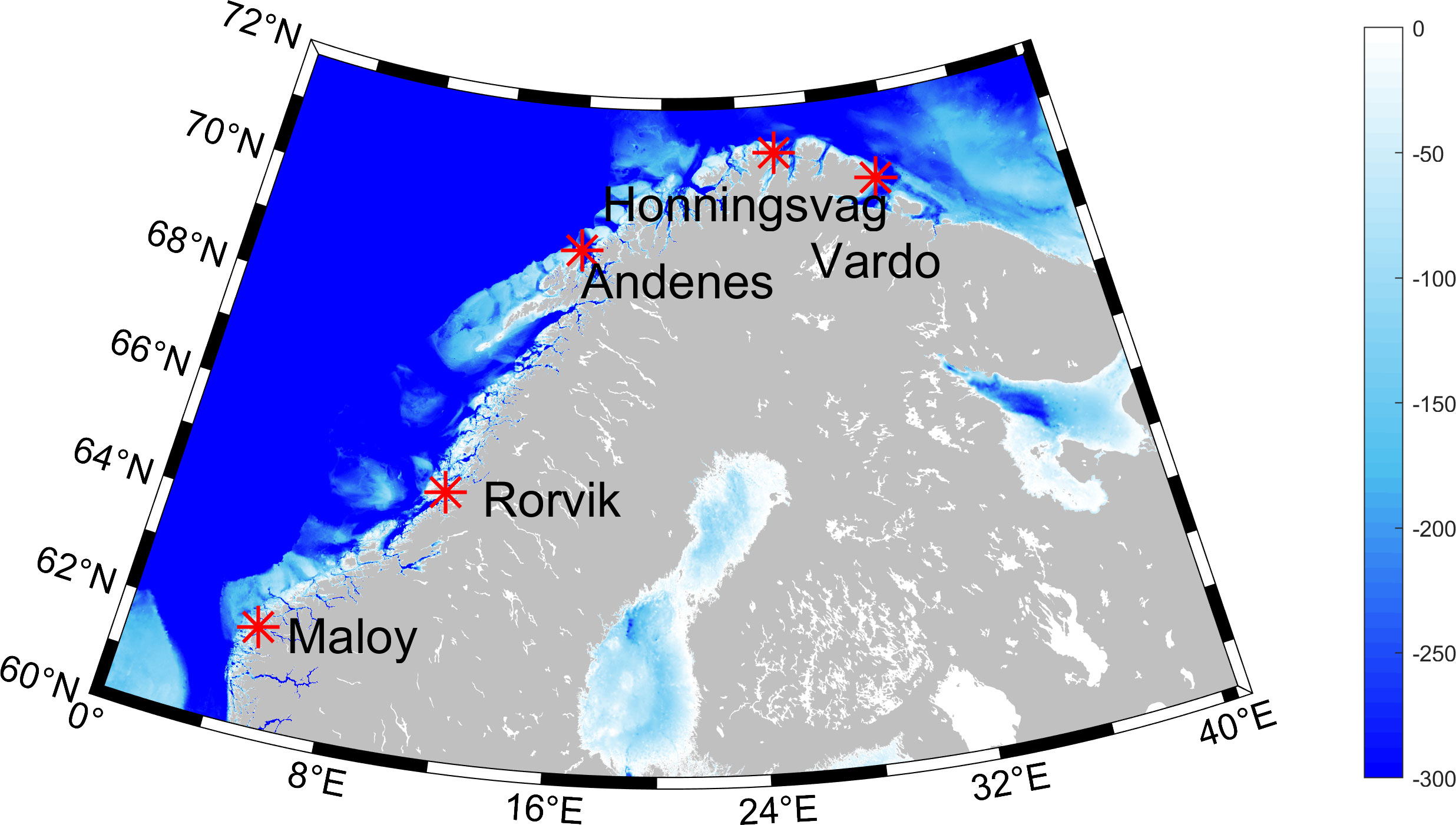
Figure 1 Bathymetry for the continental shelf in the Norwegian Sea and locations for the five tidal gauge stations.

The hourly water level records for these five gauges are sourced from the University of Hawaii Sea Level Center (https://uhslc.soest.hawaii.edu/). Additionally, Norwegian sea surface height (SSH) data is obtained from the Simple Ocean Data Assimilation (SODA) (https://climatedataguide.ucar.edu/climate-data/soda-simple-ocean-data-assimilation). The spatial resolution of this data is 0.5°x0.5°. Time records from 1980 to 2015, and timestep is monthly.

The hourly water level records are segmented into annual time frames, with each interval undergoing independent harmonic analysis using the T_TIDE toolbox (Pawlowicz et al., 2002). Throughout the data processing, any gaps in the original data are replaced with NaN values. If the missing data within a yearly time frame exceeds 25%, the corresponding window is marked as a NaN value. Therefore, a few months of data is abandoned in the five stations. More detailed information about the five gauges and their respective water level records can be found in Table 1.

Table 1

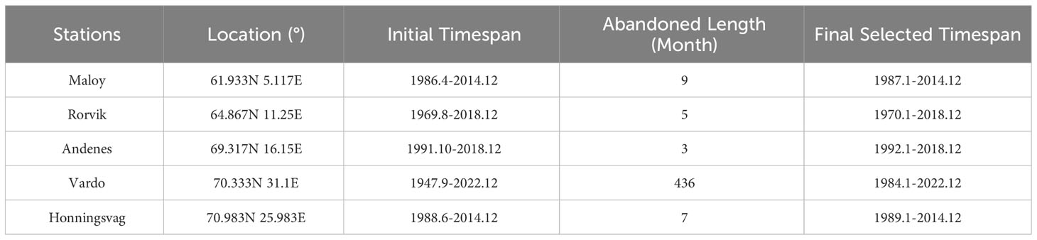
Table 1 Information for the five tide gauges.

The timespan indicates the start and end dates of the data used in the study, excluding any missing data. The “Abandoned Length (Month)” term denotes the number of months that are excluded from the initial data set due to missing data within these months. At the Vardo station, 436 months of data are excluded due to a substantial data gap before 1984. This missing data hinders the study of tidal nodal modulation. Consequently, this study chooses to analyze the data after 1984 at this station. Utilizing the T_TIDE toolbox, the amplitudes of eight tidal constituents (M₂, S₂, K₁, O₁, N₂, P₁, 2N₂, MO₃) at five stations are calculated. The averaged amplitudes of these tidal components throughout the entire study period are presented in Table 2.

Table 2

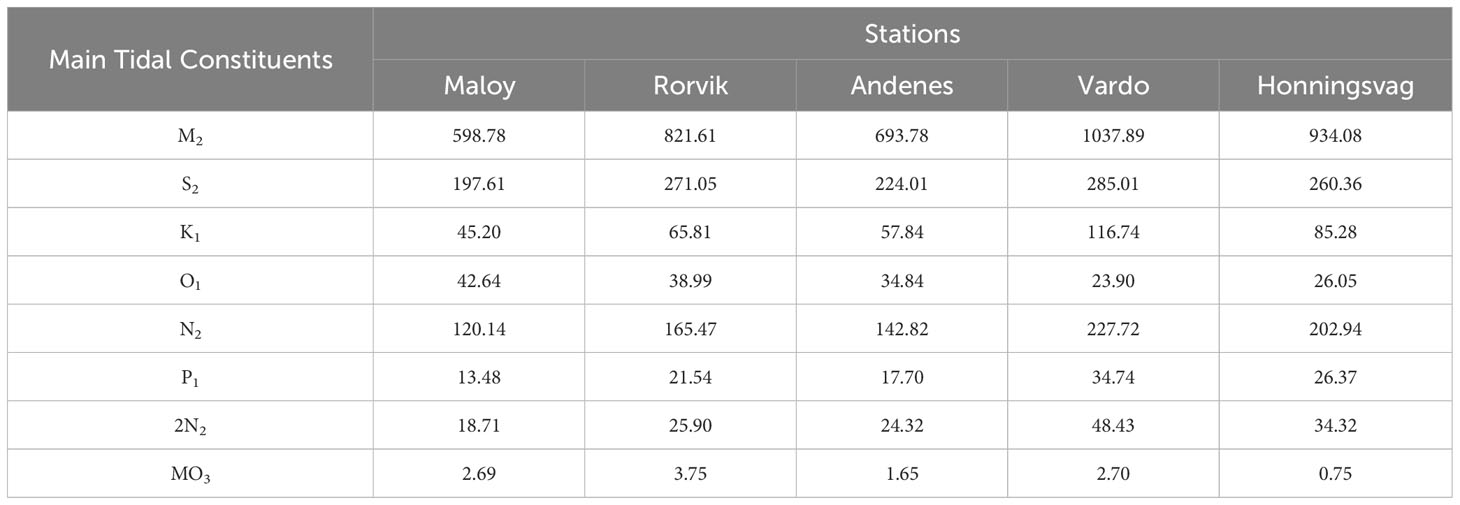
Table 2 Average amplitudes (mm) of the eight main tidal constituents at five tide gauge stations.

Among the eight primary tidal constituents, their amplitudes vary across different stations, with the maximum amplitude recorded at the Vardo station and the minimum at the Honningsvag station. The main tidal constituents observed at all five tidal stations are M₂, S₂, and N₂, and the M₂ tide constitutes the largest proportion.

2.2 Methods

The conventional harmonic and extreme analysis always obscure the 18.61-, 8.85-, and 4.42-year cycles and dedicated techniques are required for their identification (Eliot, 2010). The EHA method is proposed to investigate the temporal variations in internal tides (Jin et al., 2018). Here, we use it to analyze tidal variations in the 18.61-, 8.85-, and 4.42-year cycles along the Norwegian coast.

Traditionally, based on the least-squares method, the amplitude or phase for a tidal constituent can be estimated by:

$\begin{array}{ll}P(t)=A_0+A_{1}t+a\cos \left(\frac{2\pi }{c_0}t\right)+b\sin \left(\frac{2\pi }{c_0}t\right),& (1)\end{array}$

where P(t) represents the tidal amplitude or phase corresponding to a specific moment in time, A₀ is a constant, and A₁ represents the linear trend. c₀ indicates the period value, which is measured in years. a and b represent amplitudes of the cosine and sine functions of the cycle. Based on the fitting Equation (1), the amplitude and phase of the cycle can be expressed as:

$\begin{array}{ll}\begin{array}{l}H=\sqrt{a^2+b^2}\\ G=\arctan (b/a).\end{array}& (2)\end{array}$

The EHA method considers the amplitude and phase to be time-varying under the influence of these cycles. Thus, the amplitudes and phases of each tidal component can be obtained:

$\begin{array}{ll}P(t)=A_0+A_{1}t+a_{c_0}(t)\cos \left(\frac{2\pi }{c_0}t\right)+b_{c_0}(t)\sin \left(\frac{2\pi }{c_0}t\right),& (3)\end{array}$

and the temporal amplitude and phase:

$\begin{array}{ll}\begin{array}{l}{H}_{c0}(t)=\sqrt{{a_{c0}(t)}^2+{b_{c0}(t)}^2}\\ G_{c0}(t)=\arctan (b_{c0}(t)/a_{c0}(t)),\end{array}& (4)\end{array}$

where a_c0(t) and b_c0(t) represent the temporal amplitudes of the cosine and sine functions corresponding to the cycle c₀. H_c0(t) and G_c0(t) are the time-varying amplitude and phase corresponding to the cycle c₀. The amplitude and phase determined by Equation (2) are constant, whereas they are temporally varying as calculated by Equation (4).

Equation (3) is solved using an independent point scheme. In plain terms, the independent point scheme selects certain points within the time cycle, called independent points (IPs), and interpolates for the complete time cycle using values on IPs (See Equation (5)). We choose the value of the i-th IP as the independent parameters (denoted as a_c0,_i, b_c0,_i), and the values of other points can be obtained through interpolation between IPs. Therefore, a_c0(t) and b_c0(t) can be represented as:

$\begin{array}{ll}\begin{array}{l}{a}_{c_0}(t)={\displaystyle {\sum }_{i=1}^m{w}_{co,t,i}}\times a_{co,i}\\ b_{c_0}(t)={\displaystyle {\sum }_{i=1}^m{w}_{co,t,i}}\times b_{co,i},\end{array}& (5)\end{array}$

where m represents the number of IPs, and w_c0, _t, _i represents the weighted coefficient of the i-th independent point at time t corresponding to the cycle c_o. Considering the smoothness and small error of the curve obtained by cubic spline interpolation, this method is applied to interpolation. According to the EHA method, a MATLAB toolbox named S_TIDE was developed (Pan et al., 2018). The number of IPs is an important parameter in S_TIDE. Different IP numbers represent oscillations over various time scales.

Considering the data timespans (Table 1), the analysis for the 18.61-year cycle is only conducted at the Rorvik and Vardo stations. At these two stations, we process the M₂, S₂, N₂, and 2N₂ constituents with periods of 18.61 years and 8.85 years. Preliminary data analysis indicates that the S₂ and 2N₂ tides showed low sensitivity to these cycles, while the M₂ and N₂ tides are markedly influenced by the 18.61-year cycle. Meanwhile, due to the relatively short data duration at the Andenes, Honningsvag, and Maloy stations, we focus on processing the M₂, N₂, and 2N₂ tides for 4.42-year cycle at these three stations. Preliminary results highlight noteworthy sensitivity of the 2N₂ tide to the 4.42-year cycle at these stations. This research delves into the long-term modulations associated with these three tidal constituents using the EHA method.

3 Results

3.1 The determination of IPs

A parameter must be decided before extracting time-varying lunar cycles in the S_TIDE toolbox. The parameter is the number of IPs, which profoundly affects the accuracy of results (Pan et al., 2018). Overmuch IPs can result in overfitting, while too few IPs may lead to a higher root mean square error (RMSE). Therefore, determining the appropriate IP number is important. Three criteria are employed to determine the IP number: signal-to-noise ratio (SNR), the RMSE between hindcasts obtained by the S_TIDE and the original dataset, and a 95% confidence interval.

Firstly, this study imposes constraints on the SNR. Conventional research considered an SNR greater than two to be reliable (Matte et al., 2013), but more rigorous criteria are introduced in this study. This study not only demands an SNR greater than two but also emphasizes that the SNR should ideally exhibit a declining trend. Secondly, by comparing the RMSE, the degree of result deviation from the observations can be determined. A smaller RMSE indicates superior outcomes. Thirdly, the shorter the 95% confidence interval the more accurate results. When other conditions are reasonably met, evaluating the length of the 95% confidence interval facilitates a more informed selection. By consideration of the SNR requirement, a comprehensive assessment of RMSE and the 95% confidence interval allows for the optimal determination of IPs.

As an example, we present a detailed procedure for determining the number of IPs for the 4.42-year cycle of the 2N₂ tide at the Andenes station. Table 3 provides the SNR, RMSE, and 95% confidence interval with different numbers of IPs.

Table 3

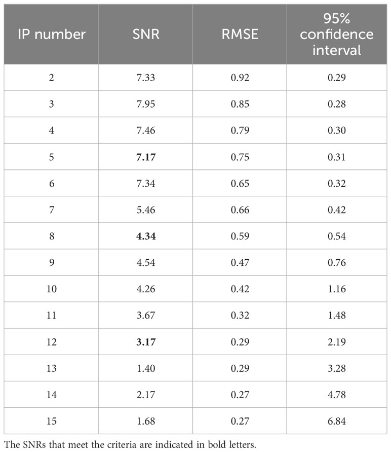
Table 3 The SNR, RMSE, and length of 95% confidence interval with different numbers of IPs at Andenes station.

The SNRs meeting the criteria correspond to the IP numbers 5, 8, and 12. Then, the RMSE and the length of the 95% confidence interval must be thoroughly evaluated. Observing Table 3, it is noted that when the number of IP is set to 8, the corresponding RMSE is smaller than that with a number 5, with a slightly longer confidence interval. When the number of IP is set to 12, the RMSE decreases again, but the length of the confidence interval markedly increases. Taking the number of IP = 2 as a benchmark, there is an 18.6% decrease in RMSE and a 7.9% increase in the confidence interval when the number is set to 5. With IP of 8, the RMSE decreases by 35.9%, and the confidence interval length expands by 86.9%. When the number of 12 is employed, the RMSE diminishes by 67.9%, but the confidence interval length increases by 653.4%, and overfitting appears. Thus, the number of IPs set to 5 is the optimal choice overall. Using the same methodology and following the same steps, the optimal number of IPs for the 18.61-year cycle of M₂ and N₂ tides, and the 4.42-year cycle of 2N₂ tide at five stations are determined, and they are listed in Table 4.

Table 4

Table 4 The optimal numbers of IPs for the 18.61-year cycle of M₂ and N₂ tides, and the 4.42-year cycle of 2N₂ tide at five stations.

Using the best-fit IPs, the S_TIDE toolbox generates hindcast amplitudes for M₂, N₂, and 2N₂ tides. These hindcast values are then compared with observations to validate the chosen of IPs number. The results show a strong agreement between the hindcast amplitudes and observations (Figures 2, 3), barring a few extreme values possibly influenced by weather conditions or tidal resonance (Talke and Jay, 2020). This indicates that the optimal IPs identified through the aforementioned methodology are reasonable and appropriate.

Figure 2

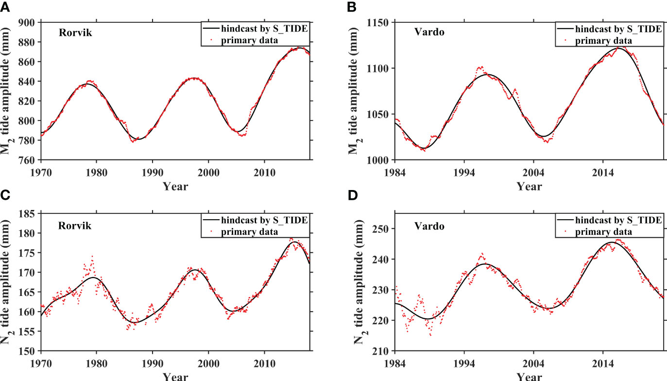
Figure 2 The primary amplitudes (red dots) and the hindcasts amplitudes by the S_TIDE (black lines) of M₂ (A, B) and N₂ (C, D) tides at Rorvik and Vardo stations with optimal IPs for the 18.61-year cycle.

Figure 3

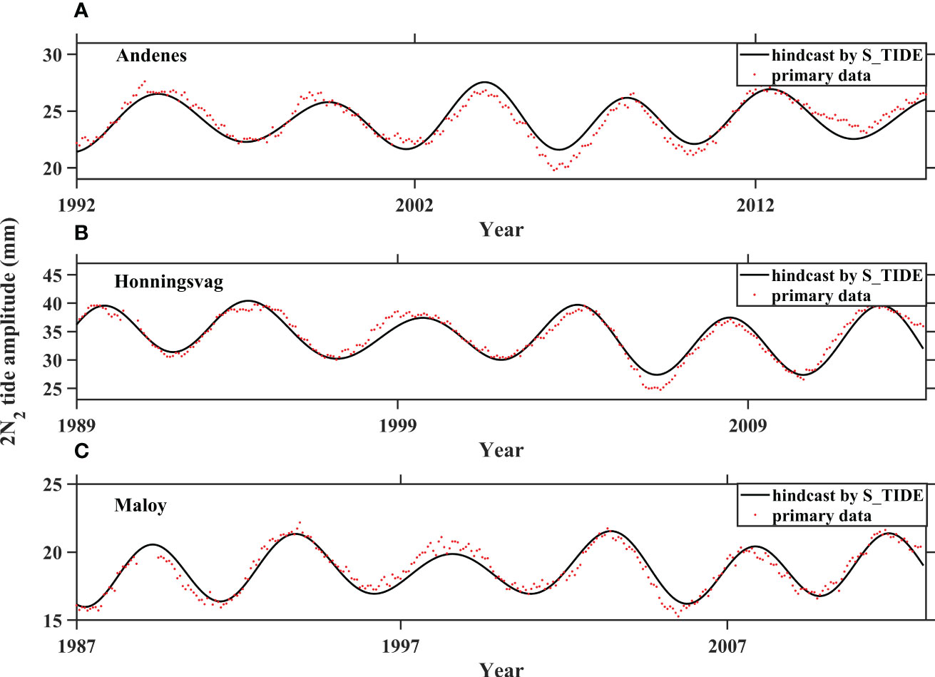
Figure 3 The primary amplitudes (red dots) and the hindcasts amplitudes by the S_TIDE (black lines) of 2N₂ at Andenes (A), Honningsvag (B), and Maloy stations (C) with optimal IPs for the 4.42-year cycle.

3.2 18.61-year cycle and 4.42-year cycle

Using the optimal number of IPs, the S_TIDE toolbox extracts time-varying cycles for the M₂, N₂, and 2N₂ tides at the five stations, as shown in Figure 4. Spatial variations in the fluctuations caused by these cycles are observed among the stations. For the 18.61-year cycle, the effects are more pronounced at the Rorvik station for the M₂ tide (Figure 4A) and the opposite for N₂ tide at both stations (Figure 4B). The nodal amplitudes of M₂ and N₂ exhibit a similar variation trend, initially increasing, then decreasing, and finally increasing again. As a whole, the trends of these two tides are increasing with different rates at both stations. The M₂ shows a larger rate at the Rorvik station, while the N₂ has a larger rate at the Vardo station.

Figure 4

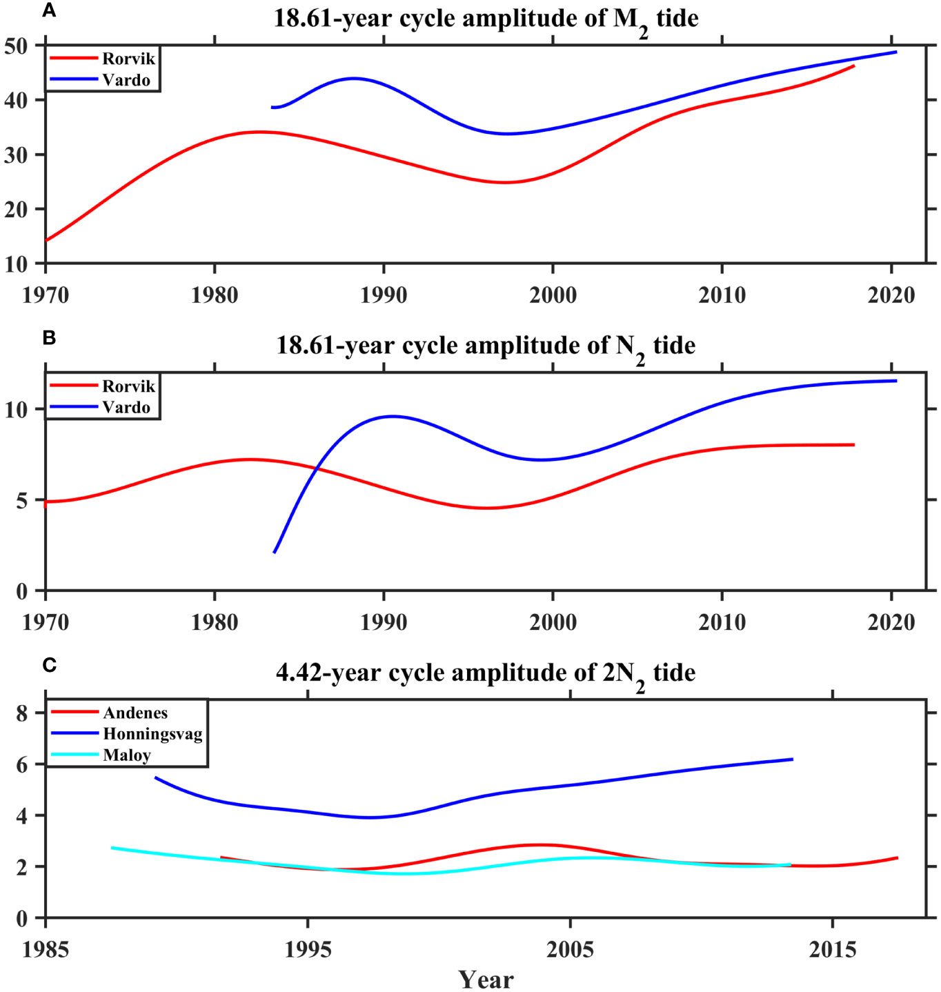
Figure 4 The 18.61-year cycle amplitudes (mm) of M₂ tide (A) and N₂ tide (B) at Rorvik and Vardo, and 4.42-year cycle amplitudes (mm) of 2N₂ tide at Andenes, Honningsvag, and Maloy (C).

During the study period, the variation amplitude reaches up to 32 mm for the M₂ tide at the Rorvik station and 9.5 mm for the N₂ tide at Vardo stations. The traditional viewpoint of the M₂ nodal cycle’s amplitude being 3.73% of the tidal amplitude (Müller, 2011) is challenged, as the ratio ranges between 1.72% to 5.63% at Rorvik station and 3.25% to 4.70% at Vardo station. This suggests that nodal amplitude has prominent spatial and temporal variations, and considering it as a constant is insufficient, highlighting the importance of nodal modulation in evaluating long-term water level trends.

Compared to the amplitudes of nodal cycle, the 4.42-year cycle exhibits slight variations in amplitudes. The maximum amplitudes of the 4.42-year cycle are observed at the Honningsvag station, while they are minimal at the Maloy station. This aligns with the mean amplitudes of 2N₂ tide at the three stations (shown in Table 2). For the 2N₂ tide, the amplitudes of the 4.42-year cycle show an increasing linear trend at the Honningsvag station, while they are very slightly decreasing at the other two stations.

Figure 5 displays the 95% confidence intervals for the 18.61-year cycle of the M₂ and N₂ tides at the Rorvik and Vardo stations, and Figure 6 presents intervals for the 4.42-year cycle of the 2N₂ tide at the Andenes, Honningsvag, and Maloy stations. These intervals are relatively small and all of them exhibit temporal modulations, confirming the effectiveness of the EHA method in extracting temporal amplitudes for those long-term cycles.

Figure 5

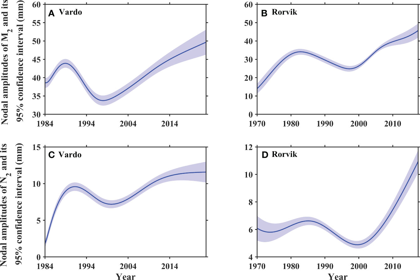
Figure 5 Nodal amplitudes and their 95% confidence intervals of M₂ (A, B) and N₂ (C, D) tides at the Vardo and Rorvik stations. The shading represents the 95% confidence interval.

Figure 6

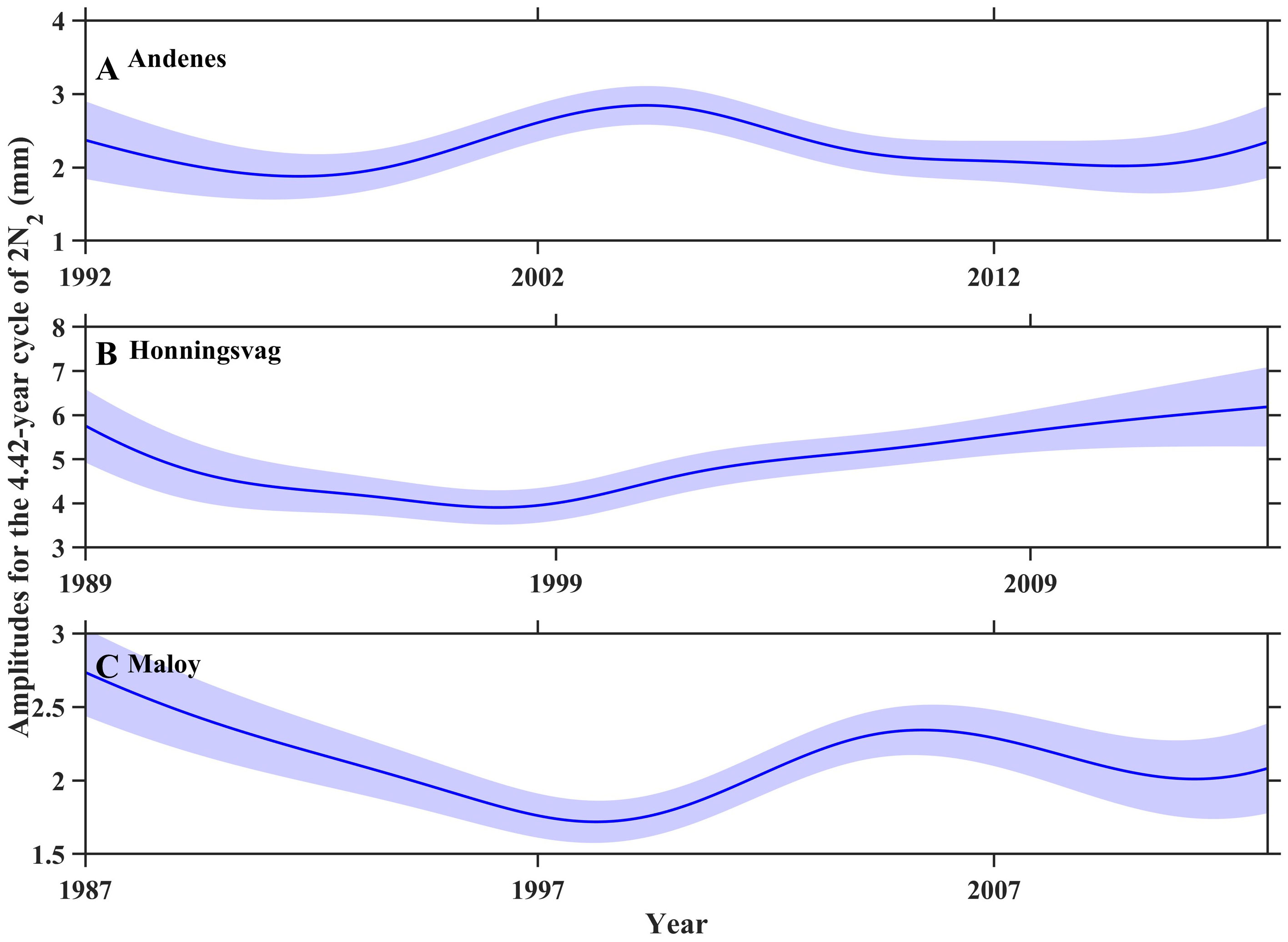
Figure 6 Amplitudes for the 4.42-year cycle of 2N₂ tide and their 95% confidence intervals at the Andenes (A), Honningsvag (B), and Maloy stations (C). The shading represents the 95% confidence interval.

4 Discussion

4.1 The time series of sea levels

As illustrated in Figure 4, the nodal amplitudes of M₂ and N₂, along with the 4.42-year cycle’s amplitude of 2N₂, display noticeable spatial and temporal variations across these stations. Previous studies have indicated that the tidal variation is influenced by sea level changes (Santamaria-Aguilar et al., 2017), and high tide levels are proportional to sea level rise (Idier et al., 2017). In Figure 7, the time series of sea levels and their linear trends are presented. These sea levels exhibit intricate temporal fluctuations, with all showing an increasing linear trend except for the Honningsvag station. The increasing trends of nodal amplitudes of M₂ and N₂ correspond to the linear trends of sea levels at the two stations. However, they are opposite for the trends of the 4.42-year cycle’s amplitude of 2N₂ with the linear trends of sea levels at the other three stations. The increasing trend of the 4.42-year cycle’s amplitude corresponds to the decreasing linear trend of sea levels at the Honningsvag station. Conversely, the decreasing trends of the 4.42-year cycle’s amplitude correspond to the increasing linear trend of sea levels at the Andenes and Maloy stations. This suggests that the lunar cycles are influenced by sea levels, while being sensitive to the specific tidal constituent and local topography.

Figure 7

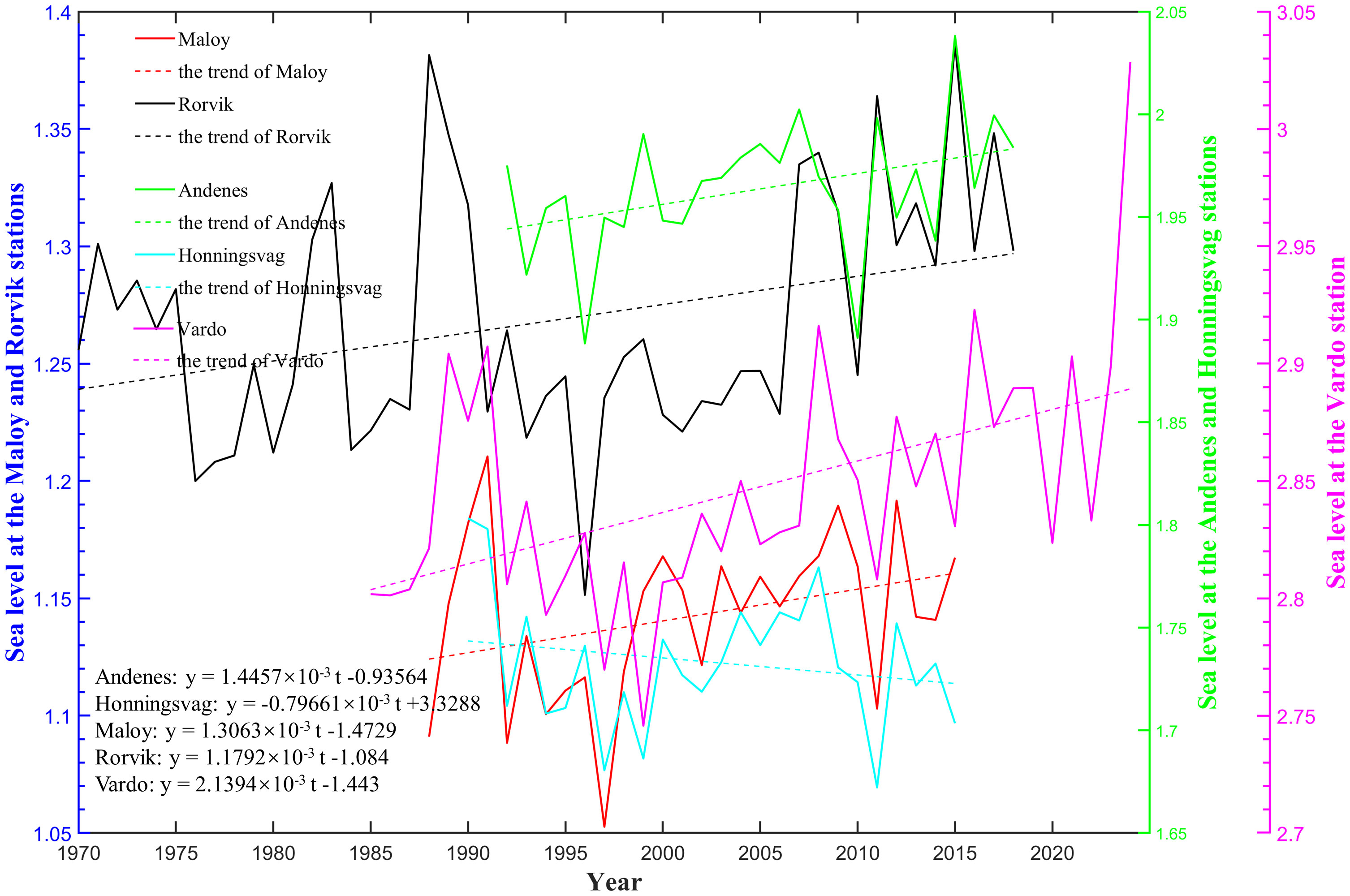
Figure 7 Year-averaged time series of sea levels and its trends at the five gauge stations (m). Please note that the sea levels and their trends at the Maloy and Rorvik stations are represented on the blue axis, while those at Andenes and Honningsvag stations are on the green axis.

4.2 Topography

The transition between ocean tides and the continental shelf and coastline occurs through resonance, which is influenced by the shape of the coast and the depth of the coastal waters (Woodworth et al., 2019). Irregularities in the seafloor terrain cause tidal waves to scatter and refract during propagation, thereby influencing the distribution of tidal amplitudes. In shallow coastal regions, the coastline forms intricate shapes, potentially leading to crucial impacts on sea level variations (Woodworth et al., 2019). Sea level fluctuations across different stations are closely connected to local topography.

When comparing the tidal amplitudes listed in Table 2, it is evident that the Vardo station has the largest amplitudes for the three primary tidal constituents (M₂, S₂, N₂), while the Maloy station has the smallest. This trend appears to follow the longitudes of the stations, with one exception at the Rorvik station where the amplitudes for the three main tidal constituents are larger compared to the Andenes station, even surpassing the S₂ amplitude at the Honningsvag station. This difference may be due to the topography (Woodworth et al., 2019). The Andenes station faces the open ocean, while the Rorvik station is located in a narrow strait (Figure 8). It is important to note that the response of tidal amplitudes to seafloor terrain and coastline varies depending on the tidal constituents. For example, the O₁ amplitudes show an opposite trend in variation compared to the M₂ amplitudes among the five stations. Therefore, the tidal amplitudes are influenced by both the seafloor terrain in the offshore and the coastline, and the responses of tides are specific to certain tidal constituents.

Figure 8

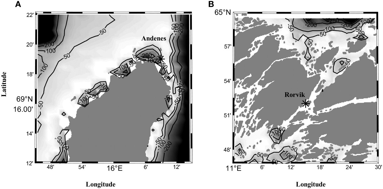
Figure 8 Topography around the Andenes (A) and Rorvik (B) stations.

4.3 Mesoscale activity

Using the SODA data, Figure 9A illustrates the climatic distribution of SSH above the geoid. The SSH exhibits prominent variations, with denser isolines in offshore water, indicating heightened large circulation and mesoscale activities. Monthly SSH anomaly is calculated from 1980 to 2015, and they almost all show prevalent mesoscale activities, giving the SSH anomaly in May 1992 as an example (Figure 9B). A previous study identified interconnected eddies in the Norwegian Sea, propagating northward and generating anticyclonic eddies through compression against the coastline (Ikeda et al., 1989). Altimetry and ocean color data from the satellite were used to investigate anticyclonic eddies in the Norwegian Sea, and a coupled physical-primary production ocean model provided three-dimensional information on the structure and properties of these eddies (Hansen et al., 2010). These active mesoscale eddies play a vital role in sea level variations, even contributing to extreme sea-level events (Firing and Merrifield, 2004). Therefore, the impact of mesoscale activity on sea level fluctuations deserves careful consideration.

Figure 9

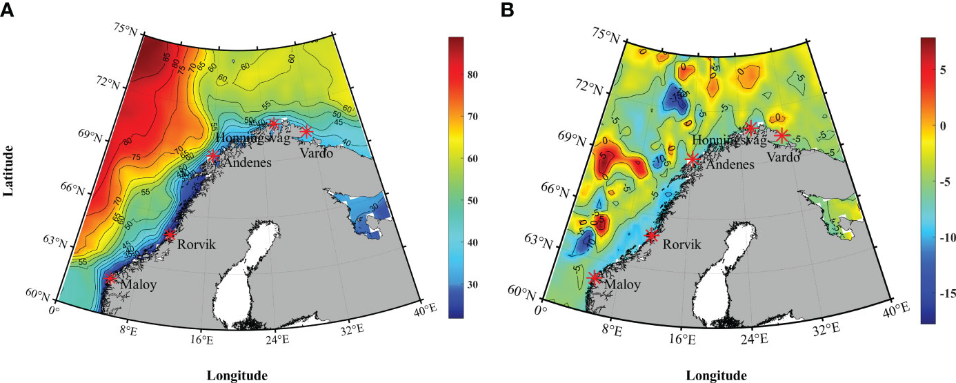
Figure 9 (A) Climatic distribution of SSH (cm) in the Norwegian Sea, (B) SSH anomaly (cm) in the Norwegian Sea in May 1992.

The spatial- and 10 days-averaged SSH anomaly time series data, from July 12, 2010, to December 21, 2021, and its trend are shown in Figure 10, sourced from the Aviso (https://tds.aviso.altimetry.fr/). It reveals complex temporal fluctuations, with the SSH anomaly increasing at a rate of 6.5 mm/year over the entire time series, indicating an enhanced trend of mesoscale activity in the Norwegian Sea. Essentially, this indicates that mesoscale activities persist consistently, and their intensity is on the rise in the Norwegian Sea. These active and robust mesoscale activities conspicuously impact sea level variations and can even lead to extreme sea-level events (Firing and Merrifield, 2004), thereby altering the tides and lunar cycles of tides.

Figure 10

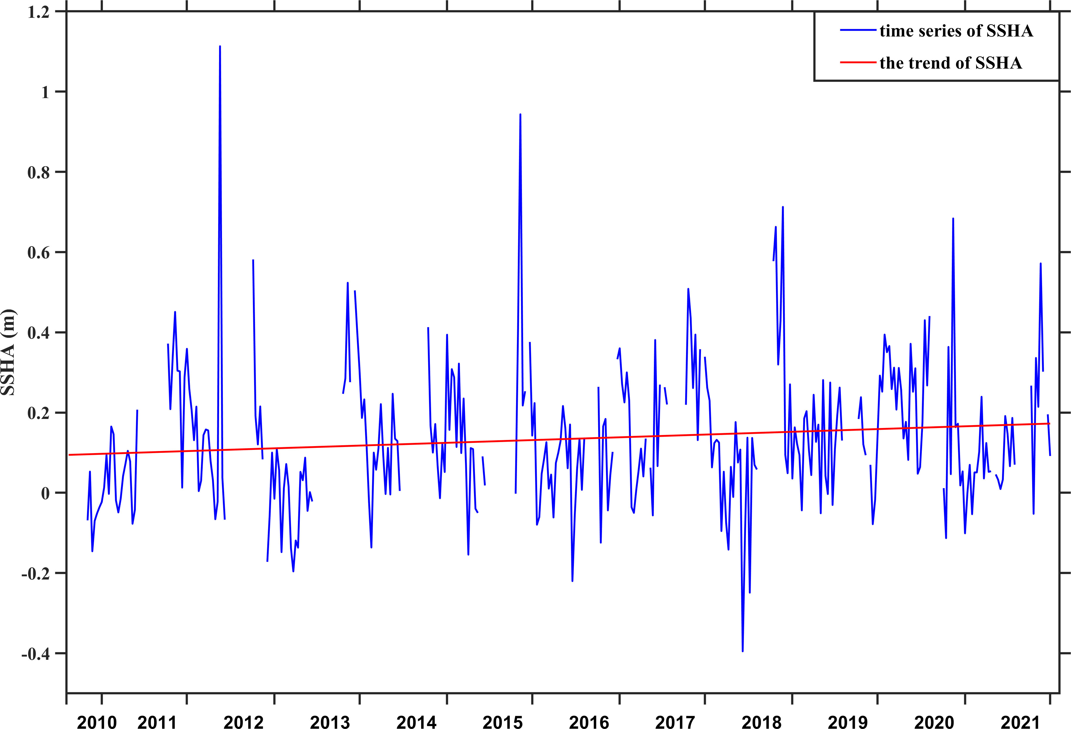
Figure 10 Time series of spatial- and 10 days-averaged SSH anomalies in the study region (blue line, 0-40°E, 60-75°N) and its trend (red line).

5 Conclusions

In this study, five tidal gauge stations (Maloy, Rorvik, Andenes, Vardo, and Honningsvag) have been chosen to investigate the nodal modulation of M₂ and N₂ tides along the Norwegian coast. Unlike the traditional tidal harmonic analysis method, the EHA method considers the amplitudes and phases of nodal cycles as temporally variable. Nodal modulation has been proven to markedly impact sea levels, particularly in high-latitude coastal regions in the face of global warming (Peng et al., 2019). This paper implements the S_TIDE toolbox, developed from the EHA method, to obtain the temporal nodal amplitudes and confirms its effectiveness by comparing hindcast results with primary data.

The tidal gauge station data are decomposed into eight tidal constituents using T_TIDE toolbox, and three tides, M₂, N₂, and 2N₂, are selected through the preliminary data processing. Due to the length of the primary data, the 18.61-year cycle of M₂ and N₂ tides is explored at Rorvik and Vardo stations, while the 4.42-year cycle of 2N₂ tide is analyzed at other three stations. The amplitudes of 18.61-year cycle of M₂ and N₂ exhibit an increasing trend, aligning with the trends of sea levels at the Rorvik and Vardo stations. The amplitudes of 4.42-year cycle of 2N₂ show an increasing trend at the Honningsvag station, while they are decreasing at the other two stations. These trends are opposite with trends of sea levels at the three stations. The amplitudes of the two cycles show noticeable spatial and temporal variations among the five stations, which can be attributed to the changes of sea levels, local topography, and the active and robust mesoscale activities.

The ratio of the M₂ nodal cycle’s amplitude to the M₂ mean amplitude ranges from 1.72% to 5.63% at Rorvik station and from 3.25% to 4.70% at Vardo station. This shows that treating the nodal cycle’s amplitude as a constant is inadequate. Nodal modulation exhibits temporal and spatial variations, which must be taken into account when evaluating tidal variations over interdecadal periods.

Data availability statement

The original contributions presented in the study are included in the article/supplementary material. Further inquiries can be directed to the corresponding author.

Author contributions

XZ: Conceptualization, Formal analysis, Methodology, Writing – original draft, Writing – review & editing. JZ: Conceptualization, Formal analysis, Methodology, Writing – original draft, Writing – review & editing. MY: Data curation, Writing – original draft. SZ: Supervision, Writing – review & editing. FD: Validation, Writing – review & editing. QL: Validation, Writing – review & editing. WZ: Validation, Writing – review & editing. ZC: Resources, Software, Supervision, Writing – review & editing.

Funding

The author(s) declare financial support was received for the research, authorship, and/or publication of this article. This study is supported by the National Natural Science Foundation of China (Grants 42206028, 42276013, 92158201, and 42106028), the Guangdong Basic and Applied Basic Research Foundation (2021A1515110171), the Innovation and Entrepreneurship Project of Shantou (Grant 201112176541391), the Independent Research Project Program of State Key Laboratory of Tropical Oceanography (LTOZZ2201), and the National Key R&D Program of China (2022YFE0203500).

Acknowledgments

We are grateful to Haidong Pan for providing the S_TIDE toolbox.

Conflict of interest

The authors declare that the research was conducted in the absence of any commercial or financial relationships that could be construed as a potential conflict of interest.

Publisher’s note

All claims expressed in this article are solely those of the authors and do not necessarily represent those of their affiliated organizations, or those of the publisher, the editors and the reviewers. Any product that may be evaluated in this article, or claim that may be made by its manufacturer, is not guaranteed or endorsed by the publisher.

References

Bij de Vaate I., Vasulkar A. N., Slobbe D. C., Verlaan M. (2021). The influence of Arctic landfast ice on seasonal modulation of the M₂ tide. J. Geophysical Res.: Oceans 126, e2020JC016630. doi: 10.1029/2020JC016630

CrossRef Full Text | Google Scholar

Devlin A. T., Jay D. A., Talke S. A., Zaron E. D., Pan J., Lin H. (2017). Coupling of sea level and tidal range changes, with implications for future water levels. Sci. Rep. 7, 17021. doi: 10.1038/s41598-017-17056-z

PubMed Abstract | CrossRef Full Text | Google Scholar

Eliot M. (2010). Influence of interannual tidal modulation on coastal flooding along the Western Australian coast. J. Geophysical Res.: Oceans 115, 1. doi: 10.1029/2010JC006306

CrossRef Full Text | Google Scholar

Ezer T., Haigh I. D., Woodworth P. L. (2016). Nonlinear sea-level trends and long-term variability on western European coasts. J. Coast. Res. 32, 744–755. doi: 10.2112/JCOASTRES-D-15-00165.1

CrossRef Full Text | Google Scholar

Feng X., Tsimplis M. N., Woodworth P. L. (2015). Nodal variations and long-term changes in the main tides on the coasts of China. J. Geophysical Res.: Oceans 120, 1215–1232. doi: 10.1002/2014JC010312

CrossRef Full Text | Google Scholar

Firing Y. L., Merrifield M. A. (2004). Extreme sea level events at Hawaii: Influence of mesoscale eddies. Geophysical Res. Lett. 31, 1–4. doi: 10.1029/2004GL021539

CrossRef Full Text | Google Scholar

Frederikse T., Riva R., Kleinherenbrink M., Wada Y., van den Broeke M., Marzeion B. (2016). Closing the sea level budget on a regional scale: Trends and variability on the Northwestern European continental shelf. Geophysical Res. Lett. 43, 10–864. doi: 10.1002/2016GL070750

CrossRef Full Text | Google Scholar

Hagen R., Plüß A., Jänicke L., Freund J., Jensen J., Kösters F. (2021). A combined modeling and measurement approach to assess the nodal tide modulation in the North Sea. J. Geophysical Res.: Oceans 126, e2020JC016364. doi: 10.1029/2020JC016364

CrossRef Full Text | Google Scholar

Hansen C., Kvaleberg E., Samuelsen A. (2010). Anticyclonic eddies in the Norwegian Sea; their generation, evolution and impact on primary production. Deep Sea Res. Part I: Oceanographic Res. Papers 57, 1079–1091. doi: 10.1016/j.dsr.2010.05.013

CrossRef Full Text | Google Scholar

Henry O., Prandi P., Llovel W., Cazenave A., Jevrejeva S., Stammer D., et al. (2012). Tide gauge-based sea level variations since 1950 along the Norwegian and Russian coasts of the Arctic Ocean: Contribution of the steric and mass components. J. Geophysical Res.: Oceans 117, 8–10. doi: 10.1029/2011JC007706

CrossRef Full Text | Google Scholar

Idier D., Paris F., Le Cozannet G., Boulahya F., Dumas F. (2017). Sea-level rise impacts on the tides of the European Shelf. Continental Shelf Res. 137, 56–71. doi: 10.1016/j.csr.2017.01.007

CrossRef Full Text | Google Scholar

Idžanović M., Gerlach C., Breili K., Andersen O. B. (2019). An attempt to observe vertical land motion along the Norwegian coast by CryoSat-2 and tide gauges. Remote Sensing 11, 744. doi: 10.3390/rs11070744

CrossRef Full Text | Google Scholar

Ikeda M., Johannessen J. A., Lygre K., Sandven S. (1989). A process study of mesoscale meanders and eddies in the Norwegian Coastal Current. J. Phys. Oceanography 19, 20–35.

Google Scholar

Jin G., Pan H., Zhang Q., Lv X., Zhao W., Gao Y. (2018). Determination of harmonic parameters with temporal variations: An enhanced harmonic analysis algorithm and application to internal tidal currents in the South China Sea. J. Atmospheric Oceanic Technol 35, 1375–1398. doi: 10.1175/JTECH-D-16-0239.1

CrossRef Full Text | Google Scholar

Kerr R. A. (2007). Global warming is changing the world. Science 316, 188–190. doi: 10.1126/science.316.5822.188

PubMed Abstract | CrossRef Full Text | Google Scholar

Kleptsova O., Pietrzak J. D. (2018). High resolution tidal model of Canadian Arctic Archipelago, Baffin and Hudson Bay. Ocean Modelling 128, 15–47. doi: 10.1016/j.ocemod.2018.06.001

CrossRef Full Text | Google Scholar

Kristensen N. M., Røed L. P., Sætra Ø. (2023). A forecasting and warning system of storm surge events along the Norwegian coast. Environ. Fluid Mechanics 23, 307–329. doi: 10.1007/s10652-022-09871-4

CrossRef Full Text | Google Scholar

Kulikov M. E., Medvedev I. P., Kondrin A. T. (2018). Seasonal variability of tides in the Arctic Seas. Russian J. Earth Sci. 18, 1–14. doi: 10.2205/2018ES000633

CrossRef Full Text | Google Scholar

Kumar A., Yadav J., Mohan R. (2020). Global warming leading to alarming recession of the Arctic sea-ice cover: Insights from remote sensing observations and model reanalysis. Heliyon 6, 2–10. doi: 10.1016/j.heliyon.2020.e04355

CrossRef Full Text | Google Scholar

Lu H., Hu Y., Wang C., Liu W., Ma G., Han Q., et al. (2019). Effects of high temperature and drought stress on the expression of gene encoding enzymes and the activity of key enzymes involved in starch biosynthesis in wheat grains. Front. Plant Sci. 10. doi: 10.3389/fpls.2019.01414

CrossRef Full Text | Google Scholar

Luneva M. V., Aksenov Y., Harle J. D., Holt J. T. (2015). The effects of tides on the water mass mixing and sea ice in the Arctic Ocean. J. Geophysical Res.: Oceans 120, 6669–6699. doi: 10.1002/2014JC010310

CrossRef Full Text | Google Scholar

Mangini F., Chafik L., Bonaduce A., Bertino L., Nilsen J.E.Ø. (2022). Sea-level variability and change along the Norwegian coast between 2003 and 2018 from satellite altimetry, tide gauges, and hydrography. Ocean Sci. 18, 331–359. doi: 10.5194/os-18-331-2022

CrossRef Full Text | Google Scholar

Matte P., Jay D. A., Zaron E. D. (2013). Adaptation of classical tidal harmonic analysis to nonstationary tides, with application to river tides. J. Atmospheric Oceanic Technol. 30, 569–589. doi: 10.1175/JTECH-D-12-00016.1

CrossRef Full Text | Google Scholar

Milly P. C. D., Wetherald R. T., Dunne K. A., Delworth T. L. (2002). Increasing risk of great floods in a changing climate. Nature 415, 514–517. doi: 10.1038/415514a

PubMed Abstract | CrossRef Full Text | Google Scholar

Müller M. (2011). Rapid change in semi-diurnal tides in the North Atlantic since 1980. Geophysical Res. Lett. 38, L11602. doi: 10.1029/2011GL047312

CrossRef Full Text | Google Scholar

Müller M., Cherniawsky J. Y., Foreman M. G., von Storch J. S. (2014). Seasonal variation of the M₂ tide. Ocean Dynamics 64, 159–177. doi: 10.1007/s10236-013-0679-0

CrossRef Full Text | Google Scholar

Nicholls R. J. (2004). Coastal flooding and wetland loss in the 21st century: changes under the SRES climate and socio-economic scenarios. Global Environ. Change 14, 69–86. doi: 10.1016/j.gloenvcha.2003.10.007

CrossRef Full Text | Google Scholar

Oka A., Hasumi H. (2006). Effects of model resolution on salt transport through northern high-latitude passages and Atlantic meridional overturning circulation. Ocean Modelling 13, 126–147. doi: 10.1016/j.ocemod.2005.12.004

CrossRef Full Text | Google Scholar

Pan H., Devlin A. T., Xu T., Lv X., Wei Z. (2022). Anomalous 18.61-year nodal cycles in the gulf of tonkin revealed by tide gauges and satellite altimeter records. Remote Sensing 14, 3672. doi: 10.3390/rs14153672

CrossRef Full Text | Google Scholar

Pan H., Lv X., Wang Y., Matte P., Chen H., Jin G. (2018). Exploration of tidal-fluvial interaction in the Columbia River estuary using S_TIDE. J. Geophysical Res.: Oceans 123, 6598–6619. doi: 10.1029/2018JC014146

CrossRef Full Text | Google Scholar

Pan H., Zheng Q., Lv X. (2019). Temporal changes in the response of the nodal modulation of the M₂ tide in the Gulf of Maine. Continental Shelf Res. 186, 13–20. doi: 10.1016/j.csr.2019.07.007

CrossRef Full Text | Google Scholar

Pawlowicz R., Beardsley B., Lentz S. (2002). Classical tidal harmonic analysis including error estimates in MATLAB using T_TIDE. Comput. Geosci. 28, 929–937. doi: 10.1016/S0098-3004(02)00013-4

CrossRef Full Text | Google Scholar

Peng D., Hill E. M., Meltzner A. J., Switzer A. D. (2019). Tide gauge records show that the 18.61-year nodal tidal cycle can change high water levels by up to 30 cm. J. Geophysical Res.: Oceans 124, 736–749. doi: 10.1029/2018JC014695

CrossRef Full Text | Google Scholar

Richter K., Nilsen J.Ø., Drange H. (2012). Contributions to sea level variability along the Norwegian coast for 1960–2010. J. Geophysical Res.: Oceans 117, 5–11. doi: 10.1029/2011JC007826

CrossRef Full Text | Google Scholar

Santamaria-Aguilar S., Schuerch M., Vafeidis A. T., Carretero S. C. (2017). Long-term trends and variability of water levels and tides in Buenos Aires and Mar del Plata, Argentina. Front. Mar. Sci. 4. doi: 10.3389/fmars.2017.00380

CrossRef Full Text | Google Scholar

St-Laurent P., Saucier F. J., Dumais J. F. (2008). On the modification of tides in a seasonally ice-covered sea. J. Geophysical Res.: Oceans 113, 4–9. doi: 10.1029/2007JC004614

CrossRef Full Text | Google Scholar

Talke S. A., Jay D. A. (2020). Changing tides: The role of natural and anthropogenic factors. Annu. Rev. Mar. Sci. 12, 121–151. doi: 10.1146/annurev-marine-010419-010727

CrossRef Full Text | Google Scholar

Woodworth P. L., Melet A., Marcos M., Ray R. D., Wöppelmann G., Sasaki Y. N., et al. (2019). Forcing factors affecting sea level changes at the coast. Surveys Geophysics 40, 1351–1397. doi: 10.1007/s10712-019-09531-1

CrossRef Full Text | Google Scholar

Zong X., Zhang R., Zhang S., Deng F., Zhou W., Chen Z. (2021). An analysis of the 8.85-and 4.42-year cycles in the gulf of maine. J. Mar. Sci. Engineering 9, 1362. doi: 10.3390/jmse9121362

CrossRef Full Text | Google Scholar