Numerical simulation of hydrodynamics of ocean-observation-used remotely operated vehicle

1 Introduction

The underwater robots offer a significant role in maritime engineering equipment. In addition to having a more flexible operating mode and the ability to be outfitted with various operating instruments for a variety of activities and working settings, underwater robots also provide a number of benefits over other types of equipment in terms of operational efficiency. Additionally, using underwater robots, which can function at depths that divers are unable to reach, may speed up human progress into the deep sea. In addition to being able to function in unique settings that divers are unable to access, underwater robots are also often used in nuclear waste cleaning operations in nuclear power plant reservoirs. This efficiently preserves practitioner safety and enhances nuclear power plant safety. Underwater vehicles have been classified into many categories, including autonomous underwater vehicles (AUVs), remotely operated vehicles (ROVs), and underwater gliders (UGs). Among them, ROVs are divided into three types: self-propelled in water, towed, and crawling (Dalibor and Marcin, 2024). AUVs are not bound by cables, have a large range of activities, and have good concealment performance, but their underwater operation time is affected by the amount of energy they carry. The energy of the ROV is provided by the mother ship through cables, and it is capable of carrying out complex underwater operations for a long time, and is currently the most widely used underwater robot (Zhang et al., 2023).

The United States created the first ROV in 1960 and called it “CURV1”. First shown to the public at large, this ROV type was instrumental in retrieving a hydrogen bomb that had been abandoned by the US in Spanish seas (Whitcomb and Yoerger, 1993; Fan et al., 2012; Cepeda et al., 2023). During this time, ROVs were just starting out; the primary function of these early ROVs was to assist the military with recovery operations. Owing to the effects of the Middle East oil crisis in the 1970s, nations all over the globe dedicated significant resources to the study and creation of machinery for the extraction of subterranean oil. The offshore oil sector is expanding, and with it, so is the need for ROVs to monitor offshore oil platforms. The major working waters of this kind of ROV are in the North Sea oilfield, and its birth also signals the market acknowledgment of the ROV business and builds a firm market basis for the long-term growth of the ROV industry (Christophe, 2023; Selig et al., 2023).

The performance of ROVs has significantly improved between the early 1980s of the 20^th century and the early 21^st century. The most notable improvements have been in the operating depth, operating range, and operating duration of ROVs, which have been developed by various nations. The development of large-scale “operational-grade” ROVs at this time was mainly driven by the exploration of seabed resources by different nations, which improved human knowledge of the kinds and composition of resources in the deep sea and on the seabed. As a result of this era’s progress, ROVs are now in the large-scale manufacturing phase and have amassed the necessary technology to enter the large-scale commercial usage phase (Ren and Hu, 2023). Since the beginning of the 21^st century, the evolution of ROVs has been characterized by functional diversity and miniaturization. The future development trend for ROVs is miniaturization and intelligence, which will drive industry upgrading and further development of ROVs in aquaculture, military reconnaissance, underwater equipment maintenance, and marine resource development.

In order to save design expenses and increase efficiency, it is crucial to accurately determine the ROV’s hydrodynamic coefficients. These coefficients are then used to make selections about the ROV’s layout, propeller model, and handling performance. At present, the following methods are typically used to determine the hydrodynamic coefficient of underwater vehicles: system identification, experimentation with constraint models, empirical formula technique, and CFD software simulation calculation method. The empirical formula is the empirical or semi-empirical formula produced by synthesizing the data acquired by a vast number of previous model experiments or ROV actual excursion. By considering the analysis of control systems that are designed to maximize the operability limits for launch and recovery of a ROV from a small unmanned surface vessel (USV), Ahsan Tanveer and Sarvat Mushtaq Ahmad (Tanveer and Ahmad, 2023) use numerical simulation for the analysis, where the method combines recent approaches for wave compensating dynamic positioning, active heave compensation, and positioning control of the ROV with multi-body dynamic simulation of the surface vessel and ROV, including hydrodynamic forces and dynamic interactions from wires that depend on the ROV depth and moonpool. A fuzzy adaptive controller considering thruster dynamics is proposed by Mingjie et al. to improve the trajectory tracking performance of work-class ROVs (Mingjie et al., 2023). The system identification approach involves using the ROV’s motion data from real navigation or the experimental data from the constraint model to build a mathematical model. This model is then used to estimate the hydrodynamic coefficients that describe the ROV’s hydrodynamic performance.

The rapid advancement and widespread adoption of high-speed computers in recent years have allowed several scientific researchers to notice that computational fluid dynamics (CFD) software can rapidly calculate the hydrodynamic force of ROV. The previous approaches’ drawbacks may be successfully addressed by the CFD software simulation technique, which can also assist researchers in increasing the effectiveness of their R&D and confirming if the hydrodynamic performance of ROV satisfies design specifications. SKORPA (Skorpa, 2012) performed hydrodynamic numerical simulation calculations on the WR-200 ROV model by simplifying it and using CFD software to analyze the results. The findings indicate that the pitch torque of the ROV can be effectively decreased by adjusting whether the water flow passes through the middle of the ROV. Chin and Lau (2012) carried out hydrodynamic numerical computations on the ROV model using ANSYS-CFX software. The findings demonstrated that the hydrodynamic coefficients acquired by CFD software may successfully help designers enhance the structural design of ROVs.

With the wide application of underwater robots in the development of marine resources, people have more stringent requirements for the performance of underwater robots. The hydrodynamic performance of the ROV is the basis of underwater positioning, path planning and maneuvering control, and the quality of the hydrodynamic performance directly determines the success of an ROV design (Manimaran, 2022). Due to the complex shape and structure of the ROV, the ROV is affected by various complex forces such as thrust of the propulsion mechanism, water flow resistance, buoyancy, gravity and tensile force in the water, so the calculation of the hydrodynamic force of the ROV is a complex kinematic and dynamic problem. Understanding the hydrodynamic performance of ROVs is essential for several reasons. Firstly, it ensures efficient and precise operation of the vehicle, allowing operators to navigate through challenging underwater environments with accuracy. This is especially important when performing delicate tasks such as manipulating equipment, collecting samples, or conducting repairs. Furthermore, studying ROV hydrodynamic performance helps in enhancing safety. By understanding how the vehicle responds to different conditions, operators can mitigate potential risks and avoid collisions with underwater obstacles or hazards. This not only protects the ROV but also minimizes the potential damage to the surrounding environment. Moreover, the hydrodynamic performance of ROVs directly affects the speed and efficiency of tasks. By optimizing the vehicle’s maneuverability, operators can reduce the time required to complete missions, saving resources and improving overall productivity.

The motion of the ROV is a spatial motion with six degrees of freedom. According to the movement force and moment, the maneuverability mathematical model can be constructed to determine the optimal control rule and control system (Zhao et al., 2022; Zhao et al., 2023). Hydrodynamic coefficients are the coefficients of ROV motion equation. In order to simulate the motion and predict the performance of a ROV, the hydrodynamic coefficients must be determined first. The existing hydrodynamic computation techniques for ROV mainly include the following methods: system identification, experimental constraint model method, empirical formula method, and CFD simulation calculation method. However, the hydrodynamic calculation theory of AUV is more mature than that of ROV, and the hydrodynamic calculation of ROV requires further improvement and verification of the dependability of the simulation calculation technique. Thus, the hydrodynamic forces of the ROV model during straight-line and planar motion mechanism (PMM) need to be primarily determined. The purpose of this study is to show the approach and method to obtain these hydrodynamic coefficients using CFD method, and to investigate the hydrodynamic characteristics of the ROV during turning maneuver. The rest of the paper is organized as follows. Section 2 presented the mathematical models for hydrodynamics and maneuverability of ROV. Section 3 carried out a verification study of hydrodynamic numerical methods. Section 4 and 5 simulated the hydrodynamic performance of ROV in steady and unsteady motions and fitted a large number of hydrodynamic coefficients. Finally, the conclusion draw from this paper are presented in Section 6.

2 Computational theory

2.1 Mathematical models

A motion coordinate system consisting of two right-hand coordinate systems $E-\xi \eta \zeta$ and $O-xyz$ was established, as shown in Figure 1.

Figure 1

Figure 1 ROV system coordinate system.

The linear velocity and angular velocity of the ROV in the moving coordinate system can be expressed as $V_1={[V_1 V_2]}^T$, linear velocity $V_1$ is expressed as $V_1={[u v w]}^T$, angular velocity $V_2$, expressed as $V_2={[p q r]}^T$. The forces and moments experienced by the ROV in the dynamic coordinate system can be expressed as $A={[FM]}^T$, ROV is expressed as the force $F={[X Y Z]}^T$, the moment exerted is expressed as: $M={[K M N]}^T$. The force and velocity of the ROV are positive in the direction of the coordinate axis of the dynamic coordinate system, and the moment and angular velocity are determined by the right-hand rule. Table 1 shows the six ROV degrees of freedom, while Table 2 shows the motion parameters and coordinate components.

Table 1

Table 1 The six degrees of freedom of ROV.

Table 2

Table 2 Motion parameters and coordinate components.

The dynamic equation of the ROV must be established before analyzing its motion. The following assumptions are applied to the ROV model to answer the equation of motion: the ROV is a rigid body with a constant form, mass, and centroid. The hydrodynamic force of ROV is considered independent of the impact of the seabed environment and umbilical cable. The theory proposes that the center of gravity coincides with the origin of the secondary coordinate system, and the three axes of the follower coordinate system represent the inertial main axes of the ROV. The dynamic model of the ROV could be developed using the moment of inertia and the rigid body motion hypothesis, as shown in Equation (1).

$\begin{array}{ll}{M}_{RB}\dot{V}+C_{RB}(V)V=F& (1)\end{array}$

In Equation (1), $M_{RB}$ is ROV quality matrix; $C_{RB}$ is centripetal force and coriolis matrix of ROV, $C_{RB}(V)=-C_{RB}{}^T(V)$ coefficient is related to the speed of movement, whereas; F displays overall torque in the ROV. The mass-matrix of the ROV is given in Equation (2).

$\begin{array}{ll}{M}_{RB}=\left[\begin{array}{cc}m{I}_{3\times 3}& 0_{3\times 3}\\ 0_{3\times 3}& I_g\end{array}\right]& (2)\end{array}$

Herein, m is mass; I_g is inertial matrix; $I_g=diag[\begin{array}{ccc}{I}_x& I_y& I_z\end{array}]$ in I_x, I_y, I_z, as shown in Equations (3–5):

$\begin{array}{ll}{I}_x={\int }_{\nabla }\rho (y_i{}^2+z_i{}^2)d{x}_{i}d{y}_{i}d{z}_i& (3)\end{array}$

$\begin{array}{ll}{I}_y={\int }_{\nabla }\rho (z_i{}^2+x_i{}^2)d{x}_{i}d{y}_{i}d{z}_i& (4)\end{array}$

$\begin{array}{ll}{I}_z={\int }_{\nabla }\rho (x_i{}^2+y_i{}^2)d{x}_{i}d{y}_{i}d{z}_i& (5)\end{array}$

Coriolis and centripetal matrices of $C_{RB}(V)$ are depicted in Equation (6).

$\begin{array}{ll}{C}_{RB}(V)=\left[\begin{array}{cc}mS(V_2)& 0_{3\times 3}\\ 0_{3\times 3}& -S(I_g{V}_2)\end{array}\right]& (6)\end{array}$

where S is the vector multiplication operator, which can be represented by the following matrix.

$\begin{array}{ll}S(\lambda )=-S^T(\lambda )\left[\begin{array}{ccc}0& -{\lambda }_3& {\lambda }_2\\ {\lambda }_3& 0& -{\lambda }_1\\ -{\lambda }_2& {\lambda }_1& 0\end{array}\right]& (7)\end{array}$

By combining Equations (2) and (6), the Equation (7) is simplified as shown in Equation (8).

$\begin{array}{ll}\{\begin{array}{c}X=m(\dot{u}-vr+wq)\\ Y=m(\dot{v}-wp+ur)\\ Z=m(\dot{w}-uq+vp)\\ K=I_x\dot{p}+(I_z-I_y)qr\\ M=I_y\dot{q}+(I_x-I_z)rp\\ N=I_z\dot{r}+(I_y-I_x)pq\end{array}& (8)\end{array}$

To improve an analysis of the dynamical features of ROVs, it is critical to develop a hydrodynamic model that serves as the foundation for forecasting their maneuverability. In order to reduce the impact of variables like size, speed, and mass, a non-factor approach was used. The following hydrodynamic coefficients are unitless, and their unitless guidelines are shown in Table 3. By using the dimensionless rule outlined in Table 3, the dimensionless model of the ROV may be derived by applying the dimensionless hydrodynamic coefficients (Zhao et al., 2022; Zhao et al., 2023), as shown in Equations (9–14).

Table 3

Table 3 Non-dimensioning rules.

$\begin{array}{ll}\begin{array}{c}{X}_D=\frac{\rho }{2}{L}^4(X_{qq}^{\text{'}}{q}^2+X_{rr}^{\text{'}}{r}^2+X_{rp}^{\text{'}}rp)+\frac{\rho }{2}{L}^3(X_{vr}^{\text{'}}vr+X_{wq}^{\text{'}}wq)+\frac{\rho }{2}{L}^2(X_{uu}^{\text{'}}{u}^2+X_{vv}^{\text{'}}{v}^2\\ +X_{ww}^{\text{'}}{w}^2)\end{array}& (9)\end{array}$

$\begin{array}{ll}\begin{array}{c}{Y}_D=\frac{\rho }{2}{L}^4(Y_{vq}^{\text{'}}vq+Y_{wq}^{\text{'}}wq+Y_{wr}^{\text{'}}wr)+\frac{\rho }{2}{L}^3(Y_{ur}^{\text{'}}ur+Y_{up}^{\text{'}}up+Y_{v\left|r\right|}^{\text{'}}\frac{v}{\left|v\right|}\left|{(v^2+w^2)}^{\frac{1}{2}}\right||r|)\\ +\frac{\rho }{2}{L}^2(Y_{uu}^{\text{'}}{u}^2+Y_{uv}^{\text{'}}uv+Y_{v\left|v\right|}^{\text{'}}v\frac{v}{\left|v\right|}\left|{(v^2+w^2)}^{\frac{1}{2}}\right|+Y_{vw}^{\text{'}}vw)\end{array}& (10)\end{array}$

$\begin{array}{ll}\begin{array}{c}{Z}_D=\frac{\rho }{2}{L}^4(Z_{pp}^{\text{'}}pp+Z_{pr}^{\text{'}}pr+Z_{rr}^{\text{'}}rr)+\frac{\rho }{2}{L}^2(Z_{wq}^{\text{'}}\frac{w}{\left|w\right|}\left|{(v^2+w^2)}^{\frac{1}{2}}\right||q|+Z_q^{\text{'}}uq)\\ +\frac{\rho }{2}{L}^2(Z_{uu}^{\text{'}}{u}^2+Z_{uw}^{\text{'}}uw+Z_{w\left|w\right|}^{\text{'}}w\left|{(v^2+w^2)}^{\frac{1}{2}}\right|+Z_{\left|w\right|}^{\text{'}}uw+Z_{ww}^{\text{'}}w\left|{(v^2+w^2)}^{\frac{1}{2}}\right|+Z_{vv}^{\text{'}}{v}^2)\\ +\frac{\rho }{2}{L}^3(Z_{vp}^{\text{'}}vp+Z_{vr}^{\text{'}}vr)\end{array}& (11)\end{array}$

$\begin{array}{ll}\begin{array}{c}{K}_D=\frac{\rho }{2}{L}^5(K_{p\left|p\right|}^{\text{'}}p\left|p\right|+K_{pq}^{\text{'}}pq+K_{pr}^{\text{'}}pr)+\frac{\rho }{2}{L}^4(K_{up}^{\text{'}}up+K_{ur}^{\text{'}}ur+K_{vp}^{\text{'}}vp+K_{wq}^{\text{'}}wq+K_{wr}^{\text{'}}wr)\\ +\frac{\rho }{2}{L}^4(K_{uu}^{\text{'}}{u}^2+K_{uv}^{\text{'}}uv+K_{v\left|v\right|}^{\text{'}}v\left|{(v^2+w^2)}^{\frac{1}{2}}\right|+K_{vw}^{\text{'}}vw)\end{array}& (12)\end{array}$

$\begin{array}{ll}\begin{array}{c}{M}_D=\frac{\rho }{2}{L}^3(M_{uw}^{\text{'}}uw+M_{uu}^{\text{'}}{u}^2+M_{w\left|w\right|}^{\text{'}}w\left|{(v^2+w^2)}^{\frac{1}{2}}\right|+M_{\left|w\right|}^{\text{'}}uw+M_{w\left|w\right|}^{\text{'}}w\left|{(v^2+w^2)}^{\frac{1}{2}}\right|)\\ +\frac{\rho }{2}{L}^5(M_{pp}^{\text{'}}{p}^2+M_{q\left|q\right|}^{\text{'}}q\left|q\right|+M_{pr}^{\text{'}}pr+M_{rr}^{\text{'}}{r}^2)+\frac{\rho }{2}{L}^4(M_{uq}^{\text{'}}uq+M_{vp}^{\text{'}}vp+M_{vr}^{\text{'}}vr\\ +M_{\left|w\right|q}^{\text{'}}\left|{(v^2+w^2)}^{\frac{1}{2}}\right|q)\end{array}& (13)\end{array}$

$\begin{array}{ll}\begin{array}{c}{N}_D=\frac{\rho }{2}{L}^4(N_{up}^{\text{'}}up+N_{ur}^{\text{'}}ur+N_{vp}^{\text{'}}vp+N_{wq}^{\text{'}}wq+N_{v\left|r\right|}^{\text{'}}\frac{v}{v}\left|{(v^2+w^2)}^{\frac{1}{2}}\right||r|)+\frac{\rho }{2}{L}^3(N_{uu}^{\text{'}}{u}^2\\ +N_{uv}^{\text{'}}uv+N_{v\left|v\right|}^{\text{'}}v\left|{(v^2+w^2)}^{\frac{1}{2}}\right|+N_{vw}^{\text{'}}vw)+\frac{\rho }{2}{L}^5(N_{r|r}^{\text{'}}r|r+N_{pq}^{\text{'}}pq+N_{qr}^{\text{'}}qr)\end{array}& (14)\end{array}$

2.2 CFD basic theory

The basic theory of the governing equation is the three conservation laws: the law of conservation of momentum, the law of conservation of mass, and the law of conservation of energy. Since the solution process in this paper does not involve energy, the law of conservation of energy is not considered in the governing equation in this paper. The basic form of the equation for the conservation of momentum is the N-S equation, which was proposed by Navier-Stokes and needs to be satisfied in general fluid systems, the N-S equation form, as shown in Equation (15).

$\begin{array}{ll}\{\begin{array}{c}\rho \frac{du}{dt}=p{g}_x-\frac{\partial p}{\partial x}+\mu (\frac{{\partial }^{2}u}{\partial x^2}+\frac{{\partial }^{2}u}{\partial x^2}+\frac{{\partial }^{2}u}{\partial x^2})\\ \rho \frac{du}{dt}=p{g}_y-\frac{\partial p}{\partial y}+\mu (\frac{{\partial }^{2}u}{\partial y^2}+\frac{{\partial }^{2}u}{\partial y^2}+\frac{{\partial }^{2}u}{\partial y^2})\\ \rho \frac{du}{dt}=p{g}_z-\frac{\partial p}{\partial z}+\mu (\frac{{\partial }^{2}u}{\partial z^2}+\frac{{\partial }^{2}u}{\partial z^2}+\frac{{\partial }^{2}u}{\partial z^2})\end{array}& (15)\end{array}$

where, ρ is water density, p is pressure and µ is kinematic viscosity coefficient.

The standard representation of mass conservation is the continuity equation, which states that the mass of matter in a given space remains constant. The change in mass within a control volume is determined by the difference between the inflow and outflow of mass from that volume. This work examines an incompressible fluid with a constant density. The continuity equation is further simplified, as seen in Equation (16).

$\begin{array}{ll}\frac{\partial u}{\partial x}+\frac{\partial v}{\partial y}+\frac{\partial w}{\partial z}=0& (16)\end{array}$

Herein, u, v, w are fluid velocity components.

The standard adopted in this article is k-ε turbulence model. At present, the RANS approach is the most frequently employed approach in engineering applications to analyze turbulence models, and it is also the method utilized in this research.

$\begin{array}{ll}\rho \frac{\partial {\overline{u}}_i}{\partial t}+\rho {\overline{u}}_l\frac{\partial {\overline{u}}_i}{\partial x_j}=\rho {\overline{f}}_l+\frac{\partial \overline{p}}{\partial x_i}+\frac{\partial }{\partial x_j}(\mu \frac{\partial {\overline{u}}_i}{\partial x_j}-\rho \overline{u_i^{\text{'}}{u}_j^{\text{'}}})& (17)\end{array}$

In Equation (17), ρ -Fluid density; $\overline{p}$ -Pressure average; µ —Dynamic viscosity; $\rho \overline{u_i^{\text{'}}{u}_j^{\text{'}}}$—Reynolds stress.

In computational fluid dynamics, the basic principle of numerical solving is to solve for each discrete node to obtain an approximation of the overall flow field. The finite volume method (FVM) is used to discretize the governing equations. The wall function approach is employed to address the flow field in proximity to the wall. The development of the overset mesh approach accelerates the resolution of intricate flow fields. Its fundamental idea involves breaking down complex flow fields into smaller, independent sub-regions, with each sub-region generating a distinct mesh. When simulating complicated motions, there is no need to renew the mesh since each sub-region’s mesh shape is fixed. Complex motions could be accomplished by specifying motions inside each sub-region’s mesh.

As shown in Figure 2, the calculation steps of overset meshes mainly include: (1) sub-region division and mesh generation, (2) determining overset boundary conditions, (3) determining the interpolation type between sub-regions, and (4) calculating the flow field. In the calculation, the first three steps need to be continuously adjusted to ensure the convergence of the flow field. The difficulty of the overset mesh technique is that as the mesh position of each sub-region changes, the position of the boundary and the position of the hole area need to be determined repeatedly.

Figure 2

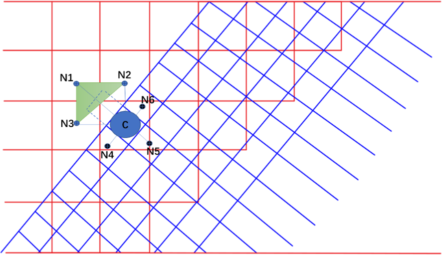
Figure 2 Overset mesh.

3 Verification of hydrodynamic numerical methods

3.1 SUBOFF Model

3.1.1 Proposal of verification methods

In order to verify the reliability of the theory proposed in this paper in the numerical calculation of underwater vehicles and the rationality of the numerical calculation model and meshing form, the standard model of underwater submersibles, the SUBOFF model, was selected for the verification of hydrodynamic numerical calculations.

3.1.2 SUBOFF Parameters of the model

The SUBOFF model has been accepted as a standard model by the ITTC. This standard model can be built according to the shape formula in ITTC. The SUBOFF model used in this paper is shown in Figure 3. The main model parameters are shown in Table 4.

Figure 3

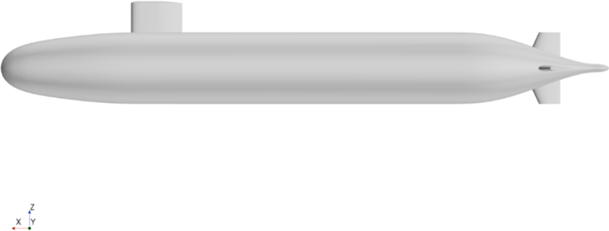
Figure 3 SUBOFF model.

Table 4

Table 4 SUBOFF model parameters.

3.2 Compute domain determination and meshing

3.2.1 Computational domain

A computational domain needs to consider whether the area is capable of ensuring fully convergent computational results and limit the percentage of invalid regions to increase computational efficiency. The size of the computational domain for this paper is calculated based on the partition of the computational domain in prior SUBOFF simulation studies. The domain length is determined by multiplying the length by 6. The height is determined by multiplying the length by 3. Similarly, the width is determined by multiplying the length by 3. Furthermore, for an adequately accelerated flow field, the submersible is situated at a distance equal to two-hull dimensions. The length of the hull from the velocity inlet is twice the length of the boat, while the length of the boat is three times the length from the pressure outlet.

3.2.2 Meshing

According to the results of the division of the calculation area, this paper divides the meshing of different regions. When meshing, the basic principle of meshing is strictly followed, and the mesh refinement is carried out in the area close to the hull, and the mesh density is reduced layer by layer in the area far away from the hull. In this paper, we select tetrahedral mesh, cut mesh, and prismatic layer mesh model, and set the basic mesh size to 0.3m, set the boundary layer to 5 layers, and set the minimum mesh size to 3.125% of the basic mesh size. Figure 4 is the longitudinal meshing result in the calculation domain, Figures 5, 6 are the meshing result of the bow and stern of the hull, respectively.

Figure 4

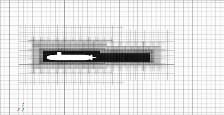
Figure 4 Vertical overall meshing results.

Figure 5

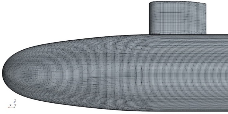
Figure 5 Bow mesh.

Figure 6

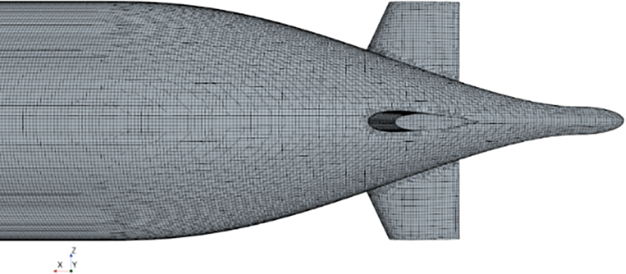
Figure 6 Stern mesh.

3.3 Simulation calculation and verification

In order to enhance computational efficiency, it is critical to reduce the proportion of invalid regions in the computational domain and ascertain whether the computational area will deliver fully convergent results when determining the computational domain. The size of the computational domain to be employed in this research is established by referring to the partition of the computational domain in the previous SUBOFF simulation studies. The width is three times the length, the height is three times the length, and the computed domain length is six times the length. Additionally, the SUBOFF is positioned at the second-hull length, the hull length is tripled from the pressure outlet, and the hull length from the velocity inlet is doubled from the hull length in order to be sure that the computed flow field has a viable acceleration area.

3.3.1 Boundary and computation conditions

The boundary conditions should be set separately in every surface of calculation domain. The boundary conditions are determined by designating the incoming flow as the velocity inlet, the outlet as the pressure outlet, the hull surface as the wall, and the surrounding surface as the wall. The standard $k-ϵ$ model is selected as the turbulence model. Five working conditions with velocities of 3.045, 5.144, 6.091, 7.161 and 8.231 m/s were selected for straight-line simulation experiments.

3.3.2 Calculation results and validity analysis

According to the boundary conditions under different working conditions, five straight-line simulations are carried out in this section, and the simulation results and the relative error results of the simulated calculation are shown in Table 5.

Table 5

Table 5 Resistance calculation value and error.

In addition, the simulation results are compared with the experimental results, as shown in Figure 7. Through the comparison curve between the experimental values and the simulated values, it can be clearly seen that the straight-line resistance value gradually increases with the increase of velocity, but the relationship between resistance and velocity is not linear. At a velocity of 3.045m/s, the error between the simulated value and the experimental value is the largest, and the reliability of the simulated value at low velocity is slightly lower than that at medium and high velocities. Overall, the simulation data are basically consistent with the experimental data, and the relative error between the two is 1%-3%, which can meet the actual standards of the project.

Figure 7

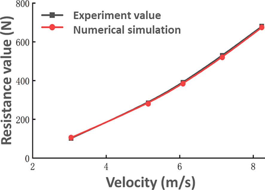
Figure 7 Comparison of simulation and experimental data.

By analyzing the SUBOFF straight-line simulation experiment, the engineering standard can be satisfied, and then it is confirmed that the calculation theory, the meshing method and the selected calculation model proposed in this paper are reasonable and reliable, so the calculation method can be popularized and used in the subsequent simulation experiments.

4 Simulation calculation of the steady motion of the ROV

4.1 ROV model simplification and computational domain division

4.1.1 Simplified ROV model

Figure 8 shows that the computational model used in this paper is based on a small ROV. In order to do simulation calculations using CFD software, it is necessary to simplify the model of the ROV by removing the complex surfaces that do not contribute to the computation. The principle of simplification encompasses several key characteristics. Firstly, the simplified model must align with the primary scale of the original model, while also preserving the essential components of the ROV. Furthermore, the internal components of the original model do not impact the simulation experiment and can be excluded. This study integrates the pertinent components of the ROV to assure the consistency of the reduced model. A basic ROV model is seen in Figure 9. The simplified model is derived by undergoing the process of simplification, and the fundamental parameters of the simplified model are shown in Table 6.

Figure 8

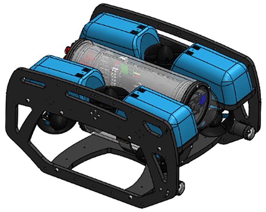
Figure 8 Three-dimensional model.

Figure 9

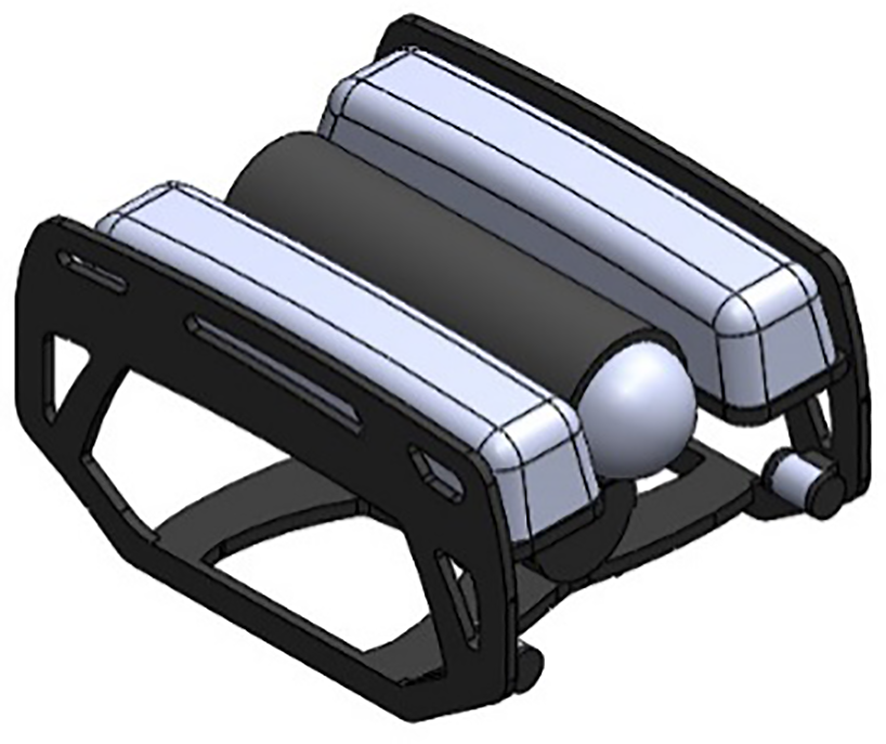
Figure 9 Simplified model.

Table 6

Table 6 ROV basic parameters.

4.1.2 Computational domain division and boundary layer setting

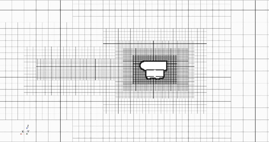
In the simulation calculation, the length of the calculated domain is 9L (L is the length of ROV), the length of the ROV from the velocity inlet is 3L, the length from the pressure outlet is 5L, the height and width of the calculated domain are taken as 5L, and the ROV is placed on the third L. In order to easily control the mesh size of different regions, it is necessary to set up an internal calculation domain in the overall calculation domain. Referring to the division of the internal computing domain of the standard model in Section 3, this paper divides the internal computing domain into two modules: hull refinement area and wake refinement area. The overall computational domain in the ROV stationary motion simulation experiment is shown in Figure 10, and the internal computational domain is shown in Figure 11.

Figure 10

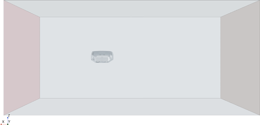
Figure 10 Overall calculation domain.

Figure 11

Figure 11 Internal computing domain.

Based on the empirical formula, the thickness of the boundary layer is 5 mm. The number of boundary layers is generally determined according to the Reynolds number of the calculated working case, and for the movement under the high Reynolds number, the number of boundary layers is set to 5-10 layers. The mesh quality under different boundary layers is compared, and the number of boundary layers is finally determined to be 5.

4.2 Mesh type and mesh independence validation

4.2.1 Mesh type

The ROV model is relatively simple in the simulation calculations to be carried out in this section; the hexahedral mesh type is used. From the tank wall to the ROV surface, the produced mesh is encrypted layer by layer, which reduces computation time and guarantees simulation calculation accuracy. Hexahedral mesh is also used in this paper’s internal calculation domain, as the ROV model does not need complicated maneuvers in the stationary motion simulation calculation.

4.2.2 Mesh independence validation

In order to ensure the accuracy and precision of the simulation results, in addition to considering the mesh type, the number of meshes is also an important influencing factor after the mesh type and calculation domain size are determined. In this paper, a mesh independence verification is designed to determine the appropriate number of meshes. Seven mesh quantities of 780,000, 1.06 million, 1.54 million, 2 million, 2.21 million, 2.53 million and 3 million were selected for independent verification, and the ROV velocity was set to 1.5m/s. The ROV forward motion simulation experiments were carried out under different mesh numbers, and the resistance values under different mesh numbers were counted, as shown in Table 7. The data in the table is generated into a resistance graph, as shown in Figure 12.

Table 7

Table 7 Different mesh resistance values.

Figure 12

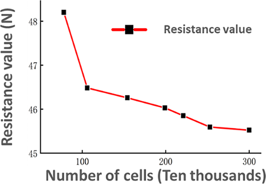
Figure 12 Resistance value changes with the number of meshes.

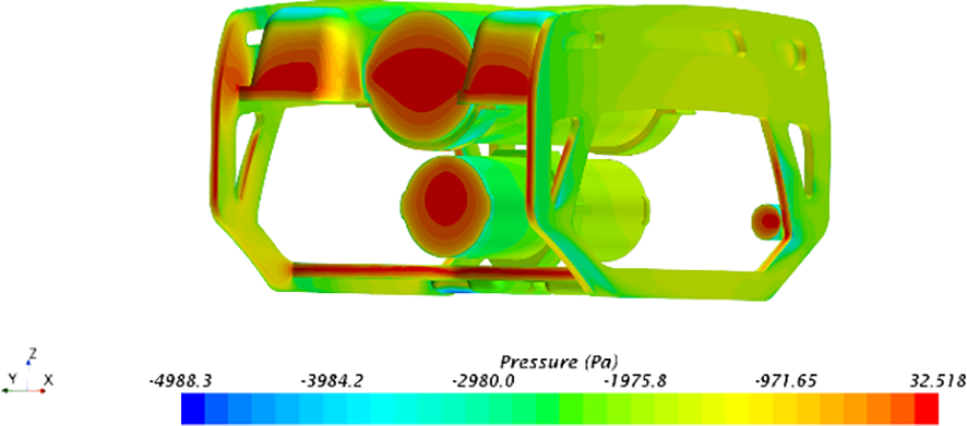
Figure 12 illustrates that the resistance value rises with a decreasing number of meshes and tends to stabilize at a certain number of meshes. Due to the large mesh size, the reproduction degree of the ROV is limited when the number of meshes is fewer than one million, which causes the ROV simulation experiment to have a high resistance value. When there are more than 2.5 million meshes, the mesh size is smaller, the ROV form is better restored, and the ROV resistance value is more in line with the experimental value. Furthermore, the resistance value tends to remain stable when the mesh count exceeds 2.5 million. This is because, beyond this threshold, further reductions in mesh size no longer enhance the reduction degree of ROV shape. Consequently, the resistance values obtained through simulation calculation under identical working conditions are congruent with the experimental values, and the resistance values remain stable. The number of meshes used in this article is 2.53 million in order to prevent having too many meshes affect the simulation computation and to take computer performance into consideration. The mesh for simulation calculations is completed based on the size of the calculation domain and the meshing form that was previously established. Figure 13 displays the longitudinal overall mesh; Figure 14 displays the head mesh of the RVO model; and Figure 15 displays the surface pressure distribution in the ROV.

Figure 13

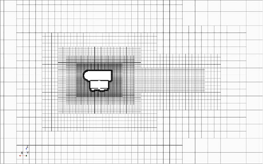
Figure 13 Longitudinal overall mesh of forward motion.

Figure 14

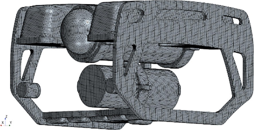
Figure 14 Header mesh.

Figure 15

Figure 15 Surface pressure distribution of forward motion.

4.3 Hydrodynamic calculations

4.3.1 Hydrodynamic calculations

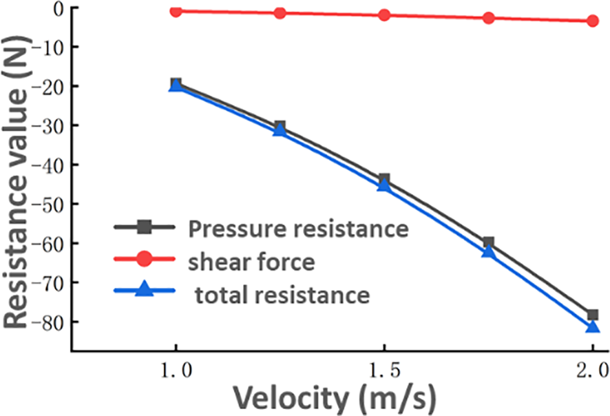
The ROV resistance under different velocities was simulated and calculated. The simulation results at different velocities are shown in Table 8. The resistance values at different velocities in Table 7 are represented by graph lines, as shown in Figures 4–9.

Table 8

Table 8 Numerical calculation results of forward motion.

Figure 16 shows that the difference between total resistance and compressive resistance grows with increasing velocity, but the values of both resistances increase linearly with increasing velocity. The fraction of pressure resistance in the overall resistance of the progressive voyage is much higher than the shear resistance. The pressure differential between the front and rear surfaces of the ROV rises as velocity increases, which also increases the pressure resistance since the compressive resistance is produced by this pressure difference between the surfaces during movement. In addition, as the velocity increases, the proportion of pressure resistance in total resistance is decreasing. Because the velocity gradient of the ROV surface flow field increases with increasing velocity, the value of the shear resistance is closely related to the velocity gradient of the flow field. In general, the increase in positive resistance is mainly due to the pressure resistance, and it is necessary to pay close attention to the shape of the front and rear surfaces of the ROV in the design of the ROV, and minimize the lateral water frontal area.

Figure 16

Figure 16 Forward resistance.

4.3.2 Hydrodynamic calculations for reverse navigation

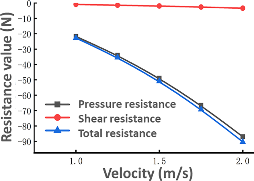
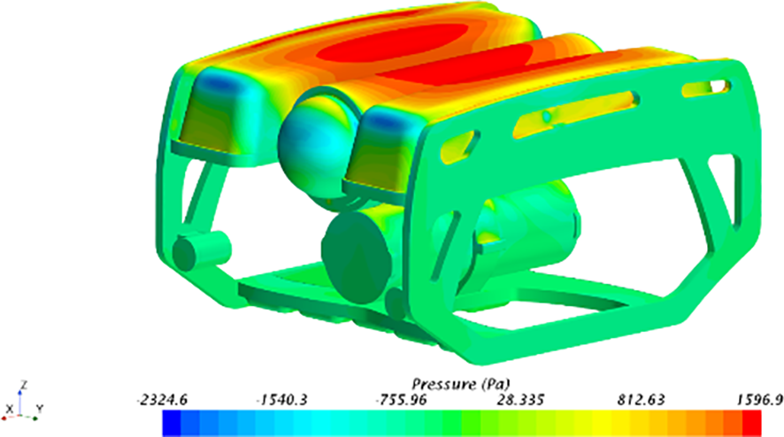
Given the asymmetrical form of the ROV in relation to the mid-cross profile, it is necessary to treat the numerical modeling of the reverse journey condition as a distinct consideration in the straight-line experiment. Similar to the actual journey, the simulation trials are conducted at five different velocities. The boundary requirements for the rear simulation are identical to those for the positive course. However, the calculation region must be partitioned again to ensure that the tail of the ROV model is oriented towards the direction of the entering flow. Figure 17 displays the longitudinal overall mesh after resetting the computation domain and mesh in the reverse navigation scenario. Figure 18 displays the distribution of surface pressure. The computed outcomes for the five operational scenarios are shown in Table 9. The information presented in the table is visually represented in the form of a graph, as seen in Figure 19.

Figure 17

Figure 17 Inverted longitudinal overall mesh.

Figure 18

Figure 18 Surface pressure distribution of reverse motion.

Table 9

Table 9 Calculation results of reverse flight value.

Figure 19

Figure 19 Inversion resistance.

The shear resistance and pressure resistance in Tables 7, 8 are plotted and compared, and the results are shown in Figures 20, 21.

Figure 20

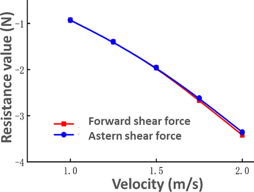
Figure 20 Shear resistance comparison.

Figure 21

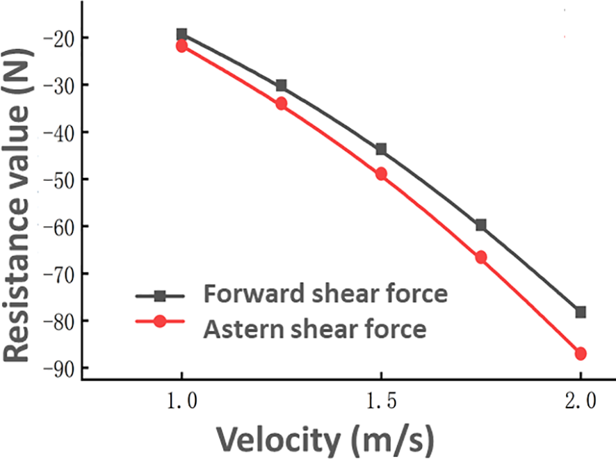
Figure 21 Comparison of pressure resistance.

In Figure 20, the shear resistances during forward and backward sailing are seen to grow as the velocity increases. Additionally, the shear resistance values for both positive and backward sailing states are almost identical at the same velocity. This is due to the similarity in velocity gradient and shear resistance along the wall of the ROV, which remains consistent at the same velocity. Figures 21, 22 clearly demonstrate a noticeable disparity in pressure resistance between the positive and backward navigation modes. Furthermore, the pressure resistance in both states escalates as the velocity rises. The compressive resistance of the ROV is influenced by its shape, particularly the asymmetry between the front and rear parts. As a result, the disturbance caused by the ROV to the surrounding flow field is different when it is moving forward compared to when it is moving in reverse. The reverse pressure resistance is greater than the positive pressure resistance at the same velocity, primarily due to the poor streamlining of the ROV tail. It can be concluded that when designing the ROV, the symmetry of the front and rear parts of the ROV should be ensured as much as possible while ensuring that the ROV shape is fluid. This shape distribution is conducive to reducing the straight-line resistance of the ROV and improving the propulsion efficiency.

Figure 22

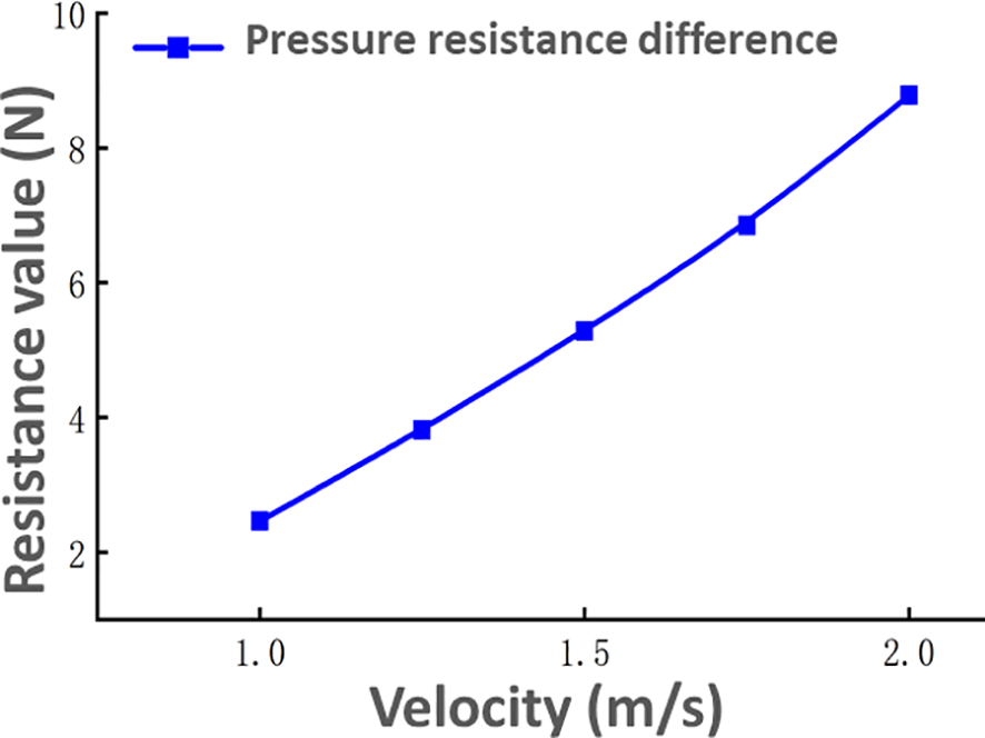
Figure 22 Differential pressure resistance.

4.3.3 Hydrodynamic calculations of ascent motion

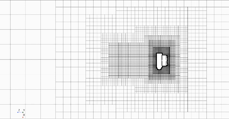
The underwater submersible is capable of executing six degrees of freedom of motion underwater. In addition to the direct motion along the x-axis, the simulation computation for stable motion should also take into account the direct motion along the y-axis and z-axis directions. This chapter focuses on simulating and calculating the direct motion of the negative direction of the z-axis. The first step involves dividing the calculation domain and creating a mesh. The meshing results for the negative direction of the z-axis are shown in Figure 23. Furthermore, the insignificance of the mesh count is confirmed, and it is established that there are precisely 2.58 million meshes without upward motion. Figure 24 displays the surface pressure distribution of the ascending motion.

Figure 23

Figure 23 Vertical overall mesh of ascending motion.

Figure 24

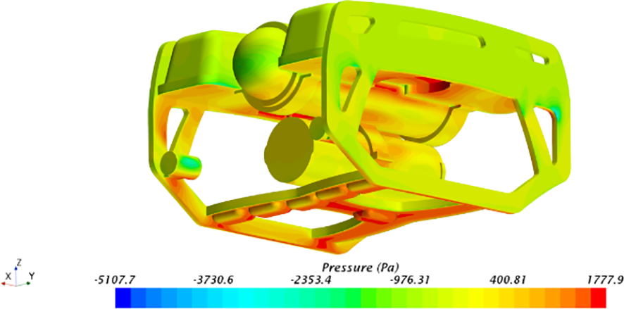
Figure 24 Pressure distribution on the surface of ascending motion.

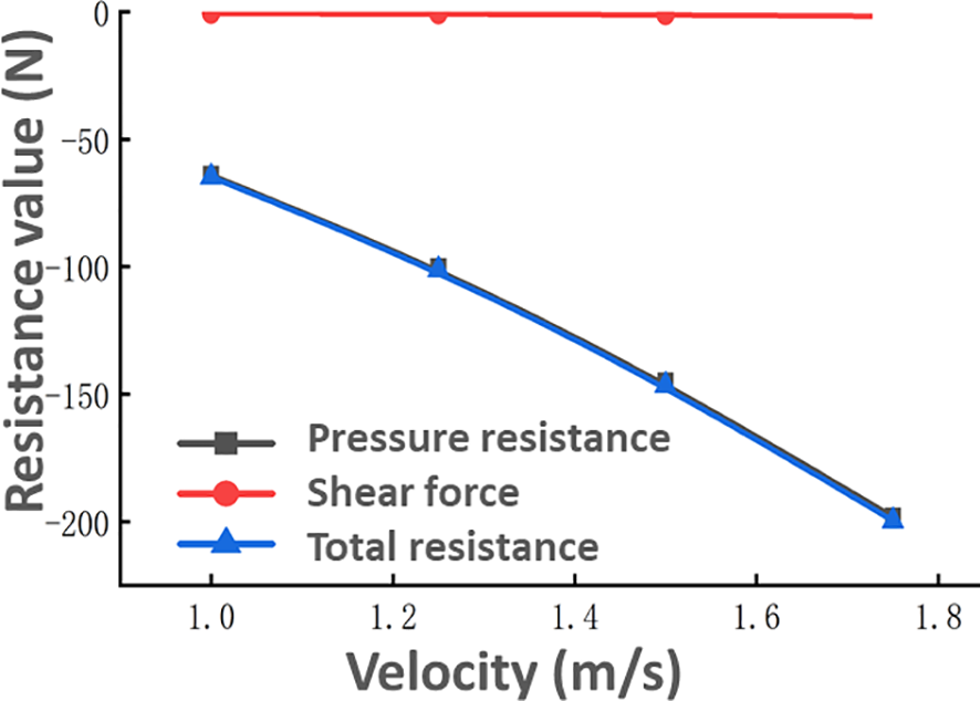
After setting the boundary conditions of the calculation model, four working conditions were selected for simulation calculation, and the simulation results are shown in Table 10.

Table 10

Table 10 Numerical calculation results of ascending movement.

The data in Table 9 are plotted as graphs, as shown in Figure 24.

Figure 25 demonstrates that the pressure resistance and shear resistance both escalate as the velocity of upward motion increases. During the upward motion, the ratio of pressure resistance to total resistance is higher compared to the motion along the x-axis, and the shear resistance is much reduced. Since the shape of the ROV is cuboidal, the waterfront area in the z-axis direction is larger than the waterfront area in the x-axis direction, the proportion of the pressure resistance caused by the pressure difference between the upper and lower surfaces in the z-axis direction in the total resistance is much greater than the ratio of the pressure resistance in the x-axis direction to the total resistance. When designing the ROV, it is necessary to comprehensively consider the ratio of the z-axis waterfront area to the x-axis waterfront area according to the working conditions of the ROV, which can effectively improve the hydrodynamic performance of the ROV.

Figure 25

Figure 25 Ascending motion resistance.

4.3.4 Hydrodynamic calculations of sinking movements

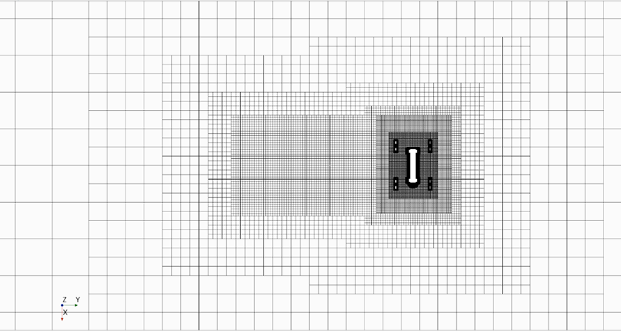
The asymmetry of the top and lower sections of the ROV is contemplated, comparable to the simulation along the x-axis. This study presents a numerical calculation of motion along the axis in both positive and negative directions. Initially, the computational domain undergoes re-meshing, and the outcome of the meshing process is shown in Figure 26. Figure 27 displays the surface pressure distribution of the descending motion.

Figure 26

Figure 26 Vertical overall mesh of sinking motion.

Figure 27

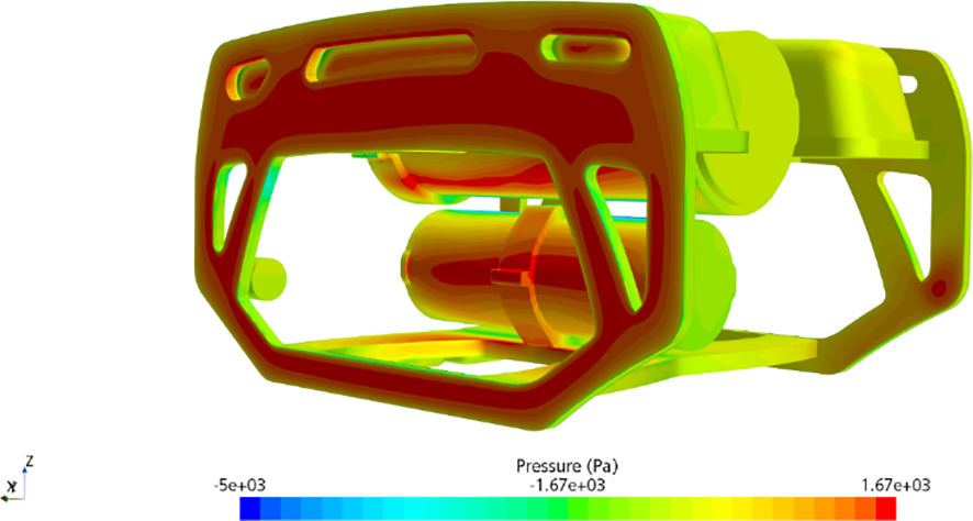
Figure 27 Surface pressure distribution of sinking motion.

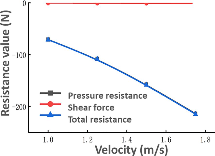
After the boundary conditions of the calculation model are set, the simulation of the four working conditions is carried out, and the simulation results are shown in Table 11.

Table 11

Table 11 Numerical calculation results of sinking motion.

The data in Table 10 are plotted as shown in Figure 28. Comparing the data in Tables 9, 10, Figures 29–31 is obtained.

Figure 28

Figure 28 Sinking resistance.

Figure 29

Figure 29 Shear resistance comparison.

Figure 30

Figure 30 Comparison of pressure resistance.

Figure 31

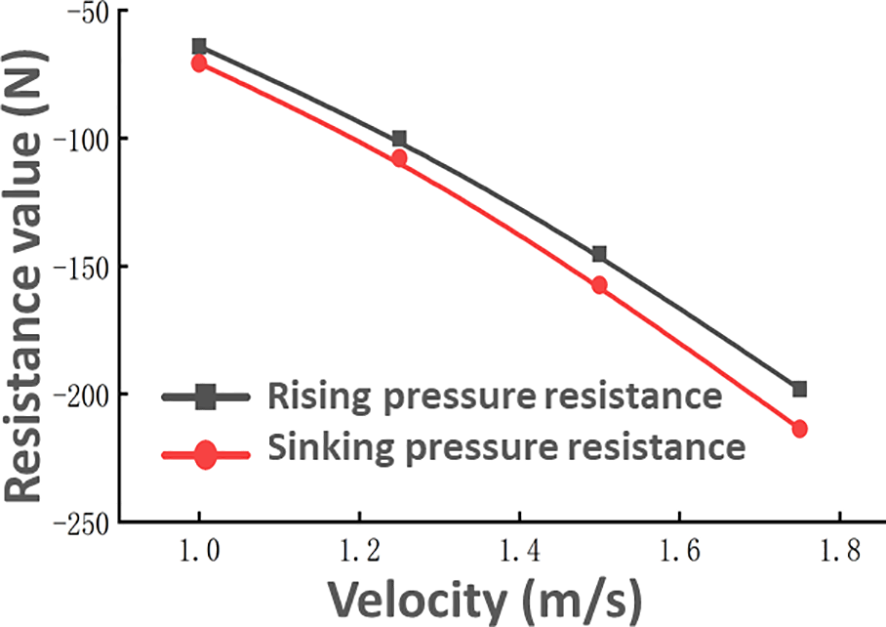
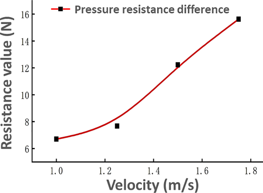
Figure 31 Pressure resistance difference.

By analyzing the data in Figures 29–31, it is assessed that in the ascending and sinking motions, the resistance of the ascending motion is less than that of the sinking motion. Different from the experimental data of forward and reverse sailing, the shear resistance and pressure resistance in the ascending and descending motion have obvious changes at the same velocity. The change of shear resistance relative to the pressure resistance is small, and the pressure resistance accounts for a large proportion of the difference between the two states. In this regard, the causes of the upward and downward movements are analyzed in depth, and due to the asymmetry of the upper and lower parts of the ROV shape, the pressure difference between the upper and lower surfaces in the upward and downward movements is different, which makes the difference in the downward pressure resistance of the two working conditions. In addition, because the water facing area in the z-axis heave motion is greater than the forward navigation motion of the x-axis, the motion of the z-axis has a great influence on the flow field around the ROV, and the velocity gradient near the wall of the ROV changes significantly in the ascending and sinking motions, which leads to the difference between the shear resistances of the two motion states.

4.3.5 Hydrodynamic calculations for lateral movements

Considering that the left and right parts of the ROV are symmetrical, only one direction is selected for numerical calculation of the movement along the y-axis. The meshing and computational domains were re-meshed, and the meshing results are shown in Figure 32. The surface pressure distribution is shown in Figure 33.

Figure 32

Figure 32 Vertical overall mesh of lateral motion.

Figure 33

Figure 33 Pressure distribution on surface of lateral motion.

The simulation results of the four calculation cases are shown in Table 12.

Table 12

Table 12 Numerical calculation results of lateral movement.

The graph is plotted based on the data in Table 11, as shown in Figure 34.

Figure 34

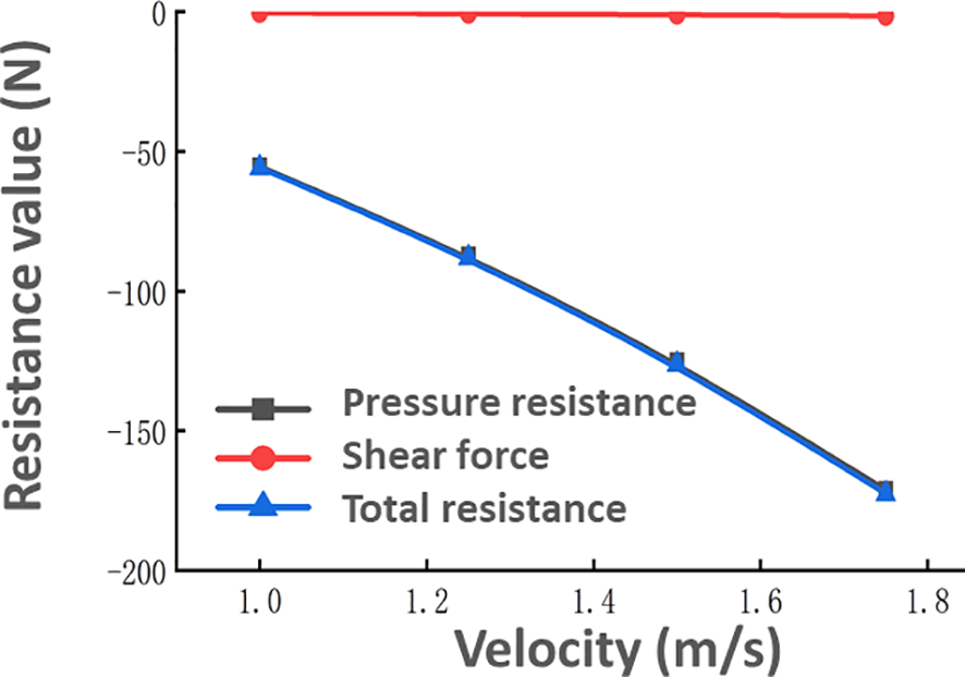
Figure 34 Lateral motion resistance.

In Figure 34, the resistance of the ROV transverse motion increases with the increase of velocity, and the pressure resistance occupies the main part of the total resistance. In lateral motion, there is a significant pressure difference between the frontal and backwater surfaces of the ROV, which is the main cause of the pressure resistance. Since the ROV is moving at a low velocity, the velocity gradient of the surrounding flow field is smaller, and the shear resistance caused by the velocity gradient of the flow field near the wall of the ROV is much smaller than the pressure resistance.

4.4 Data processing

4.4.1 Principles of data processing for stationary motion

Because the stationary motion is a uniform motion, the hydrodynamic term moving in all directions of the extension only has a velocity term and has nothing to do with the acceleration term. Simplifying the kinematic equations on the three axes yields Equation (18).

$\begin{array}{ll}\{\begin{array}{c}{F}_x=-X_{uu}{u}^2\\ F_y=-Y_{v\left|v\right|}\left|{(v^2)}^{\frac{1}{2}}\right|\\ F_z=-\left[Z_{w\left|w\right|}^{\text{'}}w\left|{(w^2)}^{\frac{1}{2}}\right|+Z_{ww}^{\text{'}}w\left|{(w^2)}^{\frac{1}{2}}\right|\right]\end{array}& (18)\end{array}$

In Equation (18): F_x, F_y, F_z are numerical calculation of the resistance value; $X_{uu,}^{\text{'}}$ $Z_{ww,}^{\text{'}}$ $Y_{v\left|v\right|,}^{\text{'}}$ $Z_{w\left|w\right|}^{\text{'}}$ are nonlinear hydrodynamic coefficients.

In order to facilitate data expression, the variables in the formula need to be dimensionless. Several variables in Equation (18) are dimensionless, as shown in Equation (19).

$$X_{uu}=\frac{\rho }{2}{L}^2{X}_{uu}^{\text{'}}, Y_{v\left|v\right|}=\frac{\rho }{2}{L}^2{Y}_{v\left|v\right|}^{\text{'}}$$

$\begin{array}{ll}{Z}_{w\left|w\right|}=\frac{\rho }{2}{L}^2{Z}_{w\left|w\right|}^{\text{'}}, Z_{ww}=\frac{\rho }{2}{L}^2{Z}_{ww}^{\text{'}}& (19)\end{array}$

In Equation: L for ROV length; ρ for the density of water. Bringing Equation (19) into Equation (18) gives a dimensionless expression, as shown in Equation (20).

$\begin{array}{ll}\{\begin{array}{c}{F}_x=-\frac{\rho }{2}{L}^2{X}_{uu}^{\text{'}}{u}^2\\ F_y=-\frac{\rho }{2}{L}^2{Y}_{v\left|v\right|}^{\text{'}}\left|{(v^2)}^{\frac{1}{2}}\right|\\ F_z=-\frac{\rho }{2}{L}^2\left[Z_{w\left|w\right|}^{\text{'}}w\left|{(w^2)}^{\frac{1}{2}}\right|+Z_{ww}^{\text{'}}w\left|{(w^2)}^{\frac{1}{2}}\right|\right]\end{array}& (20)\end{array}$

Considering the external characteristics of the ROV, when moving laterally, its resistance values in the positive and negative directions are the same. However, when the z-axis is moving, the resistance values of the rising (w<0) and sinking (w>0) movements are different, and the resistance coefficients are also different. The resistance to the z-axis motion is expressed as shown in Equation (21).

$\begin{array}{ll}=Z_{w\left|w\right|}w\left|w\right|+Z_{ww}ww=\{\begin{array}{c}(Z_{w\left|w\right|}+Z_{ww})w\left|w\right|,(w>0)\\ (Z_{w\left|w\right|}-Z_{ww})w\left|w\right|,(w<0)\end{array}& (21)\end{array}$

Further analysis can be obtained the expression of the coefficient $Z_{w\left|w\right|}$ and $Z_{ww}$ in Equation (22).

$$Z_{ww}=\frac{1}{2}\left(Z_{w\left|w\right|}{}^{(+)}+Z_{w\left|w\right|}{}^{(-)}\right)$$

$\begin{array}{ll}{Z}_{w\left|w\right|}=\frac{1}{2}(Z_{w\left|w\right|}{}^{(+)}-Z_{w\left|w\right|}{}^{(-)})& (22)\end{array}$

4.4.2 Fitting of the data

According to the above equation of motion, the data fitting results of hydrodynamic calculation are carried out by the least squares method, and MATLAB software is used in the data fitting, compared with the resistance curve in the simulation calculation, the fitting curve obtained by the least squares method is more accurate, as shown in Figures 35–37.

Figure 35

Figure 35 Resistance fitting curve.

Figure 36

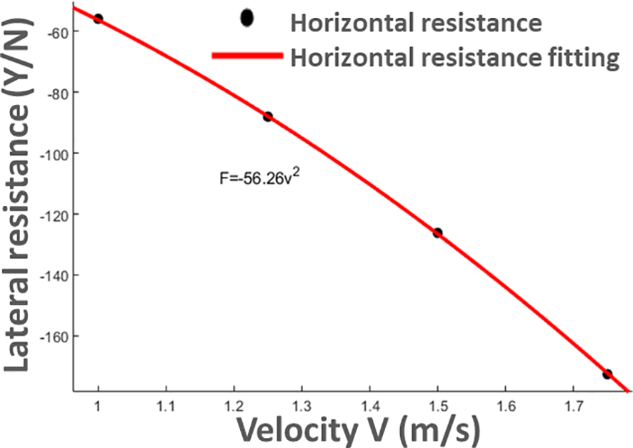
Figure 36 y-axis resistance fitting curve in the y-axis direction.

Figure 37

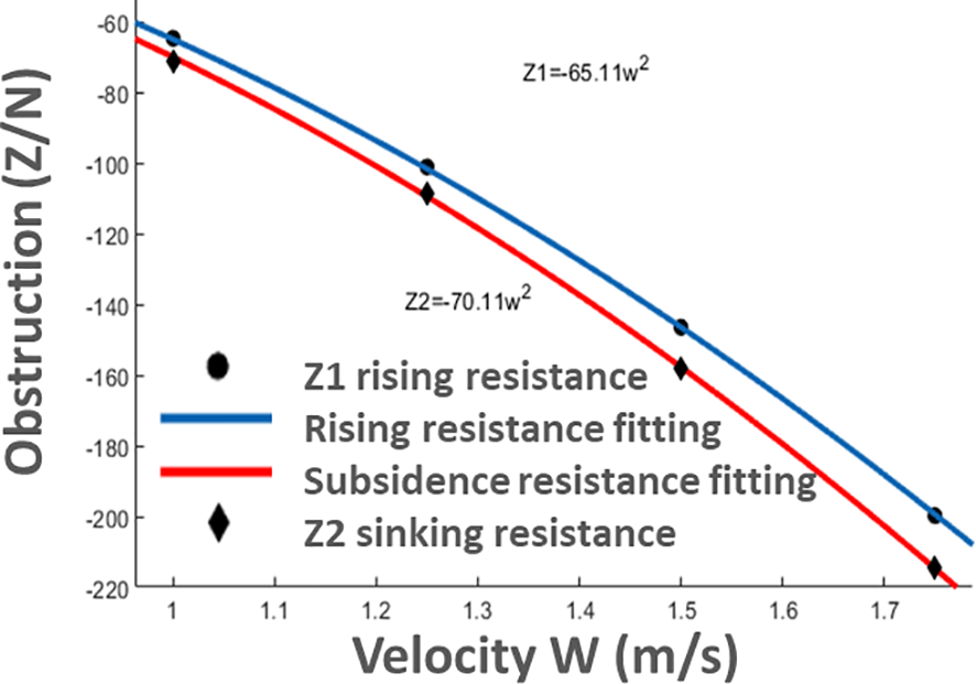
Figure 37 Fitting curve of ascending and sinking resistance.

The values of each hydrodynamic coefficient could be derived based on the functional expression of the curve fitted to the data. The hydrodynamic coefficients of a statistical type are shown in Table 13.

Table 13

Table 13 Statistics of hydrodynamic coefficients of steady motion.

5 Simulation calculation of the unsteady motion of the ROV

In the direct motion state, only the hydrodynamic coefficient related to the velocity can be obtained, and the hydrodynamic coefficient related to the acceleration cannot be obtained. In order to comprehensively analyze the motion of the ROV, it is not comprehensive to obtain only the coefficient related to the acceleration, and it is necessary to obtain the hydrodynamic coefficient of the acceleration term in order to accurately analyze the motion of the ROV.

5.1 The ROV model simplifies the computational domain division and boundary layer setting

5.1.1 Meshing and mesh-independent verification

5.1.1.1 Meshing

To analyze the unstable motion, it is essential to use overset meshes, which consist of two distinct sets of meshes that are separated independently and then nested and merged. When the overset mesh replicates intricate movement, the inner mesh propels the ROV to move in unison, while the outside mesh emulates the stationary motion inside the complicated movement. These two movements are interconnected to achieve the complex motion of the ROV. However, the use of an overset mesh necessitates the inclusion of two sets of meshes, resulting in a larger number of meshes. This increase is constrained by the limitations of computer performance. When employing the overset mesh calculation method, it is necessary to divide the mesh area into smaller sections in order to achieve greater precision. Ultimately, the determination of the number of meshes and the size of each mesh section should be based on a comprehensive assessment of calculation accuracy and computer performance. The mesh is divided into two areas, the inner mesh and the outer mesh, and in order to avoid the interpolation of the mesh affecting the calculation accuracy, the inner mesh must be set to ensure that it has a certain distance from the ROV surface. In this article, this distance is set to 0.25L. The outer mesh needs to be divided into multiple regions, which has the advantage of ensuring the calculation accuracy and effectively controlling the number of meshes. Here, the outer mesh is divided into four parts: the motion area, the encryption area, the transition area, and the outer mesh area. When meshing, you need to set the mesh base size for different areas, as shown in Table 14.

Table 14

Table 14 Meshing settings.

5.1.1.2 Mesh independence validation

After determining the mesh type and calculation domain, in order to ensure the accuracy of the simulation results and the calculation accuracy, in addition to considering the mesh type, the number of meshes is also an important influencing factor. Before performing numerical simulation calculations, mesh independence verification is required to determine the appropriate number of meshes. In this paper, six mesh quantities of 950,000, 1.17 million, 1.54 million, 1.95 million, 2.46 million, and 3 million are selected for verification. According to the set mesh type and boundary conditions, a working condition in the heave motion is selected for verification, the velocity is set to V=1.5m/s, the frequency is f=0.3125, and the simulation values of the force under different mesh numbers are counted, and the calculation results are shown in Table 15.

Table 15

Table 15 Vertical force of different meshes.

According to the analysis of the change of force and mesh number in Figure 38, the Lateral force decreases with the increase of the number of meshes, and the resistance value tends to be flat when the number of meshes is greater than 2.46 million. When the number of meshes is less than 2 million, the mesh size is large, the surface restoration degree of the mesh to the ROV is poor, and the gap between the simulated value and the experimental value is large. When the number of meshes is greater than 2.67 million, the mesh size is small, and the mesh can better restore the shape and flow field of the ROV, and the resistance value obtained is also more accurate. Considering the requirements of computer performance and computational accuracy, the final number of meshes in this paper is 2.67 million.

Figure 38

Figure 38 Force changes with the number of meshes.

5.2 Hydrodynamic calculations of planar motion mechanism

5.2.1 Definition and description of pure lateral motion

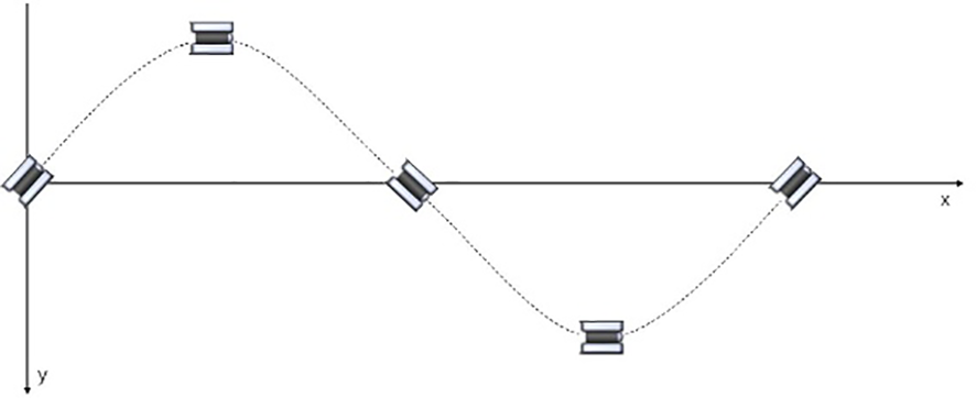
In the plane motion, there are two kinds of motion states, pure transverse motion and pure bow roll, in which the pure transverse motion is formed by the coupling of the uniform motion in the direction of the extended x-axis and the translational movement in the direction of the extended y-axis, and the motion is sinusoidally oscillating in the horizontal plane, and the angle between the bow and the x-axis is always zero. In the setting of this paper, according to the calculation results of the direct course resistance, the incoming flow velocity in the x-axis direction of the pure lateral motion is selected as V=1.5m/s. A schematic diagram of the motion of the pure lateral motion state, as shown in Figure 39.

Figure 39

Figure 39 Schematic diagram of pure swaying motion.

The equation of motion for a pure lateral motion is shown in Equation (23).

$\begin{array}{ll}\{\begin{array}{c}\eta =a\mathit{sin}\omega t\\ \psi =\dot{\psi }=0\\ v=\dot{\eta }=a\omega \mathit{cos}\omega t\\ \dot{v}=-a{\omega }^2\mathit{sin}\omega t\end{array}& (23)\end{array}$

In Equation (23), η—ROV lateral shift;

a —ROV Pure transverse amplitude;

ω —ROV Pure horizontal swing circle frequency;

$\psi 、\dot{\psi }$ —ROV Tilt angle and angular velocity about the z-axis;

$v、\dot{v}$ —ROV Transverse velocity and acceleration.

The Lateral force Y and the yaw moment N are expressed using the velocity and acceleration terms, and the force and moment expressions are shown in Equation (24).

$\begin{array}{ll}\{\begin{array}{c}Y=Y_{\dot{v}}\dot{v}+Y_{v}v+Y_0\\ N=N_{\dot{v}}\dot{v}+N_{v}v+N_0\end{array}& (24)\end{array}$

Bringing Equation (23) into Equation (24), the expression of force and moment can be expressed by Equation (25).

$\begin{array}{ll}\{\begin{array}{c}Y=Y_0-a{\omega }^2{Y}_{\dot{v}}\mathit{sin}\omega t+a\omega Y_v\mathit{cos}\omega t\\ N=N_0-a{\omega }^2{N}_{\dot{v}}\mathit{sin}\omega t+a\omega N_v\mathit{cos}\omega t\end{array}& (25)\end{array}$

In order to simplify the writing and facilitate the subsequent data fitting, Equation (25) is further simplified to obtain Equation (26).

$\begin{array}{ll}\{\begin{array}{c}Y=Y_0+Y_a\mathit{sin}\omega t+Y_b\mathit{cos}\omega t\\ N=N_0+N_a\mathit{sin}\omega t+N_b\mathit{cos}\omega t\end{array}& (26)\end{array}$

The expression of the relationship between (25) and the coefficient in Equation (26) is represented by Equation (27).

$$Y_a=-a{\omega }^2{Y}_{\dot{v}},Y_b=a\omega Y_v$$

$\begin{array}{ll}{N}_a=-a{\omega }^2{N}_{\dot{v}},N_b=a\omega N_v& (27)\end{array}$

The hydrodynamic coefficients of the pure lateral motion are dimensionless, and the results are shown in Equation (28).

$\begin{array}{ll}{Y}_{\dot{v}}{}^{\text{'}}=\frac{Y_{\dot{v}}}{\frac{1}{2}\rho L^3},Y_v{}^{\text{'}}=\frac{Y_v}{\frac{1}{2}\rho L^{2}U},N_{\dot{v}}{}^{\text{'}}=\frac{N_{\dot{v}}}{\frac{1}{2}\rho L^4},N_v{}^{\text{'}}=\frac{N_v}{\frac{1}{2}\rho L^{3}U}& (28)\end{array}$

The hydrodynamic coefficients that need to be obtained in pure lateral motion are shown in Table 16.

Table 16

Table 16 Hydrodynamic coefficients of pure transverse motion.

5.2.2 Post-processing and data analysis of pure lateral movements

In the pure traverse motion simulation, according to the motion analysis of the ROV, the motion of the ROV needs to be expressed through the functional equation. Pure transverse motion is formed by superimposing a constant velocity motion in the x-axis direction and a variable velocity motion in the y-axis. In this paper, the flow velocity V=1.5m/s is obtained, and the motion of the y-axis can be defined by the field function. The motion of the ROV in the y-axis direction is programmed, and the field function is written according to the equation of motion of the ROV to prepare for the subsequent ROV motion setting. The frequencies were f=0.2, 0.25, 0.3125 and 0.4 respectively. In this paper, the flow velocity is taken as V=1.5m/s, and for the amplitude a, a=0.15m is selected based on referring to the predecessors. In this paper, the simulation time is 4T (T is the motion period). For the time step, T/500-T/300 is generally taken in the simulation experiment, and the time step in this paper is set to T/400 considering the performance limitation of the computer. The step sizes and calculation times for the four working conditions are listed in Table 17.

Table 17

Table 17 Initial value setting.

For the simulation data in unsteady motion, the corresponding hydrodynamic coefficient can be obtained through data processing, and it is not appropriate to directly use the least squares method to process the simulation data because the lateral force and the yaw moment are periodically varying in the pure lateral motion. Previous studies have shown that accurate hydrodynamic coefficients can be obtained by processing the periodic data by Fourier expansion. The Fourier expansion is shown in Equations (29), (30).

$\begin{array}{ll}f(t)=\frac{a_0}{2}+{\sum }_{n=1}^{\infty }(a_n\mathit{cos}(\frac{n\pi t}{l})+b_n\mathit{sin}(\frac{n\pi t}{l}))& (29)\end{array}$

$\begin{array}{ll}\{\begin{array}{c}{a}_n=\frac{1}{l}{\displaystyle {\int }_{-l}^l}f(t)\mathit{cos}(\frac{n\pi t}{l})dt,(n=0, 1,\mathrm{2\dots })\\ b_n=\frac{1}{l}{\displaystyle {\int }_{-l}^l}f(t)\mathit{sin}(\frac{n\pi t}{l})dt,(n=0, 1,\mathrm{2\dots })\end{array}& (30)\end{array}$

Suppose the period is2l, because $\omega =\frac{2\pi }{T}=\frac{\pi }{l}$, then Equation (29) can be reduced to Equation (31).

$\begin{array}{ll}f(t)=\frac{a_0}{2}+a_1\mathit{cos}(\omega t)+b_1\mathit{sin}(\omega t)+{\sum }_{n=2}^{\infty }(a_n\mathit{cos}(n\omega t)+b_n\mathit{sin}(n\omega t))& (31)\end{array}$

Because n=2 and later terms have much less than the coefficient values a₁ and a₂, in omitted n=2 and after the item, Equation (32) can be obtained.

$\begin{array}{ll}f(t)=\frac{a_0}{2}+a_1\mathit{cos}(\omega t)+b_1\mathit{sin}(\omega t)& (32)\end{array}$

Using the Fourier theorem to expand Equation (30), we get Equations (33), (34).

For Lateral force Y:

$\begin{array}{ll}\{\begin{array}{c}{b}_1=Y_a=-a{\omega }^2{Y}_{\dot{v}}=\frac{1}{l}{\displaystyle {\int }_{-l}^l}f(t)\mathit{sin}(\omega t)dt\\ a_1=Y_b=a\omega Y_v=\frac{1}{l}{\displaystyle {\int }_{-l}^l}f(t)\mathit{cos}(\omega t)dt\end{array}& (33)\end{array}$

For yaw moment N:

$\begin{array}{ll}\{\begin{array}{c}{b}_1^{\text{'}}=N_a=-a{\omega }^2{N}_{\dot{v}}=\frac{1}{l}{\displaystyle {\int }_{-l}^l}f(t)\mathit{sin}(\omega t)dt\\ a_1^{\text{'}}=N_b=a\omega N_v=\frac{1}{l}{\displaystyle {\int }_{-l}^l}f(t)\mathit{cos}(\omega t)dt\end{array}& (34)\end{array}$

The simulation calculation of working conditions at different frequencies is carried out, and the stable data that can be used for data processing are selected from the simulation data, and the simulation data can be found to be stable after the second cycle through experiments. In this paper, the data of the third cycle are selected for analysis and processing, and the simulation data of the third cycle is fitted by Fourier series using MATLAB software. The coefficients under the Fourier series were obtained by fitting the curves, and the fitting coefficients under different working conditions were counted, and the statistical results are shown in Table 18.

Table 18

Table 18 Pure sway calculation data.

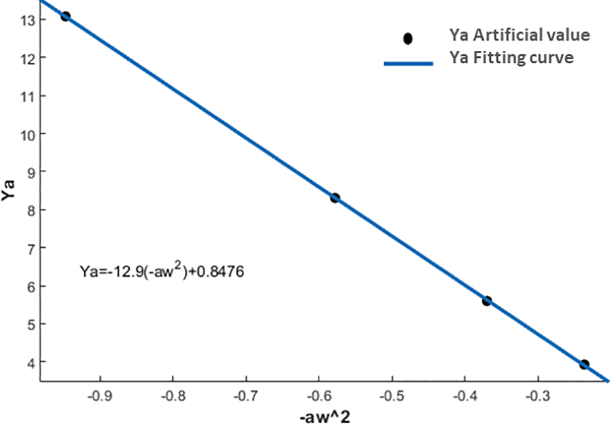
According to Equations (33), (34), the data in the table are fitted by MATLAB software, and the hydrodynamic coefficients of the ROV in the unsteady state can be obtained through the quadratic fitting, and the fitting results are shown in Figures 40–43.

Figure 40

Figure 40 Ya fitting curve.

Figure 41

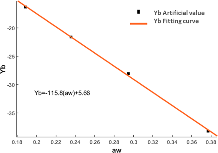
Figure 41 Yb fitting curve.

Figure 42

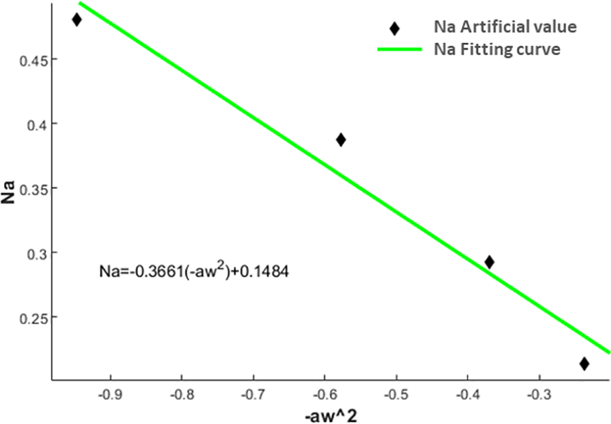
Figure 42 Na fitting curve.

Figure 43

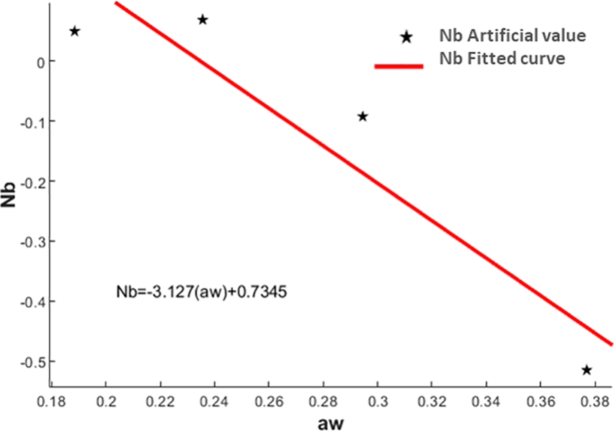
Figure 43 Nb fitting curve.

The hydrodynamic coefficients obtained are shown in Table 19.

Table 19

Table 19 Statistics of pure transverse hydrodynamic coefficients.

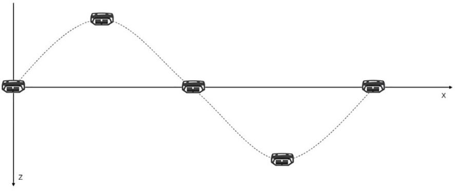
5.2.3 Definition and description of pure yaw motion

Pure yaw motion refers to superimposing a bow motion on the basis of pure lateral motion, and ensuring that the direction of the velocity of the ROV movement is tangent to the trajectory. And in the follower coordinate system, the lateral motion velocity and lateral acceleration of the follower coordinate system are zero. Through the pure yaw motion experiment, the hydrodynamic coefficients of the underwater robot in relation to angular velocity and angular acceleration can be obtained. As with the pure lateral motion, the incoming velocity is set to V=1.5m/s in this paper. A schematic diagram of a pure yaw motion is shown in Figure 44.

Figure 44

Figure 44 Pure yow motion.

The pure yaw motion can be expressed by the equation of motion, which can be expressed as Equation (35).

$\begin{array}{ll}\{\begin{array}{c}\psi ={\psi }_0\mathit{sin}(\omega t)\\ r=\dot{\psi }={\psi }_0\omega \mathit{cos}(\omega t)\\ \dot{r}=-{\psi }_0{\omega }^2\mathit{sin}(\omega t)\\ v=\dot{v}=0\end{array}& (35)\end{array}$

In Equation (35):

$\psi$—amplitude of pure yaw motion;

${\psi }_0$—amplitude of pure bow shake movement;

$\omega$—the circular frequency of the pure yaw motion;

$r,\dot{r}$—the angle of rotation about the z-axis and the angular velocity;

$v,\dot{v}$—Lateral velocity and acceleration.

After analyzing the pure yaw motion of the ROV, the lateral force Y and the yaw moment N are expressed by angular velocity and angular acceleration, and the expressions of force and moment are obtained, as shown in Equation (36).

$\begin{array}{ll}\{\begin{array}{c}Y=Y_0+Y_{\dot{r}}\dot{r}+Y_{r}r\\ N=N_0+N_{\dot{r}}\dot{r}+N_{r}r\end{array}& (36)\end{array}$

If the parametric expression in Equation (54) is brought into Equation (55), then the expression of force and moment can be expressed as Equation (37).

$\begin{array}{ll}\{\begin{array}{c}Y=Y_0-{\psi }_0{\omega }^2{Y}_{\dot{r}}\mathit{sin}\omega t+{\psi }_0\omega Y_r\mathit{cos}\omega t\\ N=N_0-{\psi }_0{\omega }^2{N}_{\dot{r}}\mathit{sin}\omega t+{\psi }_0\omega N_r\mathit{cos}\omega t\end{array}& (37)\end{array}$

In order to simplify the writing and facilitate the subsequent data processing, Equation (37) is simplified to obtain Equation (38).

$\begin{array}{ll}\{\begin{array}{c}Y=Y_0+Y_c\mathit{sin}\omega t+Y_d\mathit{cos}\omega t\\ N=N_0+N_c\mathit{sin}\omega t+N_d\mathit{cos}\omega t\end{array}& (38)\end{array}$

The relationship between Equation (36) and the coefficient of the corresponding term in Equation (38) can be expressed by Equation (39).

$\begin{array}{ll}{Y}_c=-{\psi }_0{\omega }^2{Y}_{\dot{v}},Y_d={\psi }_0\omega Y_v& (39)\end{array}$

The hydrodynamic coefficients were dimensionless respectively, and the results are shown in Equation (40).

$\begin{array}{ll}{Y}_{\dot{r}}{}^{\text{'}}=\frac{Y_{\dot{r}}}{\frac{1}{2}\rho L^4},Y_r{}^{\text{'}}=\frac{Y_r}{\frac{1}{2}\rho L^{3}U},N_{\dot{r}}{}^{\text{'}}=\frac{N_{\dot{r}}}{\frac{1}{2}\rho L^5},N_r{}^{\text{'}}=\frac{N_r}{\frac{1}{2}\rho L^{4}U}& (40)\end{array}$

The hydrodynamic coefficients that need to be obtained in a pure bow motion are shown in Table 20.

Table 20

Table 20 Pure yaw motion coefficients.

5.2.4 Post-processing and data analysis of pure bow motion

Initially, it is necessary to establish a fresh coordinate system whereby the point of origin coincides with the location of the center of gravity. The equation of motion of the pure bow jolt should be programmed first, as with the pure yaw motion, and the code acquired by programming is saved in the field function to prepare for the succeeding motion settings. Following the completion of the overlap area’s motion configuration, simulation and calculation are required for the four working conditions that were selected: f=0.2, 0.25, 0.3125, and 0.4. The entering velocity in pure bow motion is fixed at V=1.5m/s. The time step size and calculation time remain the same as those used for pure sideways motion. For a pure yaw motion, the Lateral force and the yaw moment are expanded in Fourier series, as shown in Equations (41), (42).

For Lateral force Y:

$\begin{array}{ll}\{\begin{array}{c}{c}_1=Y_c=-{\psi }_0{\omega }^2{Y}_{\dot{r}}=\frac{1}{l}{\displaystyle {\int }_{-l}^l}f(t)\mathit{sin}(\omega t)dt\\ d_1=Y_d={\psi }_0\omega Y_r=\frac{1}{l}{\displaystyle {\int }_{-l}^l}f(t)\mathit{cos}(\omega t)dt\end{array}& (41)\end{array}$

For yaw moment N:

$\begin{array}{ll}\{\begin{array}{c}{c}_1^{\text{'}}=N_c=-{\psi }_0{\omega }^2{N}_{\dot{r}}=\frac{1}{l}{\displaystyle {\int }_{-l}^l}f(t)\mathit{sin}(\omega t)dt\\ d_1^{\text{'}}=N_d={\psi }_0\omega N_r=\frac{1}{l}{\displaystyle {\int }_{-l}^l}f(t)\mathit{cos}(\omega t)dt\end{array}& (42)\end{array}$

As with the pure lateral motion, the data of the third period are selected for data fitting, and the fitting coefficients under different working conditions in the Fourier fitting are counted, as shown in Table 21.

Table 21

Table 21 Calculation data of pure yaw motion.

According to Equations (41), (42), the data in the table are quadratically fitted by MATLAB software, and the hydrodynamic coefficients of pure yaw motion can be obtained through quadratic fitting, and the results of quadratic fitting are shown in Figures 44–48.

Figure 45

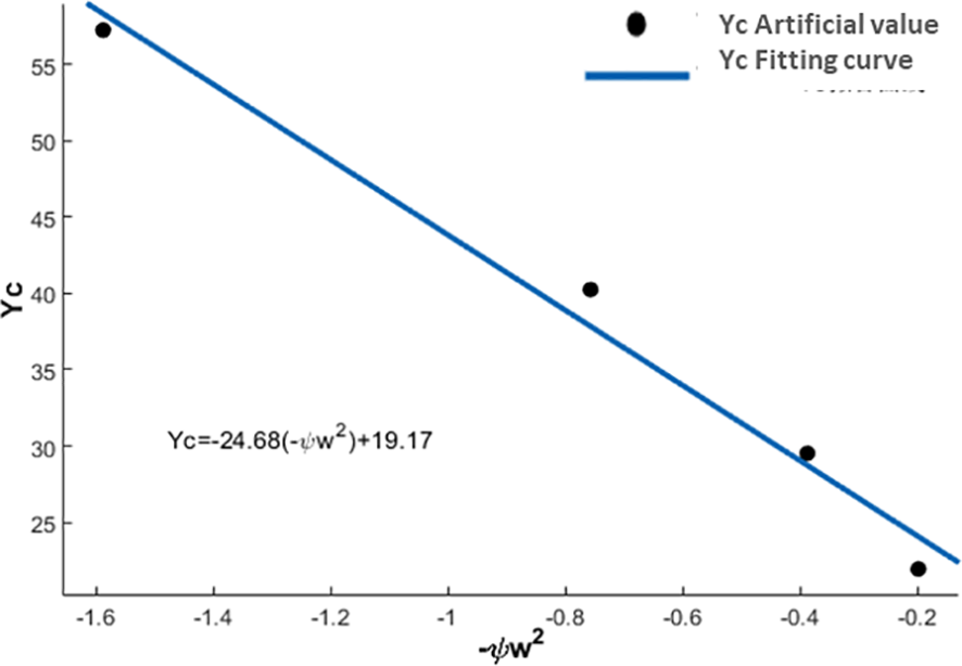
Figure 45 Yc fitting curve.

Figure 46

Figure 46 Yd fitting curve.

Figure 47

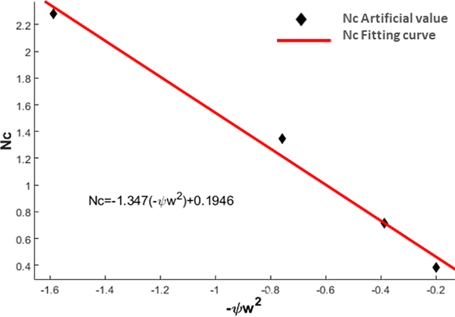
Figure 47 Nc fitting curve.

Figure 48

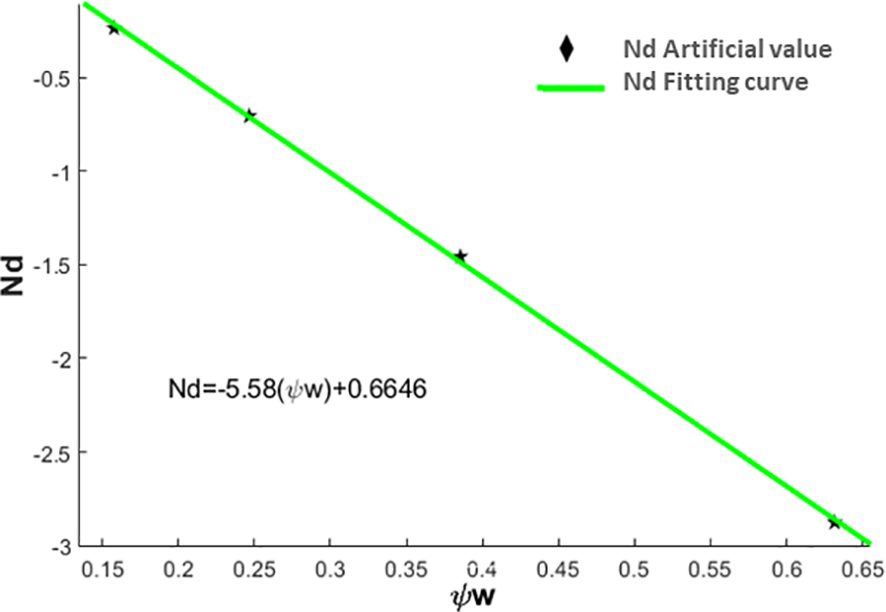
Figure 48 Nd fitting curve.

The hydrodynamic coefficients and dimensionless coefficients obtained by quadratic fitting are counted, and the statistical results are shown in Table 22.

Table 22

Table 22 Statistics of pure motion hydrodynamic coefficient.

5.3 Hydrodynamic calculation of the vertical plane motion mechanism

5.3.1 Definition and description of pure heave motion

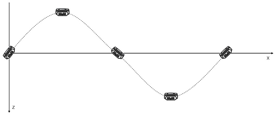
The motion of the vertical plane mechanism includes two kinds of motions: pure heave and pure pitching, and the pure heave motion refers to the combined motion formed by the superposition of the uniform motion of the x-axis and the variable velocity motion in the z-axis direction, and the trajectory of the pure heave motion in the xoz plane is a sine wave, and the angle between the bow and the x-axis of the ROV is always kept at zero degrees. In this paper, the constant motion of the extended x-axis is set to V=1.5m/s. A schematic diagram of the pure heave motion is shown in Figure 49.

Figure 49

Figure 49 Pure heave motion.

The pure heave motion can be expressed by a parametric equation as shown in Equation (43).

$\begin{array}{ll}\{\begin{array}{c}\zeta =a\mathit{sin}(\omega t)\\ \theta =\dot{\theta }=0\\ w=\dot{\zeta }=a\omega \mathit{cos}(\omega t)\\ \dot{w}=-a{\omega }^2\mathit{sin}(\omega t)\end{array}& (43)\end{array}$

In Equation (43):

$\zeta$—ROV vertical displacement;

a—penchant amplitude;

$\omega$—circular frequency;

$\theta , \dot{\theta }$—angular velocity about the y-axis;

$w, \dot{w}$—Vertical velocity and acceleration.

The vertical force Z and the pitching moment M are expressed by the terms velocity and acceleration, and the expression for the force and moment is shown in Equation (44).

$\begin{array}{ll}\{\begin{array}{c}Z=Z_0+Z_{\dot{w}}\dot{w}+Z_{w}w\\ M=M_0+M_{\dot{w}}\dot{w}+M_{w}w\end{array}& (44)\end{array}$

Transporting Equation (43) into Equation (44) allows for a pure equation of motion for heave and heave, as shown in Equation (45).

$\begin{array}{ll}\{\begin{array}{c}Z=Z_0-a{\omega }^2{Z}_{\dot{w}}\mathit{sin}(\omega t)+a\omega Z_w\mathit{cos}(\omega t)\\ M=M_0-a{\omega }^2{M}_{\dot{w}}\mathit{sin}(\omega t)+a\omega M_w\mathit{cos}(\omega t)\end{array}& (45)\end{array}$

In order to simplify the writing and facilitate subsequent data processing, Equation (45) is simplified, and the simplified equation is shown in Equation (46).

$\begin{array}{ll}\{\begin{array}{c}Z=Z_0{\text{+Z}}_1\mathit{sin}\omega t+Z_2\mathit{cos}\omega t\\ M=M_0+M_1\mathit{sin}\omega t+M_2\mathit{cos}\omega t\end{array}& (46)\end{array}$

The expression of the relationship between Equation (45) and the coefficient of the corresponding term in Equation (46) is represented by Equation (47).

$$Z_1=-a{\omega }^2{Z}_{\dot{w}},Z_2=a\omega Z_w$$

$\begin{array}{ll}{M}_1=-a{\omega }^2{M}_{\dot{w}},W_2=a\omega M_w& (47)\end{array}$

The hydrodynamic coefficients in Equation (45) are dimensionless respectively, and the dimensionless mode is shown in Equation (48).

$\begin{array}{ll}{Z}_{\dot{w}}^{\text{'}}=\frac{Z_{\dot{w}}}{\frac{1}{2}\rho L^3},Z_w{}^{\text{'}}=\frac{Z_w}{\frac{1}{2}\rho L^{2}U},M_{\dot{w}}{}^{\text{'}}=\frac{M_{\dot{w}}}{\frac{1}{2}\rho L^4},M_w{}^{\text{'}}=\frac{M_w}{\frac{1}{2}\rho L^{3}U}& (48)\end{array}$

The hydrodynamic coefficients that need to be obtained in the pure heave and heave are shown in Table 23.

Table 23

Table 23 Pure heave hydrodynamic coefficient.

5.3.2 Post-processing and data analysis of pure heave motion

In pure heave motion, the trajectory of the ROV in the xoz plane is a sine wave. As with pure transverse motion, the sinusoidal motion is decomposed into a uniform motion in the direction of the x-axis and a variable velocity motion in the direction of the z-axis. For the constant velocity motion in the x-axis direction, the velocity V=1.5m/s, and the variable velocity motion in the z-axis direction is represented by a mathematical function.

In order to facilitate the setting of the velocity of the variable velocity movement, it is necessary to encode in the field function and write the expression of the function that controls the variable velocity motion. Once the code has been programmed in the field function, you can continue to set the variable velocity motion in the z-axis direction of the overlap area. After the motion setting of the overlap area is completed, four working conditions with frequencies of f=0.2, 0.25, 0.3125 and 0.4 are selected for calculation. The incoming velocity is set to V=1.5m/s, and the amplitude is consistent with the pure lateral motion, and a=0.15m is selected. In order to obtain stable data, the calculation period is selected as four periods, and the data of the third period is selected for data fitting. Time step, set to T/400.

Considering the periodicity of the data, it is necessary to use the Fourier series expansion for the data obtained in the simulation calculation, and the Fourier series expansion for the vertical force Z and the pitching moment M is shown in Equations (48), (59).

For the vertical force Z:

$\begin{array}{ll}\{\begin{array}{c}{e}_1=Z_1=-a{\omega }^2{Z}_{\dot{w}}=\frac{1}{l}{\displaystyle {\int }_{-l}^l}f(t)\mathit{sin}(\omega t)dt\\ f_1=Z_2=a\omega Z_w=\frac{1}{l}{\displaystyle {\int }_{-l}^l}f(t)\mathit{cos}(\omega t)dt\end{array}& (49)\end{array}$

For the yaw moment M:

$\begin{array}{ll}\{\begin{array}{c}{e}_1^{\text{'}}=M_1=-a{\omega }^2{M}_{\dot{w}}=\frac{1}{l}{\displaystyle {\int }_{-l}^l}f(t)\mathit{sin}(\omega t)dt\\ f_1^{\text{'}}=M_2=a\omega M_w=\frac{1}{l}{\displaystyle {\int }_{-l}^l}f(t)\mathit{cos}(\omega t)dt\end{array}& (50)\end{array}$

After calculating the working conditions at different frequencies, the data of the third period were selected from the obtained data for processing, and the data were fitted by Fourier series using MATLAB software. The coefficients of the fitting curves under different working conditions are statistically shown in Table 24.

Table 24

Table 24 Pure heave calculation data.

According to Equations (49), (50), the data in the table are fitted by MATLAB software, and the hydrodynamic coefficients in the pure heave motion can be obtained through the secondary fitting, and the results of the second fitting are shown in Figures 50–53.

Figure 50

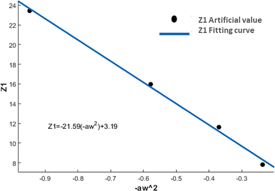
Figure 50 Z1 fitting curve.

Figure 51

Figure 51 Z2 fitting curve.

Figure 52

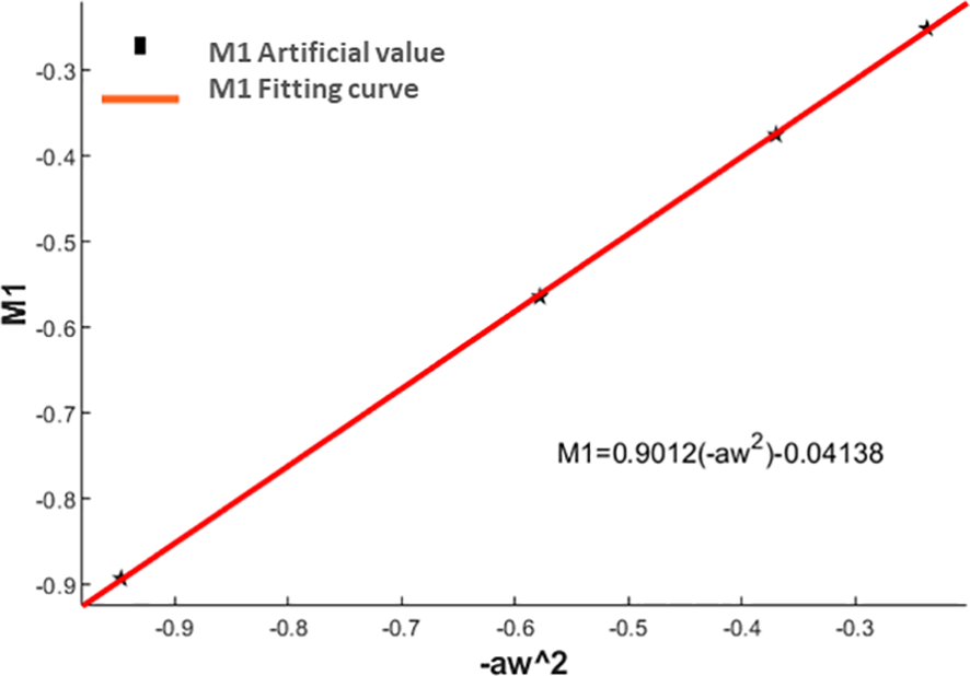
Figure 52 M1 fitting curve.

Figure 53

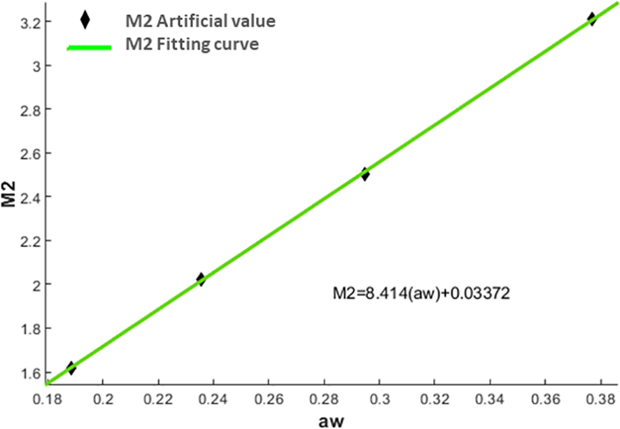
Figure 53 M2 fitting curve.

The hydrodynamic coefficients obtained by quadratic fitting and their dimensionless values are statistically analyzed, and the statistical results are shown in Table 25.

Table 25

Table 25 Statistics of pure heave hydrodynamic coefficient.

5.3.3 Definition and description of pure pitching motion

Pure pitch motion is a combination of a rotational motion about the y-axis on the basis of pure lateral motion. In motion, the direction of velocity of the ROV is tangent to the sinusoidal trajectory. In the follow-up coordinate system, the vertical velocity and acceleration of the ROV are zero. With pure pitching motion, the hydrodynamic coefficients related to angular velocity and angular acceleration of the underwater robot can be obtained, assuming that the velocity of the moving flow is V=1.5m/s. A schematic diagram of pure pitch motion is shown in Figure 54.

Figure 54

Figure 54 Pure pitch motion.

The pure pitch motion of the ROV can be expressed by the parametric equation, as shown in Equation (51).

$\begin{array}{ll}\{\begin{array}{c}\theta ={\theta }_0\mathit{sin}(\omega t)\\ w=\dot{w}=0\\ q=\dot{\theta }={\theta }_0\omega \mathit{cos}(\omega t)\\ \dot{q}=-{\theta }_0{\omega }^2\mathit{sin}(\omega t)\end{array}& (51)\end{array}$

In Equation (51):

$\theta$—Pitch angle;

${\theta }_0$—Pitching motion amplitude;

$\omega$—Circular frequency;

$q, \dot{q}$—Angle and angular velocity about the y-axis;

$w, \dot{w}$—Vertical velocity and acceleration.

The equations for the ROV pitch moment M and the vertical force Z can be expressed by the pitch angle and the pitch angular velocity, as shown in Equation (52).

$\begin{array}{ll}\{\begin{array}{c}Z=Z_0+Z_{\dot{q}}\dot{q}+Z_q\\ M=M_0+M_{\dot{q}}\dot{q}+M_q\end{array}& (52)\end{array}$

Bringing the equation of pure pitch motion into Equation (52) gives Equation (53).

$\begin{array}{ll}\{\begin{array}{c}Z=Z_0-{\theta }_0{\omega }^2{Z}_{\dot{q}}\mathit{sin}(\omega t)+{\theta }_0\omega Z_q\mathit{cos}(\omega t)\\ M=M_0-{\theta }_0{\omega }^2{M}_{\dot{q}}\mathit{sin}(\omega t)+{\theta }_0\omega M_q\mathit{cos}(\omega t)\end{array}& (53)\end{array}$

In order to simplify the writing and facilitate the subsequent data processing, Equation (53) is simplified to obtain Equation (54).

$\begin{array}{ll}\{\begin{array}{c}Z=Z_0{\text{+Z}}_3\mathit{sin}\omega t+Z_4\mathit{cos}\omega t\\ M=M_0+M_3\mathit{sin}\omega t+M_4\mathit{cos}\omega t\end{array}& (54)\end{array}$

The relationship between Equation (53) and the coefficient of the corresponding term in Equation (54) can be expressed by Equation (55).

$$Z_3=-{\theta }_0{\omega }^2{Z}_{\dot{q}},Z_4={\theta }_0\omega Z_q$$

$\begin{array}{ll}{M}_3=-{\theta }_0{\omega }^2{M}_{\dot{q}},W_4={\theta }_0\omega M_q& (55)\end{array}$

The hydrodynamic coefficient of pure pitching motion and its dimensionless value are shown in Equation (56).

$\begin{array}{ll}{Z}_{\dot{q}}^{\text{'}}=\frac{Z_{\dot{q}}}{\frac{1}{2}\rho L^4},Z_q{}^{\text{'}}=\frac{Z_q}{\frac{1}{2}\rho L^{3}U},M_{\dot{q}}{}^{\text{'}}=\frac{M_{\dot{q}}}{\frac{1}{2}\rho L^5},M_q{}^{\text{'}}=\frac{M_q}{\frac{1}{2}\rho L^{4}U}& (56)\end{array}$

The hydrodynamic coefficients that need to be obtained in pure pitching and sinking are shown in Table 26.

Table 26

Table 26 Pure pitch hydrodynamic coefficients.

5.3.4 Post-processing and data analysis of pure pitching movements

Pure pitch motion is made by superimposing a rotational angular velocity on the basis of pure heave motion, and in pure pitch motion, the trajectory of the center of gravity is a sine wave. In this paper, the flow velocity is set to V=1.5m/s, and the variable velocity motion in the z-axis direction is set to be the same as the pure heave motion. In addition, an angular acceleration needs to be superimposed on the ROV, and the angular acceleration expression is shown in Equation (57).

$\begin{array}{ll}\{\begin{array}{c}{\theta }_0=\frac{a\omega }{V}\\ q=\dot{\theta }={\theta }_0\omega \mathit{cos}(\omega t)=\frac{a{\omega }^2}{V}\mathit{cos}(\omega t)\end{array}& (57)\end{array}$

In the original pitch motion simulation calculation, as with the pure heave motion, the pure pitch equation of motion must be programmed first. The code that results from this programming is then saved in the entry function to set up the future motion settings. Following the completion of the overlap area’s motion setting procedure, four operating conditions—f=0.2, 0.25, 0.3125, and 0.4—are chosen for simulation computations. Since the amplitude is consistent with the pure heave motion and the incoming flow velocity of V=1.5 m/s, a= 0.15 m is chosen. The calculating period is chosen to consist of four periods in order to provide steady data; the third period’s data is chosen for data fitting. Set the time step to T/400. The step size and calculation period parameters are shown in Table 25. The extension of the Fourier series of the data received via simulation is required due to the periodic character of the data: the vertical force Z and pitching moment M Fourier series expansions are presented in Equations (58), (59).

For the vertical force Z:

$\begin{array}{ll}\{\begin{array}{c}{e}_2=Z_3=-{\theta }_0{\omega }^2{Z}_{\dot{q}}=\frac{1}{l}{\displaystyle {\int }_{-l}^l}f(t)\mathit{sin}(\omega t)dt\\ f_2=Z_4={\theta }_0\omega Z_q=\frac{1}{l}{\displaystyle {\int }_{-l}^l}f(t)\mathit{cos}(\omega t)dt\end{array}& (58)\end{array}$

For yaw moment M:

$\begin{array}{ll}\{\begin{array}{c}{e}_2^{\text{'}}=M_3=-{\theta }_0{\omega }^2{M}_{\dot{q}}=\frac{1}{l}{\displaystyle {\int }_{-l}^l}f(t)\mathit{sin}(\omega t)dt\\ f_2^{\text{'}}=M_4={\theta }_0\omega M_q=\frac{1}{l}{\displaystyle {\int }_{-l}^l}f(t)\mathit{cos}(\omega t)dt\end{array}& (59)\end{array}$

Following the calculation of operating conditions at various frequencies, the data from the third cycle had been selected for analysis and processing. The MATLAB program was then used to fit the data using Fourier series. The statistical analysis of the Fourier fitting yields the coefficients of the fitting curves, which are shown in Table 27.

Table 27

Table 27 Pure heave calculation data.

According to Equations (58), (59), the data in the table were re-fitted by MATLAB software, and the fitting results are shown in Figures 55–58.

Figure 55

Figure 55 Z3 fitting curve.

Figure 56

Figure 56 Z4 fitting curve.

Figure 57

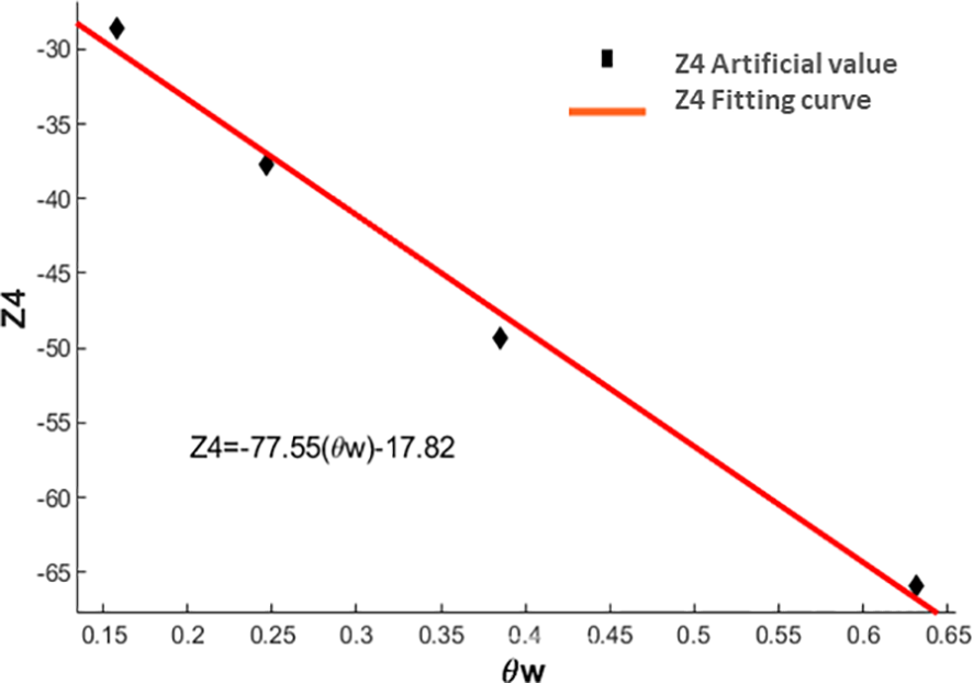
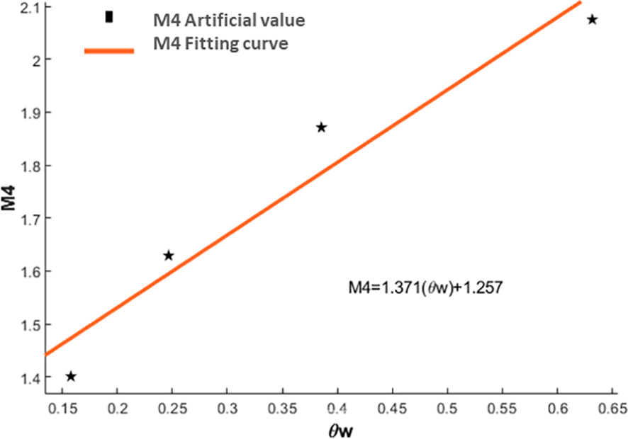
Figure 57 M3 fitting curve.

Figure 58

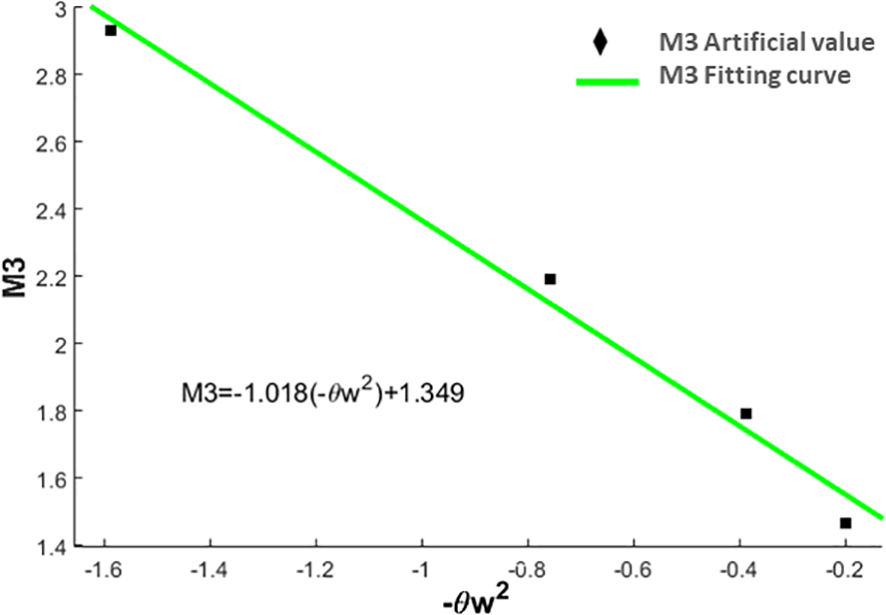
Figure 58 M4 fitting curve.

The statistically solved hydrodynamic coefficient of pure pitching motion and its dimensionless value, and the numerical statistical results are shown in Table 28.

Table 28

Table 28 Statistics of pure pitch hydrodynamic coefficients.

6 Conclusion

In summary, the ROV’s asymmetry results in an obvious disparity in pressure resistance between the forward and backward sailing, ascending and descending motions, and this disparity becomes significantly greater as the velocity increased. The relationship between pressure resistance and pressure resistance is closely related to the shape of the ROV model. Therefore, when designing the ROV, attention should be taken to ensure that the shape is as symmetrical as possible in order to achieve optimal hydrodynamic performance. Through a comparative and analytical analysis of the calculated and experimental values of the SUBOFF model, the reliability of the simulation process used in this paper is confirmed. Furthermore, the process is extended to the simulation calculation of the ROV model, enabling it to complete the ROV model simulation experiment and yield high-quality experimental results. This work also confirms that the unstable motion of the ROV can be simulated using the technique of superimposing the field function of the overset mesh, with satisfactory simulation results.

By analyzing data, we can derive some of the ROV’s hydrodynamic coefficients; they will serve as a foundation for future maneuverability tests and will cut down on the time it takes to develop the ROV. In ROV hydrodynamic modeling simulations, simulations can help predict the performance of ROVs under various constraint conditions and optimize their design and operation before actual deployment. They can also assist in evaluating the impact of different constraints on ROVs, such as maneuverability and stability under varying depths, water flow conditions, and workloads. By conducting simulation experiments, the costs and risks associated with physical testing can be reduced, while providing reliable data to guide the design and operation of ROVs.

Although the hydrodynamic calculation of ROV is performed in this study, no approximate formula for the hydrodynamic calculation of ROV is developed in this paper owing to experimental equipment limitations and computation time limitations. Further comparisons between the experimental data and the hydrodynamic coefficients found in this study are necessary. Future research may investigate the impact of various mesh types and mesh numbers on hydrodynamic computing efficiency; nevertheless, this paper’s meshing verification still has some holes due to computational restrictions.

Data availability statement

The original contributions presented in the study are included in the article/supplementary material. Further inquiries can be directed to the corresponding author.

Author contributions

DZ: Writing – original draft, Writing – review & editing. BZ: Writing – original draft, Writing – review & editing. YZ: Investigation, Validation, Visualization, Writing – review & editing. NZ: Writing – original draft, Writing – review & editing.

Funding

The author(s) declare financial support was received for the research, authorship, and/or publication of this article. This study was financially supported by Program for Scientific Research Start-up Funds of Guangdong Ocean University (060302072101), Comparative Study and Optimization of Horizontal Lifting of Subsea Pipeline (2021E05011), China Scholarship Council (CSC202306320084).

Conflict of interest

The authors declare that the research was conducted in the absence of any commercial or financial relationships that could be construed as a potential conflict of interest.

Publisher’s note

All claims expressed in this article are solely those of the authors and do not necessarily represent those of their affiliated organizations, or those of the publisher, the editors and the reviewers. Any product that may be evaluated in this article, or claim that may be made by its manufacturer, is not guaranteed or endorsed by the publisher.

Glossary

References

Cepeda S. F. M., MaChado F. S. D. M., Barbosa S. H. F., Moreira D. S. S., Almansa M. J. L., Souza M. L., et al. (2023). Exploring autonomous and remotely operated vehicles in offshore structure inspections. J. Mar. Sci. Eng. 11, 2172. doi: 10.3390/jmse11112172

CrossRef Full Text | Google Scholar

Chin C., Lau M. (2012). Modeling and testing of hydrodynamic damping Model for a complex-shaped remotely-operated vehicle for control. J. Mar. Sci. Appl. 11, 150–163. doi: 10.1007/s11804-012-1117-2

CrossRef Full Text | Google Scholar

Christophe V. (2023). Unmotorize ROV gripper to catch profiling floats. Ocean Eng. 288, 116013. doi: 10.1016/j.oceaneng.2023.116013

CrossRef Full Text | Google Scholar

Dalibor I., Marcin S. (2024). Assessing damage and predicting future risks: A study of the Schilling Titan 4 manipulator on work class ROVs in offshore oil and gas industry. Ocean Eng. 291, 116282. doi: 10.1016/j.oceaneng.2023.116282

CrossRef Full Text | Google Scholar

Fan S.-b., Lian L., Ren P. (2012). Research on hydrodynamics model test for deep sea open- framed remotely operated vehicle. China Ocean Eng. 26, 329–339. doi: 10.1007/s13344-012-0025-1

CrossRef Full Text | Google Scholar

Manimaran R. (2022). Hydrodynamic investigations on the performance of an underwater remote operated vehicle under the wave using OpenFOAM. Ships Offshore Structures 17, 2186–2202. doi: 10.1080/17445302.2021.1979921

CrossRef Full Text | Google Scholar

Mingjie L., Caoyang Y., Xiaochao Z., Chunhu L., Lian L. (2023). Fuzzy adaptive trajectory tracking control of work-class ROVs considering thruster dynamics. Ocean Eng. 267, 113232. doi: 10.1016/j.oceaneng.2022.113232

CrossRef Full Text | Google Scholar

Ren F., Hu Q. (2023). ROV sliding mode controller design and simulation. Processes 11, 2359. doi: 10.3390/pr11082359

CrossRef Full Text | Google Scholar

Selig G. M., Drazen J. C., Auster P. J., Mundy B. C., Kelley C. D. (2023). Distribution and structure of deep-sea demersal fish assemblages across the central and western Pacific Ocean using data from undersea imagery#13. Front. Mar. Sci. 10, 3389. doi: 10.3389/fmars.2023.1219368

CrossRef Full Text | Google Scholar

Skorpa S. (2012). Numerical Simulation of Flow Around Remotely Operated Vehicle (ROV) (Trondheim: Norwegian University of Science and Technology).

Google Scholar

Tanveer A., Ahmad M. S. (2023). Genetic-algorithm-based proportional integral controller (GAPI) for ROV steering control†. Eng. Proc. 32, 3390. doi: 10.3390/engproc2023032004

CrossRef Full Text | Google Scholar

Whitcomb L. L., Yoerger D. R. (1993). “A new distributed real-time control system for the Jason underwater robot,” in Proceedings of the IEEE/RSJ International Workshop on Intelligent Robots and Systems, vol. 1. (IEEE, Yokohama, Japan), 368–374.

Google Scholar

Zhang D., Wang X., Zhao M., Hong L., Li X. (2023). Numerical investigation on hydrodynamic characteristics and drag influence of an open-frame remotely operated underwater vehicle. J. Mar. Sci. Eng. 11, 2143. doi: 10.3390/jmse11112143

CrossRef Full Text | Google Scholar

Zhao B., Yun Y., Hu F., Sun J., Wu D., Huang B. (2022). Hydrodynamic coefficients of the DARPA SUBOFF AFF-8 in rotating arm maneuver: Part I: Test technology and validation. Ocean Eng. 266, 113148. doi: 10.1016/j.oceaneng.2022.113148

CrossRef Full Text | Google Scholar

Zhao B., Yun Y., Hu F., Sun J., Wu D., Huang B. (2023). Hydrodynamic coefficients of the DARPA SUBOFF AFF-8 in rotating arm maneuver-Part II: Test results and discussion. Ocean Eng. 268, 113466. doi: 10.1016/j.oceaneng.2022.113466

CrossRef Full Text | Google Scholar