Diversity and biogeography of dinoflagellates in the Kuroshio region revealed by 18S rRNA metabarcoding

1 Introduction

Dinoflagellate (Dinoflagellata, Alveolata) is one of the predominant eukaryotes in marine and freshwater ecosystems. With more than 2,000 species identified, most species inhabit in seawater. Marine dinoflagellates exhibit diverse morphology, life cycle, and nutritional strategy (Taylor et al., 2008; Gómez, 2012a; Gómez, 2012b). They are mostly free-living with a small fraction of symbiotic and parasitic taxa. More than half of the marine species (58%) lacks chloroplast and rely on predation [heterotroph (HTD)] (Gómez, 2012b). The rest contains plastid, and their nutritional strategy is either limited to photosynthesis [autotroph (ATD)] or combine it with predation [mixotroph (MTD)]. The proportion of MTD compared to ATD has been revealed to be higher than previously thought, and MTD potentially enhances trophic transfer efficiency and ocean carbon storage (Gaines and Elbrächter, 1987; Stoecker, 1999; Flynn and Mitra, 2009; Ward and Follows, 2016; Stoecker et al., 2017). Despite the large efforts in clarifying physiology and ecology of dinoflagellates, most past studies had been conducted in coastal regions partially due to the access to sampling sites and social impacts of harmful algal blooms (HABs).

Worldwide, HABs have caused economic losses in fisheries and aquaculture industries and also induced public health issues (Hallegraeff et al., 2021; Hallegraeff et al., 2023). In Japan, the harmful dinoflagellates have recurrently resulted in huge economic impacts. Karenia mikimotoi had killed cultured fish and shellfishes and caused 1.5 billion JPY in the Bungo Channel on the Seto Inland Sea (Imai et al., 2021). Karenia selliformis, another species, had massive mortality in marine organisms like sea urchins and chum salmons in 2021 (Kuroda et al., 2021; Iwataki et al., 2022). The shellfish-killing Heterocapsa circularisquama and Margalefidinium polykrikoides had caused damage of 3.9 billion JPY in Hiroshima Bay back in 1998 and 4.0 billion JPY in Yatsushiro Bay in 2000 (Imai et al., 2021; Sakamoto et al., 2021). Despite the continuous reoccurrence and global expansion of HABs formed by dinoflagellates, the mechanism behind is not always clarified (Hallegraeff et al., 2021). In addition to eutrophication, human activity, and climate change, across-shelf and alongshore currents have been recognized to influence phytoplankton assemblage and prolong HABs along coasts (Figueiras et al., 2006; Anderson et al., 2012; Hallegraeff et al., 2021; Kuroda et al., 2021).

The Kuroshio current is a Western boundary current of the North Pacific. It originates from the east of the Philippines, passing through the East China Sea (ECS) off Okinawa, and then goes into the North Pacific Ocean passing through Tokara Strait off Kyusyu, Japan. Off Boso Peninsula, the current leaves the continental slope of Honshu and flows eastward as the Kuroshio Extension. Its axis north of Honshu variates significantly at times, either moving close to Honshu or forming a meandering path offshore (Kawabe, 1995). Although the current is characterized by low nutrient levels and phytoplankton standing stocks, various fish species use Kuroshio Current as spawning and nursery ground (Saito, 2019; Yatsu, 2019), and its change in the path and the strength can alter not only local weather but also ecosystems along the axis (Nakata and Hidaka, 2003; Sugimoto et al., 2021).

Recent protistan studies have incorporated metabarcoding to study distribution and protistan community structures. This method takes advantage of high-throughput massive parallel DNA sequencing, and it has been widely adopted because of its potency in distinguishing morphologically ambiguous species when observing under a light microscope. The 18S small subunit ribosomal DNA (SSU rDNA) has been proposed as one of the useful markers to reveal protistan communities (Amaral-Zettler et al., 2009; Stoeck et al., 2010; Pawlowski et al., 2012). Numerous metabarcoding surveys based on the 18S SSU rDNA had already been conducted globally aiming at either the whole protist community or taxa of interests, and the results unexpectedly expands current understanding in protistan diversity. New lineages have been discovered with some having a surprising abundance, and protistan diversity eventuates to be greater than expected. One of the main findings regards dinoflagellate, whose unsuspected high genetic diversity and distinct distribution in oligotrophic offshores have been proved by some global-scaled metabarcoding surveys (e.g., de Vargas et al., 2015; le Bescot et al., 2016; Faure et al., 2019).

Dinoflagellates could play crucial roles as primary producers and prey for zooplanktons and larval fishes, transferring energy produced in primary production to higher trophic levels in the Kuroshio Current. Furthermore, the Kuroshio Current may be responsible for carrying HAB-causative dinoflagellate species to the coastal waters along the path. Most previous studies of dinoflagellates biogeography along the Kuroshio Current and its coastal regions had relied on microscopic observation, which is laboring and has obstacles to distinguish small-sized and morphologically similar species. The application of metabarcoding potentially illustrates a more holistic profile of dinoflagellate community and brings new insights in the biogeography and the factors controlling the distribution. In this study, we conducted a metabarcoding analysis targeting the free-living dinoflagellate community in the Kuroshio region. It was intended to elucidate the diversity and biogeography of dinoflagellates with consideration of HAB species. The control factors of dinoflagellates distribution with different trophic strategies were also explored.

2 Materials and methods

2.1 Field study and water sampling

The field study was conducted during the R/V Hakuho-Maru KH-20–9 cruise from 10 September to 5 October 2020. The sampling sites (34 stations) covered the Kuroshio region from the ECS off Okinawa to the south of Honshu, Japan (Figure 1). All six transects were designed to cross the Kuroshio axis or the Kuroshio meander. In order to set the sampling stations, sea surface height during the cruise was acquired from E.U. Copernicus Marine Service Information (Figure 1; Global Ocean Gridded SSALTO/DUACS Sea Surface Height L4 product, https://resources.marine.copernicus.eu/products).

Figure 1

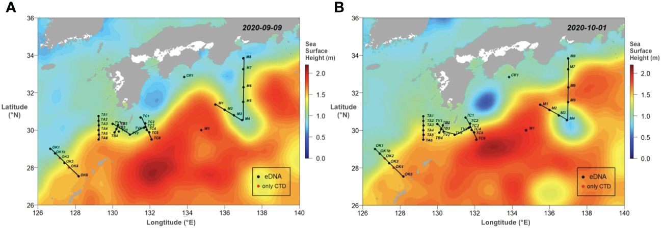
Figure 1 The sea surface topograms capturing the movement of Kuroshio current between 9 September (A) to 1 October 2020 (B). The topograms were colored in sea surface height (m). The black dots were stations with eDNA sampling performed, and the red dots show the ones where only CTD measurements were conducted. Lines connected each sampling transect.

At each station, Conductivity-Temperature-Depth (CTD) system (Sea-Bird Electronics 911plus CTD) was deployed to collect hydrographic data. Water samples were collected with Niskin-X bottles (General Oceanics, USA) equipped on a CTD-carousel system from 10 m, 30 m, 40 m, 50 m, 60 m, 80 m, 100 m, 125 m, 150 m, 200 m, 300 m, 400 m, 600 m, 800 m, and 1,000 m or at 50 m above seafloor if the depth is shallower than 1,000 m. Underwater light penetration was measured at daytime sampling stations once per day by deploying the radiometer PRR-800 with the radiometer PRR-810 on deck (Biospherical Instruments Inc.) to determine the depth of euphotic zone (EZ; 1% irradiance level relative to sea surface). To examine nitrate (NO₃⁻), nitrite (NO₂⁻), ammonium (NH₄⁺), and phosphate (PO₄³⁺) concentrations, water collected in Niskin-X bottles was transferred to 12-mL polycarbonate tubes in duplicate and stored in gastight aluminum bags at −30°C until measuring. Water samples for measuring chlorophyll-a (Chl-a) concentration were collected down to 200 m. For metabarcoding analysis, water samples (~10 L) were collected at 10 m, 50 m, 100 m, and 150 m of all stations except Sta. OK2 and OK4 and filtered through a Sterivex filter (0.45 μm, Millipore SVHV010RS, Merck, Tokyo, Japan). Once the filtration was completed, 2 mL of RNAlater was added into each Sterivex cartridge and stored in a deep freezer at −70°C until DNA extraction.

Ocean Data View 5.5.2 was used to create the map of the studying area, temperature-salinity (TS) diagrams. The vertical profiles of nutrients and Chl-a were created using ggplot2 3.3.5 package in R (Wickham, 2016). If a nutrient concentration was below its detection limit, zero was assigned. The potential density anomaly was calculated in the Ocean Data View 5.5.2. The mixed layer depth (MLD) was defined as where the potential density anomaly is 0.125 kg m⁻³ greater than the surface.

2.2 DNA sample collection and processing

Right before DNA extraction, each Sterivex filter was thawed on ice, and RNAlater inside was removed by aspiration. DNA was extracted following the method in Wong et al. (2020) using a Qiagen DNeasy Blood and Tissue DNA extraction kit. The eluate was stored at −25°C. DNA of four dinoflagellate cultures isolated during the expedition and growing in 1/10 x Daigo’s IMK medium was extracted following the same procedure to create a positive control.

Intended to cover as much dinoflagellate species as possible, universal primer sets TAReuk454FWD1 and TAReukREV3 (Stoeck et al., 2010) and 1389F and 1510R (Amaral-Zettler et al., 2009) were used to amplify the hypervariable V4 and V9 regions of eukaryotic 18S rDNA of extracted DNA samples, respectively (Supplementary Table 4). A two-step PCR was performed using 15 μL of PCR systems with 10 ng to 30 ng of DNA, 0.45 μL of forward and reverse primers (10 μM), Toyobo KOD -Plus- ver. 2 enzyme and reagents from Toyobo KOD -Plus- ver. 2 kit (Toyobo, Japan). The first step amplified the desired regions with the Illumina Paired-End adapters attached, started with an initial activation at 94°C for 2 min, followed by 30 cycles of 10 s at 98°C, 30 s at 56°C, and 60 s at 68°C, and ended at 68°C for 7 min. The second step added indexes allowing sample multiplexing in one Illumina MiSeq run, starting at 94°C for 2 min, followed by eight cycles of 10 s at 98°C, 30 s at 59°C, and 60 s at 68°C, and then final elongation at 68°C for 7 min. Negative controls without the addition of DNA and one positive control (only V4 region amplified) were made. Products of each PCR step were checked on electrophoresis gels.

The PCR products were pooled by adding 100 ng of PCR products of each sample and controls. Because the concentration of the V4 negative control was too low, only the culture mix was pooled. The pooled samples were sent to the commercial sequencing company FASMAC (Atsugi, Japan) and run separately on the Illumina MiSeq platform. The pooled V4 sample was run on one lane of a pair-end 2× 300-bp sequencing run, and the pooled V9 sample was run on a lane of a pair-end 2× 250-bp sequencing run.

2.3 Nutrient and Chl-a measurements

The concentrations of NO₃⁻, NO₂⁻ NH₄⁺ and PO₄³⁺ were measured using absorption spectrophotometry (Strickland and Parsons, 1972) adapted for an auto-analyzer (QuAAtro, BL-Tec). The detection limits for NO₃⁻, NO₂⁻, NH₄⁺, and PO₄³⁺ were 0.05 μM, 0.07 μM, 0.05 μM, and 0.01 μM, respectively. Chl-a samples were filtered on board through Whatman GF/F filters under low vacuum pressure (<0.02 MPa). The filters were soaked in 5 mL of N,N-dimethylformamide and stored at −20°C in dark for 24 h for extracting pigment (Suzuki and Ishimaru, 1990). Chl-a concentration was then measured with a Turner Designs fluorometer on board following a non-acidification method (Welschmeyer, 1994).

2.4 Metabarcoding data processing and taxonomic identification

The raw sequence data (refer to the Data availability statement section) were processed to generate absolute sequence variant (ASV) table of amplified eukaryotic V4 and V9 regions using the DADA2 1.20.0 package in R Studio based on the standard procedure (Callahan et al., 2016). The quality profiles of reads were checked using FASTQC prior to trimming (Andrews, 2010). Taxonomic assignation of generated ASVs was performed using the default setting of function “assignTaxonomy” in DADA2 against the DADA2 trained Protist Ribosomal Reference (PR²) database ver. 4.14.0 (Guillou et al., 2013) that includes a curated 18S rDNA reference database of dinoflagellate (Mordret et al., 2018). The output data comprising of ASV tables and taxonomic annotation were merged with environmental data of sampling stations and directly input to Phyloseq 1.36.0 package in R Studio (McMurdie and Holmes, 2013). The ASV tables were first cleaned by excluding these detected in the negative control, which could be contamination during the experiment. Then, only ASVs belonged to the phylum Dinoflagellata were extracted to form new ASV tables. The new tables were again cleaned by excluding ASVs annotated as symbiotic and parasitic dinoflagellates (Supplementary Table 1). Read depth was standardized to median read depth of samples in Phyloseq, and data artifacts (ASV with a total read count < 0.1% of the sample sum) were excluded from the standardized ASV tables. The ASV will be referred as metabarcodes hereinafter.

For analyzing the relation between species and environmental variables, read counts of metabarcodes assigned to the same taxon at the species level were merged to create a new species read count table using tax_glom command in Phyloseq. The trophic strategy of species detected in both V4 and V9 metabarcodes were assigned on the basis of published literatures and databases (refer to Supplementary Table 2). For simplification, MTD is defined as plastid-containing species with observed predation behavior or food vacuoles in this study.

2.5 Multivariate analysis and visualization

Relative abundance of metabarcodes was calculated as a Phyloseq object using “transform_sample_counts” function or directly in R Studio. To visualize the relative abundances, the values were log10-transformed for plotting heatmaps of species detected by both V4 and V9. Where the relative abundance was zero, 0.01 was assigned. Metabarcode α-diversity indices and Pielou’s evenness index were calculated using Vegan 2.5–7 package in RStudio (Oksanen et al., 2020). Analysis of variance (ANOVA) test was performed followed by Tukey multiple comparisons of means to understand the difference in metabarcode diversity between groups.

Prior to the multivariate analysis, standardized read counts of dinoflagellate metabarcodes were Hellinger-transformed in Vegan. Then, Bray-Curtis–based non-metric multidimensional scaling (NMDS) was calculated using Vegan to examine regional dissimilarity, and detrended correspondence analysis (DCA) was used to explore the correlation between the diversity of dinoflagellate communities and environmental variables in Vegan, as a unimodal fit was expected. Once significant variables identified by p-value, the relation between these variables and the distribution of species annotated in both V4 and V9 was analyzed by canonical correlation analysis (CCA) in Vegan. From species read count table, a species occurrence data was constructed by assigning 1 (present) or 0 (absent) to each species annotated. To assess niche of each species in the study area, we applied an Outlying Mean Index (OMI) analysis using the Subniche 1.5 package in R, which is based on the occurrence data and PCA results of environmental condition (Dolé Dec et al., 2000; Karasiewicz et al., 2017). The OMI is the index of marginality that measures the distance between the average habitat conditions of one species and the average conditions of the whole sampling region. Here, OMI would be used to relate the distribution to the sampling station categories. To know the preferred habitats of each species, the coordinates on the first two factorial axes were plotted with the polygons of environmental spaces based on PCA analysis. The above analysis was visualized using ggplot2 3.3.5 package in R (Wickham, 2016).

3 Results

3.1 Environmental characteristics of the study area

It has been well demonstrated that the Kuroshio took bimodal paths off southern coast of Honshu, Japan (Kawabe, 1995). The Kuroshio flows easterly along the continental shelf approximated to 33°N, but the path left the coast and directed to the south approximated to 30°N and then returned to the north, forming a large meander path (LMP) (Figure 1A). When the expedition started, the LMP was observed off Honshu around 137°E, and the southern edge reached to 29°30̬′N (Figure 1A; Supplementary Video 1). At where the path met the M transect (Sta. M1 to M8), it started extending southward from 14 September and finally separated from the Kuroshio axis around 28 September. As a result, a cyclonic eddy was formed (Figure 1B). The sampling along the M transect started from 30 September after the formation of the cyclonic eddy. We set Sta. M4 at the center of the eddy.

Water property in the study area exhibited subtropic water features of high temperature and salinity, having surface water temperature above 26°C and salinity over 34 (Figure 2). Based on the indicator temperature of the Kuroshio axis at 200 m (Kawabe, 2003), which is 17°C in the ECS, 16°C in the east of the Kyushu, and 15°C in the south of the Honshu, most stations were positioned on the Kuroshio axis or the south of the axis. The exceptions were some stations on the continental shelf and inside the cyclonic eddy (Sta. M3 and M4) at which low salinity (<34.0) was observed. It was apparent that the water in the eddy was transported from coast, as the water property of Sta. M3 and M4 resembled it of Coastal stations, being colder and less saline comparing to other stations along the transect M (Figure 2). From the water properties and formation of the cyclonic eddy, we grouped sampling stations into three categories: Coastal stations (Sta. OK1, OK1b, TA1, and TC1) characterized by cooler and less saline water, Eddy stations inside the eddy (Sta. M3 and M4) with similar water property to Coastal stations, and KC stations on the axis and south with warm and high salinity water (Table 1). The mixed layer depth determined by a difference of 0.125 σθ respect to the sea surface was shallow at Coastal stations (21.2 ± 14.8 m) compared with one in the KC station (46.3 ± 14.3 m) (Table 2). At Eddy stations, the bottom of mixed layer shoaled to 40 m at Sta. M3 and 28 m at Sta. M4, showing an uplift of subsurface water in the cyclonic eddy. The depth of euphotic zone (EZ) was from 32 m to 107 m (Table 3). The shallowest was observed at coastal Sta. OK1 (32 m), followed by Eddy station M4 (56 m) and Coastal station TA1 (69 m). All the EZ of KC stations examined (range from 76 m to 107 m; mean ± SD, 92.1 ± 10.0 m) were deeper than those in the Coastal and Eddy stations.

Figure 2

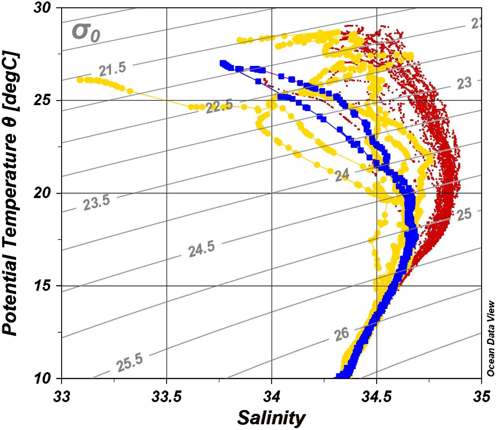
Figure 2 The potential temperature-salinity (T-S) diagram of all stations colored by station category. Each dot represents a measuring point. Blue, Eddy stations; yellow, Coastal stations; red, KC stations.

Table 1

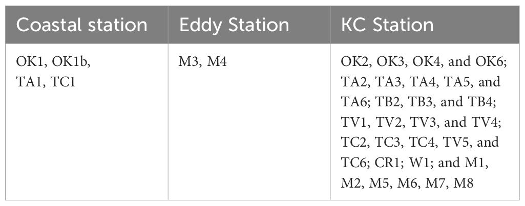
Table 1 Categories of sampling stations.

Table 2

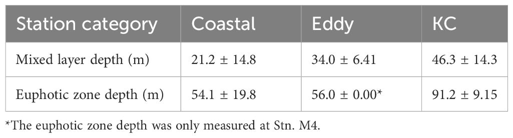
Table 2 The average mixed layer depth and euphotic zone depth of each station category.

Table 3

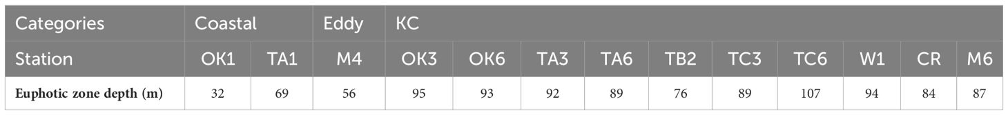
Table 3 The depth of 1% light depth relative to surface irradiance (the euphotic zone depth), measured once per day.

Nutrients such as NO₃⁻, NO₂⁻ and PO₄³⁺ were depleted in EZ and increasing with depth (Figure 3; Supplementary Data Sheet 1). Concentration of NH₄⁺ was below the detection limit at most stations throughout. Exceptions were stations at shallower shelf regions and inside the cyclonic eddy, where higher nutrient concentrations were observed in the EZ. The depth of Chl-a maximum was generally observed between 50 m and 100 m, except Coastal stations where it was above 50 m.

Figure 3

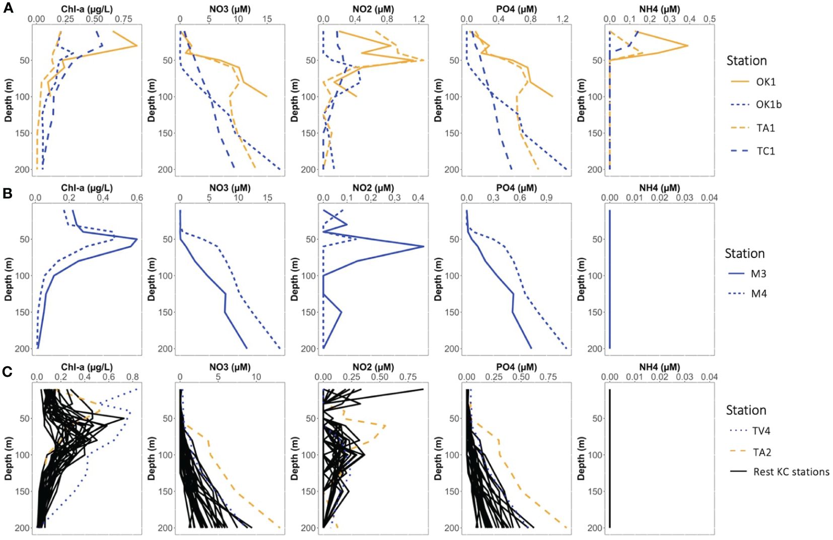
Figure 3 The vertical profiles of chlorophyl-a and nutrient (nitrate, nitrite, phosphate, and ammonium) concentrations at (A) Coastal stations, (B) Eddy stations, and (C) KC stations.

3.2 Dinoflagellate metabarcodes

A total of 15,491 V4 and 17,963 V9 metabarcodes were generated by DADA2 from a total of 7,311,304 and 9,300,530 reads. After matching against the PR² database and filtering out data artifacts, 7,269 V4 and 5,110 V9 metabarcodes were annotated under the phylum Dinoflagellata. Both regions detected a high genetic diversity of parasitic Syndiniales, which accounted 62% V4 and 32% V9 dinoflagellate metabarcodes. The most abundant orders of Syndiniales were Dino-Group-I and Group-II (Supplementary Figure 1). After filtering out metabarcodes of Syndiniales and other symbiotic or parasitic taxa (Supplementary Table 1), 2,702 V4 and 3,402 V9 metabarcodes remained. Once the read depth was standardized, metabarcodes of less than 0.1% relative abundance was removed, and 1,571 V4 and 2,800 V9 metabarcodes remained. An average of 122.41 ± 49.57 metabarcodes per sample present in the V4 dataset and 170.98 ± 56.01 metabarcodes per sample in the V9 dataset. Among these, 610 V4 and 274 V9 metabarcodes were annotated to 47 and 41 genera under eight orders, respectively. The taxa ended with one or more X such as the order Dinophyceae_X and Dinophyta_XX contained unknown Dinoflagellate sequences detected by contributors of PR² database, mostly from environmental samples. The most frequently detected order was Gymnodiniales, followed by Peridiniales (Figure 4), and the most frequently detected genera were Gyrodinium, Karlodinium, Gymnodinium, Lepidodinium, and Tripos. Aligning results from V4 and V9 regions, a total of 30 dinoflagellate species were detected (Figure 5; Supplementary Table 2). Most species occurred at the KC stations, and Gyrodinium fusiforme and Karlodinium veneficum prevailed at all stations. The average relative abundance of unknown V9 metabarcodes was 48.53 ± 12.97%, larger than it observed in the V4 region (25.57 ± 5.10%).

Figure 4

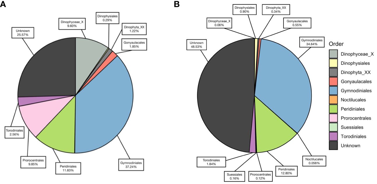
Figure 4 The percentage of each dinoflagellate order annotated against PR² database, using (A) V4 metabarcodes and (B) V9 metabarcodes.

Figure 5

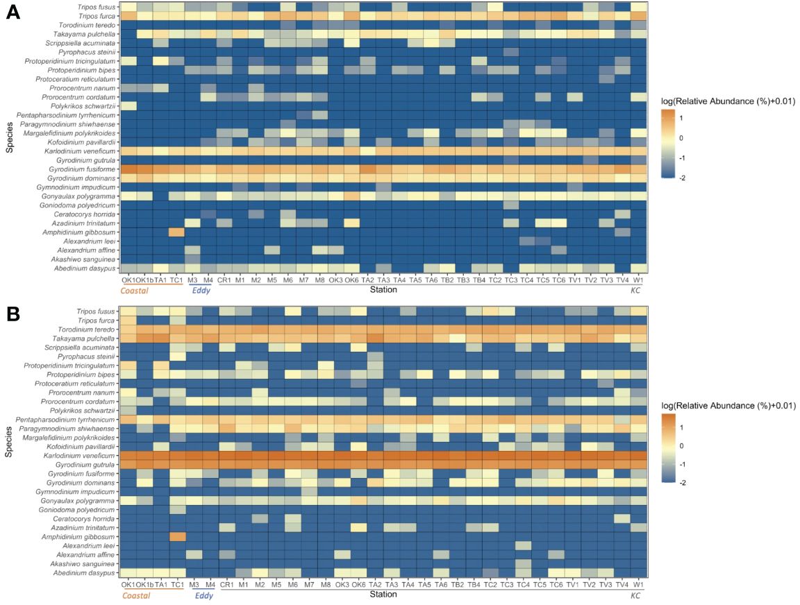
Figure 5 Log10-transformed relative abundances of the 30 species detected by both (A) V4 and (B) V9. The order of stations moves from Coastal, Eddy to KC stations.

Because many V4 and V9 dinoflagellate metabarcodes could not be annotated to lower taxonomic levels, the genetic diversity that was assessed by Shannon diversity and Pielou’s evenness indices was calculated on the basis of the number of metabarcodes and standardized read counts of metabarcodes. While a general high genetic diversity and evenness were observed, the mean value of Shannon index of V4 metabarcodes (4.04) was significantly lower than one of V9 (4.66), as well as the means of Pielou’s evenness index (0.856 for V4 and 0.915 for V9 metabarcodes). The differences among depths and categories were illustrated on Figure 6. Whereas Shannon diversity of V4 metabarcodes decreased with depth, that of V9 metabarcodes remained unchanged due to increasing evenness. Communities at Coastal and Eddy stations at 150 m were generally less diverse and even compared with KC stations. The ANOVA test verified the significant differences in genetic diversities among depths and station categories (p < 0.001, Table 4). The Tukey test showed that the differences were attributed to communities from surface (10 m and 50 m) and subsurface (100 m and 150 m), as well as from KC and Coastal stations (Supplementary Table 3).

Figure 6

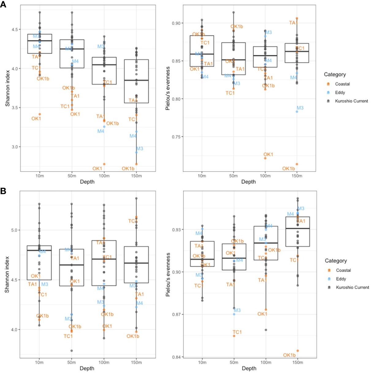
Figure 6 Shannon diversity index and Pielou’s evenness index of dinoflagellate communities constructed on (A) V4 metabarcodes and (B) V9 metabarcodes. Each dot represents a community from a sampling depth at station and is colored by station category. Only communities at Eddy and Coastal stations are annotated.

Table 4

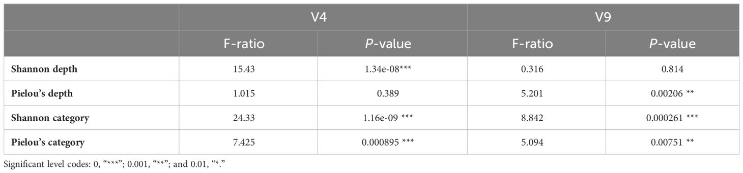
Table 4 ANOVA tests to compare Shannon and Pielou’s indices between different sampling depth and station categories.

3.3 Community structure of dinoflagellate and its control factors

Metabarcode compositions of dinoflagellates between samples were compared by NMDS analysis (Figure 7). Surface communities from 10 m to 50 m were highly similar with each other especially at the KC stations, and the exceptions were Coastal stations like Sta. OK1 and TA1. Subsurface communities at 100 m and 150 m were distanced from the surface communities and from each other, and their compositions varied noticeably more with depth, especially between station categories. These agreed the results of ANOVA and Tukey tests (Table 4; Supplementary Table 3). Although facing alike environmental conditions, the subsurface communities at Coastal stations OK1, OK1b, and TA1 were similar between the Eddy stations, and the communities from subsurface layers (100 m and 150 m) of Sta. TC1 resembled to communities at KC stations.

Figure 7

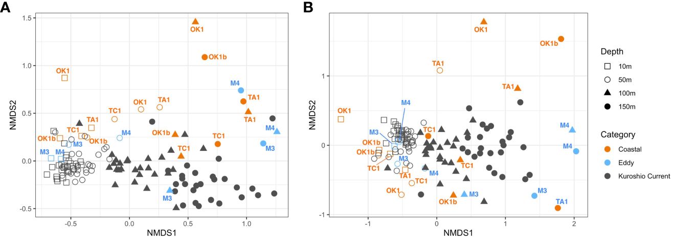
Figure 7 Non-metric multidimensional scaling (NMDS) plots showing the dissimilarity in (A) V4 and (B) V9 dinoflagellate communities. Each dot represents a community from a sampling depth at station. It is shaped according to its sampling depth and colored based on station category. Only communities at Eddy and Coastal stations are annotated.

To explore the dinoflagellate community structure and the influence of environmental factors, DCA analysis was conducted on the basis of metabarcodes and their read counts at each station (Figure 8). Major differences in communities could be related to temperature and sampling depth, which was exhibited along the axis of DCA1, separating communities of different sampling depth. Surface communities of 10 m and 50 m again formed a tighter group comparing with subsurface communities of 100 m and 150 m, excepting those at Coastal stations. Coastal stations demonstrated their distinct community structures from KC stations along the axis of DCA2, which could be correlated to the higher nutrient concentrations at these stations. Among all environmental variables, NH₄⁺ was not significant by both V4 and V9 and NO₂⁻ was the least significant factor in DCA analysis of V4 datasets.

Figure 8

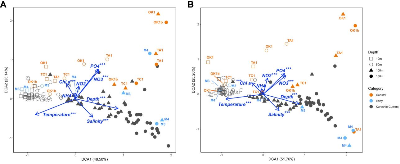
Figure 8 Detrended correspondence analysis (DCA) plots of (A) V4 and (B) V9 dinoflagellate communities, demonstrating the correlation between environmental variables (plotted as blue vectors) and communities at a sampling depth of a station (dots). Each dot is shaped according to its sampling depth and colored by the station category. Only communities at Eddy and Coastal stations are annotated.

3.4 Trophic strategies of dinoflagellate species

To further explore the relationship between dinoflagellate species and environmental factors, metabarcodes of dinoflagellate species detected by both V4 and V9 regions were extracted along with the numbers of read counts and the trophic strategy of each species (Supplementary Data Sheet 1). Each species annotated present at an average of 13.23 ± 12.04 and 14.33 ± 12.50 stations based on V4 and V9 metabarcodes. Out of the 30 dinoflagellate species, nine are autotrophy (ATD), eight are heterotrophy (HTD), and 13 are mixotrophy (MTD).

The environmental variables proven to be significant (p < 0.001) by the DCA analysis were chosen for the constrained CCA analysis (Figures 9A, B). The correlation illustrated by V4 and V9 metabarcodes approximately agreed with each other. Over half of the 30 species were more correlated to warmer water, and they were more likely to appear and being abundant at the surface oligotrophic habitats. The abundance of most MTD species was also related to the oligotrophic and warm euphotic surface habitats. For ATDs, they tended to appear at warmer surface, although this trend was not that obvious in community structures of V9 metabarcodes. Appearance of HTDs was more corresponding to higher nutrient levels and lower Chl a concentration. Rare species were situated relatively far from the environmental vectors on the CCA plots. For example, Polykrikos schwartzii (MTD), which was the farmost species on both CCA plots along the CCA2 axis, only present at the surface of Sta. OK1 and OK1b (Figures 5, 9).

Figure 9

Figure 9 Canonical correspondence analysis (CCA) plots showing the correlation between environmental variables (plotted as blue vectors) and species distribution calculated from (A) V4 and (B) V9 metabarcodes. Each species is colored according to its trophic strategy and annotated by its name abbreviation (refer to Supplementary Table 2).

The realized niche of each species was plotted against the realized environmental space by each category and sampling depth. On the plots (Figure 10), the origin of the OMI ordination represents the average habitat condition, which resembles the environment of the KC stations at 100 m with moderate levels of all nutrients, temperature, and salinity in our data set. The space of Coastal stations was boarder due to great environmental variance among Coastal stations, such as the lower NO₃⁻ and PO₄³⁻ concentrations at Sta. OK1b and TV1 comparing to Sta. OK1 and TA1 above 150 m (Figure 3). The area of Eddy stations was mostly within Coastal stations due to similarly low salinity and higher nutrient levels.

Figure 10

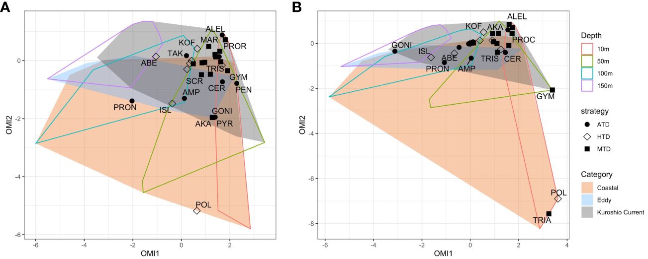
Figure 10 Outlying mean index (OMI) analysis plots showing the realized niche of dinoflagellate species on the realized environmental spaces (minimum convex polygons) calculated on (A) V4 and (B) V9 metabarcodes. Each species is shaped according to its trophic strategy. The contour of realized environment space is plotted as depth (outlined polygons) and station category (colored polygons).

Most species could be found within 10 m and 50 m of KC and Eddy stations and approximated to the average habitat condition. Within KC stations, the realized niche of species having same trophic strategy was generally closer. When moving into the Coastal and Eddy habitats on OMI plots, the realized niche of species became more distanced. Most MTDs were detected within 10 m and 50 m and had adjacent niche. Comparing to MTDs, a few ATDs were detected below 100 m, and HTDs lived below 50 m in general. The exception was Polykrikos schwartzii (HTD), which only appeared at 10 m of Sta. OK1 and OK1b; thus, its realized niche was at the edge of Coastal stations (Figures 5, 10). Because the occurrence of some species was different in V4 and V9 metabarcodes, the realized niches of these species determined by V4 and V9 were different consequently. Tripos furca is a cosmopolitan species and was detected at almost every station in V4 metabarcodes, but it was only present at 10 m of Sta. OK1 and TC1 in V9 metabarcodes (Figure 5).

3.5 Distribution of HAB species

A total of 15 HAB species was detected by V4 but only nine of them were detected by V9 (Supplementary Data Sheet 2). Most HAB species annotated present at KC and Eddy stations. Gonyaulax polygramma, Karlodinium veneficum, and Takayama pulchella, all associated to fish killing, appeared at almost every station by both of the V4 and V9 (Figure 5).

Distribution of most HAB species was correlated to warmer surface habitats at 10 m and 50 m, and only two HAB species correlated to subsurface (Figure 10). One was Takayama pulchella having a maximum relative abundance approximate to nutriclines of most KC stations, which were generally below 50 m (Figures 3, 5). The other was Amphidinium gibbosum that also had a realized niche between 50 m and 100 m. Some infrequent species only appeared at Eddy or KC stations, except the benthic species Amphidinium gibbosum (Murray et al., 2004) which only occurred at 50 m of Sta. TC1 and 100 m of Sta. TV4 (Figures 3, 5, 10).

The relative abundances of HAB assemblages were not significantly greater at Coastal or Eddy stations comparing with KC stations (Table 5). A lower number of HAB species were detected at those stations. No HAB species’ realized niche was solely correlated to the coastal environment by OMI analysis, and only the presence of few species, Gonyaulax polygramma, Karlodinium veneficum, and Takayama pulchella, at Coastal stations was confirmed by both V4 and V9. Margalefidinium (= Cochlodinium) polykrikoides, one of the reoccurring red tide species along Japan coast (Iwataki et al., 2008; Furuya et al., 2018), was not detected at Coastal stations (Figure 5).

Table 5

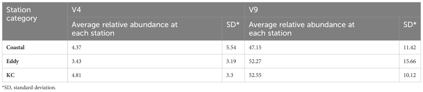
Table 5 The average relative abundance of dinoflagellate HAB assemblages of each station category.

4 Discussion

4.1 Environmental conditions

From the year of 2017, the offshore LMP had been observed till the beginning of the cruise (Sugimoto et al., 2021) (Figure 1A). Our sampling stations originally intended to cover several transects of the Kuroshio axis along the LMP from the ECS off Okinawa to the south of Honshu, Japan and offshore region south of the axis, including regions onshore and offshore. While moving onshore, a cold eddy was formed and separated from the Kuroshio axis (Figure 1B). This change in path greatly influences local marine environment, biogeography, and productivity in the area (Nakata and Hidaka, 2003).

Three station categories—Coastal, KC, and Eddy—were established as they were influenced by Kuroshio differently. All KC stations exhibited typical Kuroshio characteristics of warm and saline surface water. The water property of Coastal stations was influenced by the cold and less saline coastal water, especially above 200 m, and active mixing at Coastal stations was observed by irregular temperature and salinity. The unforeseen change of LMP brought great impact onshore, and some onshore stations such as Sta. CR1 and M8 were identified as KC stations, demonstrating that the influence of Kuroshio Current was more than its path displayed on the ocean surface topography (Figure 1). The TS diagrams of Eddy stations were similar to that of Coastal stations and distinct from that of the KC stations (Figure 2). At the center of the eddy (Sta. M4), the thermocline and halocline were observed at 29 m, suggesting that the original coastal water property and dinoflagellate community were kept inside the eddy.

The distinction among environmental characteristics of the three station categories was the nutrient concentration above 50 m (Figure 3). At Kuroshio stations, the nutriclines were generally observed around 60 m to 100 m and nutrients were depleted above the nutricline, except these at the Tokara strait (e.g., Sta. TA2 and TC1) where strong turbulent mixing due to the shallow depth and sea mounts supplied nutrients to the surface (Nagai et al., 2021). At Coastal stations, nutriclines generally located at layers shallower than 50 m, and higher nutrient concentrations were observed at sea surface. Coastal stations were especially rich in NH₄⁺, whereas its concentration was below the detection limit (0.05 μM) at KC and Eddy stations. Similarly, the nutriclines were observed in layer shallower than 50 m in the eddy, and the NO₃⁻ and PO₄³⁺ concentrations at 50 m of Sta. M4 (3.91 and 0.30 μM, respectively) were similar to those at 100 m of the KC stations. As cyclonic eddy induces upwelling (Bibby et al., 2008; Uchiyama et al., 2017), this eddy may replenish nutrients from the uplifted thermocline. However, the uplift of thermocline and nutriclines did not reach to 10 m, and nutrients were depleted at 10 m in the eddy.

4.2 Community compositions influenced by environmental variables

Dinoflagellate community compositions were localized horizontally and vertically in the study area regardless the station categories, and the dissimilarity was correlated greatly to sampling depth and nutrient levels (Figures 7, 8). Depth is the vital factor that corresponded to vertical temperature change and light gradient, separating communities of different sampling depth. The nutrient levels caused the variance of communities of different station categories, especially below 50 m. The formation of the tight group of surface KC and Eddy communities may be related to the well-mixed surface layers of the current, and the relatively stratified subsurface layers differentiated the subsurface communities. The vertical separation among surface and subsurface communities also appeared on the profiles of Shannon and Pielous’s indices, proven by the Turkey Test (Supplementary Table 3). Similar vertical stratification of dinoflagellate and protist assemblages was observed in other ecosystems (Schnetzer et al., 2011; Cohen et al., 2021; Ollison et al., 2021; Carve et al., 2024). Carve et al. (2024) also mentioned that the wind-induced vertical mixing could lead to highly similar assemblages in the mixed surface layer. Irradiance could be another factor because, at 100 m of KC stations, it was being approximately 1% relative to surface, suggesting possible existence of autotrophy at this depth. However, the irradiance at 150 m of every station was too dim to support photosynthesis.

The levels of Chl-a and nutrients were mainly correlated to the separation of nutrient-rich Coastal stations from KC stations. At Eddy stations, the surface communities resembled the surface KC communities (Figures 7, 8) despite their similar water property to Coastal stations, suggesting potential influence of the water from Kuroshio axis. Below 100 m, the Eddy communities were similar to those at Coastal stations because the eddy trapped coastal water inside.

The dissimilarity among communities represents the variation in genetic diversity and evenness between communities. The diversity and evenness indices were generally higher at KC stations relative to Coastal and Eddy stations because more minor metabarcodes present at these stations (Figure 6). Once metabarcodes were grouped by taxa, fewer taxa were observed at Coastal stations such as Sta. TA1. The ubiquitous species among the 30 species annotated demonstrated no preference to Coastal stations. A few rare species were specialized to local environment by their greater relative abundance at some Coastal stations. The most conspicuous example was Amphidinium gibbosum (ATD) whose only presence was relatively abundant at Sta. TC1 (Figure 5). Others such as Abedinium dasypus and Protoperidinium tricingulatum, both HTDs that only present below 100 m in this study, were rare in the sampling area but slightly more abundant at Sta. TA1. It indicates a possible advantage that these species possessed in nutrient-rich environment. However, the physiology of rare species was hardly studies due to difficulties in sampling, identifying, and culturing, stressing the necessity of such knowledge in understanding their relation to environment.

Within communities, the environmental adaptation of the species detected was analyzed by means of OMI analysis. Despite the drawn polygon of Coastal stations appeared to contain other station categories, its broadness was due to the different environment in ECS and Tokara strait. Most species were found in the warm surface habitat of the KC and Eddy stations. A few species were shown to be specialized for deeper habitats such as Prorocentrum nanum (ATD) and Abedinium dasypus (HTD).

Most species annotated were photosynthetic ATD and MTD, and their correlation with shallower warm water was expected as a higher level of irradiance is required for photosynthesis. Most ATDs’ distribution correlated to temperature and had realized niches at 50 m. Alexandrium leei and Azadinium trinitatum are the examples. However, more MTDs were detected at 10 m than ATDs and appeared to be specialized for surface water, and the realized niche of MTDs was more aggregated compared to ATDs. Photoacclimation by adjusting Chl:C ratio is required to optimize photosynthesis and prevent photodamage, and nutrient limitation in surface water (above 10 m) could restrain the repairing ability of phytoplankton under strong irradiance (Litchman et al., 2002; Li et al., 2021). Phagotrophy could potentially help MTDs acquiring carbon without elevating Chl:C and adapting higher irradiance (Mitra et al., 2023). For MTDs possessing diverse prey types and varied surviving strategies regarding light and nutrient conditions (Hansen, 2011), it is possible that they occupied more adjacent realized niches in a habitat. Considering their abundance in the water column above 50 m, our results indicated a more complex and dynamic food web and support the hypothesis of MTDs enhancing trophic transfer efficiency (Flynn and Mitra, 2009; Ward and Follows, 2016; Stoecker et al., 2017). However, more in situ and laboratory experiments on their physiology and interaction with other protists are necessary to elucidate their roles in the food web.

Nonetheless, few rare ATDs were detected at deeper layers, such as the dinoflagellate Prorocentrum nanum, which had a realized niche at 100 m (Figure 10). Because photosynthesis was almost impossible under 100 m, they could be either be cysts, an aggregate, or attach on macroalgae then sink below 100 m. It is disputable that they could possess unique physiology traits to survive in low light conditions unless they possess undiscovered mixotrophic ability, which helps them survive in the dark (Cohen et al., 2021).

The realized niche of HTDs varied largely among species. For example, of the two HTD species, Protoperidinium tricingulatum and Protoperidinium bipes, it was correlated to different environment variables. The first species often detected at 50 m and was more abundant at Coastal stations (Schneider et al., 2020). The other species was closely correlated to temperature because of its frequent appearance at 10 m and 50 m of oligotrophic KC and Eddy stations. However, when a species was rare and only detected at a few stations, its correlation with these environment variables is statistically unexplainable, hence locating far from the vectors.

4.3 Varying resolution preference but similar trend between V4 and V9 metabarcodes

The hypervariable V4 and V9 regions of the 18S rRNA are widely used DNA markers in marine protist research (Pawlowski et al., 2012; Burki et al., 2021). In this study, both regions exhibited their competence and arrived at similar statistical results based on community structures and environmental impacts. The V4 region showed more potent resolution power, possibly owing to its more completed dinoflagellate library and longer fragment size. The occurrence of most species was similar, as well as the tendency of their relative abundance in the sampling site; thus, similar pattern could be obtained. Karlodinium veneficum was such an example where coherent conclusion could be drawn despite subtle variations. However, huge variance was also observed in the relative abundance of some species. For example, G. gutrula was pervasive and also the second dominant species annotated by V9, but it appeared as a rare species among V4 metabarcodes. T. furca was the opposite, which being common based on V4 metabarcodes but rare in the V9 data set. Their correlations to environmental variables and realized niches based on V4 and V9 were distinct from each other.

The divergence in the read counts of metabarcodes depicts dinoflagellate community differently at certain stations. At the Eddy stations, their distant subsurface communities were positively correlated to nutrient concentrations on DCA plot based on V4 metabarcodes, but this correlation was lost on it built by V9 metabarcodes (Figure 8). These differences could lead to separate interpretation if sole barcode region is used in a study and create uncertainty in comparison with other literature. The reason of it could be generalized down to the different resolution power and the genetic databases of the two. Based on the study by Ki (2012), the hypervariable V2–V4 has the best discriminative ability as the fragment size of V9 may be too short. In addition, the V4 regions detected more Prorocentrales and Syndiniales metabarcodes comparing to V9, and V9 detected more diversity in other subgroups like Peridiniales in our datasets. Similar observation also appeared in other studies (Stoeck et al., 2010; An et al., 2020; Choi and Park, 2020). It could be due to unintended preferential detection of primer sets or over-representation during amplification (Stoeck et al., 2010; An et al., 2020). Nevertheless, nearly half of the V4 and three quarters of the V9 metabarcodes could not be annotated to species level, and the relative abundance of species derived from V4 and V9 metabarcodes differed (Figures 4, 5). The present results based on existing genetic databases of dinoflagellate indicated the need of further efforts to improve the resolution to species level and complete dinoflagellate genetic database.

4.4 Kuroshio current as a potential introducer of HAB species

Although many HAB species were pervasive and found in all stations (e.g., Gonyaulax polygramma, Takayama pulchella, and Karlodinium veneficum), the number of taxa and the relative abundance of HAB assemblages were greater at KC stations and less at Coastal stations (Supplementary File 2). These HAB species may have advantage in surviving oligotrophic environments, but non-HAB species also have the potential to surpass some cosmopolitan HAB species along coasts. Alexandrium leei, ATD that had caused HAB in coasts of Japan, is present infrequently at 10 m with low relative abundance; whereas Gyrodinium fusiforme, a HTD species feeding on dinoflagellate, diatom, haptophytes, and cryptophytes, was more abundant at Coastal stations (Naustvoll, 2000). This feeding strategy of G. fusiforme might help it to thrive at coastal environments where more preys live. At the same time, the high surface water temperature during this period may not favor Alexandrium leei because its optimal growth temperature was 20°C (Shikata et al., 2020). In our data, no HAB species solely presented at Coastal nor Eddy stations, except Amphidinium gibbosum that could either be brought up with bottom sediments or being endosymbionts of others (Murray et al., 2004).

Majority of the HAB species detected were absent at Coastal stations, such as Margalefidinium polykrikoides (MTD), indicating that Kuroshio could introduce HAB species to coastal regions and signifies the role of oceanic circulation that plays in the mechanism of HAB in addition to anthropogenic factors. M. polykrikoides has caused HAB first in East Asia, and its blooms spread globally after 1990. Studies have shown the outbreaks of this species were transported by currents from Korean coastal water to the southwest Sea of Japan and from the northern of Borneo, Malaysia to Palawan, Philippines, monitored using satellite image (Azanza et al., 2008; Onitsuka et al., 2010). Another study by Sildever et al. (2019) also monitored dispersal of this species along Hokkaido coasts by Soya warm current (a continuation of Tsushima Warm Current, a branch of Kuroshio). The molecular phylogenetic data also confirmed the differences in ribotypes in Asian coasts; American ribotype in Sabah, Malaysia, and Lampung, Indonesia; Philippine ribotype in the Philippines; and East Asian ribotype in Hong Kong, Japan, and Korea (Iwataki et al., 2007, 2008; Thoha et al., 2019). By performing LSU rDNA–based qPCR, a study conducted in Korean coastline and Tsushima Strait revealed that the Tsushima Warm Current could introduce the Philippine ribotypes into southern Korean water and potentially contributed the M. polykrikoides bloomings in 2009 in southern Korean coast (Park et al., 2018). Meanwhile, the study demonstrated the potential of the LSU rDNA–based metabarcoding analysis in identifying ribotypes of HAB dinoflagellates and elucidating the blooming mechanism. Another study conducted in the Jeju Warm Current, a branch of the Kuroshio Current in the northeastern ECS, also proposed the potential introduction of HAB species into the region by the Kuroshio Current (Kim et al., 2023). Some other HAB species mentioned in this study also present our study, such as Alexandrium affine, Margalefidinium polykrikoides, and Takayama pulchella (Kim et al., 2023). As Kawakami et al. (2023) suggest that the northward movement of Kuroshio greatly warms the surrounding region and may impact local marine biota, the introduction of HAB species along with warming water potentially increases risks of HAB along Japanese coast and prolonging it.

Additionally, the V9 regions may not be the best choice in detecting the bloom-forming dinoflagellate species. Only nine species were identified from V9 metabarcodes comparing to total of 15 species from V4 metabarcodes. The V9 primers may also have strong preference in Karlodinium veneficum, as its relative abundance among V9 metabarcodes was over 30% at all stations.

5 Conclusion

This study successfully illustrated the distribution of the highly diverse dinoflagellate communities in the Kuroshio region from the north of Okinawa to the south of Honshu, including a newly formed cyclonic eddy separated from the Kuroshio. As the Kuroshio LMD shifted its path and formed an eddy, coastal water could be trapped inside it, and three stations categories (Coastal, Eddy and KC) were set according to the influence received from the Kuroshio in hydrography. Dinoflagellate communities of each station category had its own traits. Overall, KC stations carried the highest genetic diversity, the greatest number of taxa, and more HAB species. The variation in dinoflagellate communities reflects the difference in local environments. ATDs and MTDs were dominated in this study, mostly corresponded to the warm surface of KC stations. Comparing to ATDs, the realized niches of MTDs were closer together, suggesting their diverse surviving strategies and a more dynamic food web at the surface. Only the niche of a few ATDs and HTDs were correlated to deeper layers. Most HAB species are ATDs or MTDs and were common in the sampling region, but the stations influenced by the Kuroshio contained more HAB species than the nutrient-rich Coastal stations. It demonstrates the potential role of the Kuroshio carrying HAB species downstream. Our results also clearly stated the difference between the two barcodes as the species and relative abundance from the two hypervariable regions varied despite the similar statistical analysis results. The annotated taxa barely overlapped between the two regions, and both had over a quarter of ASV not annotated to the order level. The problem appeared to be raised from the limitation of current database in addition to the effect of chosen primers.

As the first metabarcoding survey targeting the Kuroshio region, this study highlighted the high diversity in oligotrophic oceanic current and the correlation between dinoflagellate communities and local environment, providing a basic and holistic understanding of the biogeography of dinoflagellate community. For the future dinoflagellate study, sampling efforts in marine species and monitoring their distribution are essential to complete the reference library. The obstacles and limitations of metabarcoding, such as data reproducibility between different barcode regions and bioinformatic processing in the database, are to be overcome. Thus, multiple barcode regions and appropriate bioinformatic method are essential to build a concrete foundation of metabarcoding study. Meanwhile, a consistent monitoring of dinoflagellate using the metabarcoding approach in- and offshore is needed to untangle the mechanism of dispersion and formation of HABs, for reducing or preventing the consequential economic and social impacts by proper anticipation or countermeasure.

Data availability statement

The datasets presented in this study can be found in online repositories. The names of the repository/repositories and accession number(s) can be found below: https://www.ncbi.nlm.nih.gov/, PRJNA1050322; https://www.ncbi.nlm.nih.gov/, PRJNA1049584.

Author contributions

YW: Conceptualization, Data curation, Formal analysis, Investigation, Methodology, Validation, Visualization, Writing – original draft, Writing – review & editing. JH: Formal analysis, Methodology, Validation, Writing – review & editing. FZ: Formal analysis, Methodology, Validation, Visualization, Writing – review & editing. MI: Methodology, Writing – review & editing. SJ: Conceptualization, Data curation, Formal analysis, Visualization, Writing – review & editing. HO: Data curation, Formal Analysis, Methodology, Writing – review & editing. JI: Data curation, Methodology, Writing – review & editing. SH: Data curation, Formal analysis, Methodology, Resources, Writing – review & editing. HS: Conceptualization, Data curation, Formal analysis, Funding acquisition, Investigation, Methodology, Resources, Supervision, Validation, Writing – review & editing.

Funding

The author(s) declare financial support was received for the research, authorship, and/or publication of this article. This study was supported by SKED and funded by MEXT (Grant Number JPMXD0511102330) to HS and by UTokyo FSI project “Ocean DNA” to SH.

Acknowledgments

We would like to thank the captains and crews of the RV Hakuho Maru for their support with the sampling. The research cruise was supported by Cooperative Research Program of Atmosphere and Ocean Research Institute, The University of Tokyo (JURCAOSSH20–17).

Conflict of interest

The authors declare that the research was conducted in the absence of any commercial or financial relationships that could be construed as a potential conflict of interest.

The author(s) declared that they were an editorial board member of Frontiers, at the time of submission. This had no impact on the peer review process and the final decision.

The reviewer HG declared a past co-authorship with the author MI to the handling editor.

Publisher’s note

All claims expressed in this article are solely those of the authors and do not necessarily represent those of their affiliated organizations, or those of the publisher, the editors and the reviewers. Any product that may be evaluated in this article, or claim that may be made by its manufacturer, is not guaranteed or endorsed by the publisher.

Supplementary material

The Supplementary Material for this article can be found online at: https://www.frontiersin.org/articles/10.3389/fmars.2024.1361452/full#supplementary-material

Supplementary Video 1 | A short SSH video demonstrating the movement of Kuroshio large meander and the formation of eddy during the sampling period.

Supplementary Presentation 1 | Supplementary figures and tables.

Supplementary Data Sheet 1 | Sample information including location, hydrographic and nutrient conditions of sample sites.

Supplementary Data Sheet 2 | Relative abundance (%) of all HAB species annotated in V4 and V9 metabarcodes.

Supplementary Data Sheet 3 | Relative abundance (%) of the 30 common species annotated in V4 and V9 metabarcodes at each sampling station.

Supplementary Data Sheet 4 | The coordinate values of NMDS analysis and eigenvalues of DCA analysis by samples.

Supplementary Data Sheet 5 | The coordinate values of the 30 common species annotated in V4 and V9 metabarcodes calculated from CCA and OMI analysis.

References

Amaral-Zettler L. A., McCliment E. A., Ducklow H. W., Huse S. M. (2009). A method for studying protistan diversity using massively parallel sequencing of V9 hypervariable regions of small-subunit ribosomal RNA Genes. PloS One 4 (12). doi: 10.1371/annotation/50c43133-0df5-4b8b-8975-8cc37d4f2f26

CrossRef Full Text | Google Scholar

An J. B., Lee H. B., Woo S. Y., Do H. R., Jeong D. H., Choi J. M., et al. (2020). “Exploring the benthic eukaryotic diversity at a deep-sea hydrothermal vent (Onnuri Vent Field) in the Indian Ocean based on Illumina sequencing,” in Proceedings of the Joint online meeting of the Japan Society of Protistology and Korean Society of Protistologists. Japan Society of Protistology. Available at: https://sciwatch.kiost.ac.kr/handle/2020.kiost/40611.

Google Scholar

Anderson D. M., Cembella A. D., Hallegraeff G. M. (2012). Progress in understanding harmful algal blooms: paradigm shifts and new technologies for research, monitoring, and management. Ann. Rev. Mar. Sci. 4, 143–176. doi: 10.1146/annurev-marine-120308-081121

PubMed Abstract | CrossRef Full Text | Google Scholar

Andrews S. (2010). FastQC: a quality control tool for high throughput sequence data. Available online at: http://www.bioinformatics.babraham.ac.uk/projects/fastqc.

Google Scholar

Azanza R. V., David L. T., Borja R. T., Baula I. U., Fukuyo Y. (2008). An extensive Cochlodinium bloom along the western coast of Palawan, Philippines. Harmful Algae 7, 324–330. doi: 10.1016/j.hal.2007.12.011

CrossRef Full Text | Google Scholar

Bibby T. S., Gorbunov M. Y., Wyman K. W., Falkowski P. G. (2008). Photosynthetic community responses to upwelling in mesoscale eddies in the subtropical North Atlantic and Pacific Oceans. Deep Sea Res. Part II: Topical Stud. Oceanogr. 55, 1310–1320. doi: 10.1016/j.dsr2.2008.01.014

CrossRef Full Text | Google Scholar

Burki F., Sandin M. M., Jamy M. (2021). Diversity and ecology of protists revealed by metabarcoding. Curr. Biol. 31, R1267–R1280. doi: 10.1016/j.cub.2021.07.066

PubMed Abstract | CrossRef Full Text | Google Scholar

Callahan B. J., McMurdie P. J., Rosen M. J., Han A. W., Johnson A. J. A., Holmes S. P. (2016). DADA2: High-resolution sample inference from Illumina amplicon data. Nat. Methods 13, 581–583. doi: 10.1038/nmeth.3869

PubMed Abstract | CrossRef Full Text | Google Scholar

Carve M., Manning T., Mouradov A., Shimeta J. (2024). eDNA metabarcoding reveals biodiversity and depth stratification patterns of dinoflagellate assemblages within the epipelagic zone of the western Coral Sea. BMC Ecol. Evo 24, 38. doi: 10.1186/s12862-024-02220-7

CrossRef Full Text | Google Scholar

Choi J., Park J. S. (2020). Comparative analyses of the V4 and V9 regions of 18S rDNA for the extant eukaryotic community using the Illumina platform. Sci. Rep. 10, 6519. doi: 10.1038/s41598–020-63561-z

PubMed Abstract | CrossRef Full Text | Google Scholar

Cohen N. R., McIlvin M. R., Moran D. M., Held N. A., Saunders J. K., Hawco N. J., et al. (2021). Dinoflagellates alter their carbon and nutrient metabolic strategies across environmental gradients in the central Pacific Ocean. Nat. Microbiol. 6, 173–186. doi: 10.1038/s41564-020-00814-7

PubMed Abstract | CrossRef Full Text | Google Scholar

de Vargas C., Audic S., Henry N., Decelle J., Mahé F., Logares R., et al. (2015). Eukaryotic plankton diversity in the sunlit ocean. Sci. 348, 1261605. doi: 10.1126/science.1261605

CrossRef Full Text | Google Scholar

Dolé Dec S., Chessel D., Mentine Gimaret-carpentier C. (2000). Niche separation in community analysis: a new method. Ecology. 81 (10), 2914–2927. doi: 10.2307/177351

CrossRef Full Text | Google Scholar

Faure E., Not F., Benoiston A. S., Labadie K., Bittner L., Ayata S. D. (2019). Mixotrophic protists display contrasted biogeographies in the global ocean. ISME J. 13, 1072–1083. doi: 10.1038/s41396-018-0340-5

PubMed Abstract | CrossRef Full Text | Google Scholar

Figueiras F. G., Pitcher G. C., Estrada M. (2006). “Harmful algal bloom dynamics in relation to physical processes,” in Ecology of Harmful Algae. Eds. Granéli E., Turner J. T. (Springer, Berlin, Heidelberg), 127–138. doi: 10.1007/978–3-540–32210-8_10

CrossRef Full Text | Google Scholar

Flynn K. J., Mitra A. (2009). Building the “perfect beast”: Modelling mixotrophic plankton. J. Plankton Res. 31, 965–992. doi: 10.1093/plankt/fbp044

CrossRef Full Text | Google Scholar

Furuya K., Iwataki M., Lim P. T., Lu S., Leaw C.-P., Azanza R., et al. (2018). “Overview of harmful algal blooms in Asia,” in Global Ecology and Oceanography of Harmful Algal Blooms. Eds. Glibert P. M., Berdalet E., Burford M. A., Pitcher G. C., Zhou M. (Springer International Publishing, Cham), 289–308. doi: 10.1007/978–3-319–70069-4_14

CrossRef Full Text | Google Scholar

Gaines G., Elbrächter M. (1987). “Heterotrophic nutrition,” in The biology of dinoflagellates. Ed. Taylor F. J. R. (Blackwell Sci.Publ, Oxford), 225–268.

Google Scholar

Hallegraeff G. M., Anderson D. M., Davidson K., Gianella F., Hansen P. J., Hegaret H., et al (2023). Fish-Killing Marine Algal Blooms: Causative Organisms, Ichthyotoxic Mechanisms, Impacts and Mitigation. Eds. Hallegraeff G. M., Anderson D. M., Davidson K., Gianella F., Hansen P. J., Hegaret H., et al (Paris: UNESCO-IOC/SCOR), 96 pp. (IOC Manuals and Guides no XX). doi: 10.25607/OBP-1964

CrossRef Full Text | Google Scholar

Gómez F. (2012a). A checklist and classification of living Dinoflagellates (Dinoflagellata, Alveolata). ICIMAR Oceánides. 27 (1), 65–140. doi: 10.37543/oceanides.v27i1.111

CrossRef Full Text | Google Scholar

Gómez F. (2012b). A quantitative review of the lifestyle, habitat and trophic diversity of dinoflagellates (Dinoflagellata, Alveolata). Syst. Biodivers 10, 267–275. doi: 10.1080/14772000.2012.721021

CrossRef Full Text | Google Scholar

Guillou L., Bachar D., Audic S., Bass D., Berney C., Bittner L., et al. (2013). The Protist Ribosomal Reference database (PR2): A catalog of unicellular eukaryote Small Sub-Unit rRNA sequences with curated taxonomy. Nucleic Acids Res. 41 (D1), D597–D604. doi: 10.1093/nar/gks1160

PubMed Abstract | CrossRef Full Text | Google Scholar

Hallegraeff G., Anderson D., Belin C., Bottein M.-Y. D., Bresnan E., Chinain M., et al. (2021). Perceived global increase in algal blooms is attributable to intensified monitoring and emerging bloom impacts. Commun. Earth Environ. 2, 117. doi: 10.1038/s43247-021-00178-8

PubMed Abstract | CrossRef Full Text | Google Scholar

Hansen P. J. (2011). The role of photosynthesis and food uptake for the growth of marine mixotrophic dinoflagellates. J. Eukaryot. Microbiol. 58, 203–214. doi: 10.1111/j.1550-7408.2011.00537.x

PubMed Abstract | CrossRef Full Text | Google Scholar

Imai I., Inaba N., Yamamoto K. (2021). Harmful algal blooms and environmentally friendly control strategies in Japan. Fisheries Sci. 87, 437–464. doi: 10.1007/s12562-021-01524-7

CrossRef Full Text | Google Scholar

Iwataki M., Kawami H., Matsuoka K. (2007). Cochlodinium fulvescens sp. nov. (Gymnodiniales, Dinophyceae), a new chain-forming unarmored dinoflagellate from Asian coasts. Phycol. Res. 55, 231–239. doi: 10.1111/j.1440-1835.2007.00466.x

CrossRef Full Text | Google Scholar

Iwataki M., Kawami H., Mizushima K., Mikulski C. M., Doucette G. J., Relox J. R., et al. (2008). Phylogenetic relationships in the harmful dinoflagellate Cochlodinium polykrikoides (Gymnodiniales, Dinophyceae) inferred from LSU rDNA sequences. Harmful Algae 7, 271–277. doi: 10.1016/j.hal.2007.12.003

CrossRef Full Text | Google Scholar

Iwataki M., Lum W. M., Kuwata K., Takahashi K., Arima D., Kuribayashi T., et al. (2022). Morphological variation and phylogeny of Karenia selliformis (Gymnodiniales, Dinophyceae) in an intensive cold-water algal bloom in eastern Hokkaido, Japan. Harmful Algae 114, 102204. doi: 10.1016/j.hal.2022.102204

PubMed Abstract | CrossRef Full Text | Google Scholar

Karasiewicz S., Dolédec S., Lefebvre S. (2017). Within outlying mean indexes: Refining the OMI analysis for the realized niche decomposition. PeerJ 5, e3364. doi: 10.7717/peerj.3364

PubMed Abstract | CrossRef Full Text | Google Scholar

Kawabe M. (1995). Variations of current path, velocity, and volume transport of the Kuroshio in relation with the large meander. J. Phys. Oceanogr. 25, 3103–3117. doi: 10.1175/1520–0485(1995)025<3103:VOCPVA>2.0.CO;2

CrossRef Full Text | Google Scholar

Kawabe M. (2003). Study on variations of current path and transport of the kuroshio. Oceanography Japan 12 (3), 247–267. doi: 10.5928/kaiyou.12.247

CrossRef Full Text | Google Scholar

Kawakami Y., Nakano H., Urakawa L. S., Toyoda T., Aoki K., Usui N. (2023). Northward shift of the kuroshio extension during 1993–2021. Sci. Rep. 13 (1), 16223. doi: 10.1038/s41598-023-43009-w

PubMed Abstract | CrossRef Full Text | Google Scholar

Ki J. S. (2012). Hypervariable regions (V1-V9) of the dinoflagellate 18S rRNA using a large dataset for marker considerations. J. Appl. Phycol. 24, 1035–1043. doi: 10.1007/s10811-011-9730-z

CrossRef Full Text | Google Scholar

Kim Y. H., Seo H. J., Yang H. J., Lee M.-Y., Kim T.-H., Yoo D., et al. (2023). Protistan community structure and the influence of a branch of Kuroshio in the northeastern East China Sea during the late spring. Front. Mar. Sci. 10. doi: 10.3389/fmars.2023.1192529

CrossRef Full Text | Google Scholar

Kuroda H., Azumaya T., Setou T., Hasegawa N. (2021). Unprecedented Outbreak of Harmful Algae in Pacific Coastal Waters off Southeast Hokkaido, Japan, during Late Summer 2021 after Record-Breaking Marine Heatwaves. J. Mar. Sci. Eng. 9, 1335. doi: 10.3390/jmse9121335

CrossRef Full Text | Google Scholar

le Bescot N., Mahé F., Audic S., Dimier C., Garet M. J., Poulain J., et al. (2016). Global patterns of pelagic dinoflagellate diversity across protist size classes unveiled by metabarcoding. Environ. Microbiol. 18, 609–626. doi: 10.1111/1462-2920.13039

PubMed Abstract | CrossRef Full Text | Google Scholar

Li Z., Lan T., Zhang J., Gao K., Beardall J., Wu Y. (2021). Nitrogen limitation decreases the repair capacity and enhances photoinhibition of photosystem II in a diatom. Photochem. Photobiol. 97, 745–752. doi: 10.1111/php.13386

PubMed Abstract | CrossRef Full Text | Google Scholar

Litchman E., Neale P. J., Banaszak A. T. (2002). Increased sensitivity to ultraviolet radiation in nitrogen-limited dinoflagellates: Photoprotection and repair. Limnol. Oceanogr. 1, 86–94. doi: 10.4319/lo.2002.47.1.0086

CrossRef Full Text | Google Scholar

McMurdie P. J., Holmes S. (2013). Phyloseq: an R package for reproducible interactive analysis and graphics of microbiome census data. PloS One 8 (4), e61217. doi: 10.1371/journal.pone.0061217

PubMed Abstract | CrossRef Full Text | Google Scholar

Mitra A., Caron D. A., Faure E., Flynn K. J., Leles S. G., Hansen P. J., et al. (2023). The Mixoplankton Database (MDB): Diversity of photo-phago-trophic plankton in form, function, and distribution across the Global Ocean. J. Eukaryot. Microbiol. 70 (4), e12972. doi: 10.1111/jeu.12972

PubMed Abstract | CrossRef Full Text | Google Scholar

Mordret S., Piredda R., Vaulot D., Montresor M., Kooistra W. H. C. F., Sarno D. (2018). dinoref: A curated dinoflagellate (Dinophyceae) reference database for the 18S rRNA gene. Mol. Ecol. Resour. 18, 974–987. doi: 10.1111/1755-0998.12781

CrossRef Full Text | Google Scholar

Murray S., Flø Jørgensen M., Daugbjerg N., Rhodes L. (2004). Amphidinium revisited. ii. resolving species boundaries in the amphidinium operculatum species complex (dinophyceae), including the descriptions of amphidinium trulla sp. nov. and amphidinium gibbosum. comb. nov.1. J. Phycol. 40, 366–382. doi: 10.1046/j.1529-8817.2004.03132.x

CrossRef Full Text | Google Scholar

Nagai T., Hasegawa D., Tsutsumi E., Nakamura H., Nishina A., Senjyu T., et al. (2021). The kuroshio flowing over seamounts and associated submesoscale flows drive 100-km-wide 100-1000-fold enhancement of turbulence. Commun. Earth Environ. 2 (1), 170. doi: 10.1038/s43247-021-00230-7

CrossRef Full Text | Google Scholar

Nakata K., Hidaka K. (2003). Decadal-scale variability in the Kuroshio marine ecosystem in winter. Fish Oceanogr. 12, 234–244. doi: 10.1046/j.1365-2419.2003.00249.x

CrossRef Full Text | Google Scholar

Naustvoll L.-J. (2000). Prey size spectra in naked heterotrophic dinoflagellates. Phycologia 39, 448–455. doi: 10.2216/i0031-8884-39-5-448.1

CrossRef Full Text | Google Scholar

Oksanen J., Blanchet F.G., Friendly M., Kindt R., Legendre P., McGlinn D., et al. (2020). vegan: Community Ecology Package. R package version 2.5–7. Available online at: https://CRAN.R-project.org/package=vegan.

Google Scholar

Ollison G. A., Hu S. K., Mesrop L. Y., DeLong E. F., Caron D. A. (2021). Come rain or shine: depth not season shapes the active protistan community at station ALOHA in the North Pacific Subtropical Gyre. Deep-Sea Res. Part I: Oceanogr. Res. Papers 170, 103494. doi: 10.1016/j.dsr.2021.103494

CrossRef Full Text | Google Scholar

Onitsuka G., Miyahara K., Hirose N., Watanabe S., Semura H., Hori R., et al. (2010). Large-scale transport of Cochlodinium polykrikoides blooms by the Tsushima Warm Current in the southwest Sea of Japan. Harmful Algae 9, 390–397. doi: 10.1016/j.hal.2010.01.006

CrossRef Full Text | Google Scholar

Park B. S., Kim J. H., Kim J.-H., Baek S. H., Han M.-S. (2018). Intraspecific bloom succession in the harmful dinoflagellate cochlodinium polykrikoides (Dinophyceae) extended the blooming period in Korean coastal waters in 2009. Harmful Algae 71, 78–88. doi: 10.1016/j.hal.2017.12.004

PubMed Abstract | CrossRef Full Text | Google Scholar

Pawlowski J., Audic S., Adl S., Bass D., Belbahri L., Berney C., et al. (2012). CBOL protist working group: barcoding eukaryotic richness beyond the animal, plant, and fungal kingdoms. PloS Biol. 10, e1001419. doi: 10.1371/journal.pbio.1001419

PubMed Abstract | CrossRef Full Text | Google Scholar

Saito H. (2019). “The kuroshio,” in Kuroshio current: Physical, biogeochemical, and ecosystem dynamics. Eds. Nagai T., Saito H., Suzuki K., Takahashi M. (American Geophysical Union), 1–11. doi: 10.1002/9781119428428.ch1

CrossRef Full Text | Google Scholar

Sakamoto S., Lim W. A., Lu D., Dai X., Orlova T., Iwataki M. (2021). Harmful algal blooms and associated fisheries damage in East Asia: Current status and trends in China, Japan, Korea and Russia. Harmful Algae 102, 101787. doi: 10.1016/j.hal.2020.101787

PubMed Abstract | CrossRef Full Text | Google Scholar

Schneider L., Anestis K., Mansour J., Anschütz A., Gypens N., Hansen P., et al. (2020). A dataset on trophic modes of aquatic protists. Biodivers Data J. 8, e56648. doi: 10.3897/BDJ.8.e56648

PubMed Abstract | CrossRef Full Text | Google Scholar

Schnetzer A., Moorthi S. D., Countway P. D., Gast R. J., Gilg I. C., Caron D. A. (2011). Depth matters: microbial eukaryote diversity and community structure in the eastern North Pacific revealed through environmental gene libraries. Deep-Sea Res. Part I: Oceanogr. Res. Papers 58, 16–26. doi: 10.1016/j.dsr.2010.10.003

CrossRef Full Text | Google Scholar

Shikata T., Taniguchi E., Sakamoto S., Kitatsuji S., Yamasaki Y., Yoshida M., et al. (2020). Phylogeny, growth and toxicity of the noxious red-tide dinoflagellate Alexandrium leei in Japan. Reg. Stud. Mar. Sci. 36, 101265. doi: 10.1016/j.rsma.2020.101265

CrossRef Full Text | Google Scholar

Sildever S., Kawakami Y., Kanno N., Kasai H., Shiomoto A., Katakura S., et al. (2019). Toxic HAB species from the Sea of Okhotsk detected by a metagenetic approach, seasonality and environmental drivers. Harmful Algae 87, 101631. doi: 10.1016/j.hal.2019.101631

PubMed Abstract | CrossRef Full Text | Google Scholar

Stoeck T., Bass D., Nebel M., Christen R., Jones M. D. M., Breiner H. W., et al. (2010). Multiple marker parallel tag environmental DNA sequencing reveals a highly complex eukaryotic community in marine anoxic water. Mol. Ecol. 19, 21–31. doi: 10.1111/j.1365-294X.2009.04480.x

PubMed Abstract | CrossRef Full Text | Google Scholar

Stoecker D. K. (1999). Mixotrophy among dinoflagellates. J. Eukaryot. Microbiol. 46, 397–401. doi: 10.1111/j.1550–7408.1999.tb04619.x

CrossRef Full Text | Google Scholar

Stoecker D. K., Hansen P. J., Caron D. A., Mitra A. (2017). Mixotrophy in the marine plankton. Ann. Rev. Mar. Sci. 9, 311–335. doi: 10.1146/annurev-marine-010816-060617

PubMed Abstract | CrossRef Full Text | Google Scholar

Strickland J. D. H., Parsons T. R. (1972). A practical handbook for seawater anaysis. Bull. Fish. Res. Board Canada 167, 310.

Google Scholar

Sugimoto S., Qiu B., Schneider N. (2021). Local atmospheric response to the Kuroshio large meander path in summer and its remote influence on the climate of Japan. J. Clim. 34, 3571–3589. doi: 10.1175/JCLI-D-20-0387.1

CrossRef Full Text | Google Scholar

Suzuki R., Ishimaru T. (1990). An improved method for the determination of phytoplankton chlorophyll using N, N-dimethylformamide. J. Oceanogr. Soc. Japan 46, 190–194. doi: 10.1007/BF02125580

CrossRef Full Text | Google Scholar

Taylor F. J. R., Hoppenrath M., Saldarriaga J. F. (2008). Dinoflagellate diversity and distribution. Biodivers Conserv. 17, 407–418. doi: 10.1007/s10531-007-9258-3

CrossRef Full Text | Google Scholar

Thoha H., Muawanah, Bayu Intan M. D., Rachman A., Sianturi O. R., Sidabutar T., et al. (2019). Resting cyst distribution and molecular identification of the harmful dinoflagellate margalefidinium polykrikoides (Gymnodiniales, dinophyceae) in lampung bay, sumatra, indonesia. Front. Microbiol. 10. doi: 10.3389/fmicb.2019.00306

PubMed Abstract | CrossRef Full Text | Google Scholar

Uchiyama Y., Suzue Y., Yamazaki H. (2017). Eddy-driven nutrient transport and associated upper-ocean primary production along the Kuroshio. J. Geophys. Res. Oceans 122, 5046–5062. doi: 10.1002/2017JC012847

CrossRef Full Text | Google Scholar

Ward B. A., Follows M. J. (2016). Marine mixotrophy increases trophic transfer efficiency, mean organism size, and vertical carbon flux. Proc. Natl. Acad. Sci. U.S.A. 113, 2958–2963. doi: 10.1073/pnas.1517118113

PubMed Abstract | CrossRef Full Text | Google Scholar

Welschmeyer N. A. (1994). Fluorometric analysis of chlorophyll a in the presence of chlorophyll b and pheopigments. Limnol. Oceanogr. 39, 1985–1992. doi: 10.4319/lo.1994.39.8.1985

CrossRef Full Text | Google Scholar

Wickham H. (2016). ggplot2: Elegant Graphics for Data Analysis (Springer New York, NY). Available at: https://ggplot2.tidyverse.org. doi: 10.1007/978-3-319-24277-4

CrossRef Full Text | Google Scholar

Wong M. K. S., Nakao M., Hyodo S. (2020). Field application of an improved protocol for environmental DNA extraction, purification, and measurement using Sterivex filter. Sci. Rep. 10, 21531. doi: 10.1038/s41598–020-77304–7

PubMed Abstract | CrossRef Full Text | Google Scholar

Yatsu A. (2019). Review of population dynamics and management of small pelagic fishes around the Japanese Archipelago. Fish. Sci. 85, 611–639. doi: 10.1007/s12562-019-01305-3

CrossRef Full Text | Google Scholar