Energy fluxes and vertical heat transfer in the Southern Baltic Sea

1 Introduction

Heat transfer in the Baltic Sea is a complex process that is crucial for the health and functioning of the marine ecosystem. The exchange of heat between the Baltic Sea and the atmosphere, as well as between the Baltic Sea and the North Sea, is limited due to its semi-enclosed nature and relatively small surface area (Leppäranta and Myrberg, 2009). This geographical configuration restricts the direct exchange of heat with the open ocean and results in a more isolated thermal environment. The temperature of the sea can fluctuate significantly depending on the season and weather conditions, which can have a significant impact on the marine ecosystem and coastal communities. Understanding various factors that affect heat transfer in the Baltic Sea is essential for predicting the potential impacts of climate change and developing appropriate mitigation and adaptation strategies.

According to Döscher and Meier (2004), the exchange of heat between the atmosphere and the Baltic Sea is primarily determined by the surface heat flux, which is influenced by factors such as solar radiation, air temperature, humidity, wind speed, cloudiness, and water temperature. The study also highlights the significant role played by ocean currents, which can transport heat horizontally and vertically within the sea. Another study by Launiainen et al. (2001) emphasizes the impact of sea ice on heat transfer in the Baltic Sea. Sea ice can significantly reduce the exchange of heat between the sea and atmosphere and can affect the vertical mixing of water within the sea. Additionally, a study by Liblik and Lips (2019) investigated the effect of climate change on heat transfer in the Baltic Sea and highlighted the increase in stratification what could cause reduced vertical mixing as recently reported by Bulczak et al. (2024).

The impact of climate change on heat transfer in the Baltic Sea is a growing concern. The warming of the atmosphere can lead to increased evaporation, which can cause changes in the salinity of the sea and affect the marine ecosystem. However, it is important to note that Meier et al. (2022) also discuss the counteracting effect of increased precipitation due to climate warming, which could mitigate some of the changes in salinity. A study by Viitasalo and Bonsdorff (2022) indicates that climate change could have significant impacts on the marine ecosystem and coastal communities. Furthermore, a study by Eilola et al. (2012) examines deepwater oxygenation, underlining the risk of continued spreading of anoxic areas with ongoing climate warming.

One critical aspect influencing the heat transfer dynamics in the Baltic Sea is the inflow of water from the North Sea. These episodic events, known as ‘major Baltic inflows,’ are crucial for the hydrology and water chemistry of the Baltic Sea (Meier, 2007). These inflows refer to the rapid inflow of saline water from the North Sea, significantly affecting water stratification, salinity, and oxygen levels in the deeper basins of the Baltic Sea. Understanding these inflows is vital, as they play a significant role in mitigating the risk of hypoxic conditions, which can be detrimental to marine life (Mohrholz et al., 2015; Rak, 2016). Moreover, the variability and intensity of these inflows have been observed to be influenced by climatic factors and have shown changes in response to climate change (Feistel et al., 2008). This highlights the Baltic Sea’s sensitivity to broader climatic shifts, further emphasizing the importance of studying heat transfer processes in this context. The inflows not only contribute to the physical and chemical stratification but also have implications for the biological ecosystem of the Baltic Sea, impacting nutrient dynamics and the overall health of the marine environment (Döös et al., 2004).

The Cold Intermediate Layer (CIL), uniquely identified within the Baltic Sea as the “dicothermal layer” or “old winter water,” is a salient feature of the region’s marine ecosystem. This layer’s formation, as elucidated by Rak and Wieczorek (2012), is closely tied to the seasonal dynamics of the sea, where the variability of salinity and temperature plays a pivotal role. The CIL’s emergence is a springtime phenomenon, occurring as the surface layer begins to warm, creating a stark contrast with the underlying cold waters retained from the winter season. This contrast is not merely a temperature differential but a critical ecological boundary that defines the stratification and, by extension, the biological productivity of the Baltic Sea during the warmer months. The persistence of the CIL through the summer until its dissipation in the autumn, as described by Leppäranta and Myrberg (2009), underscores the layer’s significance in moderating the thermal regime of the Baltic Sea. Its presence acts as a thermal buffer, influencing not only the physical properties of the water column but also the distribution and lifecycle patterns of marine flora and fauna. The research contributions by Chubarenko and Stepanova (2018); Bagaev et al. (2021), and Stepanova (2017) further emphasize the CIL’s role in the Baltic Sea’s broader climatic and ecological context, highlighting its impact on the distribution of salinity and nutrients, which are crucial for the sea’s ecological balance.

The aim of this article is to examine the dynamics of energy fluxes and vertical heat transfer within the Southern Baltic Sea, with a special focus on the role of the dicothermal layer in modulating the penetration of the thermocline and the propagation rates of thermal energy. This analysis seeks to uncover the intricate patterns of solar energy absorption, its delayed conversion into sea surface temperature (SST), and the subsequent transference of this energy deeper into the marine environment. The investigation is focused not only on understanding the intricate thermal behavior of the sea but also on discerning how the sea influences atmospheric conditions above. By identifying the temporal lag between peak solar energy input and its manifestation in SST, this research highlights the significant thermal inertia of the Baltic Sea and the complex interplay of factors that govern its energy budget. Through this analysis, we aim to provide insights into the Southern Baltic Sea’s role in climatic interactions, thereby enriching the scientific discourse on regional and global heat transfer processes in semi-enclosed sea systems.

2 Data

2.1 R/V Oceania surveys

The Institute of Oceanology of the Polish Academy of Sciences (IOPAN) conducted 93 monitoring cruises in the Southern Baltic from 1998 to 2023 using high horizontal resolution (approximately 200-500m) towed probe technique. The objective was to obtain detailed transects of the deepest basins in the region, spanning from the Bornholm Basin to the Gdansk Deep through the Slupsk Furrow (Figure 1). On average, four cruises were carried out along this path every year.

Figure 1

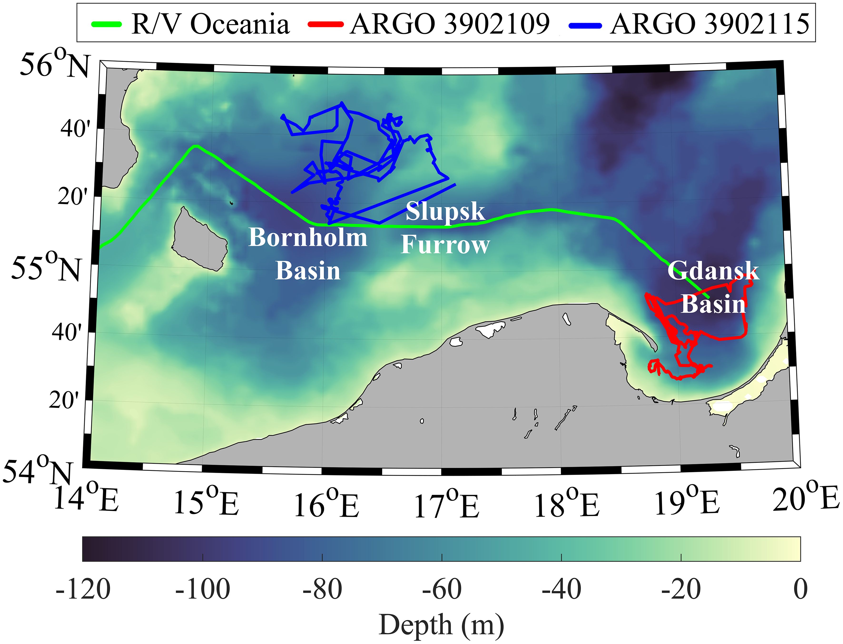
Figure 1 Measurements performed by the Argo floats no. 3902109 (red) and no. 3902115 (blue) and the R/V Oceania (green). The floats were deployed at different locations in the Southern Baltic. Meanwhile, the research vessel Oceania has been carrying out scientific expeditions since 1998.

During the initial 79 cruises, the IOPAN collected Conductivity, Temperature, and Depth (CTD) data every 0.2 nm to obtain high-resolution transects. However, due to instrument loss in May 2020, the CTD data were acquired along the same transect at intervals of 5 nm during the remaining cruises. Unfortunately, the in-situ data collected from the R/V Oceania include only few measurements from the summer months as the vessel is typically on the Arctic expedition during this time.

The IOPAN used a towed CTD frame equipped with a 24Hz SeaBird Electronics sensor to measure conductivity, temperature, and pressure (depth) with high accuracy and precision. Despite collecting transects every 5 nm, the vertical resolution of these measurements was approximately 3 cm, ensuring high-resolution data collection.

After the CTD data was collected, standard techniques were used to remove any spikes or noise. The data were then smoothed by averaging over a 0.5-meter interval to obtain profiles of temperature, salinity, and density. The density was calculated using the UNESCO formula (1981) based on the temperature and salinity profiles Unesco, 1981.

2.2 Argo floats

This study utilized data collected by two Argo floats deployed by IOPAN as part of the Argo-Poland project in the Baltic Proper between 2020 and 2023 (http://www.iopan.gda.pl/hydrodynamics/po/Argo/argo_balticfloats.html/) (Walczowski et al., 2020). Argo floats are autonomous profiling ocean monitoring devices that are equipped with sensors to measure temperature, salinity, and biogeochemical properties. The Argo float operational cycle involves submersion to a designated drifting depth, drift, submersion to the maximum measurement depth and surfacing. During this time, data from the sensors are recorded and transmitted via satellite upon surfacing. In the Southern Baltic, a series of floats have been deployed. Those areas are characterized by strong gradients in temperature, salinity, and other environmental parameters, making it an ideal location for studying oceanographic processes. Two of these floats were deployed in specific areas, with one float in the Bornholm Basin and the other in the Gdansk Deep.

Float no. 3902109 was deployed in the Gdansk Basin on June 6th, 2020, and remained active until August 1st, 2021. During its active period, it completed a total of 500 profiles, providing valuable data on the ocean conditions in the area. Meanwhile, float no. 3902115 was deployed in the Bornholm Basin on June 15th, 2021, and remains active to this day. As of February 28th, 2023, it has completed 310 profiles, adding to the dataset on sea conditions in the region.

2.3 Model data

ERA5 - global atmospheric reanalysis produced by the European Centre for Medium-Range Weather Forecasts (ECMWF). In this study, data from ERA5 (Hersbach et al., 2023) was obtained for the period from January 1987 to June 2023. Data were collected for each day at 00:00 hours and every two hours for the entire Baltic Sea region. These data were used to analyze the Annual variations of Vertical Integral of Total Energy (VITE), Top Net Short-Wave Radiation, and Sea Surface Temperature (SST) in the Southern Baltic Sea and to present the Energy Budget across the entire Southern Baltic Sea region. The ERA5 reanalysis data features a horizontal resolution of 31 km, providing more detailed and accurate information compared to the previous ERA-Interim reanalysis.

NEMOv4.0 - Baltic Sea Physics Analysis and Forecast using E.U. Copernicus Marine Service Information Numerical model providing forecasts for the physical conditions in the Baltic Sea (DOI: ttps://doi.org/10.48670/moi-00010). The product is produced by a Baltic Sea set up of the NEMOv4.0 ocean model. In this study we used the average daily mean forecasts of potential temperature for period 2021-2022. The product provided data with a resolution of 1 nautical mile horizontally and up to 56 levels of vertical depth. These data were used to calculate average differences between maximum temperature occurrence at the surface and at depths of interest. Data for Ocean mixed layer thickness (UML) analyses were obtained from the same model.

3 Methods

3.1 Data processing

In this study, the data post-processing involved multiple steps applied to the in-situ data gathered from the R/V Oceania and measurements from Argo floats prior to the later analysis. One of the first steps involved quality control, which is a method used to identify and eliminate data errors or outliers. By doing so, we can ensure that the data we analyze is of the highest quality. In the context of this study, outliers were defined as extreme values of salinity and temperature. For practical salinity units, extreme values were below 5 and above 22 in the Bornholm Basin, values below 5 and above 20 in the Slupsk Furrow, and values below 5 and above 18 in the Gdansk Deep. Similarly, for temperature, extreme values were identified as 0°C and 21°C for all regions.

The next step involved cubic spline data interpolation (De Boor and De Boor, 1978) to obtain a vertically homogeneous distribution and finally, the data were gridded into a 2nm grid to facilitate further analysis.

3.2 Energy balance estimation

The energy balance of the Baltic Sea was determined utilizing data derived from the ERA5 climate reanalysis dataset. Key components such as latent heat, sensible heat, longwave radiation, and shortwave radiation were considered in the energy balance calculation (Figure 2).

Figure 2

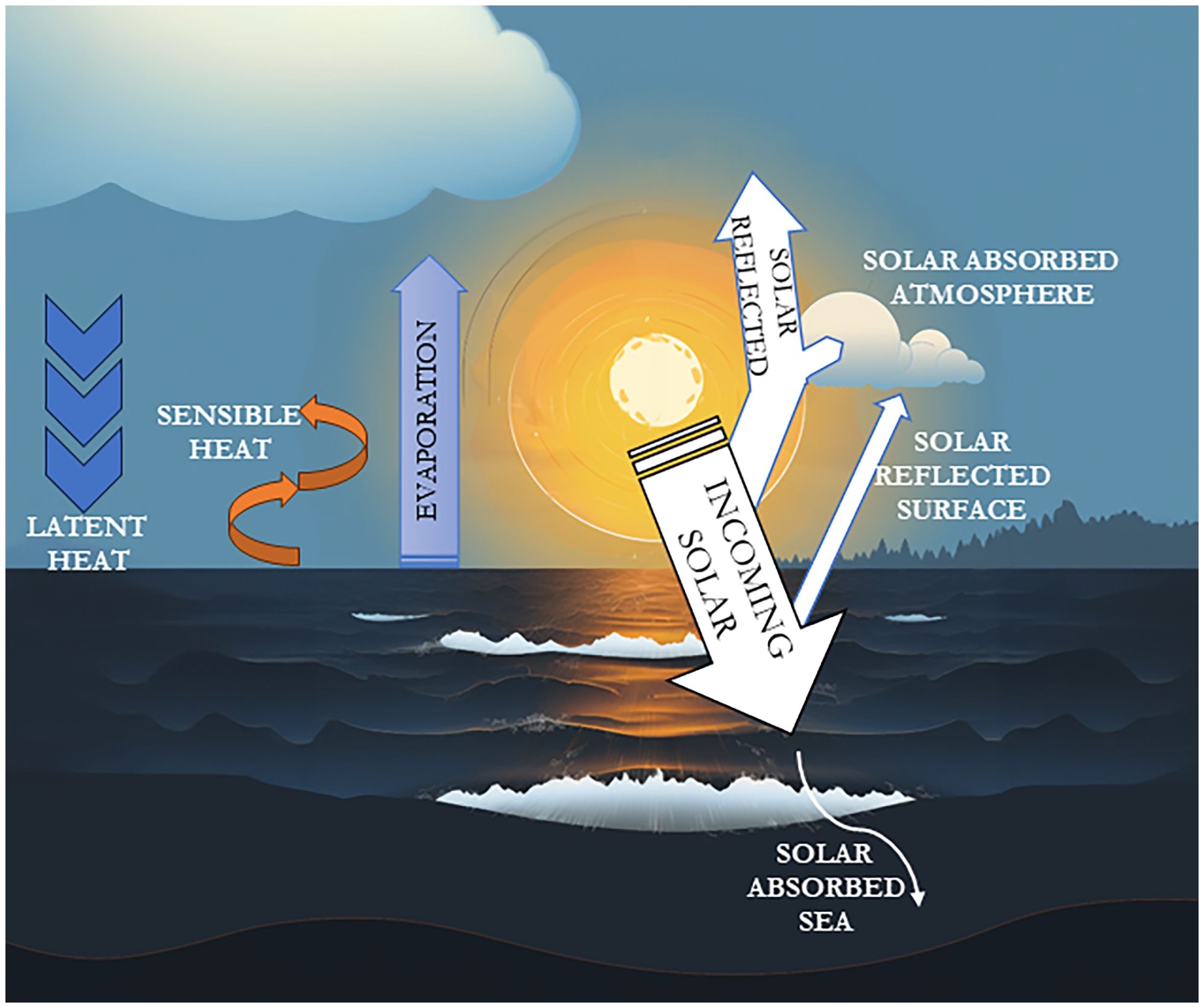
Figure 2 Energy budget over the sea, based on Wild et al. (2015).

The equation used for determining the net energy at the Earth’s surface is as follows:

$$\begin{array}{c}Net Energy = Shortwave Radiation flux + Longwave Radiation flux \\ + Latent Heat Flux + Sensible Heat Flux.\end{array}$$

Where:

Shortwave Radiation flux - The quantity of solar radiation, also referred to as shortwave radiation, that reaches a horizontal plane on the Earth’s surface includes both direct and diffuse components. This amount is reduced by the radiation reflected off the Earth’s surface, a process controlled by the Earth’s albedo. Solar radiation is partially reflected into space by clouds and atmospheric particles (aerosols), with a portion being absorbed.

Longwave Radiation flux - Thermal radiation, often termed longwave or terrestrial radiation, is emitted by the atmosphere, clouds, and the Earth’s surface. This parameter represents the net balance between downward and upward thermal radiation at the Earth’s surface, essentially the amount of radiation traversing a horizontal plane. The atmosphere and clouds continuously emit thermal radiation in various directions, with a portion of this radiation directed downwards toward the Earth’s surface as downward thermal radiation.

Latent Heat Flux - The movement of latent heat, which arises from phase changes of water like evaporation or condensation, occurs between the Earth’s surface and the atmosphere due to turbulent air motion. When water evaporates from the Earth’s surface, it transfers energy to the atmosphere.

Sensible Heat Flux - The process of sensible heat transfer, which occurs between the Earth’s surface and the atmosphere via turbulent air motion and excludes heat transfer from condensation or evaporation, is influenced by several factors. The intensity of this heat flux is determined by the temperature differential between the surface and the atmosphere above it, the speed of the wind, and the roughness of the surface.

VITE is a comprehensive metric that quantifies the cumulative energy within a vertical column of the atmosphere, extending from the Earth’s surface up to the top of the atmosphere. This integral considers all forms of energy present in the column, including internal energy, which is the energy associated with the temperature of the air; potential energy, which relates to the altitude of the air mass; kinetic energy, which accounts for the motion of air; and latent energy, which is associated with water vapor and the processes of condensation and evaporation. By synthesizing these varied energy forms, VITE allows us to determine whether seemingly minor, recurring processes play a role in shaping the broader patterns of heat transfer and energy flow within the ecosystem. The formula for calculating VITE is detailed in the work by Berrisford et al. (2011).

3.3 Seasonal changes in the temperature of the water column

Data derived from the R/V Oceania cruises spanning from 1998 to 2023, and Argo float observations collected between 2020 and 2023, were utilized for this analysis. To ensure a comprehensive examination, the study areas were delineated based on a 70 m isobath and specific longitudinal ranges for each basin:

● For the Bornholm Basin, the geographical longitude range was set between 14.7 and 16.3 degrees.

● The Slupsk Furrow was defined within the longitude range of 16.5 to 17.7 degrees.

● The Gdansk Basin’s analysis was confined to the longitude range of 18.6 to 19.4 degrees.

Data from these regions were vertically averaged at one-meter intervals and presented along the time axis. Upon aggregating these data, a curve was fitted to R/V Oceania data at each depth as a function of time, employing the Nonlinear Least Squares Method (Dennis et al., 1977) for statistical optimization and curve fitting. Due to their uneven distribution across the basins, Argo float data were utilized solely for verifying the accuracy of the curve fitting, and not for the curve fitting. This process was conducted separately for each of the three areas, utilizing the MATLAB function ‘fourier3’ for Fourier series approximation of complex temperature patterns. Figure 3 illustrates the curve fitting applied to R/V Oceania data from the surface layer of the water in the Bornholm Basin, the Slupsk Furrow, and the Gdansk Deep. This method allowed for the creation of what we have termed the ‘seasonal function of temperature,’ which represents a synthesized view of temperature changes over time at each depth level, with a 1m vertical resolution. The curve fitting on Figure 4 was applied only to data points where the correlation with the measured data exceeded 0.7, ensuring that the fitted function accurately reflects the temperature values observed in the study areas. In the next step, this method was conducted without the correlation limit for the Figure 5, showcasing the entire water column. Subsequently, the method with the 0.7 correlation limit was also applied to determine correlations, as illustrated in Figure 6.

Figure 3

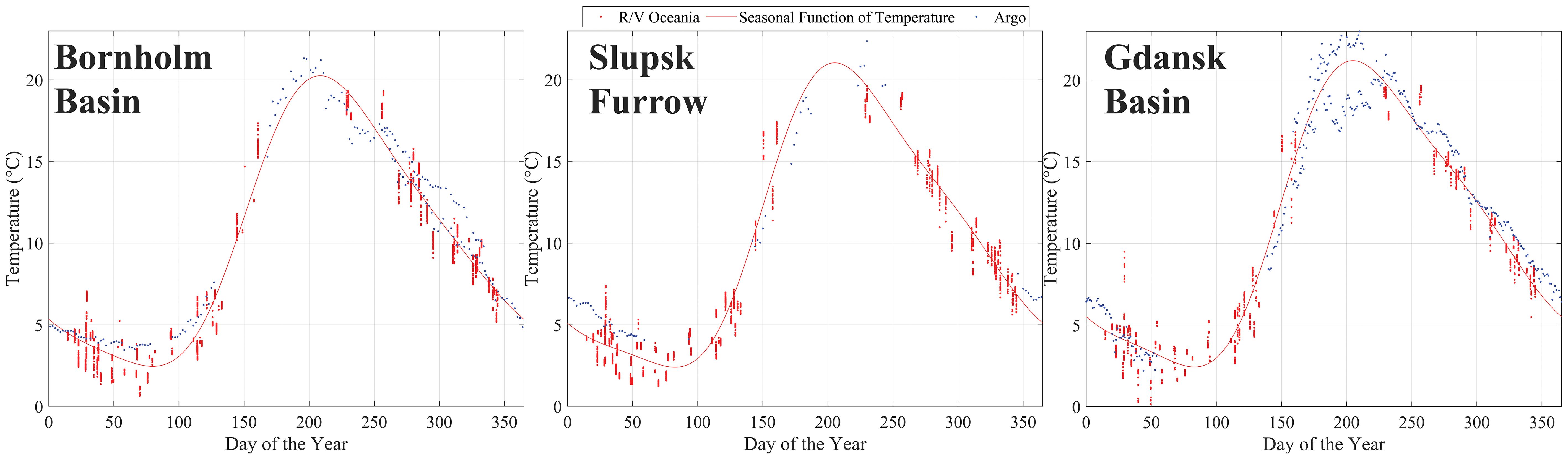
Figure 3 Seasonal function of temperature (red line) applied to observational data (blue dots) from argo floats and rv oceania across the surface water layer in the bornholm basin (left), the slupsk furrow (center), and the Gdansk.

Figure 4

Figure 4 Seasonal changes of water temperature for different depths (color scale) in the Bornholm Basin (upper plot), Slupsk Furrow (middle) and Gdansk Basin (bottom plot). Data based on R/V Oceania surveys and Argo float data.

Figure 5

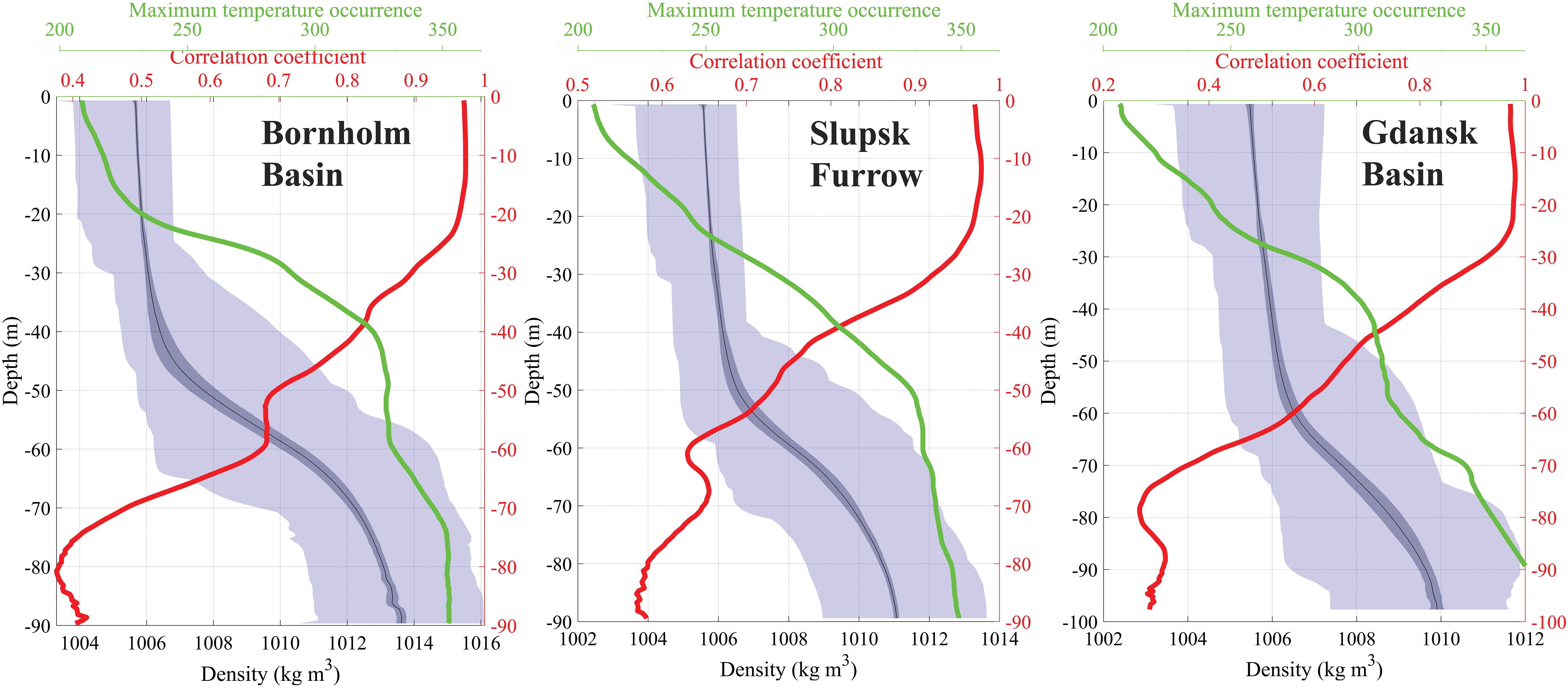
Figure 5 Density profile (blue line) and Pearson correlation coefficient (red line) and Maximum temperature occurrence (green line) in days. Analysis of seasonal temperature functions against average values (1998–2023) for the Bornholm Basin (Left), the Slupsk Furrow (Middle), and the Gdansk Basin (Right). Solid colors indicate standard deviation; transparent areas show the range of observed minimum and maximum Values.

Figure 6

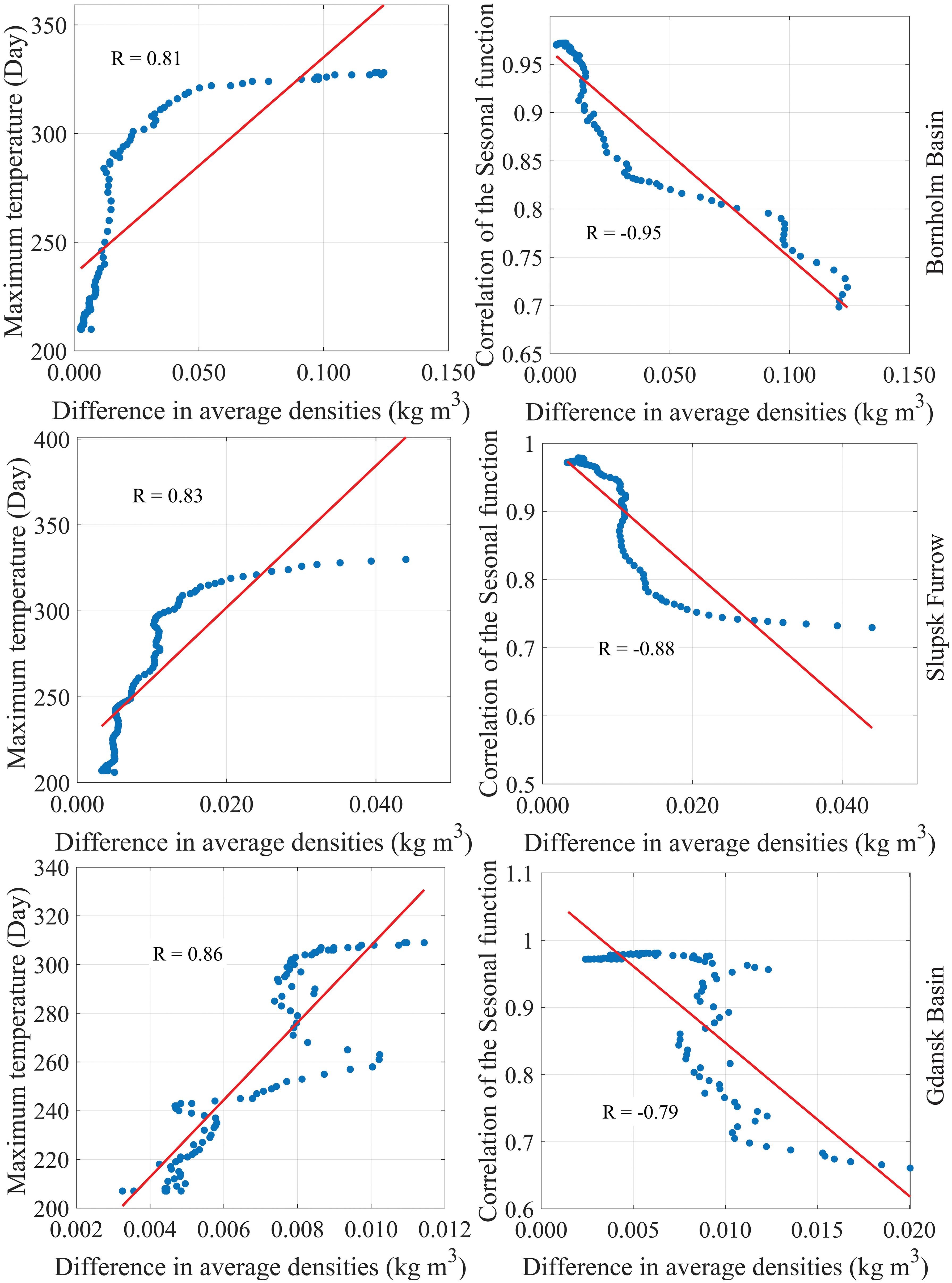
Figure 6 Pearson correlation coefficient between maximum temperature occurrence and difference in average densities (Left) vs. Pearson correlation coefficient between Pearson correlation coefficient and difference in average densities (Right) for the layer from the surface to a depth of 50 m in the Bornholm Basin, the Slupsk Furrow, and the Gdansk Basin.

4 Results

4.1 The structure of the water column in the southern Baltic Sea

The Baltic Sea is characterized by high temporal variability in temperature in the upper layer (Figure 7). This layer can extend to a depth corresponding to the halocline. Specifically, the maximum thickness of the upper layer is approximately 45-50 meters in the Bornholm Basin, 50-55 meters in the Slupsk Furrow, and increases to 60-65 meters in the Gdansk Deep. In the upper layer, variability is induced by the annual heating-cooling cycle and formation of the thermocline. The smallest temperature variation takes place in the bottom layer, with average temperatures in the Bornholm Basin at approximately 6.9 ± 2°C, in the Gdansk Deep around 6.9 ± 1°C, and in the Slupsk Furrow near 7.5 ± 1.6°C. A similar pattern was previously reported by Schmidt et al. (2021).

Figure 7

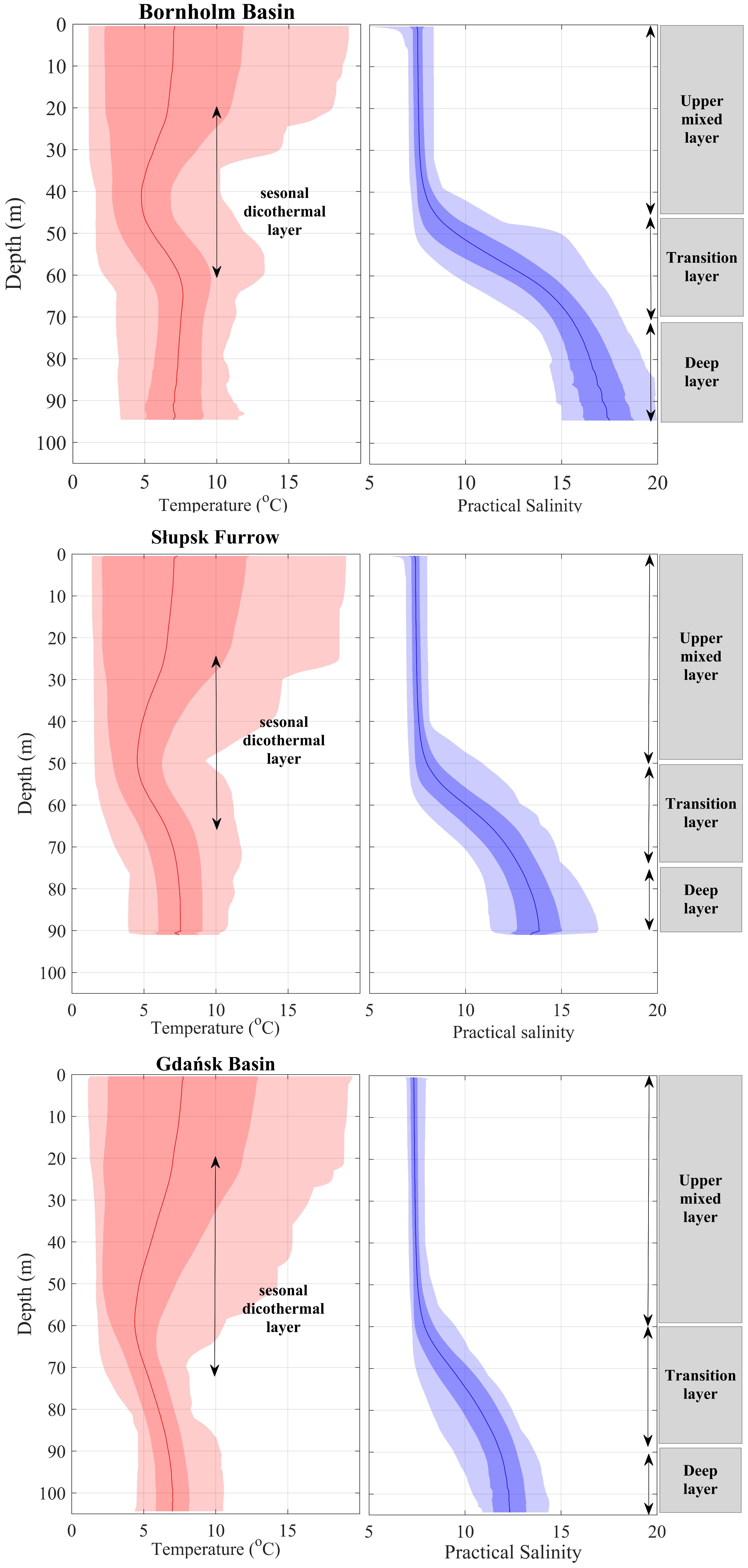
Figure 7 The structure of the water column in the Bornholm Basin (upper plot), Slupsk Furrow (middle) and Gdansk Deep (lower plot). Data based on R/V Oceania surveys and Argo float data. In these plots, solid lines indicate average temperature (red) and salinity (blue) values. Areas filled with solid colors represent the standard deviation, whereas transparent areas depict the range of minimum and maximum values observed.

The Baltic Sea exhibits minimal seasonal surface salinity variations (average practical salinity 7.3 ± 0.2) across all regions, with changes intensifying with depth and reaching their peak at the seabed. Notably, these variations are more pronounced in the Bornholm Basin compared to the deeper Gdansk Basin (Figure 7).

A study of the Bornholm Basin, Slupsk Furrow, and Gdansk Deep has shown that while the variability in these regions is similar, the extent to which thermocline penetrates the water column is limited or slowed down by the dicothermal layer. The upper boundary of this layer starts at a surface, but it experiences seasonal variations due to the continued delivery of solar energy, which leads to the deepening of the thermocline, thereby reducing the thickness of the dicothermal layer. In contrast, the lower boundary of the dicothermal layer aligns with the halocline level, undergoing changes primarily during events of dense water advection. Consequently, the maximum thickness of this layer in the Bornholm Basin is about 40 meters, whereas in the Gdansk Deep, it extends to 60 - 70 m. Therefore, the greater thickness of the dicothermal layer cause the dictothermal leyer to survive until the next cold season in the Gdansk Basin. The average minimum temperature of this layer is approximately 4.7°C ± 2°C in the Bornholm Basin and 4.3°C ± 1°C in the Gdansk Deep.

4.2 Radiation and energy fluxes in the surface water of the southern Baltic Sea

Figure 8 presents the energy flow through the surface layer of the Southern Baltic Sea, corresponding to the area outlined in Figure 1. The energy balance of this region is significantly influenced by the flux of short-wave (solar) and long-wave (terrestrial) radiation. Diurnally, energy absorption by the Baltic Sea is variable, with energy release indicated by negative values during nighttime hours. With the break of dawn and into the morning, the region begins to absorb energy, typically peaking at 238.55 W m^-2 around 10 AM, suggesting the time of maximum solar energy absorption. This absorption continues, with the highest values observed from 8 AM to 4 PM. As evening approaches, the energy flux diminishes, leading to energy release after sunset. Seasonally, the Baltic Sea’s energy budget follows a cyclical pattern influenced by variations in daylight and solar elevation. Negative energy values during winter, dropping to -120 W m^-2 in December, reflect the region’s energy emission due to limited solar radiation. This emission is counterbalanced by increased absorption beginning in spring, reaching a peak in June, and then decreasing after the summer solstice as part of the annual cycle. The overall annual energy budget for the Southern Baltic is characterized by a net positive mean value of 5.48 W m^-2, indicating that, on average, the region absorbs more energy than it releases over the course of a year, effectively acting as an energy sink.

Figure 8

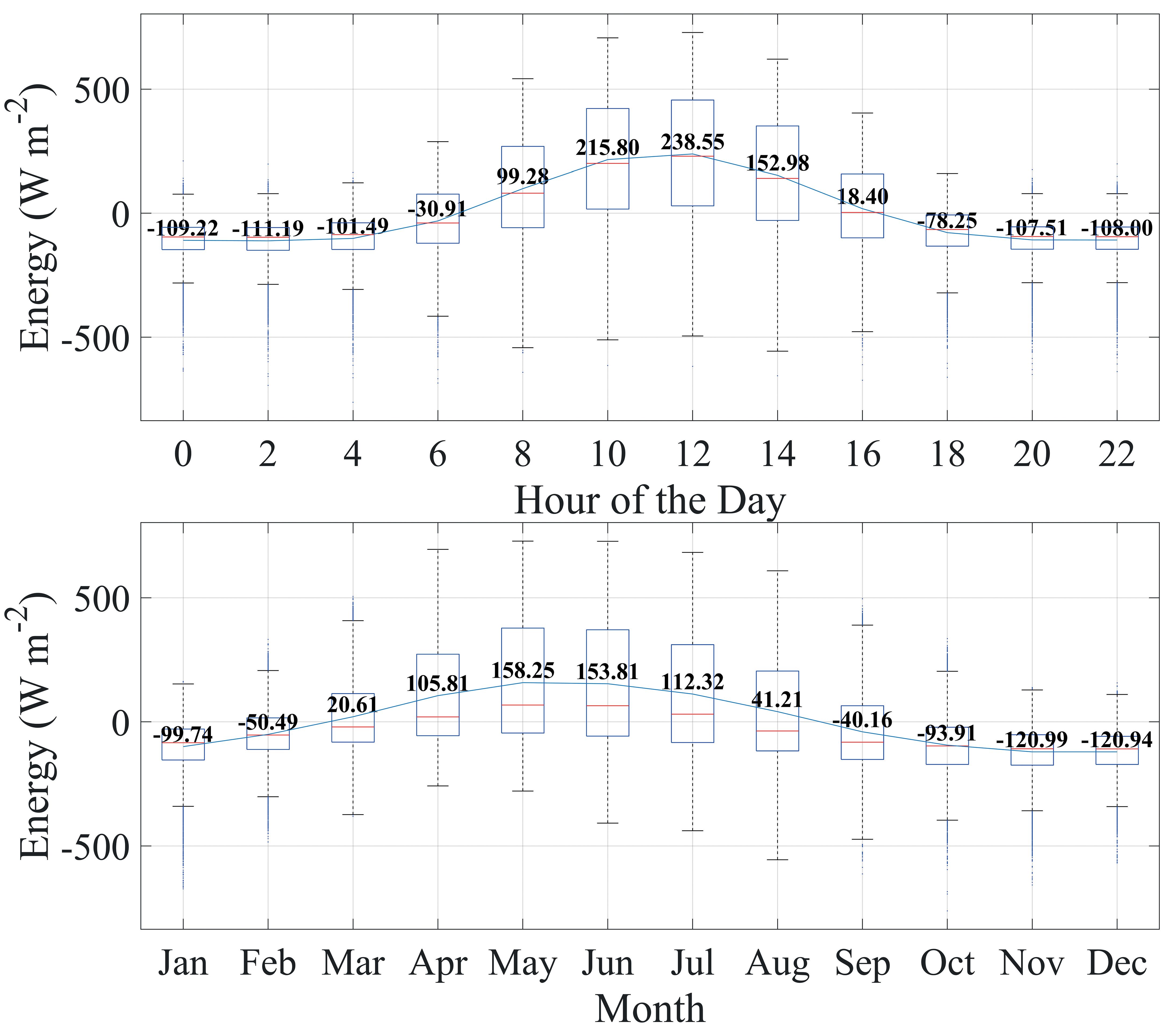
Figure 8 Energy Budget of the Southern Baltic Sea’s Surface based on the analysis of energy components from 1987 to 2023. The upper diagram depicts daily changes, and the lower diagram shows seasonal variations. The blue solid line represents the mean values.

Figure 9 displays the average distribution of VITE in the Southern Baltic Sea between 1987 and 2023. While the average value sits at 2.61 x 10⁹ J m^-2, the data reveals significant spatial variability across the region. This variation is primarily driven by latitude, as areas receiving more solar radiation tend to exhibit higher VITE values. Gotland Deep, for instance, boasts a VITE of 2.614 x 10⁹ J m^-2, compared to 2.625 x 10⁹ J m^-2 in the Bornholm Basin, reflecting the differing levels of solar radiation they receive due to their respective latitudes. However, the picture is not solely painted by latitude. Local factors also play a crucial role in shaping the VITE distribution. Upwelling zones, like the one near Debki, exhibit VITE values of 2.619 x 10⁹ J m^-2, which is higher than in areas at similar latitudes without such events, by roughly 5.5871 x 10⁶ J m^-2. Additionally, freshwater inputs from major rivers like the Vistula and Oder significantly impact the distribution. These influxes can alter the thermal structure of the sea locally, thereby influencing VITE, particularly near river mouths.

Figure 9

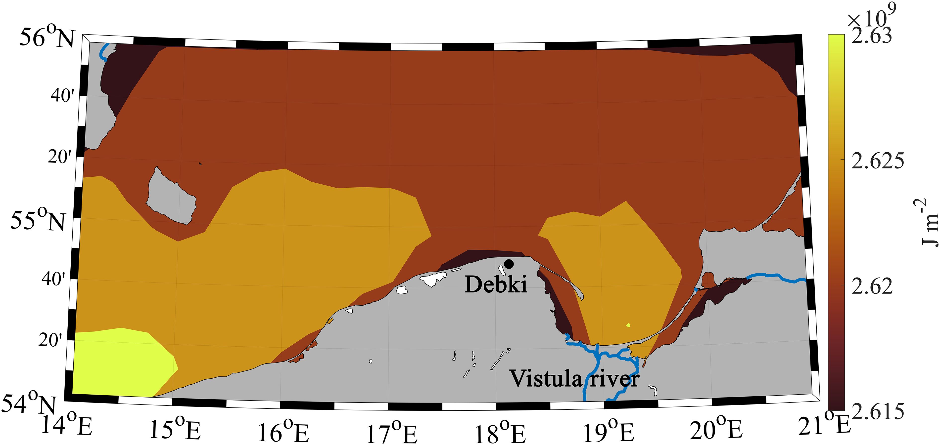
Figure 9 Average distribution of the VITE in the Southern Baltic Sea, based on ERA-5 data from 1987 to 2023.

Every year, the Southern Baltic region receives its peak solar energy input (Figure 10), on average, around the 169th day of the year (June 18th). This energy, quantified as 3.51 x 10⁶ Joules per square meter (J m^-2), is absorbed by the atmosphere and the ocean surface, instigating the gradual warming process. However, the maximum absorption and internal distribution of this energy, encapsulated by the VITE, does not occur instantaneously. Therefore, VITE peaks slightly later, on average, around the 210th day of the year (July 29th). This delay is indicative of the time it takes for the atmosphere to absorb and redistribute the heat energy derived from the sun. Further down the timeline, we observe the peak SST. The temperature of the sea surface does not crest until the 216th day of the year, roughly around August 4th. This additional delay, compared to the VITE, can be attributed to the water high heat capacity - the ability of water to absorb a considerable amount of heat without experiencing a significant change in its own temperature. Therefore, the sea takes in a lot of energy over time, gradually warming until it reaches its peak temperature.

Figure 10

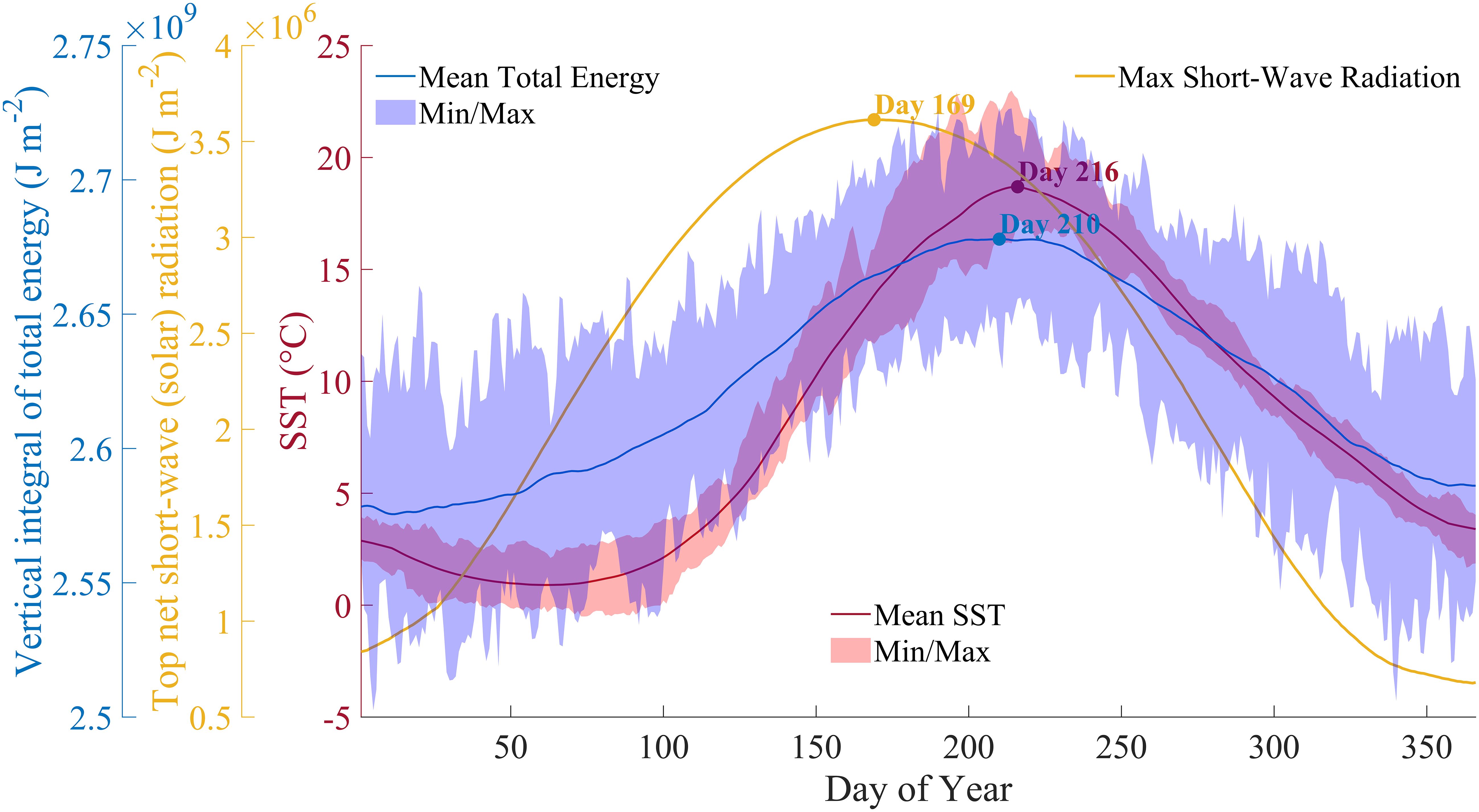
Figure 10 Annual variations of VITE, Top Net Short-Wave Radiation, and SST in the Southern Baltic Sea, based on data ERA-5 from 1987 to 2023.

4.3 Heat transfer in the Southern Baltic Sea

Given the proximity in distances, the temperature variations across the examined regions (the Bornholm Basin, the Slupsk Furrow, and the Gdansk Deep) are fairly consistent at the surface level. Notably, the highest point of the temperature’s seasonal pattern at this level typically falls on the 210th day of the year, which is July 29. This peak time experiences a phase delay as the depth increases, as shown in Figure 4. On average, for every additional 10 meters of depth, the examined areas exhibit a phase delay of about 24 days in the seasonal temperature pattern.

However, these changes are not uniform; the signal’s fastest propagation is up to a depth of 25 meters, beyond which it slows down. The correlation between the measured data and their seasonal pattern remains high, around 0.9, up to a depth of approximately 25 meters, as indicated in Figure 5. Nonetheless, at depths of 20 to 22 meters across all sub-basins, there’s a marked decline in this correlation. This drop is associated with the upper boundary of the thermocline, as evident in the density profile.

As depth increases, so does the phase shift of the pattern, reflecting the time needed for the surface temperature signal to reach deeper levels. The speed of this signal transmission varies among the basins, fastest in the Gdansk Deep and slowest in the Bornholm Basin. At around 45 meters deep, the maximum phase shift difference between the Bornholm Basin and the Gdansk Deep is 19 days, accompanied by a variation in amplitude that is lesser in the Bornholm Basin up to this depth. Beyond 50 meters, the correlation progressively weakens, dropping to 0.7 at around 45 meters in the Gdansk Deep. Past the halocline, the correlation sharply decreases, underscoring a diminished link between deep water temperature fluctuations and atmospheric conditions. The Gdansk Basin exhibits a quicker reduction in correlation compared to the Bornholm Basin and the Slupsk Furrow, likely due to a prolonged Cold Intermediate Layer (CIL) presence.

A second significant correlation coefficient drop is observed at depths of 38 meters in the Bornholm Basin, 42 meters in the Slupsk Furrow, and 45 meters in the Gdansk Basin, as shown in Figure 5. These shifts correlate with the mixed layer’s base. The relationship between signal propagation speed, seasonal function correlation (indicative of the curve fitting quality to the measured values), and difference of density—which shapes the vertical water structure of the Baltic Sea—is depicted in Figure 6. Here, the correlation between these parameters ranges from approximately 0.79 to 0.95, indicating a moderate to strong dependency.

It’s crucial to acknowledge that the functions for the upper mixed layer, presented in Figure 4, are truncated at varying depths in each basin based on a set 0.7 correlation coefficient threshold. Specifically, seasonal functions are discontinued at depths of 45 meters in the Gdansk Basin, 53 meters in the Slupsk Furrow, and 49 meters in the Bornholm Basin. Despite the sharp drop in correlation below the halocline, Figures 6, 11 visualize the entire water column, even beyond depths where the correlation significantly decreases beyond 0.7.

Figure 11

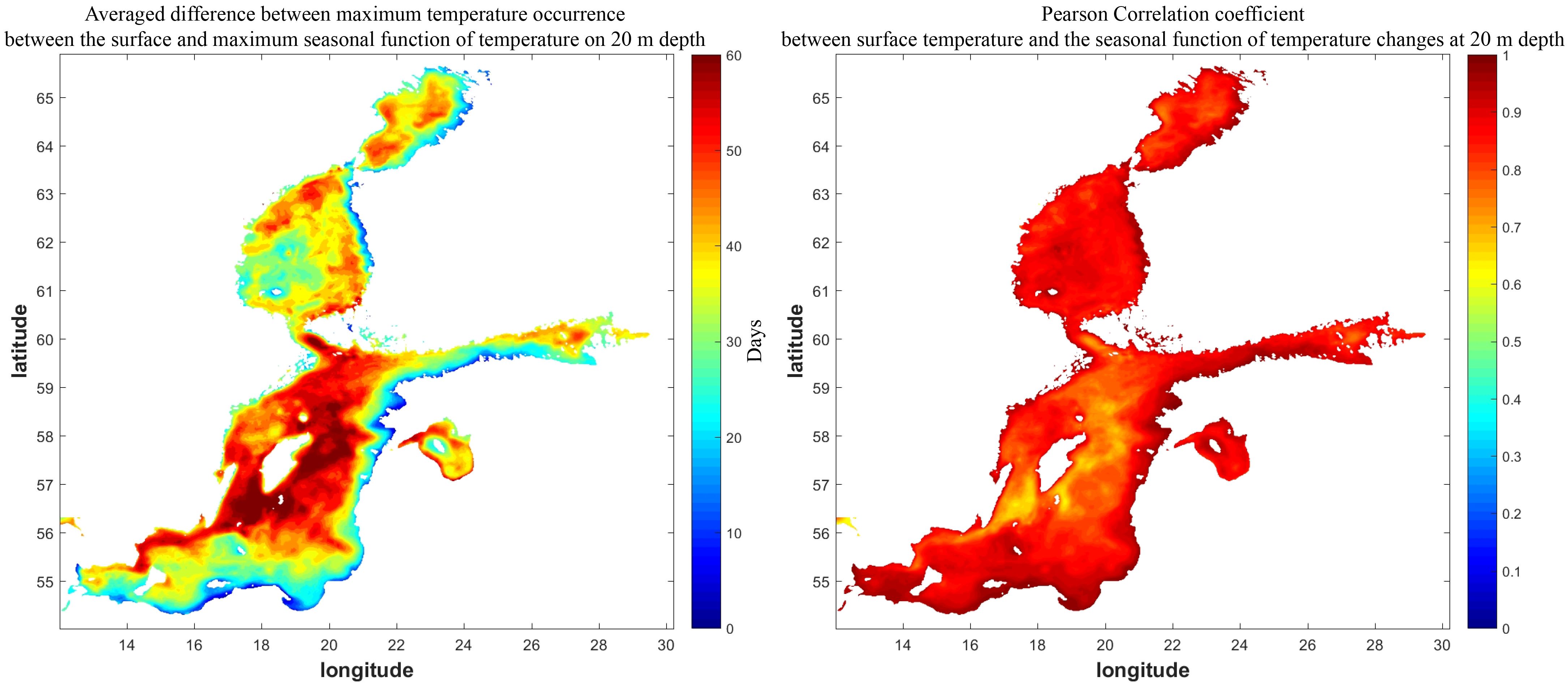
Figure 11 Averaged (2021-2022) difference between maximum temperature occurrence between the surface and maximum seasonal function of temperature on 20 m depth (left) and the Pearson correlation coefficient between surface temperature and the seasonal function of temperature changes at 20 m depth (right).

4.4 Analysis of heat propagation speed across the Baltic Sea

In the course of this study, we conducted a detailed reanalysis to quantify the vertical heat transport within the Baltic Sea. By leveraging the seasonal temperature function (Section 3.3), applied to areas such as the Bornholm Basin, Slupsk Furrow, and Gdansk Deep, we aimed to expand upon our preliminary observations and explore broader patterns of thermal variability across the entire Baltic. Therefore, the averaged (2021-2022) difference between the peak of seasonal temperature occurrence at the surface and the maximum seasonal function of temperature at a depth of 20 meters, along with the Pearson correlation coefficient between surface temperature and the seasonal function of temperature changes at 20 meters depth, has been presented for the whole Baltic Sea (Figure 11).

Specifically, the data reveals a noteworthy pattern concerning temperature shifts in the Baltic Sea. On average, the maximum temperature between the surface and a depth of 20 m experiences a delay of about 35 days. This temporal delay in temperature is particularly pronounced when comparing different regions of the Baltic.

In the Southern Baltic, a unique trend emerges. Here, the temperature reaches its maximum at 20 m depth notably faster than in its central and northern counterparts. When quantified, this difference amounts to about 40 days. It has been noted that the shorter the interval between the surface temperature peak and that at 20 m depth, the greater the correlation becomes between the seasonal function of temperature changes at this depth.

Additionally, it is important to highlight that there is a decrease in the Pearson correlation coefficient between surface temperature and the seasonal temperature change function at a depth of 20 meters. Specifically, in the Central Baltic, the correlation decreases significantly when there is a large discrepancy (50 or more days) between the occurrence of maximum surface temperature and the peak of the seasonal temperature function at 20 meters depth. Furthermore, during the analysis period, which covered the full years of 2021-2022 (with complete model data available only for these years), significant differences were observed between the eastern and western shores of the Baltic Sea.

Figure 12 represents averaged (2021-2022) maximum depth of Upper Mixed Layer in the Baltic Sea. A greater thickness of the Upper Mixed Layer (UML) is expected in deeper areas. In deeper areas of the Baltic Sea, the water’s response to temperature changes is slower due to its greater volume and depth. This leads to a delayed transmission of heat to these deeper layers, affecting the temperature profile and its correlation with surface measurements.

Figure 12

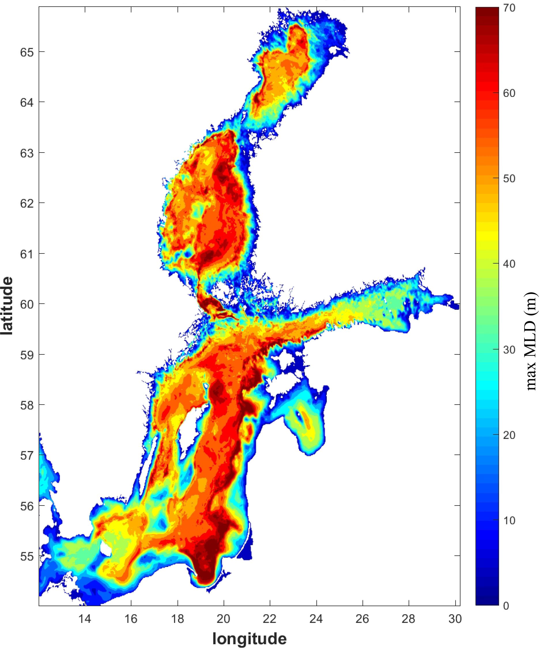
Figure 12 Averaged (2021-2022) maximum depth of Upper Mixed Layer in the Baltic Sea (NEMOv4.0).

Furthermore, the Upper Mixed Layer (UML) is closely linked to bathymetry and bottom advection. These two parameters significantly influence the halocline level and thus play a crucial role in determining the temperature distribution and dynamics of the UML. The correlation between the maximum UML (Upper Mixed Layer) and bathymetry in the Baltic Proper is illustrated in Figure 13, which shows that it is very high at level 0.85, indicating a close relationship between the maximum depth of the UML and bathymetry. While the minimum depth of the UML, defined by the depth at which the thermocline forms, its maximum depth is primarily conditioned by the depth of the halocline. In the central area of the Bornholm Basin, the maximum depth of the UML is greater due to a higher halocline (about 45-50 m). Conversely, in the Gdansk Deep, the maximum depth of the UML reaches up to 70 meters.

Figure 13

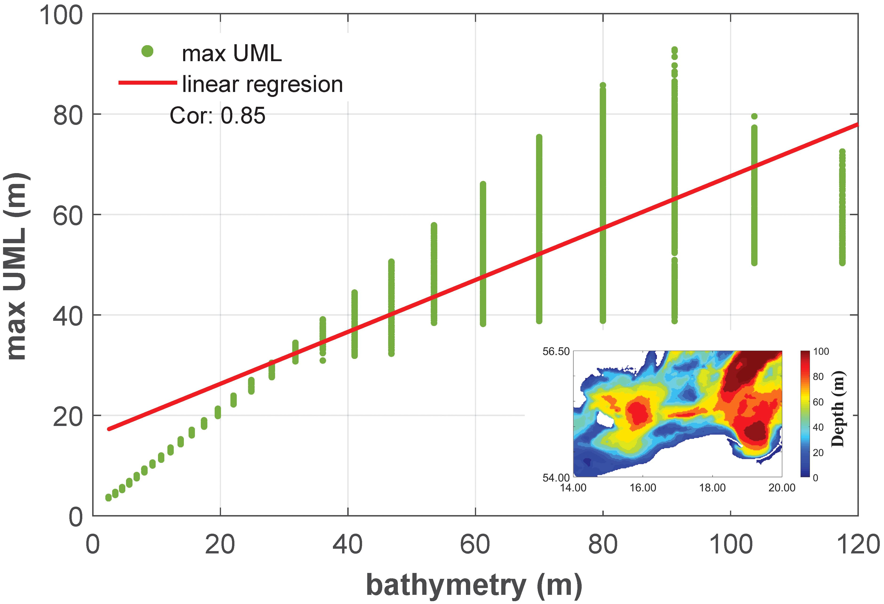
Figure 13 Correlation between the maximum UML (Upper Mixed Layer) depth and bathymetry in the Baltic Proper.

In shallower regions, devoid of a distinct halocline, the maximum extent of the Upper Mixed Layer (UML) is not constrained in the same way and can reach all the way to the seabed. In these areas, the absence of a pronounced halocline allows for a more extensive vertical mixing, which results in the UML potentially encompassing the entire water column depth.

5 Discussion

The case of the Southern Baltic Sea offers an insightful look into the structure of the water column and energy fluxes. These findings discussed in sections 4.1 and 4.2, emphasize the notable variability in temperature within the Baltic Sea, with a special focus on the upper layer. These findings align with established knowledge of the Baltic Sea’s temperature variability, an attribute significantly affected by annual heating-cooling cycles and thermocline formation (Stockmayer and Lehmann, 2023). The study found that the Top Net Short-Wave Radiation, essentially the sun-derived short-wave radiation remaining after accounting for the energy reflected to space, peaks annually around June 18th, the 169th day of the year (Figure 10). This energy, approximately 3.51 x 10⁶ J m^-2, is absorbed by the atmosphere and ocean surface, instigating a gradual warming process. However, VITE, which encapsulates the peak absorption and distribution of this energy, does not immediately follow this trend. This lag, which sees VITE peaking around July 29th, the 210th day of the year, illustrates the time necessary for atmospheric absorption and redistribution of solar heat energy. This delay also extends to the peak SST, observed around August 4th, the 216th day of the year. This additional delay can be attributed to water’s high heat capacity, signifying its ability to absorb significant amounts of heat without considerable temperature change.

The energy budget analysis of the study shows an annual average of 5.48 W m^-2 for the region, highlighting the Southern Baltic’s function as a net energy sink (Figure 8). This contributes to the storage of heat in the ocean and may influence wider climatic patterns. Typically, the Southern Baltic absorbs energy daily from 8 AM to 4 PM. The highest rate of energy absorption in the Baltic occurs in May/June, with an average of 158 W m^-2. In contrast, November sees the energy emission by the sea, with the region experiencing a net energy loss of -120 W m^-2. From August to March, the Southern Baltic shifts to emitting more energy into the atmosphere than it absorbs. This regional energy exchange pattern complements global observations, where unadjusted estimated surface fluxes align with observed heat absorption up to 1 W m-², indicating consistency in energy dynamics at both global and regional scales (Mayer et al., 2022).

Moreover, this study underscores the necessity to comprehend the spatial and temporal variability in energy distribution. With latitude playing a significant role, the VITE exhibits substantial spatial variability across the Southern Baltic Sea (Figure 9). Interestingly, the spatial distribution of reduced VITE areas, as depicted in this study, aligns remarkably well with the regions of upwelling and downwelling identified in the work by Kowalewski and Ostrowski (2005), which focused on coastal up- and downwelling in the southern Baltic. This relationship indicates a strong link between those events and the noted reduction in VITE, implying a dynamic feedback mechanism of the sea to the atmosphere. It highlights a multifaceted interaction between environmental factors and the energy dynamics of the sea. However, we must acknowledge the limitations posed by the coarse spatial resolution of the ERA5 data. It is important to highlight that our conclusions regarding the spatial distribution of VITE may require further, deeper analysis as models with higher spatial resolution become available and are refined. The coarse spatial resolution of ERA5 data renders the connection between VITE spatial variability and specific phenomena such as upwelling zones and river plume areas somewhat imprecise.

In the water column structure, the dicothermal layer is critical, regulating the thermocline’s penetration (Dargahi et al., 2017). The differences in the dicothermal layer’s depth and extent across various regions underscore the marine ecosystem’s complexity in the Baltic Sea (Liblik and Lips, 2019). Hence, understanding factors influencing heat transfer within the Southern Baltic Sea, such as the halocline level and advection processes, is essential. These factors impact the thickness of the dicothermal layer and, consequently, the seasonal signal’s propagation deep into the water column. Regarding the surface layer, spatial temperature variations align with latitude changes. Due to the small spatial differences between the study areas — the Bornholm Basin, Slupsk Furrow, and Gdansk Deep — similar trends in temperature changes are observed in the surface layer up to a depth of about 20 meters (Figure 5).

In the Southern Baltic Sea, the peak surface temperature emerges two months after the thermocline forms (Janecki, 2022). The highest and lowest points of the seasonal function appear around July 29 (day 210) and March 21 (day 80), respectively (Figure 5). The data within the surface aligns closely with its derived seasonal function, with a correlation of about 0.97. Generally, for every added 10 meters in depth, the temperature phase shift is delayed by around 24 days.

Past the surface layer, the function’s phase shift alters, indicating the time to convey the temperature signal deeper. This signal’s speed differs among basins—it’s quickest in the Gdansk Deep and slowest in the Bornholm Basin. At roughly 45 meters depth, the Bornholm Basin and the Gdansk Deep have a 19-day phase shift difference in the seasonal function. This phase change also comes with amplitude variation, with the amplitude being reduced in the Bornholm Basin to a depth of 45 meters.

The relationship between the day of maximum occurrence and seasonal function correlation (indicative of the curve fitting quality to the measured values), suggests that vertical heat transport is constrained by density differences (Figure 6), first becoming evident at a depth of 25 meters due to the thermocline (Figure 5). Subsequent declines in correlation occur at 38 meters in the Bornholm Basin, 42 meters in the Slupsk Furrow, and 45 meters in the Gdansk Basin, indicating a reduced connection between deeper water temperatures and surface conditions, aligning with the base of the mixed layer.

The noticeable seasonal function beneath the halocline is mainly driven by advection rather than local convection or surface events. The waters sinking into the Baltic Sea’s depths from the North Sea’s surface have a high density, leading them to carry a strong signal of seasonal changes. In the Bornholm Basin and Slupsk Furrow, seasonal variations are largely influenced by advection, significantly enhanced by frequent baroclinic and less frequent but stronger barotropic inflows. Research by Lehmann and Post (2015), and Mohrholz (2018) provides detailed insights into this process.

Furthermore, during the period for which the numerical analysis was conducted, spanning the full years of 2021-2022, the results corroborated the findings from the in situ data analysis. It was observed that the temporal gap between the occurrence of peak temperatures at the surface and at a depth of 20 meters maintains a consistent span of approximately 20 days in both the Southern and Northern Baltic (Figure 11). In the Central Baltic, however, this time difference increases. Unfortunately, this increase is accompanied by a diminishing correlation, indicating that while the delay in peak temperature is more pronounced in the Central Baltic, the relationship between surface and subsurface temperatures becomes less predictable and more variable while shifting northward.

The observed decreasing correlation in thermocline dynamics in the Baltic Sea can be attributed to the deepening of the thermocline and changes in the Upper Mixed Layer – UML (Figure 12). This deepening affects the precision of data fitting to the seasonal curves. Notably, the UML in the Baltic Sea reaches its maximum thickness toward the year’s end, especially during winter storms (Liblik et al., 2020; Bulczak et al., 2024). Furthermore, the UML attains its greatest thickness more rapidly in shallower regions, highlighting the significant influence of bathymetry on these processes (Jakobsson et al., 2019). Additionally, Larsén et al. (2006) highlighted the significance of air-sea exchange of sensible heat over the Baltic Sea, indicating that strong winds can significantly deepen the lower boundary of the UML.

6 Conclusions

In conclusion, this study emphasizes the multifaceted dynamics of thermal energy exchange within the Southern Baltic Sea and its profound implications for our understanding of marine heat transfer and climate processes. Key findings include:

1. The Southern Baltic Sea, with an average energy absorption of 5.48 W m^-2, functions as a net energy sink.

2. The Southern Baltic predominantly absorbs energy during the day from 8 AM to 4 PM, but from September to February, it emits more energy than it absorbs.

3. There is a 59-day lag between peak solar energy and the Vertical Integral of Total Energy (VITE), with an additional 6-day delay before peak Sea Surface Temperature (SST).

4. The dicothermal layer governs thermocline penetration into the water column and affects the rate of thermal energy propagation within the water, leading to a 24-day delay in temperature phase shift per 10 meters depth, extending to 35 days in Central and Northern Baltic.

Data availability statement

The raw data supporting the conclusions of this article will be made available by the authors, without undue reservation.

Author contributions

DR: Conceptualization, Investigation, Methodology, Software, Supervision, Validation, Visualization, Writing – original draft, Writing – review & editing. AP: Methodology, Software, Visualization, Writing –original draft, Writing – review & editing. AB: Methodology, Software, Visualization, Writing – original draft, Writing – review & editing. LD-G: Writing – original draft, Writing – review & editing.

Funding

The author(s) declare financial support was received for the research, authorship, and/or publication of this article. This publication was supported by the following projects: The Argo-Poland project funded by the Polish Minister of Education and Science [grant number 2022/WK/04]; CSI-POM, financed from the state budget under the program of the Polish Minister of Science entitled “Science for Society” No. NdS/546027/2022/2022; SufMix, financed by the National Science Center, Poland, the OPUS 17 program, contract no. UMO-2019/33/B/ST10/02189. This study has been conducted using E.U. Copernicus Marine Service Information; DOI: https://doi.org/10.48670/moi-00010.

Conflict of interest

The authors declare that the research was conducted in the absence of any commercial or financial relationships that could be construed as a potential conflict of interest.

Publisher’s note

All claims expressed in this article are solely those of the authors and do not necessarily represent those of their affiliated organizations, or those of the publisher, the editors and the reviewers. Any product that may be evaluated in this article, or claim that may be made by its manufacturer, is not guaranteed or endorsed by the publisher.

References

Bagaev A. V., Bukanova T. V., Chubarenko I. P. (2021). Spring cold water intrusions as the beginning of the cold intermediate layer formation in the Baltic Sea. Estuarine. Coast. Shelf. Sci. 250, 107141. doi: 10.1016/j.ecss.2020.107141

CrossRef Full Text | Google Scholar

Berrisford P., Dee D. P., Poli P., Brugge R., Fielding M., Fuentes M., et al. (2011). The ERA-Interim archive Version 2.0. ERA Report Series, (1) (ECMWF), 23. Available at: https://www.ecmwf.int/sites/default/files/elibrary/2011/8174-era-interim-archive-version-20.pdf

Google Scholar

Bulczak A. I., Nowak K., Rak D., Jakacki J., Muzyka M., Walczowski W. (2024). Seasonal Variability and Long-Term Winter Shoaling of the Upper Mixed Layer in the Southern Baltic Sea, submitted to Continental Shelf Research. doi: 10.21203/rs.3.rs-3973366/v1

CrossRef Full Text | Google Scholar

Chubarenko I., Stepanova N. (2018). Cold intermediate layer of the Baltic Sea: Hypothesis of the formation of its core. Prog. Oceanography. 167, 1–10. doi: 10.1016/j.pocean.2018.06.012

CrossRef Full Text | Google Scholar

Dargahi B., Kolluru V., Cvetkovic V. (2017). Multi-layered stratification in the Baltic sea: Insight from a modeling study with reference to environmental conditions. J. Mar. Sci. Eng. 5, 2. doi: 10.3390/jmse5010002

CrossRef Full Text | Google Scholar

De Boor C., De Boor C. (1978). “A Practical Guide to Splines,”, vol. 27. (springer-verlag, New York), 325. doi: 10.2307/2006241

CrossRef Full Text | Google Scholar

Dennis J. E., Gay D. M., Welsch R. E. (1977). An Adaptive Nonlinear Least-Squares Algorithm. Report TR 77-321 (Cornell University: Department of Computer Sciences).

Google Scholar

Döös K., Meier H. E. M., Döscher R. (2004). The Baltic haline conveyor belt or the overturning circulation and mixing in the Baltic. AMBIO.: A. J. Hum. Environ. 33, 261–266. doi: 10.1579/0044-7447-33.4.261

CrossRef Full Text | Google Scholar

Döscher R., Meier H. E. (2004). Simulated sea surface temperature and heat fluxes in different climates of the Baltic Sea. Ambio 33, 242–248. doi: 10.1639/0044-7447(2004)033[0242:SSSTAH]2.0.CO;2

PubMed Abstract | CrossRef Full Text | Google Scholar

Eilola K., Rosell E. A., Dieterich C., Fransner F., Höglund A., Meier M. (2012). Modeling nutrient transports and exchanges of nutrients between shallow regions and the open baltic sea in present and future climate. AMBIO 41, 586–599. doi: 10.1007/s13280-012-0322-1

PubMed Abstract | CrossRef Full Text | Google Scholar

Feistel R., Nausch G., Wasmund N. (2008). State and evolution of the Baltic Sea 1952-2005: A detailed 50-year survey of meteorology and climate, physics, chemistry, biology, and marine environment (Hoboken, New Jersey, USA: John Wiley & Sons). doi: 10.1002/9780470283134

CrossRef Full Text | Google Scholar

Hersbach H., Bell B., Berrisford P., Biavati G., Horányi A., Muñoz Sabater J. (2023). ERA5 hourly data on single levels from 1940 to present (Copernicus Climate Change Service (C3S) Climate Data Store (CDS). doi: 10.24381/cds.adbb2d47

CrossRef Full Text | Google Scholar

Jakobsson M., Stranne C., O’Regan M., Greenwood S. L., Gustafsson B., Humborg C., et al. (2019). Bathymetric properties of the baltic sea. Ocean. Sci. 15, 905–924. doi: 10.5194/os-15-905-2019

CrossRef Full Text | Google Scholar

Janecki M., Dybowski D., Rak D., Dzierzbicka-Głowacka L. A. (2022). A New Method for Thermocline and Halocline Depth Determination at Shallow Seas. Journal of Physical Oceanography 52(9). doi: 10.1175/JPO-D-22-0008.1

CrossRef Full Text | Google Scholar

Kowalewski M., Ostrowski M. (2005). Coastal up- and downwelling in the southern Baltic. Oceanologia 47/4, 453–475.

Google Scholar

Larsén X., Smedman A., Högström U. (2006). Air–sea exchange of sensible heat over the Baltic Sea. Q. J. R. Meteorol. Soc. 130, 519–539. doi: 10.1256/qj.03.11

CrossRef Full Text | Google Scholar

Launiainen J., Cheng B., Uotila J., Vihma T. (2001). Turbulent surface fluxes and air–ice coupling in the Baltic Air–Sea–Ice Study (BASIS). Ann. Glaciol. 33, 237–242. doi: 10.3189/172756401781818293

CrossRef Full Text | Google Scholar

Lehmann A., Post P. (2015). Variability of atmospheric circulation patterns associated with large volume changes of the Baltic Sea. Adv. Sci. Res. 12, 219–225. doi: 10.5194/asr-12-219-2015

CrossRef Full Text | Google Scholar

Leppäranta M., Myrberg K. (2009). “Topography and hydrography of the baltic Sea,” in Physical Oceanography of the Baltic Sea (Springer Berlin Heidelberg, Berlin, Heidelberg), 41–88. doi: 10.1007/978-3-540-79703-6_3

CrossRef Full Text | Google Scholar

Liblik T., Lips U. (2019). Stratification has strengthened in the baltic sea – an analysis of 35 years of observational data. Front. Earth Sci. 7. doi: 10.3389/feart.2019.00174

CrossRef Full Text | Google Scholar

Liblik T., Väli G., Lips I., Lilover M.-J., Kikas V., Laanemets J. (2020). The winter stratification phenomenon and its consequences in the Gulf of Finland, Baltic Sea. Ocean. Sci. 16, 1475–1490. doi: 10.5194/os-16-1475-2020

CrossRef Full Text | Google Scholar

Mayer J., Mayer M., Haimberger L., Liu C. (2022). Comparison of surface energy fluxes from global to local scale. J. Climate 35, 4551–4569. doi: 10.1175/JCLI-D-21-0598.1

CrossRef Full Text | Google Scholar

Meier H. E. M. (2007). Modeling the pathways and ages of inflowing salt- and freshwater in the Baltic Sea. Estuarine. Coast. Shelf. Sci. 74, 610–627. doi: 10.1016/j.ecss.2007.05.019

CrossRef Full Text | Google Scholar

Meier H. E. M., Kniebusch M., Dieterich C., Gröger M., Zorita E., Elmgren R., et al. (2022). Climate change in the Baltic Sea region: a summary. Earth System. Dynamics. 13, 457–593. doi: 10.5194/esd-13-457-2022

CrossRef Full Text | Google Scholar

Mohrholz V. (2018). Major Baltic Inflow statistics – revised. Front. Mar. Sci. 5. doi: 10.3389/fmars.2018.00384

CrossRef Full Text | Google Scholar

Mohrholz V., Naumann M., Nausch G., Krüger S., Gräwe U. (2015). Fresh oxygen for the Baltic Sea—An exceptional saline inflow after a decade of stagnation. J. Mar. Syst. 148, 152–166. doi: 10.1016/j.jmarsys.2015.03.005

CrossRef Full Text | Google Scholar

Rak D. (2016). The inflow in the Baltic Proper as recorded in January–February 2015. Oceanologia 58, 241–247. doi: 10.1016/j.oceano.2016.04.001

CrossRef Full Text | Google Scholar

Rak D., Wieczorek P. (2012). Variability of temperature and salinity over the last decade in selected regions of the southern Baltic Sea. Oceanologia 54, 339–354. doi: 10.5697/oc.54-3.339. ISSN 0078-3234.

CrossRef Full Text | Google Scholar

Schmidt B., Wodzinowski T., Bulczak A. I. (2021). Long-term variability of near-bottom oxygen, temperature and salinity in the Southern Baltic. J. Mar. Syst. 213, 103462. doi: 10.1016/j.jmarsys.2020.103462

CrossRef Full Text | Google Scholar

Stepanova N. B. (2017). Vertical structure and seasonal evolution of the cold intermediate layer in the Baltic Proper. Estuarine. Coast. Shelf. Sci. 195, 34–40. doi: 10.1016/j.ecss.2017.05.011

CrossRef Full Text | Google Scholar

Stockmayer V., Lehmann A. (2023). Variations of temperature, salinity and oxygen of the Baltic Sea for the period 1950 to 2020. Oceanologia 65. doi: 10.1016/j.oceano.2023.02.002

CrossRef Full Text | Google Scholar

Unesco (1981). The Practical Salinity Scale 1978 and the International Equation of State of Seawater 1980. Unesco technical papers in marine science, Vol. 36. 25pp.

Google Scholar

Viitasalo M., Bonsdorff E. (2022). Global climate change and the Baltic Sea ecosystem: direct and indirect effects on species, communities and ecosystem functioning. Earth Syst. Dynam. 13, 711–747. doi: 10.5194/esd-13-711-2022

CrossRef Full Text | Google Scholar

Walczowski W., Merchel M., Rak D., Wieczorek P., Goszczko I. (2020). Argo floats in the southern Baltic Sea. Oceanologia 62, 478–488. doi: 10.1016/j.oceano.2020.07.001. ISSN 0078-3234.

CrossRef Full Text | Google Scholar

Wild M., Folini D., Hakuba M. Z., Schär C., Seneviratne S. I., Kato S., et al. (2015). The energy balance over land and oceans: an assessment based on direct observations and CMIP5 climate models. Climate Dynamics. 44, 3393–3429. doi: 10.1007/s00382-014-2430-z

CrossRef Full Text | Google Scholar