Multisensor data fusion of operational sea ice observations

1 Introduction

Sea ice refers to any form of ice found at sea originated from the freezing of seawater (WMO, 2014). The annual mean global sea ice area is approximately 23 × 10⁶ km², being approximately 4.5% of the Earth’s surface and approximately 6.4% of the world’s oceans. The majority of sea ice is in the Arctic and Southern oceans, with some additional seasonal sea ice in the Baltic, Black, Okhotsk, and Bohai seas.

Sea ice plays an important role in the Earth’s climate system. Due to the much higher surface albedo compared with seawater (Perovich et al., 2002), sea ice reflects much of the incident solar radiation back to the atmosphere, thus keeping the underlying ocean cooler in summer than it would be in open water. The presence of sea ice prevents rapid exchange of heat and mass between the underlying water and the overlying atmosphere. Freezing and melting of sea ice alters the oceanic salinity, thus influencing the global ocean circulation and freshwater budget (Liu et al., 2019b; Ferster et al., 2022). Polar sea ice is one of the largest ecosystems on Earth (Arrigo, 2014), playing an important role in the global ecosystem. It constitutes a unique habitat for many biota, providing feeding grounds and nurseries for microbes, meiofauna, fish, birds, and mammals (Steiner et al., 2021).

A large number of satellite sensors have been developed for different sea ice observations. However, most sea ice remote sensing products contain defects due to the limitations of individual sensors. For example, due to many factors (including smooth surface, absence of snow, brine content), the sea ice concentration (SIC) of thin sea ice (<30 cm) is commonly underestimated by most passive microwave radiometer (PMR) SIC algorithms (Cavalieri, 1994; Kern et al., 2019). For sea ice thickness (SIT) remote sensing, the Soil Moisture and Ocean Salinity (SMOS) has high uncertainty for measuring thick (over 1 m) sea ice (Tian-Kunze et al., 2014) whereas the CryoSat-2 has high uncertainty for measuring thin (below 1 m) sea ice (Ricker et al., 2017). In order to overcome such shortcomings, there have been some studies to merge multisensor data, such as the merging of SMOS SIT and CryoSat-2 SIT (Ricker et al., 2017; Wang et al., 2020); merging of SSMIS SIC, AMSR2 SIC, and ice chart (Wang et al., 2020); merging of AMSR2 SIC and MODIS SIC (Ludwig et al., 2020); and fusion of AMSR2 SIC and SAR SIC (Khachatrian et al., 2023).

Multisensor data fusion (MDF) is a process/technique of combining observations from multiple sensors to provide a more robust, accurate, and complete description of an object, environment, or process. An extensive review of the MDF approaches and its applications is presented in Khaleghi et al. (2013). The purpose of fusing multisensor data is to obtain better estimates of geophysical parameters or new information that could not be obtained with any single sensors. In this study, we introduce a new MDF method, multisensor optimal data fusion (MODF), to fuse operational sea ice observations around Svalbard.

In sea ice research, MDF and multisensor data merging (MDM) are often interchangeably used. However, they are thus far only applied for univariate applications (e.g., Ricker et al., 2017; Ludwig et al., 2020; Wang et al., 2020; Khachatrian et al., 2023). In the present study, we confine the MDM or merging only for combination of univariate multisensor observations; that is, all the data from the multisensors describe the same variable or parameter. By contrast, the MDF or fusion is denoted for combination of multivariate multisensor observations, in which the observations are composed of different variables or parameters. MDF can be seen as an extension of MDM, where the univariate multisensor observations are a subset of the multivariate multisensor observations (see details in Section 3). As far as the authors know, there has been no such MDF study for sea ice.

A full MDF of sea ice observations shall include all aspects of sea ice parameters, for example sea ice concentration (extent, area, thickness, type, volume, age, drift, deformation, ridges, leads, polynyas, melt ponds, salinity) and sea ice surface albedo (roughness, temperature, emissivity). As a starting study of MDF for operational purposes, here we focus on the two most important parameters: SIC and SIT. These two variables are the central for the determination of ship categories navigating in the polar waters. Another sea ice parameter, sea ice volume (SIV), is also included here which can be deduced from the combination of SIC and SIT. SIV is important in sea ice modeling and data assimilation, as it is a basic variable in sea ice models (Hunke et al., 2015; Wang et al., 2023). Our main purpose here is to generate a united, consistent, and multifaceted daily sea ice observations for monitoring and prediction applications. Such a framework shall also be useful for the construction of consistent sea ice Essential Climate Variables (Lavergne et al., 2022; Sandven et al., 2023), which include more sea ice parameters.

The paper is organized as follows. In section 2, we introduce the study area and the data. In section 3, we describe the theoretical framework of the multisensor optimal data fusion (MODF) for fusing the multivariate operational sea ice observations. Some critical navigational information such as sea ice edge (SIE) and marginal ice zone (MIZ) are also introduced here as extra information from the fusion of SIC and SIT observations. The MODF results are presented in section 4, with the focus on a consistent observation and estimate of the operational sea ice conditions around Svalbard. In section 5, we discuss some issues on the evaluation and future applications. The conclusions are summarized in section 6.

2 Study area and data

Svalbard is the northernmost territory of Norway, composed of the Svalbard Archipelago in the Arctic Ocean about midway between mainland Norway and the North Pole (Figure 1). Compared with other areas at similar latitudes, the climate of Svalbard and the surrounding seas is considerably milder, wetter, and cloudier, due mainly to the atmospheric heat and moisture transport associated with the Icelandic low and the warm West Spitsbergen Current (AMAP, 2017). As a result of the mild climate and the rich marine bioresources, Svalbard waters have long been an area of more maritime activities from a pan-Arctic perspective (Olsen et al., 2020). Along with the reducing Arctic sea ice, there is a continuous growth in marine activities such as shipping, fisheries, tourism, and oil and gas exploration around Svalbard (AMAP, 2017; Olsen et al., 2020), with remarkable increases in the operational seasons and navigational areas (Stocker et al., 2020; Müller et al., 2023). It is therefore critically important to frequently monitor and accurately predict the sea ice conditions to assist safe operations for ship traffic, fisheries, search and rescue, and other marine operations.

Figure 1

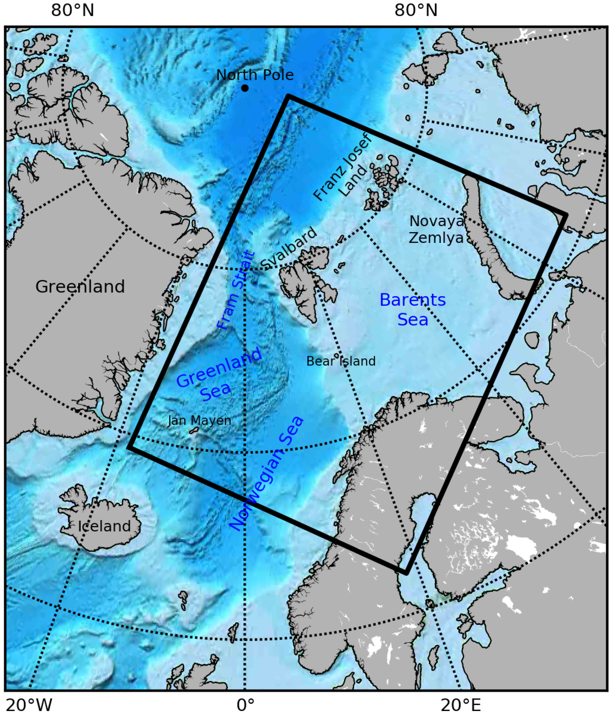
Figure 1 Study area: Barents-2.5km model domain shown by the thick rectangle.

The MDF of operational sea ice observations is performed for the sea areas around Svalbard, as shown by the thick rectangle in Figure 1. This is the model domain for the Barents-2.5-km operational ocean and sea ice forecast model at the Norwegian Meteorological Institute (Duarte et al., 2022; Röhrs et al., 2023), with the horizontal model grid resolution of 2.5 km. The Barents-2.5-km model does not contain ocean and sea ice information in the Baltic Sea. For consistency, we have also removed the sea ice in the Baltic Sea in this study. The fused sea ice observations will be further utilized for operational analysis and forecast.

2.1 SIC observations

There have been a large number of SIC observation through remote sensing (Kern et al., 2019). In this study, we use two high-resolution operational SIC products. One is the AMSR2 SIC data produced at the University of Bremen, and the other is sea ice chart from the Norwegian Meteorological Institute’s Ice Service (NIS). Figure 2 shows an example of the original SIC and standard deviation (SD) from these two data sets for 16/03/2022, as a typical winter sea ice condition in the Arctic.

Figure 2

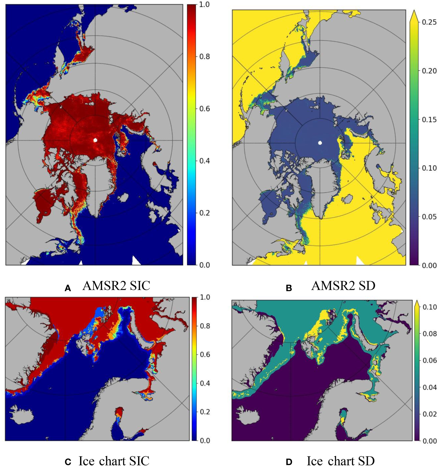
Figure 2 Original AMSR2 SIC and SD (A,B) and NIS ice chart (SIC and SD (C, D)) on 16/03/2022. The AMSR2 data is obtained from the University of Bremen, and the NIS ice chart is from the Norwegian Meteorological Institute.

2.1.1 AMSR2 SIC

The AMSR2 microwave radiometer onboard the GCOM-W1 satellite measures the microwave emission from the Earth, at a nominal incident angle of 55° and a swath width of 1,450 km. The AMSR2 SIC dataset we used here is version 5.4 with a grid resolution of 3.125 km, which utilizes the highest spatially resolving AMSR2 channels at 89 GHz (Melsheimer, 2019). It uses the same ARTIST sea ice (ASI) algorithm, as it was developed for the AMSR-E 89 GHz channel (Spreen et al., 2008). It has a higher spatial resolution than most other AMSR2 SIC datasets, but the atmospheric influence can be higher. The uncertainty is calculated following the same procedure in Spreen et al. (2008), where the overall error sums from three sources: the radiometric error from the bright temperature, the variability of the tie points, and the atmospheric opacity. The uncertainty is expressed in terms of SD. It is noted that this uncertainty does not account for individual, spatially varying atmospheric and surface effects as for example discussed in Rückert et al. (2023) and Rostosky and Spreen (2023).

2.1.2 NIS ice chart

Due to the large uncertainties in the PMRs for low SIC conditions (Cavalieri, 1994; Kern et al., 2019), we choose the NIS sea ice chart to mitigate the defect. The ice chart is produced based on manual interpretation of satellite data (Dinessen and Hackett, 2018), being a typical manually analyzed product. The ice charting employs a variety of satellite observations to obtain a more realistic SIE and MIZ. The main satellite data used are the weather-independent SAR data from RadarSat-2 and Sentinel-1. The analyst also uses visual and infrared data from METOP, NOAA, and MODIS in cloud-free conditions. These satellite data cover the charting area several times a day and are resampled to 1-km grid spacing. The NIS ice chart includes seven ice categories following the WMO sea ice nomenclature (WMO, 2014): fast ice (SIC = 10/10), very closed drift ice (9−10/10), closed drift ice (7−8/10), open drift ice (4−6/10), very open drift ice (1−3/10), open water (<1/10), and ice free (0). For practical use, a mean value is applied to denote the different ice categories in the ice chart. The uncertainty is approximated as the half of the range of the corresponding ice category, except being 0.01 for the fast ice. Apparently, this uncertainty is a very coarse estimate.

2.2 SIT observations

Remote sensing of SIT is much more difficult. There is thus far no sub-daily to daily SIT observation covering the whole Barents-2.5-km domain. The daily SMOS SIT has a high temporal resolution but with limitations of no observation north of 85°N and large uncertainties for SIT over 1 m. The weekly CS2SMOS SIT has better spatial coverage but has a limitation of weekly temporal resolution. In this study, we use these two products to generate a daily SIT data to cover the whole domain.

2.2.1 SMOS SIT

The SMOS SIT is retrieved from brightness temperature measured at the L-band (1.4 GHz) from ESA’s SMOS mission. The retrieval algorithm is based on a thermodynamic sea ice model and a three-layer radiative transfer model, which applies an iterative method to calculate SIT using bulk ice temperature and bulk ice salinity (Tian-Kunze et al., 2014). The SMOS SIT uncertainty is calculated based on the following factors: uncertainty of the measured brightness temperature, uncertainties of the auxiliary data sets (JRA55 reanalysis and sea surface salinity climatology), and the assumptions made for the radiation and thermodynamic models. The uncertainty increases rapidly with increasing SIT, and it is strongly recommended to use only data with a saturation ratio (provided in the dataset) less than 100% (Tian-Kunze et al., 2014). The data is gridded at the 12.5-km grid spacing on polar stereographic projection and is available from mid-October to mid-April in the Arctic. During winter seasons, the data is generated operationally by Alfred Wegener Institute (AWI), Germany, on daily basis with 24-h latency. SMOS SIT is obtained from ESA data collections (ESA, 2023a, version 3.3, accessed on 07.07.2023). As an example, the SMOS SIT and its SD on 16/03/2022 are shown in Figures 3A, B.

Figure 3

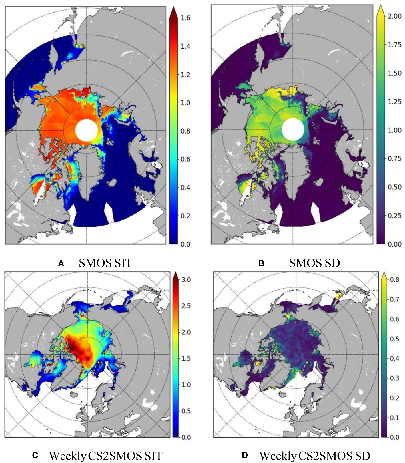
Figure 3 Original SMOS SIT and SD (A, B) and weekly CS2MSOS SIT and SD (C, D) on 16/03/2022. The weekly CS2SMOS SIT and SD are an estimate of weekly mean SIT and its SD during 13–19/03/2022. All the data are from AWI via ESA. The units are meters for both SIT and SD.

2.2.2 Weekly CS2SMOS SIT

The weekly CS2SMOS SIT is also produced by AWI and distributed via the ESA web portal (ESA, 2023b, version 2.05, accessed on 07.07.2023). CS2SMOS provides weekly SIT retrievals from merging daily SMOS thin SIT retrievals (Tian-Kunze et al., 2014) and SIT retrievals from CryoSat-2 (Hendricks and Paul, 2023), using an optimal interpolation approach (Ricker et al., 2017). The uncertainty of the CS2SMOS SIT is a natural part of the optimal interpolation. The data are projected onto the 25-km EASE2 Grid, based on a polar aspect spherical Lambert azimuthal equal-area projection. Figures 3C, D show the weekly CS2SMOS SIT and its SD on 16/03/2022, being an estimate of SIT and its SD during 13–19/03/2022.

3 MODF method

In this section, we describe the theoretical framework of MODF, which includes regridding, univariate multisensor optimal data merging (MODM), multivariate consistency check, and generation of new variables. The MODM has been used to optimally merge univariate multisensor observations (Wang et al., 2020), and it is here integrated as an important component of MODF.

3.1 Regridding

It is common that different remote sensing products have different projections and grids. Similarly, different applications would also have their own special projections and grids. For solving a certain desired application, we would thus need to remap the different satellite observations to the dedicated grid of the application. There are two common methods for such remapping: regridding and resampling. The essential difference between regridding and resampling lies in that regridding is performed on the grids, whereas resampling is performed on the points. Whether to use the regridding or resampling method depends mainly on the properties of the desired parameters. For example, if we need to remap the SIC, which is the fraction of the ice-covered area to the total area in a grid, then the regridding method shall be used. By contrast, if we need to remap the sea ice velocity field, then the resampling method shall be used at the grid points. In this case, the velocity inside a grid can be well-interpolated from the surrounding grid points, whereas using the grid-mean velocity is generally uncommon. In this study, for remapping the SIC and SIT, we use the regridding method, which can generally be separated in upgridding and downgridding.

3.1.1 Upgridding and downgridding

Upgridding refers to the process of regridding a source field to a finer-resolution destination field. This applies to both temporal and spatial fields. In this study, regridding of the weekly mean CS2SMOS SIT to daily would require upgridding in the temporal space, whereas both of the SMOS SIT (spatial resolution 12.5 km) and the CS2SMOS SIT (spatial resolution 25 km) would need upgridding of the two-dimensional spatial SIT to the Barents-2.5-km domain. Upgridding is generally performed through the interpolation technique, which is typically composed of nearest neighbor, linear, and cubic interpolations.

In contrast to the upgridding, downgridding is the process of regridding a source field to a coarser-resolution destination field. In the present study, the sea ice chart SIC has a spatial resolution of 1 km, and it would require downgridding to the relatively coarser resolution for the Barents-2.5-km domain. While the common interpolation methods, such as the nearest neighbor, linear, and cubic interpolation, are generally applicable for downgridding, conservative interpolation methods are preferred for some special cases which require high accuracy for tiny changes (Pletzer and Fillmore, 2015).

3.1.2 Effect of regridding on uncertainty

Due to the importance of observation uncertainty on data assimilation, it is essential to accurately determine the uncertainties of satellite observations due to regridding. To the authors’ knowledge, such an effect has not been considered thus far in the data assimilation community.

The effect of downgridding on the uncertainty may be derived as follows. Denote $x_1,x_2,\dots ,x_l$ as l independent observations with SDs ${\sigma }_1,{\sigma }_2,\dots ,{\sigma }_l,$ then the total is

$\begin{array}{ll}S=x_1+x_2+\cdots +x_l& (1)\end{array}$

which has variance

$\begin{array}{ll}\text{Var}(S)=\text{Var}(x_1)+\text{Var}(x_2)+\cdots +\text{Var }(x_l)=\sum _{k=1}^l{\sigma }_k^2.& (2)\end{array}$

The mean of these measurements $\overline{x}$ is simply given by

$\begin{array}{ll}\overline{x}=S/l.& (3)\end{array}$

The variance of the mean can then be calculated according to the Equations (1–3) such that

$\begin{array}{ll}\text{Var}(\overline{x})=\text{Var}(S/l)=\frac{1}{l^2}\text{Var}(S)=\frac{1}{l^2}\sum _{k=1}^l{\sigma }_k^2.& (4)\end{array}$

From Equation (4) we get the corresponding SD

$\begin{array}{ll}{\sigma }_{\overline{x}}=\frac{\sqrt{{\sum }_{k=1}^l{\sigma }_k^2}}{l}.& (5)\end{array}$

If the uncertainties of all the $l$ observations are equal, namely, ${\sigma }_k=\sigma$ then Equation (5) can be simplified as

$\begin{array}{ll}{\sigma }_{\overline{x}}=\frac{\sigma }{\sqrt{l}}.& (6)\end{array}$

Due to different manipulations of data, the effect of upgridding on the uncertainty may differ between temporally and spatially. For temporal upgridding such as the weekly CS2SMOS SIT into daily SIT, an inverse process to the downgridding shall be applied. If we assume that the daily SIT observations are independent on each other and their uncertainties are approximately equal, then the daily uncertainty σ can be estimated from the weekly uncertainty ${\sigma }_{\overline{x}}$ such that

$\begin{array}{ll}\sigma =\sqrt{l}{\sigma }_{\overline{x}},& (7)\end{array}$

where l = 7 in this case.

Equations (5–7) indicate the resulting uncertainty tends to decrease during downgridding and increase during upgridding. However, spatial upgridding of satellite observations may need special attention. It is noted that, for satellite products such as the AMSR2 SIC, SMOS SIT, and CS2SMOS SIT, their spatial resolutions may already be at the highest of the products. Therefore, upgridding does not produce more independent observations. As a consequence, the uncertainty would be unlikely to increase as significantly as the temporal upgridding. Further studies are needed to accurately determine the uncertainty variations for this situation. In this study, the uncertainties are assumed unchanged during the spatial upgridding.

3.2 MODM

Using the regridding method above, we can remap the individual sea ice observations to the dedicated area (here the Barents-2.5-km domain). These regridded multiple observations can be merged for the same univariate observations, using the MODM method (Wang et al., 2020). MODM here is used as a component of MODF. For self-containment, the main theoretical framework of MODM is described here with some minor modifications.

3.2.1 General solution

Consider a state variable vector x (column vector) such as SIC for a certain spatial domain such as the Barents-2.5-km domain (Figure 1), on a regular grid with the total grid number of n. Suppose we have m observations ${\text{x}}_k,k=1,\dots ,m$, for the true state vector ${\text{x}}_t$. These observations are assumed to be taken with different instruments, and their error vector associated with each measurement is ${ϵ}_k={\text{x}}_k-{\text{x}}_t$. We note that the observations are also assumed independent during the temporal regridding process in section 3.1.2. However, those observations are generally obtained using the same instrument but differ in the temporal distributions.

We assume that all the observations have been regridded and that all the error vectors are random, unbiased, and normally distributed. Thus, for the kth observation error vector, we have the mean $\mu =E({ϵ}_k)=0$ and covariance $R_k=E({ϵ}_k{ϵ}_k^T),$ where E denotes expectation operation and the superscript “T” denotes transpose. The probability density function (PDF) of such a error vector can be expressed as,

$\begin{array}{ll}f({ϵ}_k)=\frac{1}{{(2\pi )}^{1/2}|R_k{|}^{1/2}}\text{exp }\left(-\frac{1}{2}{ϵ}_k^T{R}_k^{-1}{ϵ}_k\right),& (8)\end{array}$

where $\left|R_k\right|$ denotes the determinant of $R_k$. If we further assume that the observation error vectors are not mutually correlated, that is, $E({ϵ}_j{ϵ}_k^T)=0$, when $j\ne k$, the PDF of the joint multivariate normal distribution for all the observation error vectors can be extended from Equation (8) and expressed as (Todling, 1999)

$\begin{array}{ll}f({ϵ}_1,{ϵ}_2,\cdots ,{ϵ}_m)=\prod _{k=1}^m\frac{1}{{(2\pi )}^{m/2}|R_k{|}^{1/2}}\text{exp}\left(-\frac{1}{2}{ϵ}_k^T{R}_k^{-1}{ϵ}_k\right),& (9)\end{array}$

where Π denotes the multiplication operator. It is thus easy to see from Equation (9) that the maximum likelihood estimate of $f({ϵ}_1,{ϵ}_2,\dots ,{ϵ}_m)$ is obtained by equivalently minimizing the following cost function

$\begin{array}{ll}J(x)=\sum _{k=1}^m{ϵ}_k^T{R}_k^{-1}{ϵ}_k=\sum _{k=1}^m{(x-x_k)}^T{R}_k^{-1}(x-x_k),& (10)\end{array}$

where the optimal estimate is considered as an approximate to the true value. Differentiate J(x) in Equation (10) against x and set it as 0,

$\begin{array}{ll}\frac{\partial }{\partial x}J(x)=\frac{\partial }{\partial x}\sum _{k=1}^m{(x-x_k)}^T{R}_k^{-1}(x-x_k)=2\sum _{k=1}^m{R}_k^{-1}(x-x_k)=0.& (11)\end{array}$

From Equation (11) we thus have the optimal estimate $x_o$ vector

$\begin{array}{ll}{x}_o={\left(\sum _{k=1}^m{R}_k^{-1}\right)}^{-1}\sum _{k=1}^m{R}_k^{-1}{x}_k,& (12)\end{array}$

and the optimal observation error vector

$\begin{array}{ll}{ϵ}_o=x_o-x_t={\left(\sum _{k=1}^m{R}_k^{-1}\right)}^{-1}\sum _{k=1}^m{R}_k^{-1}{ϵ}_k.& (13)\end{array}$

Since all the estimates are assumed as unbiased, normally distributed, and not mutually correlated, from Equation (13) we get the optimal observation error covariance

$\begin{array}{ll}R=E({ϵ}_o{ϵ}_o^T)={\left(\sum _{k=1}^m{R}_k^{-1}\right)}^{-1}.& (14)\end{array}$

The optimal estimate Equation (12) can be rewritten as

$\begin{array}{ll}{x}_o=R\sum _{k=1}^m{R}_k^{-1}{x}_k.& (15)\end{array}$

It is noted that the error covariance is symmetric and semi-positive definite. Consider the process for two data sets to be merged with the error covariance being R₁ and R₂, respectively. According to Equation (14), the merged data error covariance is

$\begin{array}{ll}\begin{array}{l}R={(R_1^{-1}+R_2^{-1})}^{-1}={[R_1^{-1}(R_1+R_2)R_2^{-1}]}^{-1}={R_2(R_1+R_2)}^{-1}{R}_1\\ \begin{array}{cc}& =R_1-R_1{(R_1+R_2)}^{-1}{R}_1=R_2-R_2{(R_1+R_2)}^{-1}{R}_2.\end{array}\end{array}& (16)\end{array}$

From Equation (16) and consider the properties of positive definite matrix, we see that the trace of R has the following property:

$\begin{array}{ll}tr(R)\le tr(R_1),tr(R_2).& (17)\end{array}$

Equation (17) indicates that the sum of the error variance of merged data is no larger than any of the individual observations. For more observations, we can use this analysis successively. With more and more observations, the sum of the merged error variance will become smaller and smaller. Therefore, the MODM process is to combine multiple observations with reducing uncertainty and increasing confidence. In addition, the MODM method can significantly reduce the computational cost and storage for data assimilation, as assimilating the merged multisensor observations is equivalent to assimilating the individual observations concurrently (Wang et al., 2020).

3.2.2 Simplification of MODM

In recent years, more and more sea ice remote sensing observations begin to provide local variance or SD as a measure of uncertainty (Tian-Kunze et al., 2014; Ricker et al., 2017; Tonboe et al., 2016; Lavergne et al., 2019). Accordingly, the MODM method may be simplified by further assuming that each observation error vector is spatially uncorrelated. In this case, the kth error covariance, R_k (Equation 14), becomes

$\begin{array}{ll}{R}_k=E({ϵ}_k{ϵ}_k^T)=\left[\begin{array}{ccccc}{\sigma }_{1,k}^2& & & & \\ & \ddots & & & \\ & & {\sigma }_{j,k}^2& & \\ & & & \ddots & \\ & & & & {\sigma }_{n,k}^2\end{array}\right],& (18)\end{array}$

where ${\sigma }_{j,k}$ is the SD of the kth observation at the jth grid, where $k=1,\dots ,m$ and $j=1,\dots ,n$. In this case, the error covariance (Equation 14) and the optimal estimate (Equation 15) of the multisensor observations can be expressed on individual grid (Equation 18),

$\begin{array}{ll}{\sigma }_j={\left(\sum _{k=1}^m{\sigma }_{j,k}^{-2}\right)}^{-1/2},& (19)\end{array}$

$\begin{array}{ll}{x}_j={\sigma }_j^2\sum _{k=1}^m{x}_{j,k}{\sigma }_{j,k}^{-2},& (20)\end{array}$

where $j=1,\dots ,n$ is the grid ordinal number. Equations (19) and (20) are used in this study for MODM of SIC and SIT.

3.3 Multivariate consistency

Due to the inherent defect of PMRs in the observation of low SIC, it is common that some of the sea ice close to the SIE is underestimated or even removed by weather filters. For such situations, the SIC can be improved by using a sea ice chart which is based on a large variety of sea ice satellite observations. However, there is no similar observations yet for the SIT; therefore, a reasonable treatment must be presented to mitigate the deficiency. One such solution is the empirical relationship between SIC and SIV for thin sea ice (Fritzner et al., 2018), which is based on a non-linear regression for SIT up to 0.4 m. The corresponding SIT can thus be easily obtained via SIT = SIV/SIC as follows (Wang et al., 2023):

$\begin{array}{ll}{h}_m=0.02e^{2.8767a_m},& (21)\end{array}$

where a and h denote SIC and SIT, $h_m$ denotes the missing SIT, and $a_m$ denotes the SIC in the areas where a > 0 but the original SIT h_{0 =} 0. It is noted that the valid SIC range in Equation (21) is also slightly extended such that $a_m\in (0,1]$ (Wang et al., 2023). The corresponding uncertainty for this newly created SIT $h_m$ can be estimated through the Gaussian propagation of uncertainty together with Equation (21) such that

$\begin{array}{ll}{\sigma }_{h_m}=2.8767h_m{\sigma }_{a_m}.& (22)\end{array}$

Thus, the overall fused SIT uncertainty can be approximated as

$\begin{array}{ll}{\sigma }_h={({\sigma }_{h_m}^2+{\sigma }_{h_0}^2)}^{1/2},& (23)\end{array}$

where ${\mathrm{\sigma h}}_0$ is the SD of the original SIT $h_0$.

3.4 Generation of new variables

One of the main purposes of the MDF is to generate new variables that are not possible with any single variables. Here, we show from the combination of SIC and SIT, we can obtain a series of more robust, accurate, and complete description of the sea ice conditions.

3.4.1 Sea ice volume

Sea ice volume (SIV) is not directly observed, and there has been no studies to estimate the SIV uncertainty. Here, we deduce the formulation for SIV (V) based on the observed SIC (a) and SIT (h) and their SDs ${\sigma }_a$and ${\sigma }_h$. It is generally reasonable to assume that a and h are two independent random variables; thus, V can be simply expressed as

$\begin{array}{ll}V=ha,& (24)\end{array}$

and its SD can be calculated according to the variance of the products (Goodman, 1960)

$\begin{array}{ll}{\sigma }_V={(h_{mean}^2{\sigma }_a^2+a_{mean}^2{\sigma }_h^2+{\sigma }_a^2{\sigma }_h^2)}^{1/2},& (25)\end{array}$

where the subscript “mean” denotes the mean values of SIC and SIT. It is noted that Equation (25) is the exact variance of products, whereas the Gaussian propagation of uncertainty is an approximate solution after neglecting high-order derivatives and cross-correlated terms.

3.4.2 Sea ice edge

According to the World Meteorological Organization (WMO, 2014), SIE is defined as the demarcation at any given time between open sea and sea ice of any kind. It can generally be separated into two types: compacted and diffuse. The compacted SIE refers to the close and clear-cut SIE, which is compacted by wind or current, usually on the windward side of an area of drift ice. The diffuse SIE refers to the poorly defined SIE, which has an area of dispersed ice, usually on the leeward side of an area of drift ice. In practical usages, SIE is often defined as the demarcation where SIC = 0.15 in the sea ice and climate modeling communities. By contrast, it is often defined as the demarcation where SIC = 0.1 in the sea ice charting community, such as the NIS ice chart (https://cryo.met.no) and US National Ice Center (NIC) ice chart (https://usicecenter.gov/Products). Wang et al. (2023) argue that choosing SIC = 0.1 as the demarcation for SIE has several benefits. Most importantly, it has a clear physical representation that distinguishes open water (SIC<1/10) and very open drift ice (SIC in 1–3/10). In addition, it provides a consistent definition for the joint sea ice modeling and charting community. In this study, we also use SIC = 0.1 as the demarcation for SIE.

3.4.3 Marginal ice zone

MIZ is generally referred to the transition region from open water to dense pack ice that is affected by open ocean processes (Wadhams, 1986; Johannessen et al., 1987), although its accurate definition is still under intensive discussion from different viewpoints and concerns. Typical MIZ conditions are found along the southern edges of the ice pack in the Bering, Greenland, and Barents seas, in the Baffin Bay, and along the complete northern edge of the Antarctic ice cover (Røed and O’Brien, 1983). There have been several definitions for the MIZ. The most widely used one is solely based on SIC, commonly defined as the region where SIC ∈ [0.15,0.8]. In order for a consistent definition in both ice charting and sea ice modeling, the MIZ is here defined as follows

$\begin{array}{ll}{\text{MIZ}}_t=\text{regions where }a\in [0.1,0.8]& (26)\end{array}$

where a is the SIC, and the subscript “t” denotes traditional. This traditional definition has been applied in a variety of applications, such as sea ice charting (e.g., the NIC ice chart), satellite observations (e.g., Strong, 2012; Liu et al., 2019a), sea ice modeling (e.g., Wang et al., 2023), primary productions (e.g., Barber et al., 2015), marine ecosystems (e.g., Wassmann, 2011; Arrigo, 2014), and ship navigation (e.g., Palma et al., 2019).

The above traditional definition of MIZ provides a reasonable quantification of the MIZ extent. However, it is often inadequate for a detailed description of MIZ dynamics (see Bennetts et al., 2022 and references therein). In such cases, the effect of waves must be taken into consideration. To observe the dynamical MIZ, Dumont (2022) suggests three approaches, in which sea ice displays vortical motions, wavy motion, or a dominant floe size less than an upper value (in the order of 200 m–500 m). We comment that the vortical and wavy motions are generally unstable features, so they are not proper for a consistent determination of the dynamical MIZ. For example, the ice eddies or waves in the ice could be temporally diminished in the MIZ whereas the ice floes remain unchanged. In such cases, the extent of the MIZ should remain according to the floe size method, rather than vanished according the other two methods. Therefore, the floe size method appears to be the most appropriate method for observing the dynamical MIZ.

The sea ice floe size is not operationally observed for the sea areas around Svalbard. As an alternative, we approximate the dynamical MIZ using combined SIC and SIT based on the model results from a coupled wave and ice model (Dumont et al., 2011),

$\begin{array}{ll}{\text{MIZ}}_d=\text{regions where}\{\begin{array}{l}a\in [0.1,0.85], h\le 2.0\hfill \\ \text{or}\hfill \\ a>0.85, h\le 10.5-10a\hfill \end{array}& (27)\end{array}$

where a and h denote SIC and SIT and the subscript “d” denotes dynamical. The lower SIC bound of 0.1 is here used to be consistent with the SIE. Compared with the traditional ${\text{MIZ}}_t$ the dynamical ${\text{MIZ}}_d$ also includes part of the very close drift ice, although the SIT tends to be thinner with increasing SIC.

It is noted that the dynamical MIZ formulation Equation (27) is solely based on the simulation results at the Fram Strait of a 1D coupled wave-ice model (Dumont et al., 2011). Its accuracy and validity for other sea areas needs further verification. The upper SIC bound of 0.85 is used here to be consistent with the simulation results (Dumont et al., 2011), which is slightly larger than the traditional upper bound of 0.8 (see Equation 26). This difference can partly be explained by the constraint h ≤ 2.0 in Equation (27). For h > 2.0 m, the upper SIC bound is supposed to become lower than 0.85 and approach to 0.8.

4 Results

In this section, we fuse the AMSR2 SIC, NIS ice chart, SMOS SIT, and weekly CS2SMOS SIT to generate a united, consistent, and multifaceted daily description of the sea ice for the Barents-2.5-km area. The corresponding data are available at https://doi.org/10.5281/zenodo.10726427.

4.1 MODF of SIC

The original SIC and their SD of the AMSR2 and NIS ice chart are shown in Figure 2. The AMSR2 covers the whole northern hemisphere, whereas the NIS ice chart only covers the European Arctic. The regridding of the SIC and SD is performed using the nearest neighbor interpolation method. The effects of spatial regridding on the uncertainties are ignored. The regridded SIC and SD in the Barents-2.5-km domain are shown in Figures 4A–D. While the overall sea ice distributions are similar, there are noticeable differences between the AMSR2 SIC and the NIS ice chart. One notable difference is the very open drift ice (SIC 1–3/10) north of Svalbard and Franz Josef Land, which is clearly recognized in the ice chart, but identified as ice free (SIC = 0) in the AMSR2 SIC. This is the shortcoming commonly in the PMWs, which have low capabilities in accurately determining low SIC (Cavalieri, 1994; Kern et al., 2019). It is noted that such high uncertainty is very well described in the AMSR2 product (Figure 4B). Application of a large variety of remote sensing products in the ice charting effectively improves the identification of the very open drift ice. Another prominent difference is the fine features within the very close drift ice (9–10/10), which are clearly seen in the AMSR2 SIC (Figures 4A, B), but missing in the ice chart (Figures 4C, D). This is one shortcoming in the manual ice charting, as such features could often be ignored by the analyst.

Figure 4

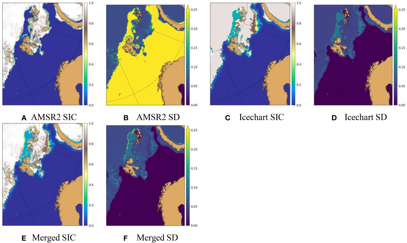
Figure 4 SIC and its SD on 16/03/2022: regridded AMSR2 (A, B), ice chart (C, D) and merged (E, F).

In order to compensate for the missing features in the very close drift ice in the ice chart, one feasible method is to increase the corresponding uncertainty. In this study, we have set the SD for the very close drift ice in the ice chart as 0.3 during the SIC MODM. This seems to be a reasonable estimate based on the merged SIC and its SD (Figures 4E, F). Merging of the AMSR2 SIC and ice chart SIC follows Equations (19) and (20). On the whole, the merged SIC SD resembles the NIS ice chart SD (cf. Figures 4F, D), due mainly to the much higher uncertainties in the AMSR2 open water and ice free areas (Figure 4B). The fine features in the AMSR2 are very well maintained in the merged SIC (cf. Figures 4A, E). Similarly, SIC (lower). The data in the Baltic Sea have been removed according to the Barents-2.5-km model setting. The very open drift ice in the north of Svalbard and Franz Josef Land and in the northeast Barents Sea is very well preserved (cf. Figures 4C, E).

there is a noticeable difference in the Arctic central pack ice in the AMSR2 SIC and ice chart, particularly north of the very open drift ice between Svalbard and Franz Jozef Land. It was observed as very close drift ice in the ice chart but identified as ice free in the AMSR2 SIC. This difference is most probably caused by the different time of the observations. The relatively large SD also suggests a strong diurnal variation there (Figure 4F). The merged SIC along this high SD area is around 0.45 (Figure 4E), being a weighted average between the AMSR2 SIC and the ice chart SIC.

4.2 MODF of SIT

The MODF of SIT includes two parts. The first part is the MODM of daily SMOS SIT and weekly CS2SMOS SIT to form a merged daily CS2SMOS SIT, and the second part is a consistency check of the merged daily CS2SMOS SIT with the merged SIC.

4.2.1 MODM of SIT

The MODM of SIT follows much of the same procedure for the SIC. The original SIT and SD for the daily SMOS and weekly CS2SMOS are shown in Figure 3, both covering the whole northern hemisphere, with the spatial resolutions of 12.5 km and 25 km, respectively. These two SIT products are firstly upgridded to the Barents-2.5-km domain using the nearest-neighbor interpolation (Figures 5A–D). For clarity purposes, the uncertainties have both remained unchanged during the regridding. It can be seen that there are considerable differences in these two products (Figure 5). The SMOS SIT has a relatively large data hole around the North Pole. The uncertainty increases rapidly when the observed SIT is over 1 m, as can also be seen in Figures 5A, B. By contrast, the weekly CS2SMOS SIT has a full coverage of the whole domain, with the SIT generally up to 3 m (Figure 5C). The CryoSat-2 SIT has large uncertainties when it is thinner than 1 m (Ricker et al., 2017), and the weekly CS2SMOS SIT effectively reduces the overall uncertainty by combining the CryoSat-2 SIT and the SMOS SIT.

Figure 5

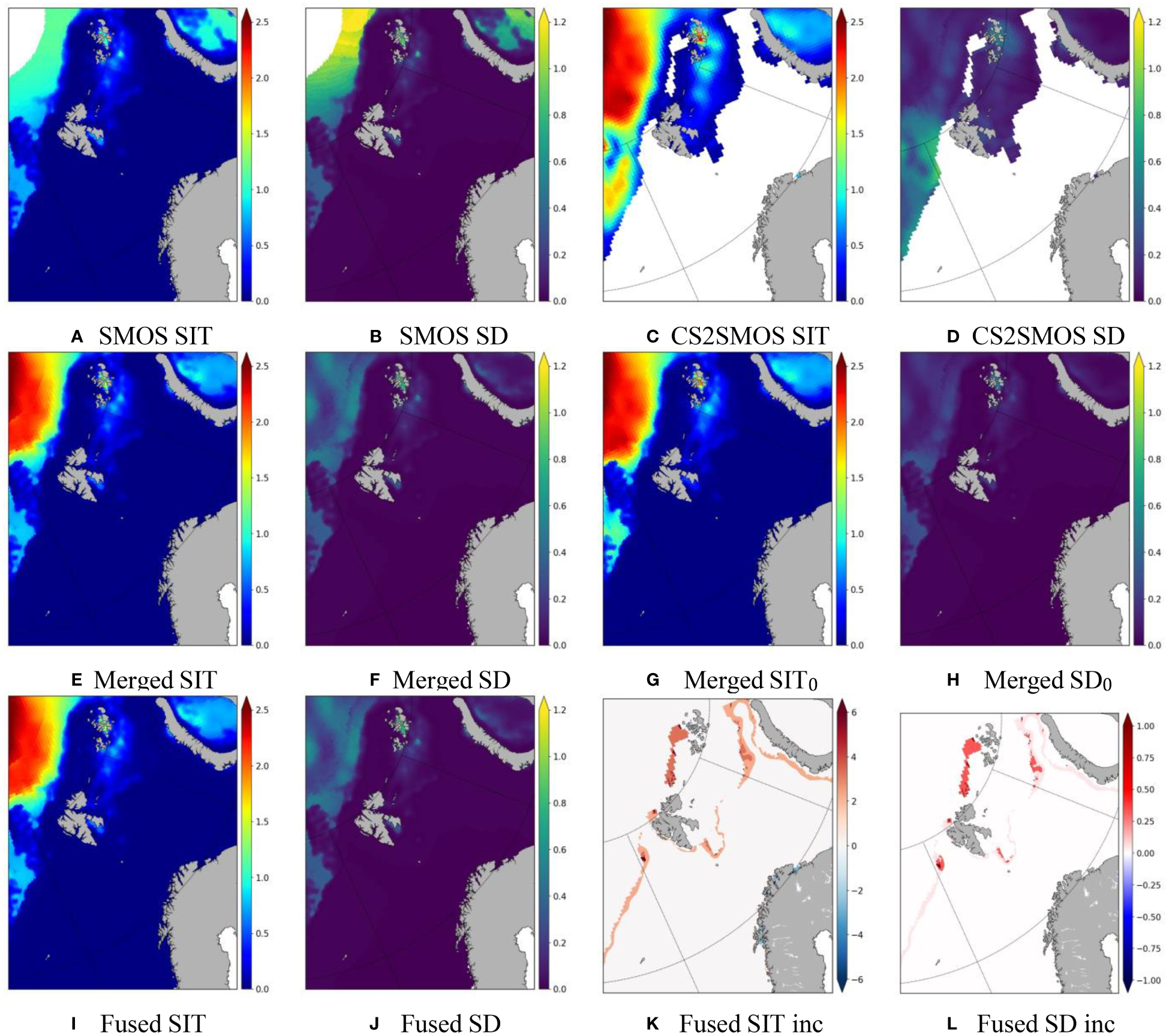
Figure 5 SIT and its SD on 16/03/2022: regridded daily SMOS SIT (A, B), regridded weekly CS2SMOS SIT (C, D), merged daily CS2SMOS SIT with temporal upgridding effect (E, F), merged daily CS2SMOS SIT without temporal upgridding effect (G, H), fused SIT and increment (I–L). The fused increments denote the SIT and SD differences of fused–merged. The units of the SIT and SD are m; the units of the increments are cm.

It is noteworthy that the weekly CS2SMOS SIT is a weekly mean; therefore, it can be biased when used for daily purposes. One such case can be seen in the north Greenland Sea, west of Svalbard (cf. Figures 5A, C). We can see that the thin SMOS SIT there is generally approximately 0.5 m (Figure 5A), whereas the weekly CS2SMOS SIT is mostly over 1 m (Figure 5C). This discrepancy is due mainly to the weekly average of the CryoSat-2 SIT and SMOS SIT over the whole week, in which both thin and thick ice drifting before and after the day are accounted for. Therefore, for daily usage, a more accurate estimate of the thin ice should be closer to the daily SMOS SIT. It is apparent that assimilation of such weekly SIT as a daily data would introduce considerable systematic bias.

The merged daily CS2SMOS SIT and SD with and without the temporal upgridding effect are shown in Figures 5E–H, in which the subscript “0” denotes no temporal upgridding effect. It is seen that the merged SD is noticeably larger than SD₀ (cf. Figures 5F, H), particularly for the larger SIT areas in the Arctic Ocean and Greenland Sea. By contrast, the merged SIT is slightly lower than SIT₀ (cf. Figures 5E, G). On the whole, the merged daily CS2SMOS SIT is closer to the SMOS SIT, whereas the SIT₀ is closer to the weekly CS2SMOS SIT, although the thick ice in both SIT and SIT₀ are close to the weekly CS2SMOS SIT.

The merged thin SIT to the west of Svalbard is very close to that in the SMOS SIT (cf. 5e and 5a), showing a successful merging as discussed above. However, the overall distributions of the merged SIT and SIT₀ in the Kara Sea (east of Novaya Zemlya) appear much closer to the weekly CS2SMOS ST than the SMOS SIT, although more similarities are seen to the SMOS SIT when considering the temporal upgridding effect (cf. Figures 5A, C, E, G). Since the SIT there is generally approximately 0.7 m–0.9 m, a reasonable result would be that the merged SIT is closer to the SMOS SIT rather than the weekly CS2SMOS SIT. The most probable reason for the discrepancy is that the uncertainty there in the weekly CS2SMOS SIT (Figure 5D) is underestimated. This is confirmed by the weekly CS2SMOS SIT SD, which is generally less than 0.06 m in this area (Figure 5D). It is much lower than the SMOS SIT SD (generally approximately 0.7 m as shown in Figure 5B), even after the temporal downgridding from daily to weekly. A further refinement of the weekly CS2SMOS SIT uncertainty would be highly desirable.

4.2.2 Check of consistency

The fused SIT and its SD are generally similar to the merged ones in much of the domain (cf. Figures 5I, J, E, F). Their differences are calculated according to Equations (22) and (23), and shown in Figures 5K, L. The differences are mainly located near the SIE, with the additional thin SIT in several cm and additional SD below 1 cm. Such a supplementary effectively overcomes the shortcoming of the PMRs, thus generating a more consistent and accurate observation of the SIE and MIZ compared with the merged SIT and SD. The application of the ice chart also removes some coastal sea ice along the mainland Norway (Figures 5K, L).

4.3 MODF of SIV

Direct observations of SIV and its SD are so far not feasible, so they are calculated according to Equations (24) and (25) with the observed SIC and SIT. Since SIC is a dimensionless variable, the unit of SIV is the same as that of SIT, representing the mean SIT of the concerned grid. On the whole, the SIV resembles the fused SIT (cf. Figures 6A, 5I for reference). This is partly due to the fact that the majority of the sea ice is very close drift ice (Figure 4E), with the SIC close to 1. Different from the SIV, its uncertainty is nonlinearly dependent on the SIC, SIT, and their uncertainties (Equation 20). The overall distribution of the SIV SD is also close to the SIT SD (Figures 6B vs. 5J).

Figure 6

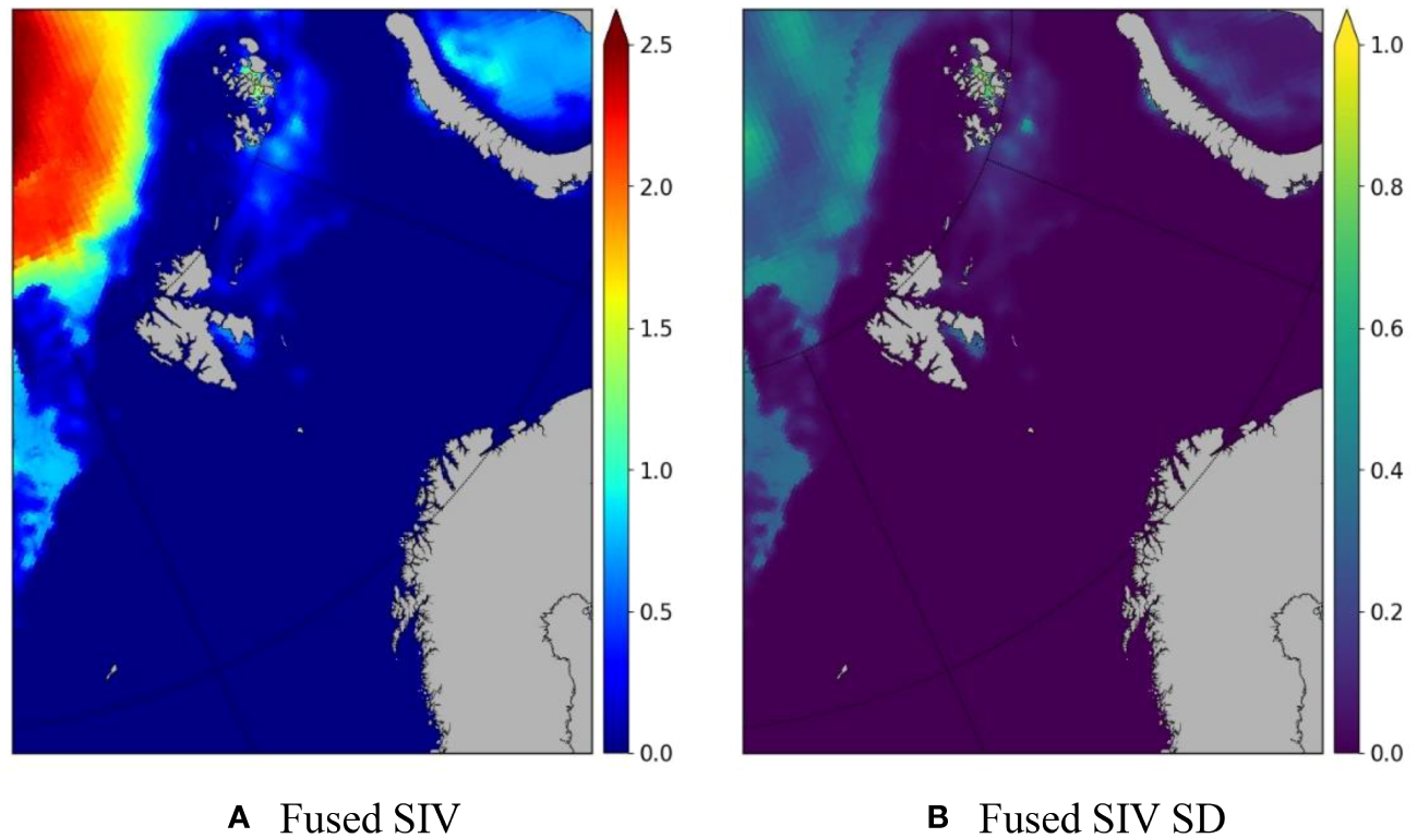
Figure 6 Fused SIV (A) and its SD (B) per m² on 16/03/2022. The units are meters for both SIV and its SD.

4.4 SIE and MIZ

SIE and MIZ are byproducts of operational sea ice observations. In this study, we focus mainly on their distributions; their uncertainties are not estimated. As an example, Figure 7 shows the MIZ distributions on 16/03/2022. The traditional MIZ_t is solely based on SIC (Equation 26), whereas the dynamical MIZ_d is based on a combination of SIC and SIT (Equation 27). In this study, we have set the SIE as the lower bound of MIZ, being the demarcation where SIC = 0.1. The extra condition of SIT<2.0 m for MIZ_d in Equation (27) generally has a minor effect on the SIE. As can be seen from Figure 7, when using the same data sources, there are no noticeable differences in the SIE between the MIZ_t and MIZ_d.

Figure 7

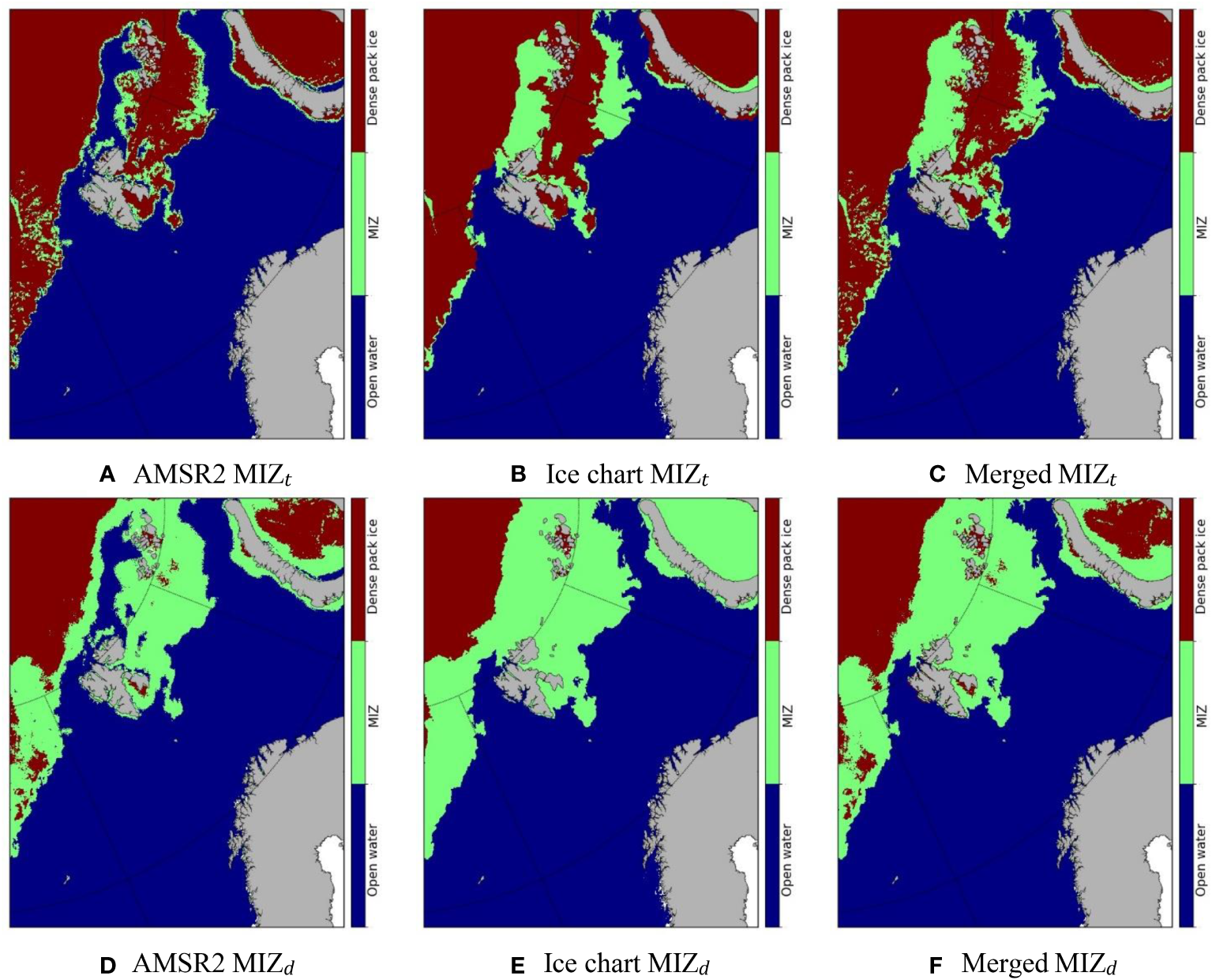
Figure 7 MIZ distribution on 16/03/2022: traditional MIZ_t from (A) AMSR2, (B) NIS ice chart, and (C) merged SIC, and dynamical MIZ_d from (D) AMSR2, (E) NIS ice chart, and (F) merged SIC. For the determination of MIZ_d, the fused SIT are used in all the three cases (D–F).

There are significant differences in the MIZ_t and MIZ_d. The most prominent difference is the very close drift ice in the Barents Sea, which was identified as dense pack ice in the MIZ_t (Figures 7A–C), but as MIZ in the MIZ_d (Figures 7D–F). Such difference also occurs in the Kara Sea and Greenland Sea. The SIT in these areas are generally less than 0.8 m (Figure 5E). This indicates that either lower SIC or low SIT can contribute to the MIZ_d.

Different data sources have a strong impact on the determination of MIZ. This can be clearly seen in the three traditional MIZ_t (Figures 7A–C). As mentioned in section 4.1, a large patch of very open drift ice in the ice chart north of Svalbard and Franz Josef Land (Figure 7B) was identified as open water in the AMSR2 MIZ_t (Figure 7A). By contrast, some fine features identified by the AMSR2 SIC were missing in the ice chart (cf. Figures 7A, B). Similar to the merging of SIC (Figure 4), the merged MIZ_t also includes the very open drift ice identified in the NIS ice chart and the fine features identified in the AMSR2 SIC. It remains to be further discussed whether such fine features should be included in the MIZ_t.

The MIZ_d is seen very sensitive to the SIC. A large part of the sea ice in the Kara Sea is identified as dense pack ice according to the AMSR2 SIC (Figure 7D), whereas the ice in the whole Kara Sea is classified as MIZ according to the ice chart (Figure 7E), both using the fused SIT (Figure 5F). Since we use the same SIT for determining the MIZ_d, the differences are mainly caused by the difference in the SIC. The SIC in the ice chart is 0.95, whereas the SIC in the AMSR2 is very close to 1 for the dense pack ice region. Similar results occur in the Greenland Sea, where some small patches of the very close sea ice are identified as dense pack ice (Figures 7D, F), whereas it is almost all identified as MIZ when using the NIS ice chart (Figure 7E). This indicates that the NIS SIC is generally of coarse resolution in the SIC space and would be insufficient for the accurate determination of the MIZ_d. It is noted that the current MIZ_d is parameterized based on the simulations from one-dimensional wave-ice coupled model (see Equation 27) at the Fram Strait. Its feasibility and reliability remains to be further verified for the whole Barents-2.5km area.

5 Discussion

5.1 Evaluation

No formal evaluation is performed in this study. This is partly due to the fact that all the data are from observations, which are so far among the best available data for sea ice observations. In such a case, it is very difficult to find better observation data for evaluation, and it is generally of limited values to evaluate the results with lower-quality data (Wang et al., 2023).

Nevertheless, the natural limitations of the observations can help justify the advantage of the MODF, as can be clearly seen from the results. For example, for the MODF of SIC (Figure 4), it is well known that the passive microwave remote sensing products have a general shortcoming when applying for low SIC conditions (e.g., Cavalieri, 1994; Spreen et al., 2008; Kern et al., 2019), whereas the manually analyzed sea ice chart tends to ignore some fine features within the ice pack. Such deficiencies are almost perfectly mitigated in the merged SIC. Compared with the original AMSR2 SIC and NIS ice chart, the merged SIC clearly preserves the fine features in the AMSR2 SIC and the very open drift ice observed in the ice chart (Figure 4).

Similarly, for the MODF of SIT (Figure 5), the SMOS SIT only covers a limited area with very large uncertainties for SIT over 1 m, whereas the weekly CS2SMOS SIT only provides a weekly mean, which is generally not adequate for accurate daily description, particularly for sea ice under rapid movement or thermal growth. In the present case, the weekly CS2SMOS SIT tends to overestimate a patch of daily SIT in the Greenland Sea, which is corrected by merging the SMOS SIT. The SIT is further improved via the multivariate consistency check. With the improvements in both SIC and SIT, it is straightforward to know that the fused SIV is improved.

5.2 Observation uncertainties

As shown in Equations (12, 19, and 20), the merged value is strongly dependent on the original observation uncertainties. Therefore, accurate determination of the original observation uncertainties is critical to the final merged and fused results. In this study, the SD of the AMSR2 SIC for the open water is approximately 0.25, which results from three sources (Spreen et al., 2008). Such a high value correctly depicts the large uncertainties of PMRs for low SIC conditions (Cavalieri, 1994; Kern et al., 2019). Similarly, we used a large uncertainty of 0.3 for the very close drift ice in the NIS ice chart to account for the often neglected fine features. On the whole, such high uncertainties provide an important foundation for the successful SIC merging.

One special deficiency is noteworthy in the sea ice satellite remote sensing: the uncertainty is often underestimated. For the SIC merging case mentioned above, we have also tested using low uncertainties for the low AMSR2 SIC and the NIS very close drift ice. In such a case, the resulting merged SIC captures neither the very open drift ice north of Svalbard and Franz Josef Land nor the fine features observed in the AMSR2 SIC. Similar underestimate occurs in the merging of SIT in the Kara Sea, where the weekly CS2SMOS SIT is approximately 0.7 m with an SD below 0.06 m (Figure 5). The resulting merged daily CS2SMOS SIT tends to be closer to the weekly mean rather than the daily SMOS SIT. A further study of the case would be highly desirable.

5.3 Further expansion of the observations

In this study, we have focused on the fusion of SIC, SIT, and SIV for the operational purpose. This is due to the fact that for marine operations such as the sea area around Svalbard, SIC, SIT, SIE, and MIZ are the most important sea ice parameters for safe operations. As can be seen in the analysis, SIE and MIZ can be deduced from the observed SIC and SIT. SIV can also obtained from the combination of SIC and SIT, which is important for sea ice modeling and assimilation, as well as for overall sea ice mass estimate. In general, sea ice velocity, temperature, and age are also important for safe operations but considered as secondary. In particular, initial sea ice velocity would soon lose its inertia in several hours. Therefore, accurate prediction of sea ice velocity would strongly rely on the initial SIC and SIT, as well as the model quality rather than its initial velocity. Nevertheless, these parameters can be included if they are necessary.

Accurate and consistent description of sea ice is an important part of climate studies. A comprehensive set of sea ice variables, such as SIC, SIT, SIV, sea ice drift, sea ice age, melt pond fraction, and sea ice surface albedo, would be valuable for climate analysis, simulation, evaluation, and prediction. There are emerging discussions on such needs (e.g., Lavergne et al., 2022; Sandven et al., 2023). The present framework can be naturally expanded with more variables, longer time scale, and larger spatial coverage, thus generating united, consistent, and multifaceted climate data sets.

6 Conclusions

Sea ice is one of the most severe threats to the marine operations around Svalbard. With the continuous increasing of marine activities around Svalbard, monitoring and prediction of sea ice is urgently needed for safe and sustainable development. In this study, we introduced a new MDF method, MODF, and applied it to fuse the operational sea ice observations around Svalbard, with the focus on the SIC and SIT. The results will be further used in the operational Barents-2.5-km model (Duarte et al., 2022; Röhrs et al., 2023) at the Norwegian Meteorological Institute.

The overall MODF method includes regridding, univariate MODM, multivariate consistency check, and generation of new variables. Individual SIC or SIT operational products have their own spatial and temporal coverages and resolutions, which are often different from the concerned applications. Regridding (upgridding or downgridding) is therefore needed to remap such products to the desired coverage and resolution. In this study, we have used a simple nearest neighbor interpolation method for both upgridding and downgridding. While the uncertainty would be theoretically altered during the regridding, it is only considered during the temporal upgridding of the weekly CS2SMOS SIT in this study. Further studies are desirable to investigate the exact regridding effect on the uncertainties.

The univariate MODM is here used to merge multisensor observations of the same variable following Wang et al. (2020). The advantage of the MODM is to extract the most confident parts of the observations to form a refined variable. In this study, the NIS ice chart has a higher capability to accurately depict the low SIC area, whereas the AMSR2 SIC has the advantage to describe the SIC more continuously and accurately away from the low SIC area. Similarly, the weekly CS2SMOS SIT has low uncertainty for thick sea ice, whereas SMOS SIT has low uncertainty for thin sea ice. Merging of SMOS SIT and weekly CS2SMOS SIT thus provides a refined daily SIT observation for both thin and thick sea ice. The univariate MODM therefore provides a very efficient method to combine different sensors for observing the same sea ice variable.

The multivariate MODF is an extension of the univariate MODM, from single variable to multiple variables. For each variable, the univariate MODM is firstly applied to form a refined variable. A further combination of the multiple variables is performed during the multivariate MODF via consistency checks. Such consistency checks can supplement extra information for the observations (Figure 5). In addition, new variables such as SIV, SIE, and MIZ can be generated, which provide extra insight into the sea ice observations.

The present study provides a fundamental framework for managing multivariate multisensor observations. The main focus here has been on the data fusion of operational sea ice observations (SIC, SIT, SIV, and their uncertainties), which are the most important for operational sea ice monitoring and predictions. It is straightforward to extend the present data sets to include more variables for climate studies, such as sea ice age, sea ice drift, melt pond fraction, and snow depth (Lavergne et al., 2022; Sandven et al., 2023). The MODF is also applicable for other environmental observations in order to form a consistent, multifaceted, and more robust and accurate description.

Data availability statement

The AMSR2 SIC is available at https://seaice.uni-bremen.de/data/amsr2/. The NIS ice chart is available at https://doi.org/10.48670/moi-00128. The SMOS SIT and the weekly mean CS2SMOS SIT are available at ftp://smos-diss.eo.esa.int/SMOS/. The corresponding data regridded on the Barents-2.5-km grid and their merged and fused data are available at https://doi.org/10.5281/zenodo.10726427.

Author contributions

KW: Conceptualization, Formal analysis, Funding acquisition, Investigation, Methodology, Project administration, Software, Validation, Visualization, Writing – original draft, Writing – review & editing. CW: Formal analysis, Funding acquisition, Investigation, Writing – review & editing. FD: Writing – review & editing, Data curation, Investigation. GS: Data curation, Investigation, Writing – review & editing. RR: Data curation, Investigation, Writing – review & editing. XT-K: Data curation, Investigation, Writing – review & editing.

Funding

The author(s) declare financial support was received for the research, authorship, and/or publication of this article. This study was supported by the Norwegian FRAM Flagship program project SUDARCO (grant No. 551323), the Nordic Council of Ministers project NOCOS DT (grant no. 102642), and the Norwegian Research Council project 4SICE (grant no. 328886).

Conflict of interest

The authors declare that the research was conducted in the absence of any commercial or financial relationships that could be construed as a potential conflict of interest.

Publisher’s note

All claims expressed in this article are solely those of the authors and do not necessarily represent those of their affiliated organizations, or those of the publisher, the editors and the reviewers. Any product that may be evaluated in this article, or claim that may be made by its manufacturer, is not guaranteed or endorsed by the publisher.

References

AMAP (2017). Adaptation Actions for a Changing Arctic (AACA) - Barents Area Overview report, Arctic Monitoring and Assessment Programme (AMAP) (Oslo, Norway: AMAP), pp. 24. https://www.amap.no/documents/doc/adaptation-actions-for-a-changing-arctic-aaca-barents-area-overview-report/1529

Google Scholar

Arrigo K. R. (2014). Sea ice ecosystems. Annu. Rev. Mar. Sci. 6, 439–467. doi: 10.1146/annurev-marine-010213-135103

CrossRef Full Text | Google Scholar

Barber D., Hop H., Mundy C., B. E., Dmitrenko I., Tremblay J., et al. (2015). Selected physical, biological and biogeochemical implications of a rapidly changing arctic marginal ice zone. Prog. Oceanogr. 139, 122–150. doi: 10.1016/j.pocean.2015.09.003

CrossRef Full Text | Google Scholar

Bennetts L., Bitz C., Feltham D. L., Kohout A. L., Meylan M. H. (2022). Theory, modelling and observations ofmarginal ice zone dynamics: multidisciplinary perspectives and outlooks. Phil.Trans.R.Soc 380, 20210265. doi: 10.1098/rsta.2021.0265

CrossRef Full Text | Google Scholar

Cavalieri D. J. (1994). A microwave technique for mapping thin sea ice. J. Geophys. Res. 99, 12561–12572. doi: 10.1029/94JC00707

CrossRef Full Text | Google Scholar

Dinessen F., Hackett B. (2018). Product user manual for regional high resolution sea ice charts Svalbard region (Ramonville-Saint-Agne, France: EU Copernicus Marine Service), pp. 16. Available at: http://marine.copernicus.eu/documents/PUM/CMEMS-OSI-PUM-011-002.pdf

Google Scholar

Duarte P., Brændshøi J., Shcherbin D., Barras P., Albretsen J., Gusdal Y., et al. (2022). Implementation and evaluation of open boundary conditions for sea ice in a regional coupled ocean (roms) and sea ice (cice) modeling system. Geosci. Model. Dev. 15, 4373–4392. doi: 10.5194/gmd-15-4373-2022

CrossRef Full Text | Google Scholar

Dumont D. (2022). Marginal ice zone dynamics: history, definitions and research perspectives. Phil. Trans. R. Soc A 380, 20210253. doi: 10.1098/rsta.2021.0253

CrossRef Full Text | Google Scholar

Dumont D., Kohout A., Bertino L. (2011). A wave-based model for the marginal ice zone including a floe breaking parameterization. J. Geophys. Res.-Oceans 116, C04001. doi: 10.1029/2010JC006682

CrossRef Full Text | Google Scholar

ESA (2023a). SMOS L3 sea ice thickness, version 3.3. doi: 10.57780/sm1-5ebe10b

CrossRef Full Text | Google Scholar

ESA (2023b). SMOS-CryoSat L4 sea ice thickness, version 206. doi: 10.57780/sm1-4f787c3

CrossRef Full Text | Google Scholar

Ferster B. S., Simon A., Fedorov A., Mignot J., Guilyardi E. (2022). Slowdown and recovery of the atlantic meridional overturning circulation and a persistent north atlantic warming hole induced by arctic sea ice decline. Geophys. Res. Lett. 49, e2022GL097967. doi: 10.1029/2022GL097967

CrossRef Full Text | Google Scholar

Fritzner S., Graversen R., Wang K., Christensen K. (2018). Comparison between a multi-variate nudging method and the ensemble kalman filter for sea-ice data assimilation. J. Glaciol. 64, 387–396. doi: 10.1017/jog.2018.33

CrossRef Full Text | Google Scholar

Goodman L. (1960). On the exact variance of products. J. Amer. Stat. Ass. 55, 708–713. doi: 10.2307/2281592

CrossRef Full Text | Google Scholar

Hendricks S., Paul S. (2023). Product user guide algorithm specification - awi cryosat-2 sea ice thickness (version 2.6) issued by (v2.6). Zenodo. doi: 10.5281/zenodo.10044554

CrossRef Full Text | Google Scholar

Hunke E., Lipscomb W., Turner A., Jeffery N., Elliott S. (2015). CICE: the Los Alamos Sea Ice Model Documentation and Software User’s Manual, Version 5.1. Los Alamos, USA: Los Alamos National Laboratory.

Google Scholar

Johannessen J. A., Johannessen O. M., Svendsen E., Shuchman R., Manley T., Campbell W. J., et al. (1987). Mesoscale eddies in the fram strait marginal ice zone during the 1983 and 1984 marginal ice zone experiments. J. Geophys. Res.-Oceans 92, 6754–6772. doi: 10.1029/JC092iC07p06754

CrossRef Full Text | Google Scholar

Kern S., Lavergne T., Notz D., Pedersen L., Tonboe R., Saldo R., et al. (2019). Satellite passive microwave sea-ice concentration data set intercomparison: closed ice and ship-based observations. Cryosphere 13, 3261–3307. doi: 10.5194/tc-13-3261-2019

CrossRef Full Text | Google Scholar

Khachatrian E., Dierking W., Chlaily S., Eltoft T., Dinessen F., Hughes N., et al. (2023). Sar and passive microwave fusion scheme: A test case on sentinel-1/amsr-2 for sea ice classification. Geophys. Res. Lett. 50, e2022GL102083. doi: 10.1029/2022GL102083

CrossRef Full Text | Google Scholar

Khaleghi B., Khamis A., Karray F., Razavi S. (2013). Multisensor data fusion: A review of the state-of-the-art. Inf. Fusion 14, 28–44. doi: 10.1016/j.inffus.2011.08.001

CrossRef Full Text | Google Scholar

Lavergne T., Kern S., Aaboe S., Derby L., Dybkjaer G., Garric G., et al. (2022). A new structure for the sea ice essential climate variables of the global climate observating system. BAMS 103, E1502–E1521. doi: 10.1175/BAMS-D-21-0227.1

CrossRef Full Text | Google Scholar

Lavergne T., Sørensen A. M., Kern S., Tonboe R., Notz D., Aaboe S., et al. (2019). Version 2 of the eu-metsat osi saf and esa cci sea-ice concentration climate data records. Cryosphere 13, 49–78. doi: 10.5194/tc-13-49-2019

CrossRef Full Text | Google Scholar

Liu J., Scott K. A., Fieguth P. W. (2019a). Detection of marginal ice zone in synthetic aperture radar imagery using curvelet-based features: a case study on the canadian east coast. J. Appl. Remote Sens. 13, 1–14. doi: 10.1117/1.JRS.13.014505

CrossRef Full Text | Google Scholar

Liu W., Fedorov A. V., Sevellec F. (2019b). The mechanisms of the atlantic meridional overturning circulation slowdown induced by arctic sea ice decline. J. Clim. 32, 977–996. doi: 10.1175/JCLI-D-18-0231.1

CrossRef Full Text | Google Scholar

Ludwig V., Spreen G., Pedersen L. (2020). Evalution of a new merged sea-ice concentration dataset at 1 km resolution from thermal infrared and passive microwave satellite data in the arctic. Remote Sens. 12, 3183. doi: 10.3390/rs12193183

CrossRef Full Text | Google Scholar

Melsheimer C. (2019). ASI version 5 sea ice concentration user guide, version v0.92 (Bremen, Germany: Unversity of Bremen). Available at: https://data.seaice.uni-bremen.de/amsr2/ASIuserguide.pdf

Google Scholar

Müller M., Knol-Kauffman M., Jeuring J., Palerme C. (2023). Arctic shipping trends during hazardous weather and sea-ice conditions and the polar code’s effectiveness. NPJ Ocean Sustain. 2, 12. doi: 10.1038/s44183-023-00021-x

CrossRef Full Text | Google Scholar

Olsen J., Hovelsrud G., Kaltenborn (2020). “Increasing shipping in the arctic and local communities’ engagement: A case from longyearbyen on svalbard,” in Arctic Marine Sustainability. Eds. Pongrácz E., Pavlov V., Hänninen N. (Cham: Springer), 305–331. doi: 10.1007/978-3-030-28404-6_14

CrossRef Full Text | Google Scholar

Palma D., Varnajot A., Dalen K., Basaran I. K., Brunette C., Bystrowska M., et al. (2019). Cruising the marginal ice zone: climate change and arctic tourism. Polar Geogr. doi: 10.1080/1088937X.2019.1648585

CrossRef Full Text | Google Scholar

Perovich D. K., Grenfell T. C., Light B., Hobbs P. (2002). Seasonal evolution of the albedo of multiyear arctic sea ice. J. Geophys. Res. 107, 8044. doi: 10.1029/2000JC000438

CrossRef Full Text | Google Scholar

Pletzer A., Fillmore D. (2015). Conservative interpolation of edge and face data on n dimensional structured grids using differential forms. J. Comp. Phys. 302, 21–40. doi: 10.1016/j.jcp.2015.08.029

CrossRef Full Text | Google Scholar

Ricker R., Hendricks S., Kaleschke L., Tian-Kunze X., King J., Haas C. (2017). A weekly arctic sea-ice thickness data record from merged cryosat-2 and smos satellite data. Cryosphere 11, 1607–1623. doi: 10.5194/tc-11-1607-2017

CrossRef Full Text | Google Scholar

Røed L. P., O’Brien (1983). A coupled ice-ocean model of upwelling in the marginal ice zone. J. Geophys. Res. 88, 2863–2872. doi: 10.1029/JC088iC05p02863

CrossRef Full Text | Google Scholar

Röhrs J., Gusdal Y., Rikardsen E., Duran Moro M., Brændshøi J., Kristensen N. M., et al. (2023). Barents-2.5km v2.0: An operational data-assimilative coupled ocean and sea ice ensemble prediction model for the barents sea and svalbard. Geosci. Model. Dev. 16, 5401–5426. doi: 10.5194/gmd-16-5401-2023

CrossRef Full Text | Google Scholar

Rostosky P., Spreen G. (2023). Relevance of warm air intrusions for Arctic satellite sea ice concentration time series. Cryosphere 17, 3867–3881. doi: 10.5194/tc-17-3867-2023

CrossRef Full Text | Google Scholar

Rückert J. E., Rostosky P., Huntemann M., Clemens-Sewall D., Ebell K., Kaleschke L., et al. (2023). Sea ice concentration satellite retrievals influenced by surface changes due to warm air intrusions: A case study from the MOSAiC expedition. Elem. Sci. Anth. 11, 1. doi: 10.1525/elementa.2023.00039

CrossRef Full Text | Google Scholar

Sandven S., Spreen G., Heygster G., Girard-Ardhuin F., Farrell S., Dierking W., et al. (2023). Sea ice remote sensing–recent developments in methods and climate data sets. Surveys Geophys. 44, 1653–1689. doi: 10.1007/s10712-023-09781-0

CrossRef Full Text | Google Scholar

Spreen G., Kaleschke L., Heygster G. (2008). Sea ice remote sensing using amsr-e 89-ghz channels. J. Geophys. Res. Oceans 113, C02S03. doi: 10.1029/2005jc003384

CrossRef Full Text | Google Scholar

Steiner N. S., Bowman J., Campbell K., Chierici M., Eronen-Rasimus E., Falardeau M., et al. (2021). Climate change impacts on sea-ice ecosystems and associated ecosystem services. Elementa 9, 7. doi: 10.1525/elementa.2021.00007

CrossRef Full Text | Google Scholar

Stocker A., Renner A., Knol-Kauffman M. (2020). Sea ice variability and maritime activity around svalbard in the period 2012–2019. Sci. Rep. 10, 17043. doi: 10.1038/s41598-020-74064-2

PubMed Abstract | CrossRef Full Text | Google Scholar

Strong C. (2012). Atmospheric influence on arctic marginal ice zone position and width in the atlantic sector, february–april 1979–2010. Clim. Dyn. 39, 3091–3102. doi: 10.1007/s00382-012-1356-6

CrossRef Full Text | Google Scholar

Tian-Kunze X., Kaleschke L., Maaß N., Mäkynen M., Serra N., Drusch M., et al. (2014). Smos-derived thin sea ice thickness: algorithm baseline, product specifications and initial verification. Cryosphere 8, 997–1018. doi: 10.5194/tc-8-997-2014

CrossRef Full Text | Google Scholar

Todling R. (1999). “Estimation theory and foundations of atmospheric data assimilation,” in Office Note Series on Global Mo deling and Data Assimilation, vol.). Ed. Atlas R. (DAO office Note 1999-01, Maryland, USA: NASA), 1–25.

Google Scholar

Tonboe R. T., Eastwood S., Lavergne T., Sørensen A. M., Rathmann N., Dybkjær G., et al. (2017). The EUMETSAT sea ice concentration climate data record. The Cryosphere 10, 2275–2290. doi: 10.5194/tc-10-2275-2016, 2016

CrossRef Full Text | Google Scholar

Wadhams P. (1986). The Seasonal Ice zone. In: Untersteiner N. (eds). The geophysics of sea Ice. NATO ASI Series. Boston, MA: Springer. doi: 10.1007/978-1-4899-5352-0_15

CrossRef Full Text | Google Scholar

Wang K., Ali A., Wang C. (2023). Local analytical optimal nudging for assimilating amsr2 sea ice concentration in a high-resolution pan-arctic coupled ocean (hycom 2.2.98) and sea ice (cice 5.1.2) model. Cryosphere 17, 4487–4510. doi: 10.5194/tc-17-4487-2023

CrossRef Full Text | Google Scholar

Wang K., Lavergne T., Dinessen F. (2020). Multisensor data merging of sea ice concentration and thickness. Adv. Polar Sci. 31, 1–13. doi: 10.3189/2013aog62a138

CrossRef Full Text | Google Scholar

Wassmann P. (2011). Arctic marine ecosystems in an era of rapid climate change. Prog. Oceanography 90, 1–17. doi: 10.1016/j.pocean.2011.02.002

CrossRef Full Text | Google Scholar

WMO (2014). SEA ICE NOMENCLATURE. No. 259 (Geneva: WMO).

Google Scholar