Modeling sound speed profile based on ocean normal mode

1 Introduction

Sound speed profile (SSP) is the basic acoustic characteristic of the water column in the ocean. The properties of sound propagation are strongly influenced by temporal and spatial changes in the SSP due to the ocean dynamics. Conversely, the water column can be observed and analyzed by examining the SSP and perturbations in it. Information on the ocean, ranging from the large-scale marine environmental monitoring of the global climate to the fine-scale analysis of internal waves and turbulence in local seas, can be obtained from SSP inversion (Behringer et al., 1982; Yang and Liu, 2017). SSP plays an important role in underwater applications (Xing et al., 2021, Zhang et al., 2021; Xing et al., 2023; Yang, 2024; Zhang, 2024, Zhang et al., 2024 ).

To provide constraints on the search space for inversion, it is necessary to apply a dimensionality reduction technique to model a refined SSP. As a technique of principal component analysis, empirical orthogonal functions (EOFs) have been the most widely used method for modeling SSPs in recent decades. LeBlance first proved that the EOF can describe the SSP without losing much information by using a few groups of basis vectors and projection coefficients (LeBlanc and Middleton, 1980). The EOF was subsequently used in a considerable amount of research on SSPs, including ocean tomography (Li et al., 2015), uncertainty analysis of inversion (Jiang and Chapman, 2009), perturbation analysis of the sound field (Hjelmervik et al., 2012), and rapid environmental assessment (Chen et al., 2018). Moreover, Bianco and Cheng used machine learning to reduce error in the reconstruction of SSPs while using fewer coefficients (Bianco and Gerstoft, 2017; Cheng et al., 2022). This effort indicated that the resolution of the SSP model can be improved by lifting the orthogonality restriction. However, it remains difficult to satisfy certain demands of ocean observation in light of the statistical nature of the SSP model currently in use. To form the basis vectors, the abovementioned SSP models obtain the rules of perturbation of the sample data mainly by statistical methods: The basis vectors are entirely the products of numerical analysis. Early studies on ocean observation and analysis suggested that statistical models do not necessarily correspond to the true dynamical characteristics or modes of the ocean physical behavior (Dommenget and Latif, 2002; Behera et al., 2003). In addition, there are certain requirements on the sample size and temporal–spatial coverage of SSPs for basis generation that pose a barrier to SSP modeling in scenarios where in-situ samples are lacking. This paper proposes a technique to model the SSP from the perspective of its physical mechanism. Based on the ocean normal mode (ONM), which represents the dynamic characteristics of fluid particles, the SSP is represented by a basis derived from the stratification characteristics of the water column. This study shows that the physical model can better explain the dynamic activity of the ocean, and mitigate to a greater extent, the reliance on samples than the statistical model.

The ONM refers to the dynamic mode that describes the vertical velocity of fluid particles. According to Gill’s definition (Gill, 1982), numerous normal modes can be obtained through the motion equation of a stratified fluid. Mode zero is the barotropic mode, which is unrelated to the depth and is a response to fluctuations on the sea surface. Baroclinic modes, which start with mode one, originate from fluctuations in the density interface. These modes are vital for describing the dynamic process in the ocean interior, and are defined as the ONM. The ONM has been used in oceanography to analyze the process of transformation of marine energy, and to explain the dynamic activity of the ocean interior at various scales, even linking it to variations in the climate (Liu, 1999; Zhang and Liu, 1999; Moon et al., 2004; Qiu et al., 2007). Therefore, a derived basis for SSPs based on the ONM has the potential to explain the dynamic mechanism of the ocean environment. The ONM is obtained from the stratification characteristics of the water column, and reduces the dependence on samples for the basis acquisition.

This paper proposes a sound speed profile model based on the ONM. The SSPs are reconstructed by using the bases derived from in-situ data and archival date, and the results are evaluated against EOF-based methods. In Section 2, theories related to the SSP model are presented. In Section 3, SSP reconstruction is carried out based on the in-situ data, and the dynamic processes of the ocean are analyzed according to the bases and projection coefficients. Section 4 contains a description of the calculation of the basis using climatological mean data, following by SSP inversion. Finally, Section 5 offers the conclusions of the paper.

2 Theory

To provide a compact presentation, the SSP model is usually expressed as

$\begin{array}{ll}c(z)=c_0(z)+\sum _{n=1}^M{a}_n{\psi }_n(z),& (1)\end{array}$

where c(z) is the reconstruction of the SSP model, z represents the discrete point in depth, and c₀(z) is the invariant component of the SSP. The corresponding perturbation component is approximated by the superposition of M orders of oscillation pattern ψ_n(z), the amplitude of which is weighted by the corresponding coefficient a_n. There are different statements for Equation (1) in different studies, and this paper claims that the term “basis” refers to the vertical oscillation pattern and “projection coefficient” refers to the weight coefficient.

For EOF technology, SSP modeling is implemented by extracting the principal component of a sufficient number of samples. As SSP samples subtract the average value of the profiles, the anomaly vectors X can be obtained. The result is a p × q matrix, where p and q represent discrete points of depth and sample size, respectively. The singular value decomposition (SVD) is

$\begin{array}{ll}(R-\lambda I)K=0,& (2)\end{array}$

where R is the covariance matrix of X, λ is the eigenvalue of R, I is an identity matrix, and $K=[k_1,k_2,···,k_q]$ is a p×q matrix with EOF columns. The leading perturbation feature k_n in Equation (2), which corresponds larger eigenvalue and describes more total variance of samples, is selected as the basis in Equation (1), and the corresponding projection coefficient is usually obtained as a result of inversion.

To elaborate the dynamic mechanism and the method used to determine the physical basis, the derivation begins from the equation of a continuously stratified fluid. The motion equation of fluid particles in the vertical direction is:

$\begin{array}{ll}\frac{1}{{\rho }_0}\frac{d}{dz}\left({\rho }_0\frac{dW}{dz}\right)+\frac{N^{2}W}{{\kappa }^2}=0,& (3)\end{array}$

where W is the velocity, ρ₀ is the density, N is the buoyancy frequency, and κ is the phase speed along the horizontal direction. After introducing the Boussinesq approximation (i.e.,ρ₀ varies more slowly than W), Equation (3) can be simplified to the simpler Sturm–Liouville problem:

$\begin{array}{ll}\frac{d{W}^2}{d{z}^2}+\frac{N^{2}W}{{\kappa }^2}=0.& (4)\end{array}$

Based on the boundary condition W = 0 on the sea surface and the seabed for Equation (4), the movement of the fluid particles can be expressed by the superposition of many ONMs:

$\begin{array}{ll}W(z)=\sum _{n=1}^M{B}_n{\varphi }_n(z)e^{i(k_{n}x+l_{n}y-\sigma t)},& (5)\end{array}$

where ϕ_n(z) is the n − th order ONM with amplitude B_n, x and y are the eastern and northern directions along the horizontal, respectively, k_n and l_n are their corresponding wavenumbers, and σ is the frequency in Equation (5). The displacement ξ of fluid particles in time t causes a variation in sound speed (Munk and Zachariasen, 1976):

$\begin{array}{ll}\text{Δ}c=\xi \frac{dc}{dz}.& (6)\end{array}$

The sound speed is a function of temperature T, salinity S, and depth (Kim et al., 2015):

$\begin{array}{ll}\frac{dc(T,S,z)}{dz}=\beta T_z+\gamma S_z+0.016,& (7)\end{array}$

where

$$\beta =4.95-0.11T+0.00087T^2-0.01S$$

$$\gamma =1.34-0.01T$$

$$\frac{\partial T}{\partial z}=T_z,\frac{\partial S}{\partial z}=S_z.$$

The change in sound speed with temperature, salinity, and depth is approximately linear in Equation (7). For a fixed depth, once the temperature rises by 1°C, the sound speed increases by about 4 m/s, while for a 1 psu increase in salinity, the corresponding increase in sound speed is only 1.1 m/s. Considering that the interval of changes in salinity in most seas across the world is much smaller than that in temperature, the latter is often a crucial factor influencing sound speed. Thus, only the temperature, i.e., $dc/dz\approx \beta T_z$ is considered. The variations in profiles of the sound speed and temperature are often consistent, and the approximation has been proved to be reasonable in previous applications (Song et al., 2014). In a follow-up study, the approximation was shown to ensure enough precision in most seas. Equation (6) can then be expressed as $\Delta c=\beta T_z\xi$. The vertical profile of the ocean has remarkable time-variant characteristics that can be decomposed into a steady background profile and perturbation. The background profile is often stable at a large time scale, and disturbance is caused mainly by the short-term meso- and micro-scale dynamic activities, and do not change properties of the background profile. Therefore, SSP c(t) can be expressed as c₀ + Δc, where c₀ is the background SSP corresponding to fluid particles in equilibrium $\xi =0,\Delta c$ is the perturbation of the SSP caused by the integration of fluid particle motion. Then, Equation (6) can be expressed as:

$\begin{array}{ll}c(t)=c_0-\beta \frac{\partial T}{\partial z}\sum _{n=1}^M\frac{B_n{\varphi }_n}{i\sigma }{e}^{i(k_{n}x+l_{n}y-\sigma t)}.& (8)\end{array}$

The reconstitution Equation (8) of the sound speed model corresponding to Equation (1) is:

$\begin{array}{ll}{\psi }_n(z)=\frac{\partial T}{\partial z}{\varphi }_n,& (9)\end{array}$

$\begin{array}{ll}{a}_n=-\beta \frac{B_n}{i\sigma }{e}^{i(k_{n}x+l_{n}y-\sigma t)}.& (10)\end{array}$

Equation (9) is the basis derived from the ONM reflecting the perturbation in the SSP caused by the dynamic activity of the water column, that is, the ocean mode basis (OMB). In Equation (10), the real component is the projection coefficient of the corresponding OMB. In ocean observation, it usually serves as the result of inversion extracted from the acoustic signal.

It is clear from Equation (9) that the OMB is the basis of the physical modes. After SSP inversion, the results can be translated into the ONMs and their corresponding amplitudes by Equations (9) and (10), and such dynamic parameters as pressure, flow velocity, Ursell number, and Ostrovsky coefficient can then be discussed (Farmer et al., 2009; Yang et al., 2009). In addition, the vertical mode is an effective tool to explain the interior fluctuations in the ocean. From the vertical motion of the fluid particle, the OMB can explain dynamic ocean phenomena.

It is also clear that the OMB does not require a large number of samples. The OMB is deduced from the stratification characteristics of the water column—that is, the buoyancy frequency of the background profile. On the one hand, the stratification information can be extracted from the in-situ measurement. On the other hand, they can be obtained from historical data, and even from ocean numerical models. When using background profile from archival data or ocean numerical models for OMB calculation, in-site samples are not required. In comparison with statistical model, the requirements related to sample size are laxer. In the following sections, the acquisition and application of the OMB using in-situ data and archival data are detailed. Considering the current understanding of varied statistical basis functions and their effectiveness in inverse problem applications, EOF is selected as the counterpart in our paper for subsequent research.

3 OMB application based on in situ data

3.1 Datasets

The SSP data were calculated from two sets of temperature data, collected in August 2011 in the Yellow Sea and May 2001 in the South China Sea. The mooring locations are shown in Figure 1.

Figure 1

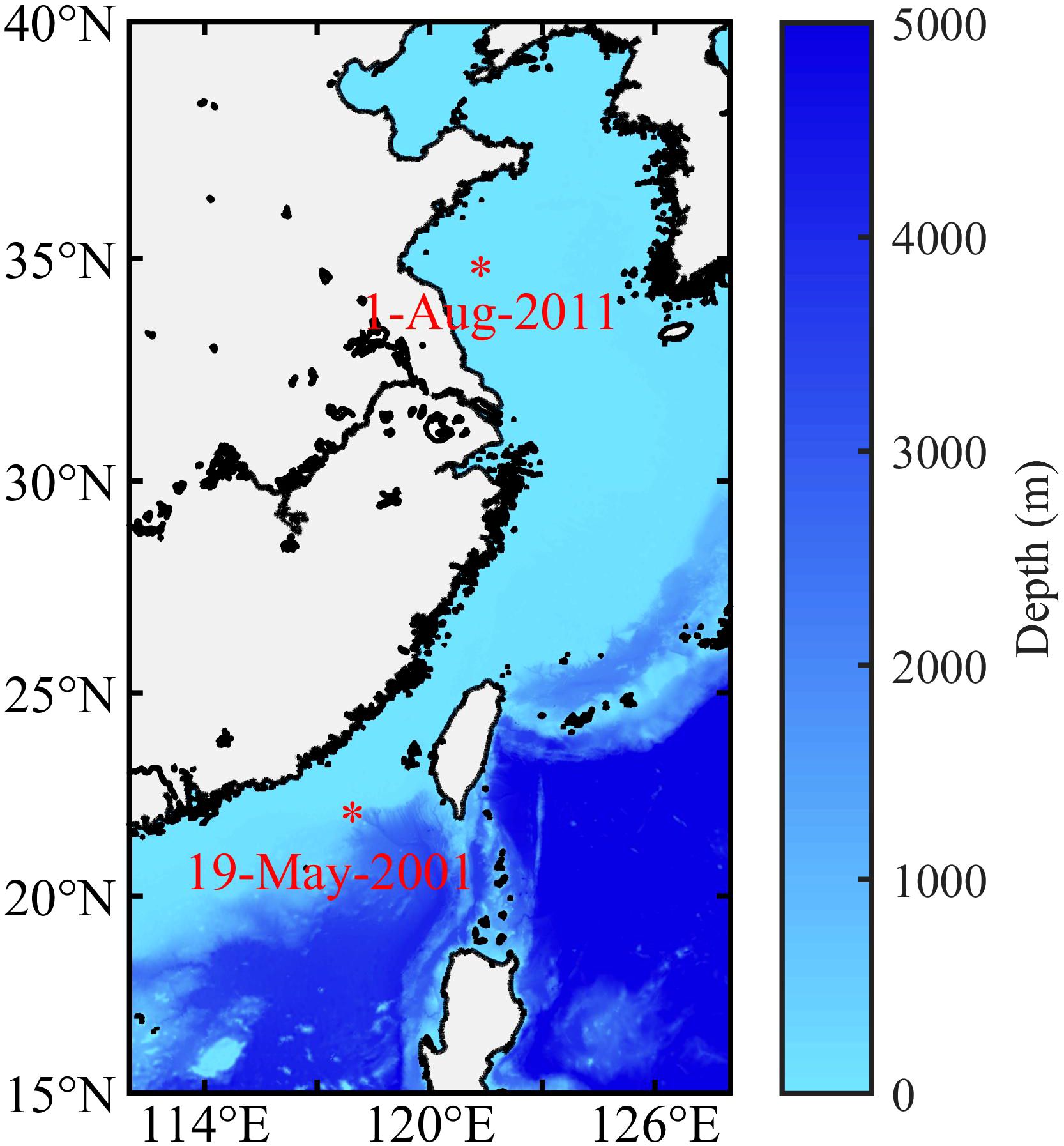
Figure 1 Locator map of the thermistor string. The asterisks show the anchor positions in the Yellow Sea and the South China Sea.

The SSP data were calculated from two sets of temperature data, collected in August 2011 in the Yellow Sea and May 2001 in the South China Sea. The SSP data for the two experiments are shown in Figure 2. In August 2011, a thermistor string was anchored offshore Tsingtao (35.66°N 121.00°E) in the Yellow Sea, where this was a semi-closed continental shelf and shallow sea. The depth was 40 m. The thermistor string was composed of 19 units, located at depths ranging from 8.9 to 31.6 m. The sampling interval was 0.5 min. In this area, cold water mass was the characteristic. Owing to intense radiation on the sea surface in the summer, the sea surface temperature rises to the annual maximum. Under the impact of these two factors, the span of mean temperature measured by the thermistor string was about 16°C, forming a strong thermocline. At the same time, The strong linear internal wave activity was noted. Under the influence of local circulation, with the measuring points located in the low-salt zone along the coast, the salinity of the water column stabilized at about 31 psu. The thermistor string, located near the continental slope (21.55°N, 117.35°E) in May 2001, was a part the measurement of the Asia Sea International Acoustic Experiment (ASIAEX). The depth was 139 m, the thermistor string was composed of 13 units ranging in depth from 21.7 to 135.1 m, and the sampling interval was 1 min. As the measuring location was in the tropics, the water temperature was higher than that in the Yellow Sea. Due to a combination of the bottom slope and transbasin waves, strong internal tidal and internal solitary wave were formed. Moreover, the variety in the amplitudes of the sound speed contour reached up to 70 m owing to internal solitary waves. The salinity was stylized at approximately 34 psu.

Figure 2

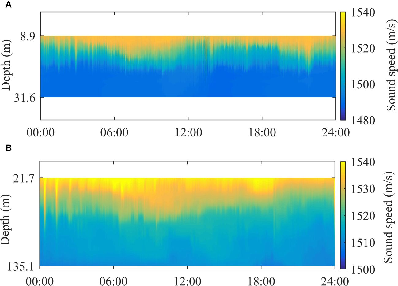
Figure 2 Variation in the SSP over 24 hours calculated from the thermistor string. (A) Yellow Sea in 2011. (B) South China Sea in 2001.

Because diurnal tidals were dominant in both areas, the cycle of a diurnal tide (24 h) was set as the time window to test using SSP models. The averaging method was applied to continuously measured in-situ data to extract the background profile. The salinity values were taken from CTD measurements near anchor positions of the thermistor string. As the variation in the salinity of multiple groups of CTD measurements was small, the salinity profile closest to the thermistor string was used. The buoyancy frequency and the ONM were calculated using the mean temperature profiles from the thermistor string and the salinity profile from the CTD. The OMB was then obtained by Equation (9). The mean temperature profiles of the thermistor did not cover the depth of the mixing layer, which might have led to extrapolation errors in the background profile under the sea surface. However, the CTD measurements in two experiments indicated that the mixing layer under the sea surface was thin, and linear extrapolation errors were thus acceptable. The OMN for mixing layers of different depths were also simulated, and the results showed that even in the presence of a thick mixing layer, the ONM values were nearly identical to those with a thin layer. Therefore, linear extrapolation was used on the depth data obtained from the thermistor string. In the subsequent analysis, the range of depth refers to the measured range of the thermistor string at a resolution of 0.1 m.

3.2 SSP reconstruction compared with EOF

The OMB and the EOF were calculated using the background profile and the SSP samples, respectively, as shown in Figure 3. The first three order on the Yellow Sea had good consistency while the first two orders for the South China Sea were similar. As the order increased, the difference between the bases increased. In general, the first three orders described a large part of the total variance. This suggests that the main statistical characteristics of SSP perturbation as determined using the EOF were consistent with the motion laws of the fluid particles determined using the OMB. Due to the impact of circulation and the geometric, dynamic activities in the South China Sea are more complex than in the Yellow Sea. This might have led to more factors contributing to the statistical perturbation component compared with that using the OMB. There were certain differences in the higher-order models, but did this not have a significant impact on the reconstruction owing to their smaller weights than in the first two orders. Some vertical perturbation features of the ONM were retained to determine the distribution of the OMB. For example, the OMB values showed an increasing number of changes in sign as the number of modes increased, and the maximum first-order amplitude appeared in the depth interval of the maximum change in sound speed.

Figure 3

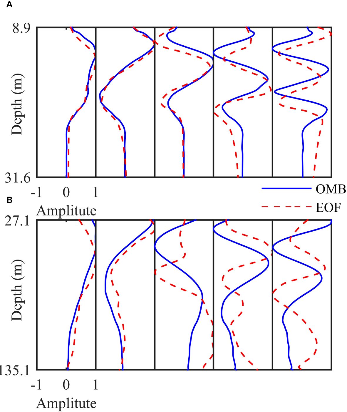
Figure 3 Comparison of the first five orders between the OMB and the EOF. (A) Yellow Sea in 2011. (B) South China Sea in 2001: from left to right are, in order, the first to the fifth orders.

Table 1 lists the cumulative proportions of variance for the different orders. It shows small differences in the proportions of the leading orders between the OMB and the EOF for each set of experimental data. The proportion of the EOF was slightly higher than that of the OMB. In case the number of samples is sufficient, the random and fine disturbances caused by some factors unrelated to the ONM can be better embodied by the EOFs. For both the EOF and the OMB, the first five orders of reconstruction exceeded 95% of the commonly used threshold, which means the resolution of the SSP reconstruction of the OMB was close to that of the EOF with a sufficient number of samples.

Table 1

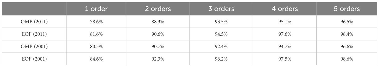
Table 1 Cumulative proportions of variance for different orders.

To analyze the reconstructions of the OMB and the EOF, the mean reconstruction error ME of a set of p discrete points and q samples is defined as follows:

$\begin{array}{ll}ME=\frac{1}{q}\sum _{j=1}^q\sqrt{\frac{1}{p}\sum _{i=1}^p(c_j(z_i)-c_j^{\prime }(z_i))},& (11)\end{array}$

where c_j (z_i) represents the SSP of the j − th sample at the i − th depth, and the apostrophe refers to the reconstruction value. The values of ME in Equation (11) of different orders are shown in Table 2. The results correspond to the results in Table 1. The EOF, with a sufficient number of samples, yielded a smaller error than the OMB. However, there was little difference in the error between them. For both seas, the OMB provided reasonable results. To illustrate the representational resolution of the OMB, the SSPs were reconstructed using the five orders of the OMB and EOF, and compared with the measured values in Figure 4. The SSP could be reconstructed accurately for the two sets of data using five orders bases. In particular for data from the South China Sea, the precision of reconstruction could still be guaranteed by the OMB even in case of significant anomalies caused by internal solitary waves. An analysis of results with large errors revealed that samples with large reconstruction errors in the two reconstruction methods were nearly identical. SSP perturbation caused by turbulence or water mass was difficult to express using the OMB, and could not constitute the principal component of perturbation (EOF). When the cumulative proportions of variance is low, their reconstruction accuracy will be affected.

Table 2

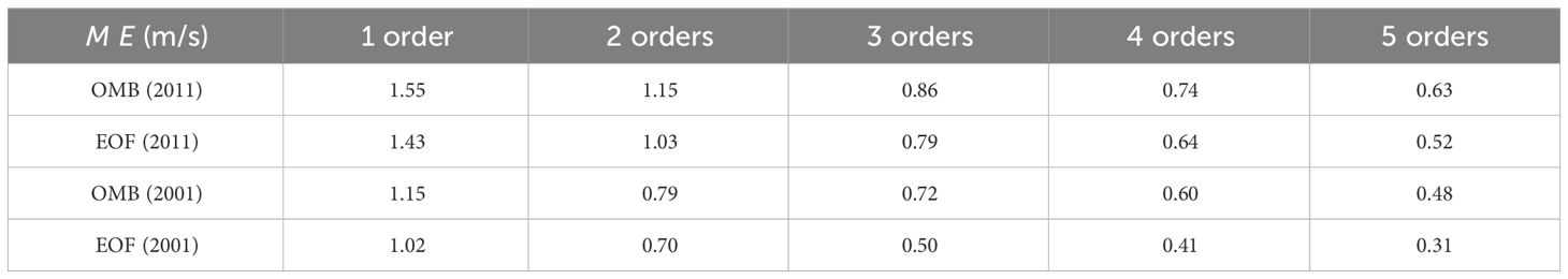
Table 2 Mean reconstruction error M E for different orders.

Figure 4

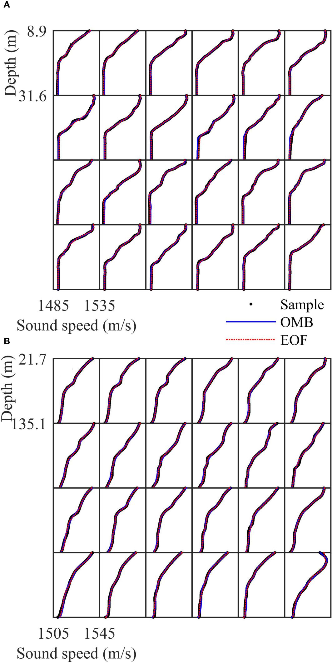
Figure 4 Comparison of SSP reconstruction of 24 example profiles on the hour from 01:00 hrs to 24:00 hrs. (A) Yellow Sea in 2011. (B) South China Sea in 2001.

3.3 Ocean dynamic analysis based on OMB

As a physical basis, the most appealing feature of the OMB is that the coefficient obtained from inversion can directly explain the ocean environment. In this section, dynamic changes in the sound speed contours (isotherm) and internal solitary waves are analyzed.

According to oceanographic analysis, different baroclinic modes correspond to different dynamic processes. The relative proportion of the ONM in an area of the sea reflects the leading dynamic activity. As it is the leading mode, it is important for the adjustment of ocean dynamics for the first two baroclinic modes. According to work by Liu (Liu, 1999; Zhang and Liu, 1999), the fluctuation resulting from Ekman pumping is mainly reflected in the first baroclinic mode, that is, changes in the depth of the thermocline. The second baroclinic mode occurs mainly due to the anomaly originating in fluctuation in buoyancy, and is manifested as a variation in the thickness of the thermocline. For the first-order ONM, the symbols were consistent in the water column, showing that the fluid particles moved in the same direction at different depths. The second-order ONM manifested as a variation in the inverse symbols of the upper and lower boundaries of the thermocline, that is, a variation in the thickness of the thermocline. Owing to the high variance of the first two orders in SSP construction, the projection coefficient of the first-order OMB can be used to represent changes in the depth of the sound speed contours in the thermocline. Furthermore, the variation in the sound speed gradient with the depth of the thermocline can be described by the projection coefficient of the second-order OMB.

Figure 5 shows a comparison of the projection coefficients and the structural parameters of the thermocline of the SSP. Figures 5A–C show that the first-order projection coefficient was in accordance with the trend of variation in the sound speed contour with depth. Figures 5B, D show similar results. The Pearson coefficients of the structural parameter of the thermocline and the corresponding projection coefficient are shown in Table 3. They suggest that the first two coefficients were highly relevant to changes in the depth of the sound speed contour and the sound speed gradient, which could be used to monitor them. The difference between reconstruction and the measured samples was small, which confirms the precision of reconstruction.

Figure 5

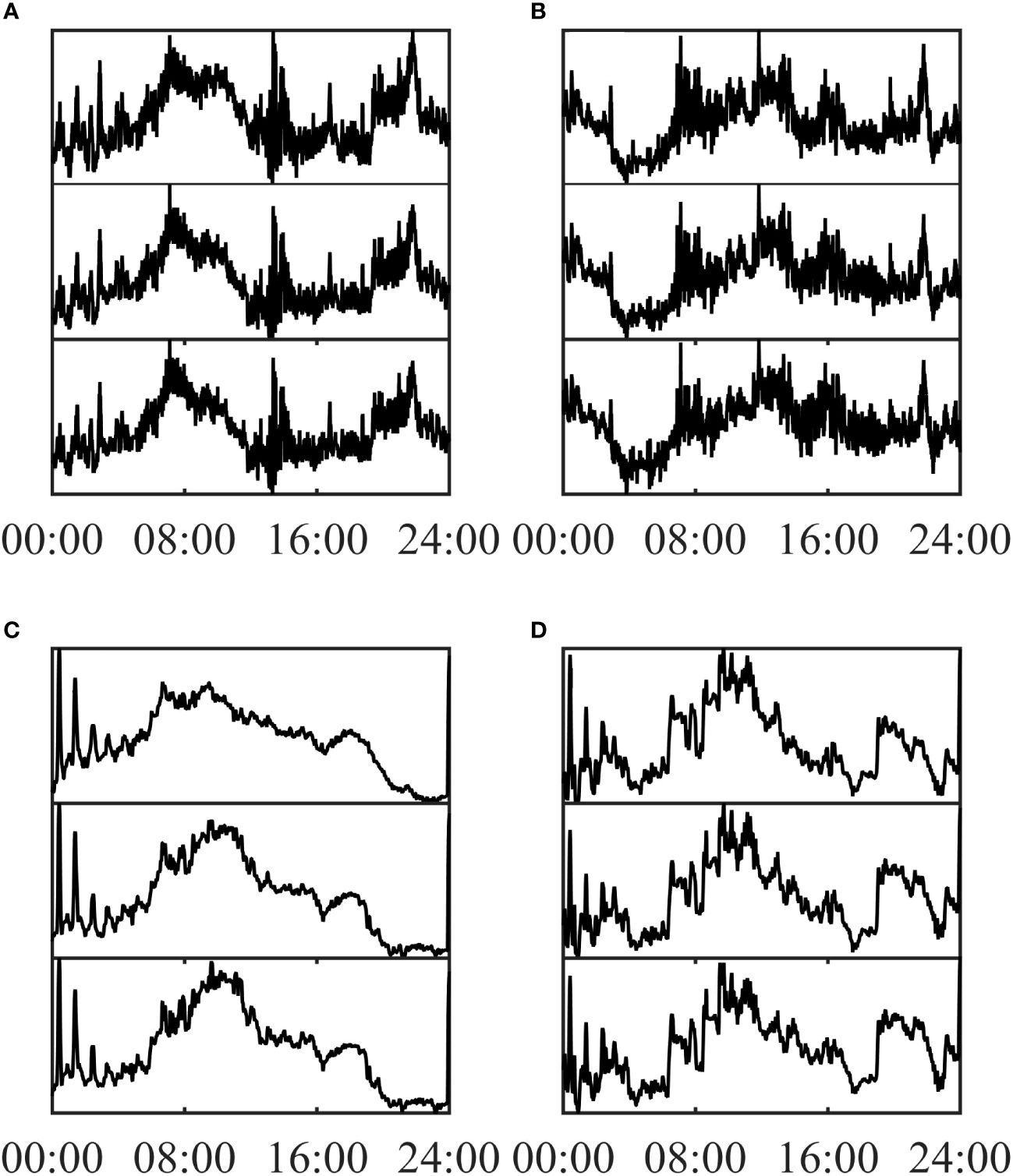
Figure 5 Comparison of the structural parameters of the thermocline and projection coefficients. (A) Depth of the sound speed contour (1518 m/s) and the first-order projection coefficient in the Yellow Sea in 2011. (B) Sound speed gradient at depths ranging from 11.4 m to 19.2 m, and the second-order projection coefficient in the Yellow Sea in 2011. (C) Depth of the sound speed contour (1528 m/s), and the first-order projection coefficient in the South China Sea in 2001. (D) Sound speed gradient at depths ranging from 24 m to 78.1 m, and the second-order projection coefficient in the South China Sea in 2001. From top to bottom, the plots show the corresponding projection coefficient, the structural parameters of the thermocline of the reconstructed SSP, and those of the sample SSP, respectively. Min–max normalization was carried out.

Table 3

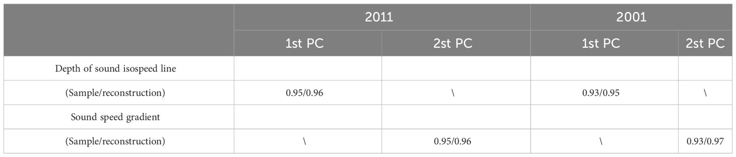
Table 3 Pearson correlation coefficient of the projection coefficient (PC) and the structural parameters of the thermocline.

The relationships among the OMBs can also help explain the dynamic activity of the ocean. $CR1=d{a}_1/dt$ is used to represent the change rate of the first-order projection coefficient, and $CR2=d{a}_2/dt$ is that in the second-order projection coefficient. According to the 2.5-dimensional internal wave Lamb model and experimental observations of the Strait of Messina, Casagrande formulated the following dynamic laws of internal solitary waves (Casagrande et al., 2009): In the first half of an internal solitary wave, the disturbance of the pycnocline at a depth is controlled by the variation of the first-order baroclinic mode, corresponding to the change in CR1. The deviation in the pycnocline can lead to opposite circulation in the upward and downward sides of its depth, where this mainly manifests as a variation in the second-order baroclinic mode, which corresponds to a change in CR2. As the first two ONMs are orthogonal, the signs of CR1 and CR2 are opposite to each other. At the end of first half of the wave, the variation in the pycnocline reaches its peaks, and the corresponding values of CR1 and CR2 are zero. In the first half of an internal solitary wave, CR1 and CR2 undergo an irregular-arch change and have opposite signs. In the second half of the wave, CR1 and CR2 undergo inverse processes to those in the first half of the wave. Thus, the variations in CR1 and CR2 are similar during an internal solitary wave. Their zero points are consistent but their signs are opposite, which indicates a double oscillation pattern.

Figure 6 shows an example of the analysis of the double oscillation pattern. The SSPs had prominent internal solitary wave trains. In the first two internal solitary waves, the CR1 and CR2 exhibited clear double oscillation patterns with a large amplitude. Although the third wave was smaller, its start and end times were identified, and it too was determined to have a double oscillation pattern. The fourth wave was visually identical but its dynamic characteristics were significantly different, and it did not have a double oscillation pattern. This analysis of the OMB confirmed waves of the internal solitary train. Furthermore, the amplitudes and wavelength characteristics could also be estimated. Double oscillation was also observed when analyzing the density EOF but not in the velocity EOF (Vázqueze et al., 2006; Casagrande et al., 2010). By contrast, the connection of the OMB to physical properties was closer. Based on the OMB and its coefficient, the dynamic activity of the ocean could be analyzed using a combination of baroclinic modes, which is useful for interpreting the results of inversion.

Figure 6

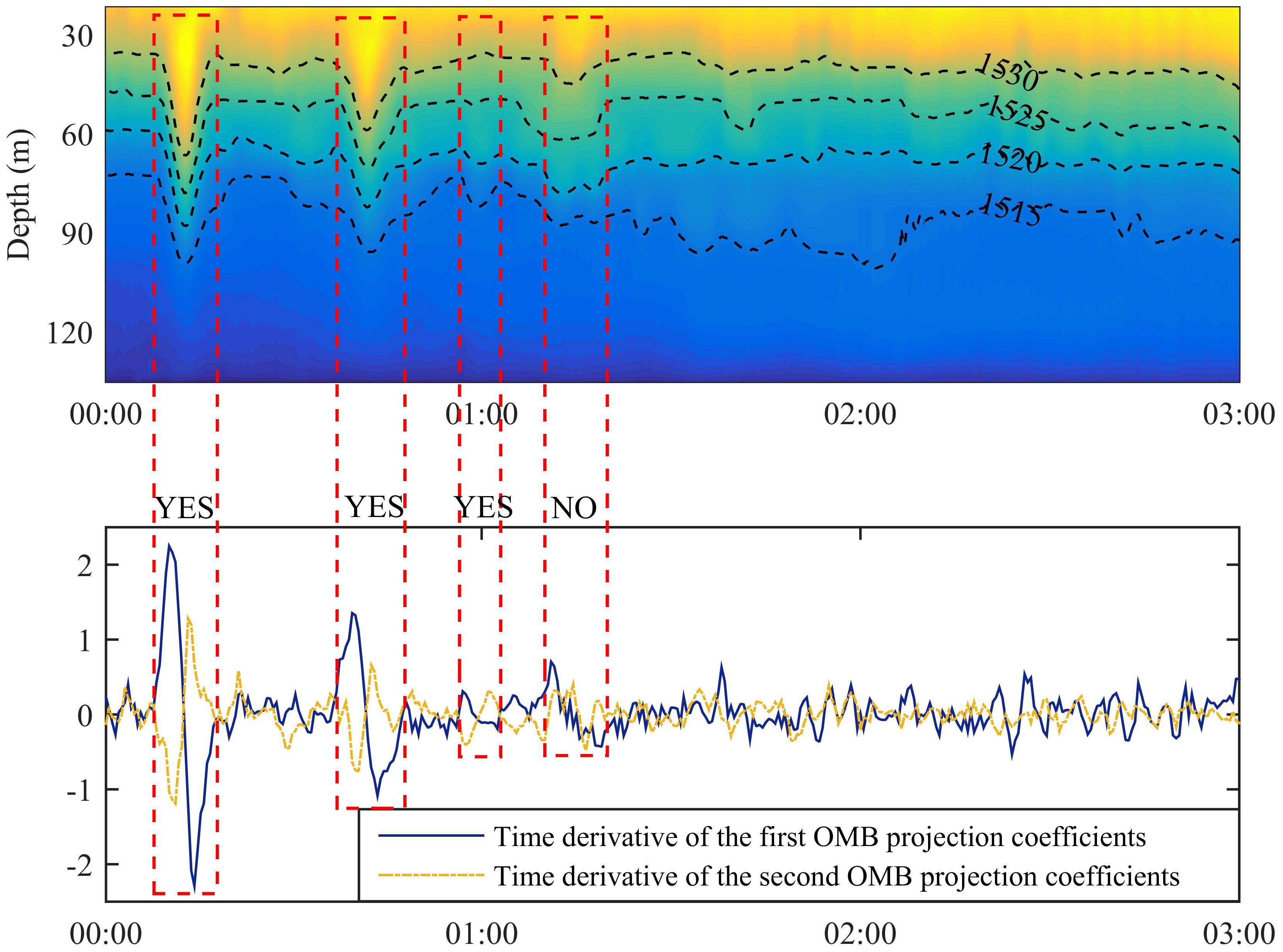
Figure 6 Internal solitary wave from 00:00 hrs to 03:00 hrs on May 19, 2001 in the South China Sea. The figure on top shows the SSPs and that at the bottom shows the corresponding CR1 and CR2. During an internal solitary wave, CR1 increased first and then returned to zero at the maximum wave amplitude. As the wave amplitude decreased, CR1 increased with the opposite sign, and then decreased to zero. The change in the amplitude of CR2 was similar to that of CR1 but opposite in sign. The patterns of changes in CR1 and CR2 are defined as double oscillation.

4 Application of OMB based on archival data

Another attractive feature of the OMB is its lax requirements of sample size. Theoretically, a representative background profile is sufficient to calculated the OMB. With the development of Argo, underwater gliders, and other measurement methods, a large number of samples of the global profile have been accumulated. In combination with ocean numerical models, many database products have been developed to provide the statistical mean and objectively analyzed mean temperature–salinity profile. In this section, the effectiveness of the OMB extracted from archival data is tested in case of the absence of in-situ data. The background profile was extracted from climatological filed data of the World Ocean Atlas 2013 (WOA13), published by the National Oceanographic Data Center (NODC, https://www.nodc.noaa.gov/OC5/woa13), and data on acoustic propagation were from ASIAEX2001 in the East China Sea.

The acoustic propagation experiment of ASIAEX2001 in the East China Sea was carried out at a depth of 105 m. A total of 32 vertical arrays were hung over a receiving ship. On the course away from the receiving ship, a launching ship released the broadband explosive sources of 38 g TNT with a rated depth of 50 m. CTD measurements were carried out many times in this experiment, and the SSPs are shown in Figure 7. Some SSPs around a depth of 60 m were low, possibly because of the cold water mass. The invariant component of the SSPs was calculated from the mean profile of all measured CTD values. As the CTD survey was not conducted during the acoustic propagation experiment, the effectiveness of the OMB was evaluated through matched field tomography, obtained by the EOF extracted from CTD samples and the OMB extracted from the archival data.

Figure 7

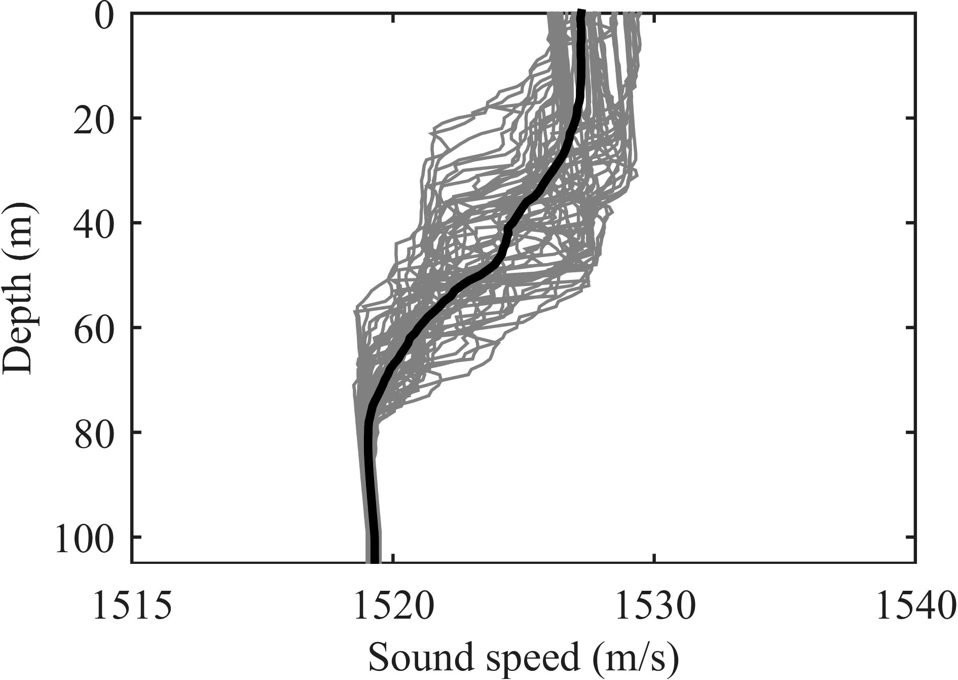
Figure 7 SSPs measured by the CTD. The dark line represents the mean SSP, and the other lines show the samples.

Considering that there were clear seasonal characteristics in the oceanic background profile, the objectively analyzed mean summer profile (1955–2012), recorded by WOA13 at a spatial resolution of 0.25°, was used. The climatological profiles of the experimental areas are shown in Figure 8. The thermocline in summer covered almost the entire water column, and salinity changed by little. At a depth of 20–70 m, the buoyant frequency was high. This corresponded to the thermocline in CTD measurements, reflecting seasonal background characteristics.

Figure 8

Figure 8 The background profiles extracted from WOA13. Buoyancy frequency was calculated based on temperature and salinity.

Based on the results of the reconstruction test, three orders with the highest reconstruction accuracy was adopted for the SSP inversion. A comparison of the first three orders of the basis between the OMB calculated by archival data and the EOF calculated by CTD samples is shown in Figure 9. A certain similarity was noted in the distribution between them, but large differences were also noted in terms of the depth of the extrema and fine structure. This indicates that the seasonal background can embody the macroscopic dynamic characteristics. However, there was a large difference between the mean climate and in-situ measurements. The key focus of the OMB application was to determine whether the resolution was sufficient to describe the SSP based on the OMB extracted from historical data products.

Figure 9

Figure 9 Comparison of the first three orders between OMB and EOF.

SSP inversion was carried out using conventional matched field processing. All environmental parameters except the projection coefficient were set as known quantities. Based on the broadband Bartlett processor, 35 frequency points in the frequency band 99–201 Hz were processed in the inversion. The optimal values of the first three orders of vector quantity a were searched using the genetic algorithm in the optimization space to implement the minimum cost function E(a):

$\begin{array}{ll}E(a)=\frac{1}{L}\sum _{l=1}^L\frac{\left|{\sum }_{n=1}^N{p}_{nl}^e(a)p_{nl}^c{(a)}^{*}\right|}{{\sum }_{n=1}^N{\left|p_{nl}^e(a)\right|}^2][{\sum }_{n=1}^N{\left|p_{nl}^c(a)\right|}^2]},& (12)\end{array}$

where L is the number of frequency points, N is the number of hydrophones, $p_{nl}^e(a)$ and $p_{nl}^c(a)$ are the measured sound pressure and the sound pressure of the replica field at the a − th frequency point, respectively, when the projection coefficient was a. The asterisk in Equation (12) indicates the conjugation. According to the experimental results, a density of 1.86 g/cm³ was set on the half space seabed. The sound speed and attenuation coefficient were 1610 m/s and 0.15 dB/λ, respectively.

Figure 10 shows the inversion results for two explosive sources 10.2 km from the receiver. It is clear that the inversion results of the OMB and the EOF were similar. The absolute errors of the two inversion results are 0.15 m/s and 0.22 m/s, respectively. The root mean square error of the two inversion results are 0.21 m/s and 0.27 m/s, respectively. This indicates that the OMB can guarantee a similar resolution to that of the EOF. In general, features of the seasonal stratification were stable, and the principal characteristics of the ocean dynamics were controlled by it. This shows that the effects of the other factors of the sea area were small. The application of the OMB without in-situ data had different effects at different times and in different spaces. In the sea area where the dynamic activities were controlled mainly by the baroclinic mode, for which reliable historical data were available, the OMB should have reasonable precision. However, in areas with complex dynamic activities, such as those influenced by air–sea interaction and water mass, and where perturbations in the sound speed are short term, in-situ measurements are indispensable to obtain an accurate background profile. Drastic perturbations at a small range of depth occurring randomly are difficult to express, whether by the physical or the statistical SSP model.

Figure 10

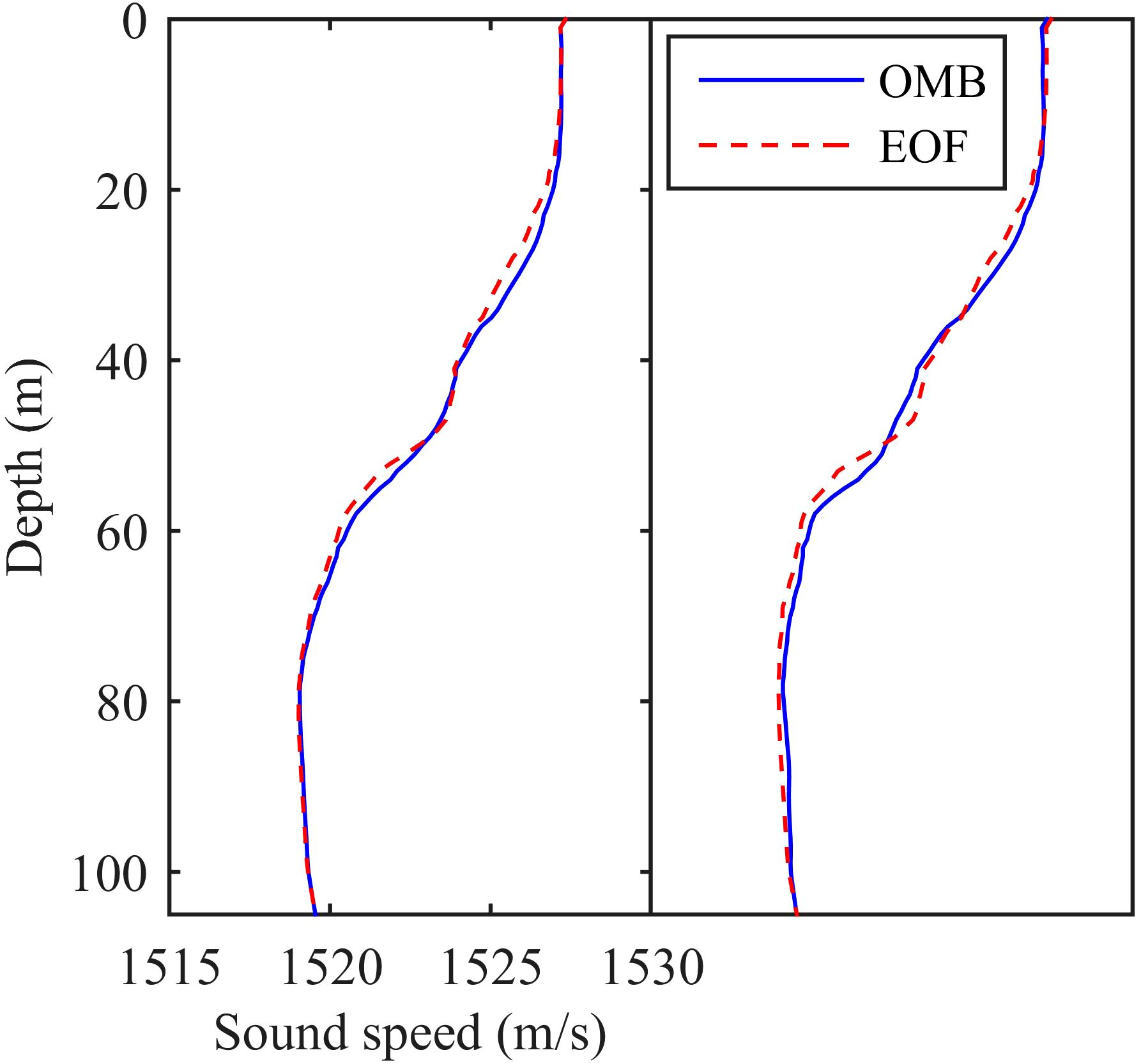
Figure 10 Two inversion results at 10.2 km. Due to the uncertainty of source depth, acoustic focalization was carried out before the SSP inversion. The actual source depth was 48 m and 49 m, respectively. The agreement between OMB and EOF is better than that in the former inversion using the rated depth of 50 m (Qu et al., 2019). Both methods have resolution to reflect the relief of source depth mismatch.

As currently available ocean data products can provide profile-related information worldwide, OMB can be theoretically calculated for applications without any in-situ measurement, where the statistical model cannot do this. However, when features of the water column stratification obtained from archival data are not consistent with the empirical situation, in-situ samples are needed for accurate SSP modeling. A compromise is to measure the profile during the slack tide to obtain stratification-related information for the OMB. This not only reduces the sample size needed, but also ensures the real-time determination of the stratification features.

5 Conclusions

The ONM is an important means of explaining the kinetic energy and heat transfer of the water column, and can be used to describe the structure of the profile. A typical example is the analysis of internal waves,

where Ursell number and Ostrovsky number calculated by ONM can effectively explain the motion and transport status of water column (Farmer et al., 2009; Yang et al., 2009). Based on this physical mode, an SSP model was proposed and tested in this paper. In contrast to the statistical model applied widely in research, the SSP perturbation described by the OMB is based on the motion law of fluid particles.

The OMB can explain the ocean environment directly through the ONM. In tests involving SSP reconstruction in the Yellow Sea and the South China Sea, the OMB yielded reasonable precision. In combination with the barotropic mode, it made possible analyses of the thermocline structures and internal solitary waves using the first two orders of the projection coefficient.

Another feature of the OMB is that it has no rigid requirement on sample size compared with the statistical model. The regional OMB was extracted through the objectively analyzed mean profile of WOA13. SSP inversion was carried out for data from ASIAEX2001 on the East China Sea, and the results of SSP inversion were similar to those of the EOF. Although the global OMB could be obtained using archival data without in-situ measurements, precision was difficult to guarantee due to the inconsistency between the mean stratification features obtained through historical data and those determined in real time. A more feasible method is to obtain the real-time background profile by few measurements. The archival data can then serve for scenarios where measurements are unavailable.

The improvement to the SSP model effected by the OMB is in providing a bridge to directly link the dynamic mechanism of the ocean with the perturbation of SSP. By using few leading orders of basis vectors and projection coefficients, it can provide a compact representation of SSPs for inversion and the determination of ocean dynamics. It presents an alternative to the statistical model.

Data availability statement

The raw data supporting the conclusions of this article will be made available by the authors, without undue reservation.

Author contributions

KQ: Conceptualization, Methodology, Writing – original draft, Writing – review & editing. WY: Project administration, Validation, Visualization, Writing – original draft. FZ: Conceptualization, Methodology, Writing – review & editing. LM: Project administration, Validation, Visualization, Writing – review & editing.

Funding

The author(s) declare financial support was received for the research, authorship, and/or publication of this article. This research was funded by the Natural Science Foundation of Guangdong Province grant number [2022A1515011519].

Conflict of interest

The authors declare that the research was conducted in the absence of any commercial or financial relationships that could be construed as a potential conflict of interest.

Publisher’s note

All claims expressed in this article are solely those of the authors and do not necessarily represent those of their affiliated organizations, or those of the publisher, the editors and the reviewers. Any product that may be evaluated in this article, or claim that may be made by its manufacturer, is not guaranteed or endorsed by the publisher.

References

Behera S. K., Rao S. K., Saji H. N. (2003). Comments on “A cautionary note on the interpretation of EOFs”. J. Clim. 16 (17), 1087–1093. doi: 10.1175/1520-0442(2003)016<1087:COACNO>2.0.CO;2

CrossRef Full Text | Google Scholar

Behringer D., Birdsall T., Brown M., Cornuelle B., Heinmiller R., Knox R., et al. (1982). A demonstration of ocean acoustic tomography. Nature 299, 121–125. doi: 10.1038/299121a0

CrossRef Full Text | Google Scholar

Bianco M., Gerstoft P. (2017). Dictionary learning of sound speed profiles. J. Acoust. Soc Am. 141, 1749–1758. doi: 10.1121/1.4977926

PubMed Abstract | CrossRef Full Text | Google Scholar

Casagrande G., Varnas A. W., Folegot T., Stephan Y. (2010). An original method for characterizing internal waves. Ocean Model. 31, 1–8. doi: 10.1016/j.ocemod.2009.07.007

CrossRef Full Text | Google Scholar

Casagrande G., Varnas A. W., Stéphan Y., Folégot T. (2009). Genesis of the coupling of internal wave modes in the strait of messina. J. Mar. Syst. 78, S191–S204. doi: 10.1016/j.jmarsys.2009.01.017

CrossRef Full Text | Google Scholar

Chen C., Ma Y., liu Y. (2018). Reconstructing sound speed profiles worldwide with sea surface data. Appl. Ocean Res. 77, 26–33. doi: 10.1016/j.apor.2018.05.002

CrossRef Full Text | Google Scholar

Cheng L., Cheng X., Zhao H., Li J., Xu W. (2022). Tensor-based basis function learning for three-dimensional sound speed fields. J. Acoust. Soc Am. 151, 269–285. doi: 10.1121/10.0009280

PubMed Abstract | CrossRef Full Text | Google Scholar

Dommenget D., Latif M. (2002). A cautionary note on the interpretation of eofs. J. Clim. 15, 261–225. doi: 10.1175/1520-0442(2002)015⟨0216:ACNOTI⟩2.0.CO;2

CrossRef Full Text | Google Scholar

Farmer D., Li Q., Park J. H. (2009). Internal wave observations in the south China sea: The role of rotation and non-linearity. Atmos.-Ocean 47, 267–280. doi: 10.3137/OC313.2009

CrossRef Full Text | Google Scholar

Gill A. E. (1982). Atmosphere-ocean dynamic (New York: Academic Press).

Google Scholar

Hjelmervik K. T., Jensen J. K., Østenstad P., Ommundsen A. (2012). Classification of acoustically stable areas using empirical orthogonal functions. Ocean Dyn. 62, 253–264. doi: 10.1007/s10236-011-0499-z

CrossRef Full Text | Google Scholar

Jiang Y., Chapman N. R. (2009). The impact of ocean sound speed variability on the uncertainty of geoacoustic parameter estimates. J. Acoust. Soc Am. 125, 2881–2895. doi: 10.1121/1.3097770

PubMed Abstract | CrossRef Full Text | Google Scholar

Kim J., Kim H., Paeng D. G., Bok T. H., Lee J. (2015). Low-salinity-induced surface sound channel in the western sea of jeju island during summe. J. Acoust. Soc Am. 137, 1576–1585. doi: 10.1121/1

PubMed Abstract | CrossRef Full Text | Google Scholar

LeBlanc L. R., Middleton F. H. (1980). An underwater acoustic sound velocity data model. J. Acoust. Soc Am. 67, 2055–2062. doi: 10.1121/1.384448

CrossRef Full Text | Google Scholar

Li Z., He L., Zhang R., Li F., Yu Y., Lin P. (2015). Sound speed profile inversion using a horizontal line array in shallow water. Sci. China Phys. Mech. Astron. 58, 014301. doi: 10.1007/s11433-014-5526-x

CrossRef Full Text | Google Scholar

Liu Z. (1999). Forced planetary wave response in a thermocline gyre. J. Phys. Oceanogr. 29, 1036–1055. doi: 10.1175/1520-0485(1999)029⟨1036:FPWRIA⟩2.0.CO;2

CrossRef Full Text | Google Scholar

Moon B. K., Yeh S. W., Dewitte B., Jhun J. G., Kirtman B. P., Kang I. S. (2004). Vertical structure variability in the equatorial pacific before and after the pacific climate shift of the 1970s. Geophys. Res. Lett. 31, L03203. doi: 10.1029/2003GL018829

CrossRef Full Text | Google Scholar

Munk W. H., Zachariasen F. (1976). Sound propagation through a fluctuating stratified ocean: Theory and observation. J. Acoust. Soc Am. 59, 818–838. doi: 10.1121/1.380933

CrossRef Full Text | Google Scholar

Qiu B., Chen S., Hacker P. (2007). Effect of mesoscale eddies on subtropical mode water variability from the kuroshio extension system study (kess). J. Phys. Oceanogr. 37, 982–1000. doi: 10.1175/JPO3097.1

CrossRef Full Text | Google Scholar

Qu K., Piao S., Zhu F. (2019). A noval method of constructing shallow water sound speed profile based on dynamic characteristic of internal tides. Acta Phys. Sin. 68, 124302. doi: 10.7498/aps.68

CrossRef Full Text | Google Scholar

Song W., Hu T., Gou S., Ma L., Lu L. (2014). A methodology to achieve the basis for the expansion of the sound speed profile. Acta Acustica 39, 11–18. doi: 10.15949/j.cnki.0371-0025.2014.01.017

CrossRef Full Text | Google Scholar

Vázqueze A., Stashchuk N., Vlasenko V., Bruno M., Izquierdo A., Gallacher P. C. (2006). Evidence of multimodal structure of the baroclinic tide in the strait of Gibraltar. Geophys. Res. Lett. 33, L17605. doi: 10.1029/2006GL026806

CrossRef Full Text | Google Scholar

Xing C., Dong S., Wan Z. (2023). Direction-of-arrival estimation based on sparse representation of fourth-order cumulants. IEEE Access 11, 128736–128744. doi: 10.1109/ACCESS.2023.3332991

CrossRef Full Text | Google Scholar

Xing C., Wu Y., Xie L., Zhang D. (2021). A sparse dictionary learning-based denoising method for underwater acoustic sensors. Appl. Acoust. 180, 108140. doi: 10.1016/j.apacoust.2021.108140

CrossRef Full Text | Google Scholar

Yang P. (2024). An imaging algorithm for high-resolution imaging sonar system. Multimed. Tools Appl. 83, 31957–31973. doi: 10.1007/s11042-023-16757-0

CrossRef Full Text | Google Scholar

Yang T. C., Liu C. H. S. H. H. J. (2017). Frequency striations induced by moving nonlinear internal waves and applications. IEEE J. Ocean. Eng. 42, 663–671. doi: 10.1109/JOE.2016.2593865

CrossRef Full Text | Google Scholar

Yang Y. J., Fang Y. C., Chang M. H., Steven S. R., Kao C. C., Tang T. Y. (2009). Observations of second baroclinic mode internal solitary waves on the continental slope of the northern south China sea. J. Geophys. Res.-Oceans. 114, C10003. doi: 10.1029/2009JC005318

CrossRef Full Text | Google Scholar

Zhang X. (2024). An efficient method for the simulation of multireceiver SAS raw signal. Multimed. Tools Appl. 83, 37351–37368. doi: 10.1007/s11042-023-16992-5

CrossRef Full Text | Google Scholar

Zhang R., Liu Z. (1999). Decadal thermocline variability in the north pacific ocean: two pathwaysaround the subtropical gyre. J. Clim. 12, 3273–3296. doi: 10.1175/1520-0442(1999)012⟨3273:DTVITN⟩2.0.CO;2

CrossRef Full Text | Google Scholar

Zhang X., Wu H., Sun H., Ying W. (2021). Multireceiver sas imagery based on monostatic conversion. IEEE J-STARS. 14, 10835–10853. doi: 10.1109/JSTARS.2021.3121405

CrossRef Full Text | Google Scholar

Zhang X., Yang P., Wang Y., Shen W., Yang J., Wang J., et al. (2024). A novel multireceiver SAS RD processor. IEEE T. Geosci. Remote 62, 4203611. doi: 10.1109/TGRS.2024.3362886

CrossRef Full Text | Google Scholar