Step change in sea surface temperatures brings marine heat waves to sub-Arctic James Bay, Canada

Marine heat waves (MHWs) are recognized as pervasive drivers of impacts on marine species and ecosystems across the world; however, sub-Arctic areas that are rapidly losing seasonal sea-ice cover remain understudied. In this research, we examine a forty-year time series of MHW characteristics in the seasonally ice-covered James Bay region of the Canadian Inland Seas in central Canada. Through the period 1982 to 2021, we document the trends and investigate past MHW occurrences with respect to their driving processes. After only two MHW events during the early portion of the record (1982-1997), five events occurred in 1998 and signaled both an anomalous year and a step change in the region’s marine climatology. The new marine climate in the region is more variable with longer and more intense MHWs. Four or more MHWs occurred in each of 2001, 2005, 2010, 2012. Events in May and October 2021 lasted over a month in duration, with the former reaching intensities of between 2.5 and 3°C. MHW intensity was correlated with ice breakup date and positive Atlantic Multi-decadal Variability, which are suggested drivers of the increasing trends in sea surface temperatures. While the impacts of MHWs on marine and coastal ecosystems in the region remain unknown because of a lack of monitoring, the 1998 MHW intensification coincides with a massive decline in the region’s seagrass Zostera marina (eelgrass) ecosystem, which has been monitored since 1982. Given projections of more extreme MHWs under global warming and the sensitivity of marine species and ecosystems to warm water events, there is an urgent need to better tracks MHWs and investigate their role in shaping northern ecosystem changes.

1 Introduction

A marine heat wave (MHW) may be defined as a coherent, long-lasting, anomalously warm event of sea surface temperature (SST) that can last from weeks to years. Their severity may be determined by the temperature anomaly, the duration of the event, or both (Frölicher and Laufkötter, 2018; Galli et al., 2017; Jacox et al., 2022). They have been observed in all major ocean basins, varying in spatial extent and water depth distribution depending on the processes that maintain them and the geometry of the region in which they occur. On smaller scales, MHWs can occur in bays, around islands, or along short sections of coastlines; however, they can also occur on larger scales in ocean basins, regional seas, or across multiple oceans (Holbrook et al., 2020). Despite increasing awareness and concern about ecological impacts of MHWs, Holbrook et al. (2019) observed that scientific understanding of MHWs is limited, especially when compared to atmospheric heat waves. In particular, the driving processes behind the high SSTs that cause MHWs are not well understood. High SST can be caused by large and small-scale oceanic forcing, atmospheric forcing, or both, and modulated by remote drivers or teleconnections (Holbrook et al., 2019; Oliver et al., 2021). The dominant mechanisms appear to be influenced by the location and season in which the MHWs occur (Frölicher and Laufkötter, 2018). However, MHW characteristics and physical drivers have been analyzed for comparatively few regions to date, limiting the potential for seasonal forecasts or management planning (Frölicher and Laufkötter, 2018; Holbrook et al., 2020; Oliver et al., 2021).

Studying past MHW events may also provide insight into their impacts on ecosystems. Based on events including El Niño events that have caused temperature stress in marine ecosystems (cf., Jarrin et al., 2022; Echavarria-Heras et al., 2006; Johnson et al., 2003) characterized in detail, it is widely accepted that under warming conditions, intense summer MHWs pose universal threats that test the established tolerance limits of ecosystems (Suursaar, 2022). Ecosystem impacts of MHWs include altered primary productivity, algal blooms, temporary or permanent shifts in habitat distribution of marine species, loss of genetic diversity and adaptive capacity, and increased human-wildlife conflict (Holbrook et al., 2020). Holbrook et al. (2020), Smith et al. (2024), and Wernberg et al. (2024) indicate that among all the ecological impacts of MHWs, effects on marine foundation species such as coral reefs, kelp forests, and seagrass meadows are particularly evident, and cumulative intensity, absolute temperature, and location within a species’ range are key factors mediating impacts.

In the Intergovernmental Panel on Climate Change’s (2019) Special Report on the Ocean and Cryosphere in a Changing Climate, the authors cite, with very high confidence, a global increase in the frequency, duration, intensity, and spatial extent of MHW events. Further, they project increased frequency of MHW events in tropical oceans and the Arctic and sub-Arctic. Sure enough, alongside increases in the global average MHW frequency and duration (Hu et al., 2020), a limited number of studies focused on the Arctic region have shown similar or more dramatic shifts in MHW duration and frequency than mid-latitude areas (Hu et al., 2020; Richaud et al., 2024). For example, Huang et al. (2021) examined MHW trends in the Arctic region from 1982 to 2020, using three SST datasets and three different MHW metrics. Comparing annual MHW metrics calculated from 1982 to 2000 and 2000 to 2020 for the Arctic Ocean, Huang et al. (2021) found that the total number of days classified as MHWs roughly doubled from 13.5 days to 28.7 days per year, while MHW frequency increased from 1.36 to 1.79 per year. The areal coverage was found to have increased from approximately 10.6% to 36.3% between 1982–2000 and 2000-2020.

With few studies having examined MHWs in Arctic and sub-Arctic waters, there is a lack of consensus on the relationship between the spatial and temporal variability of MHWs, and the relative importance of gradual ocean warming vs. other factors such as ice loss and rising air temperatures (Carvalho et al., 2021; Golubeva et al., 2021; Hu et al., 2020; Huang et al., 2021; Mohamed et al., 2022; Richaud et al., 2024). Near-surface air temperature in high-latitude areas is increasing more than three times faster than the rest of the globe (Davy and Griewank, 2023), which has been accompanied by dramatic losses in sea ice (Serreze and Meier, 2019). The increase in open water area coupled with stronger meridional heat transport has led to higher-than-average SSTs in Arctic waters, forming a positive feedback loop between sea ice loss and increasing SST (Serreze and Barry, 2011; Jenkins and Dai, 2021; Mohamed et al., 2022). However, warming and ice albedo feedback may be more or less important in some regions, for example, seasonally ice-covered northern seas vs. Arctic Ocean proper, or at certain times, reflecting the importance of abrupt transitions (cf., Ballinger et al., 2022; Carvalho et al., 2021). Because of feedbacks and abrupt changes, there is still discussion over appropriate baselines and how to define MHWs in seasonally ice-covered regions (Richaud et al., 2024). To address these sorts of gaps, Frölicher and Laufkötter (2018) pointed out the value of detailed case studies of past MHW occurrences and their driving processes. By conducting case studies in areas noted for major ecological change, there is potential to also improve our understanding of the ecological significance of these extreme events.

The Canadian Inland Seas (1.24 x 10⁶ km²), comprising Hudson Bay, Hudson Strait, Foxe Basin, and James Bay, is a marginal sea of the Arctic Ocean, downstream of Baffin Bay and the Canadian Arctic Archipelago, that brings Arctic waters into central Canada (Figure 1). The inland sea experiences an annual freeze-melt cycle, where sea ice grows from north to south from September to December, and melts between May and August; thus, the region is seasonally ice covered (Hochheim and Barber, 2014; Andrews et al., 2018). A feedback loop exists between sea ice and SST, whereby the timing of ice breakup/melt influences the amount of heat stored in surface waters in summer, which then affects the timing of ice freeze-up (Andrews et al., 2018; Crawford et al., 2023).

Figure 1

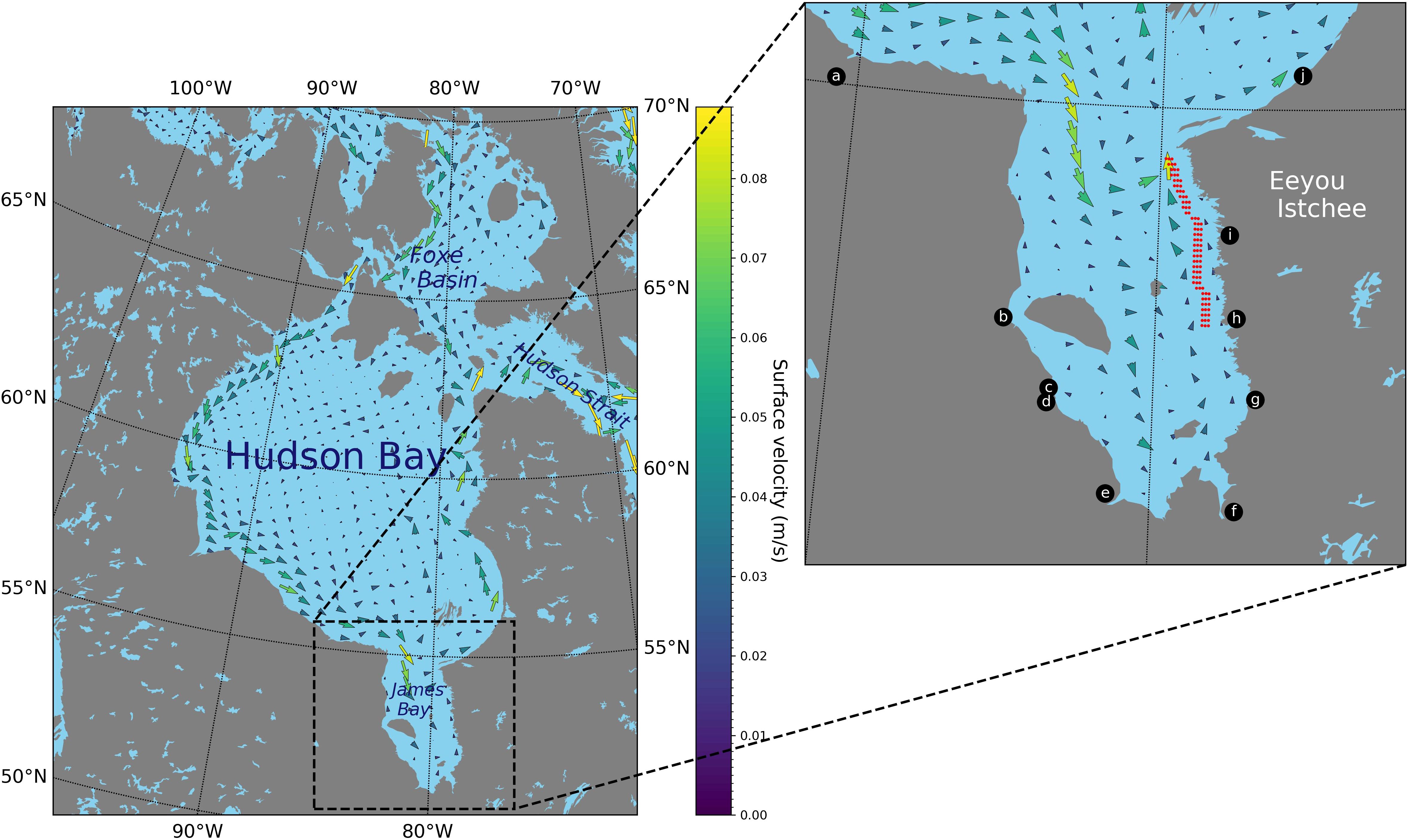
Figure 1. James Bay within the Canadian Inland Seas in central Canada. The points used to obtain daily mean SSTs are highlighted in red. Nearby communities are labeled as follows: (a) Peawanuck, (b) Attawapiskat, (c) Kashechewan, (d) Fort Albany, (e) Moosonee, (f) Waskaganish, (g) Eastmain, (h) Wemindji, (i) Chisasibi, (j) Kuujjuarapik. Surface currents are calculated from the ORAS5 zonal and meridional velocity components averaged over 1982 to 2021 (C3S CDS, 2021).

James Bay is a shallow bay of ~68,000 km² extending southward from Hudson Bay. It may be expected to be vulnerable to increasing MHW events related to rapidly rising air temperatures and loss of sea ice because of its low latitude, continental setting, and >4 m annual freshwater addition from river runoff and sea-ice melt. However, research in the bay remains limited and has so far not been able to address coastal communities’ questions about the causes of change in the ice and ocean systems (cf., McDonald et al., 1997; Cree Nation of Chisasibi, 2015). The coverage of landfast ice in James Bay has already been impacted in certain areas along the coast and further recession and delayed freeze-up is projected by the year 2050 (Taha et al., 2019), with implications for polar bears and other ice-associated wildlife (Stroeve et al., 2024). Changes in the ice regime of James Bay have the potential to impact SSTs and shift trends in the frequency, duration, and extent of MHWs, thus widely impacting sensitive ecosystems in the region.

The Arctic and sub-Arctic marine and coastal environments are changing at a very rapid pace. Evidence from marine mammal and bird monitoring programs and observations of Indigenous Peoples suggests that profound ecosystem changes have occurred in these regions during recent decades (cf., Ferguson et al., 2010; Worden et al., 2020). With MHWs adding a further challenge to northern coastal ecosystems that are already responding to warming trends, watershed and hydrologic changes (cf., Stadnyk et al., 2021), and a shorter season of sea-ice cover and associated biogeochemical changes (cf., Lannuzel et al., 2020), there is an urgent need to improve understanding of the causes and consequences of MHWs and to incorporate MHW tracking into ecosystem monitoring efforts.

2 Objectives

Here, we undertake three objectives. First, we examine the characteristics of MHWs in eastern James Bay through the period 1982 to 2021, which corresponds to the period of monitoring of the region’s seagrass, Zostera marina, (eelgrass) ecosystem (Leblanc et al., 2023). This sub-Arctic eelgrass ecosystem, once considered among the largest in North America (Lalumière et al., 1994), has shown limited recovery following a massive decline in the late 1990s (Leblanc et al., 2023; Davis et al., 2024; Idrobo et al., 2024). Second, we study air temperatures, ice cover, and large-scale atmospheric patterns to investigate their role in shaping the MHW characteristics and trends over this 40-year period. We focus our analysis on eastern James Bay along the coast of Eeyou Istchee, and the open-water growing season (May – October).

We use the MHW definition by Hobday et al. (2016), which does not assume any specific driver (atmospheric or oceanic) or that a MHW has any particular impact. It allows the MHW to be defined relative to a baseline climatology for comparison of intensity, duration, and spatial extent at a given time of year, which means MHWs can be studied year-round and not exclusively in warmer months (Hobday et al., 2016). By improving our understanding of past and present MHWs in James Bay, as well as their temporal trend, their role in ecological changes in the region may be better assessed.

Our third objective is to examine the influence of using different baseline periods in the MHW analysis. The identification of an appropriate baseline for detecting and characterizing MHWs is recognized as a particular challenge for seasonally ice-covered Arctic and sub-Arctic areas (cf., discussion in Oliver et al., 2021; Richaud et al., 2024). Some workers have found that detected MHWs are longer and more intense when using a longer baseline of 30 years or more (Richaud et al., 2024), whereas others have found that the length of the baseline makes no significant difference but presence of long-term trends in a time series has large effects (cf., Schlegel et al., 2019).

3 Data and methods

3.1 Study area

James Bay (outlined in Figure 1) has a surface area of approximately 68,000 km². It is relatively shallow, with depths greater than 50 m in only a few places (Prinsenberg, 1986a). It is supplied by seawater from Hudson Bay, which in turn receives outflow from the Arctic Ocean via Fury and Hecla Strait/Foxe Channel and Baffin Bay/Hudson Strait. According to Prinsenberg (1986a), James Bay exhibits on average a cyclonic surface circulation and an estuarine-like twolayer circulation with inflow of saline water in deeper layers and outflow of river diluted water in the surface layer. Cold and relatively high saline water that enters the bay is heated and diluted as it flows cyclonically around James Bay, and then leaves on the surface as it flows northward primarily along the eastern shore (Prinsenberg, 1986a; Ridenour et al., 2019).

The hydrography of the Canadian Inland Seas depends on seasonal cycles of freshwater input, the sea-air heat flux, and ice cover (Prinsenberg, 1986b). The mean runoff rate per unit drainage area within the system increases from north to south, reaching a maximum in James Bay. Seasonal cycles of runoff rates in James Bay are characterized by low values in the winter and high values in the spring, called freshets. The spring freshet occurs in May and early June in James Bay, and strongly influences the timing and breakup of the ice cover (Prinsenberg, 1986b).

The ice regime in James Bay begins with freeze-up in early December, and the initial formation of ice occurs in coves and river estuaries over freshwater (Taha et al., 2019). Landfast ice forms along the margins of James Bay, however, offshore pack ice remains mobile throughout the winter due to strong tides and wind (Gupta et al., 2022). Ice breakup occurs unevenly and variably across the James Bay during May to June in the spring through the action of wind and currents under warm conditions, though it is uncertain which of these conditions (air temperature, warm freshwater, or solar radiation) is predominant (Taha et al., 2019; Gupta et al., 2022). Ice may drift in from southern Hudson Bay and/or linger around northwest James Bay, but typically James Bay is completely ice free by the end of July. There have been numerous changes in regional hydrology resulting from both climate change and hydroelectric development (Stadnyk et al., 2021; Ingram and Larouche, 1987; Messier et al., 1989; Peck et al., 2022; de Melo et al., 2022). Eastern James Bay receives freshwater inflows from thirty-eight watersheds that drain a total area of approximately 386,880 km² in northern Quebec, Canada. The La Grande River is by far the largest river with a watershed area of approximately 210,000 km², and annual average discharge of 3782 m³ s^-1 following various river diversions (de Melo et al., 2022). This is the first study to assess severity and trends in extreme climate events.

3.2 Sea surface temperature dataset

Because of potential biases in satellite derived SST data sets for seasonally/partially ice-covered areas (cf., Richaud et al., 2024), we carefully selected the Operational Sea Surface Temperature and Sea Ice Analysis (OSTIA) data set for this work after considering all the alternatives. The OSTIA system generates high-resolution (1/20° grid), daily, global, gap-filled SST fields derived from satellite and in situ data. It has a minimum SST value of -1.8°C, which is typically associated with sea ice concentration exceeding 90%. Described in Donlon et al. (2012), OSTIA was initially developed by the UK Met Office in response to a growing need for a timely, accurate, high-resolution SST product for Numerical Weather Prediction and Numerical Ocean Forecasting, new coupled ocean-atmosphere systems, and for developing high-resolution climatological records of SST (UK Met Office, 2012). The SST and sea ice data sources used to create OSTIA include various satellite infrared and passive microwave sensors and in situ data from ships and moored and drifting buoys (Donlon et al., 2012). This system has been continuously developed since its first release, including the selection of input data, as new satellite sensors are added if they improve data quality and removed if they fail or the quality of their data degrades (Good et al., 2020). In this work, we use OSTIA to analyze the late spring, summer, and fall periods (May through October; henceforth called the ‘study period’) for each year from 1982 to 2021, creating a 40-year reference period. For the SST time series analysis and defining MHW events, the data are subset to the gridpoints in northeastern James Bay shown in Figure 1.

Other studies on MHWs in the Arctic region have used the Daily Optimum Interpolation Sea Surface Temperature dataset from the National Oceanic and Atmospheric Administration (NOAA) (e.g., Thoral et al., 2022; Huang et al., 2021; Hu et al., 2020). However, their work covered very large geographic areas (at minimum, the entirety of the Arctic Ocean). As our work focuses on the eelgrass-dominated region in eastern James Bay (Figure 1, inset), we opt to use a high-resolution SST dataset. Huang et al. (2023) assessed the performance of OSTIA and eight other gridded SST datasets. Huang et al. (2023) note that the quality of a gridded SST product is typically assessed by comparison to a reference SST; in situ SSTs from buoys are considered an ideal reference due to their high accuracy and high spatial and temporal coverage. After averaging the reference SSTs onto a common 0.25° × 0.25° grid, the magnitude of root-mean square differences in OSTIA relative to point (buoy) observations was found to be the second lowest of the nine SST datasets. On its original grid, standard deviations were smallest in OSTIA, which suggests an advantage of high-resolution analyses for resolving finer-scale SSTs (Huang et al., 2023).

We determined the ice break-up and freeze-up dates from the sea ice concentration data contained in each daily OSTIA SST file. We use the latest date in each year with less than 50% sea ice concentration and the earliest date with greater than 50% sea ice concentration, respectively. In the SST analysis, SSTs under ice with concentration greater than 50% are relaxed toward 271.35 K, with a timescale varying between ~17.5 days to ~5 days linearly with ice concentration from 50% to 100% (Good et al., 2020).

3.3 SST analysis and MHW definition

Similar to Hobday et al. (2016), MHWs are defined relative to a baseline temperature climatology and relative to a high percentile threshold. In this research, we use the 40-year SST climatology of the OSTIA dataset and the 90th percentile threshold. A five-day moving average is applied to the 90th percentile calculation. Next, a MHW event is defined as a period of five days or more for which the original SST (with no moving average) exceeds the 90th percentile; further, when there are gaps between events of two days or less, these events are considered continuous (Hobday et al., 2016). Both the spatial and temporal aspects of MHWs are considered, using indices that consider variables like maximum value, duration, and magnitude relative to climatological norms (Suursaar, 2022). Note that in section 5.1, we examine the effects of using different baselines other than the 40-year SST climatology for MHW detection.

To describe temporal variability of MHWs in James Bay during the open water season from 1982 to 2021, we examine parameters of frequency, duration, and intensity, using the daily mean SST of the points outlined in Figure 1. Frequency is defined as the number of discrete events lasting five days or longer. The duration of an event is defined as the number of days the mean daily SST remained above the 90th percentile of the 40-year climatology for a given day. The intensity of an event is defined as the number of degrees above the 90th percentile, represented by the scale in Figure 2.

Figure 2

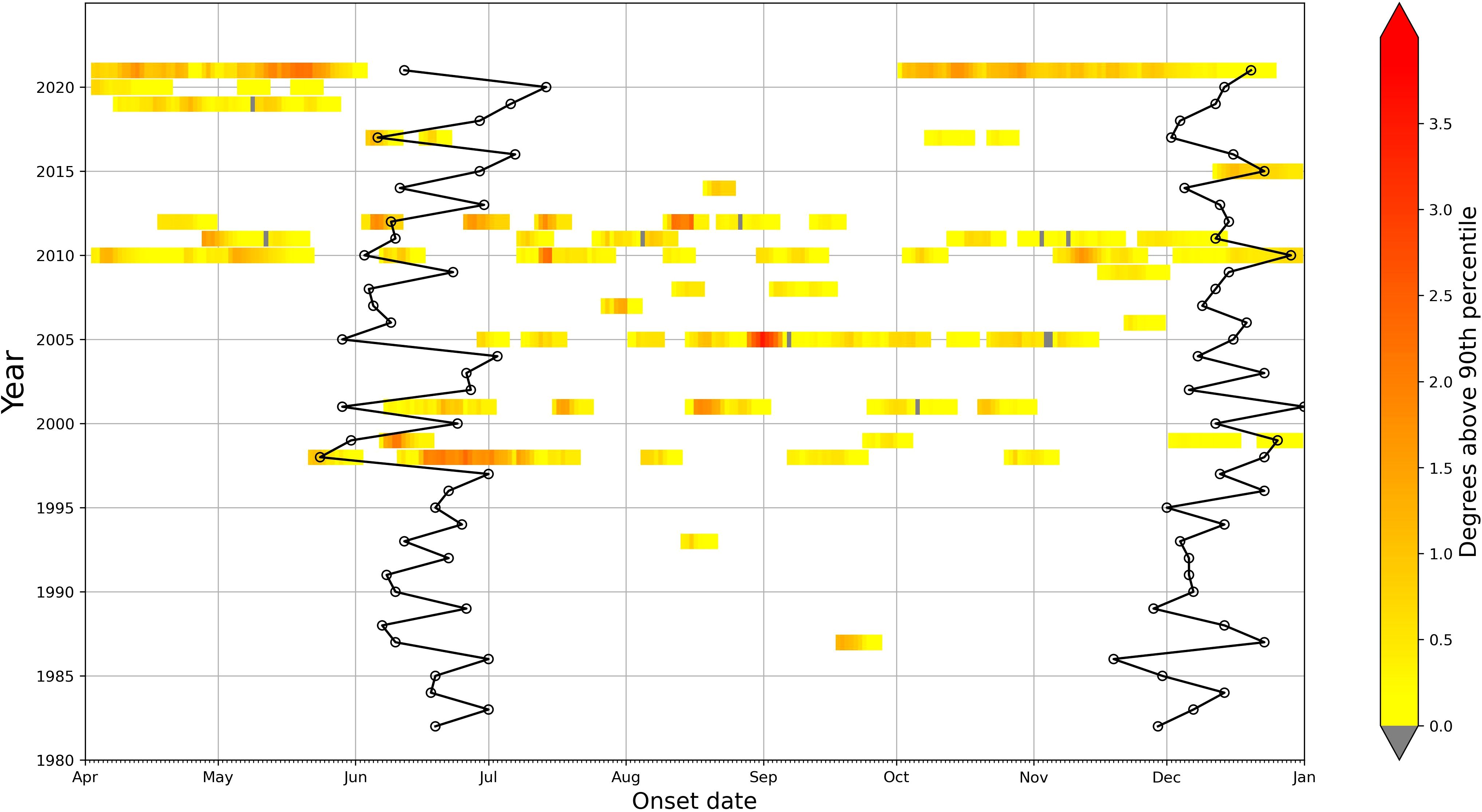
Figure 2. Plot of MHW frequency, duration, and intensity for 1982 to 2021 for eastern James Bay using SST data from the OSTIA dataset. The black lines represent the ice breakup and freeze-up dates based on a threshold of 50% sea ice concentration in the OSTIA dataset. Grey indicates periods of two days or less that connect two MHW events.

We also examine monthly average SST for each month in the study period. We use Pettitt change-point analysis to indicate shifts in central tendency and subsequently significant shifts in temporal dynamics, and the non-parametric Theil-Sen (or Sen’s slope) estimator to estimate the direction and intensity of trends before and after these shifts, as it is considered more robust to outliers than standard linear regression (Thoral et al., 2022). We further use the non-parametric rank-based Mann-Kendall test to determine if there were trends and Spearman’s rho to test for correlation between independent datasets. To investigate mechanisms leading to MHWs in James Bay, we used Spearman’s rho to test for correlation between monthly SSTs and ice break-up date, ERA5 2-m air temperature (Hersbach et al., 2023), and the Atlantic Multidecadal Variability (AMV) index (Huang et al., 2017). This was done for each month in the study period and for before and after the change-point year, determined using the Pettitt test.

4 Results

4.1 MHW frequency, duration, and intensity over 1982-2021

From 1982 to 2021, 50 sustained high SST events occurred within (or at least partially within) the May-October study period in eastern James Bay that meet the MHW definition outlined by Hobday et al. (2016) (Figure 2). The first two MHW events on the satellite record occurred in September 1987 and August 1993, and persisted for 8 and 6 days, respectively. The number of MHW events increased to five in 1998. The first of these was in May 1998, when the area would have still been ice-covered during an average year. The second started on 11 June 1998 and was extreme within the 1982–2021 record in both its duration (41 days) and intensity for the time of year. No similar June MHW event has occurred since, despite warming conditions and reduced ice coverage.

In contrast to the weak and infrequent MHW events before 1998, many events (43) occurred after that calendar year, and many achieved moderate- to high intensity (>2°C; see orange-red shading in Figure 2). The events were clustered, producing several intense MHW seasons or, in some cases, several intense MHW years. For example, after the intense MHW season in 1998, which had a total of 78 days of MHWs, there were also three or more MHW events occurring in each of 1999 and 2001, for a total of 19 and 75 days, respectively (Figure 3; Supplementary Table S1). In 2005, the most intense event of the entire 40-year record occurred, with an intensity exceeding 3.5°C in late August – early September. This event also had a long duration, beginning in August and ending in early October. In total, there were 86 days of MHWs in 2005. After this intense season, during 2006-2009, MHWs occurred only in 2007 (one event lasting 7 days) and 2008 (two events lasting in total 18 days) and these events had relatively low intensity.

Figure 3

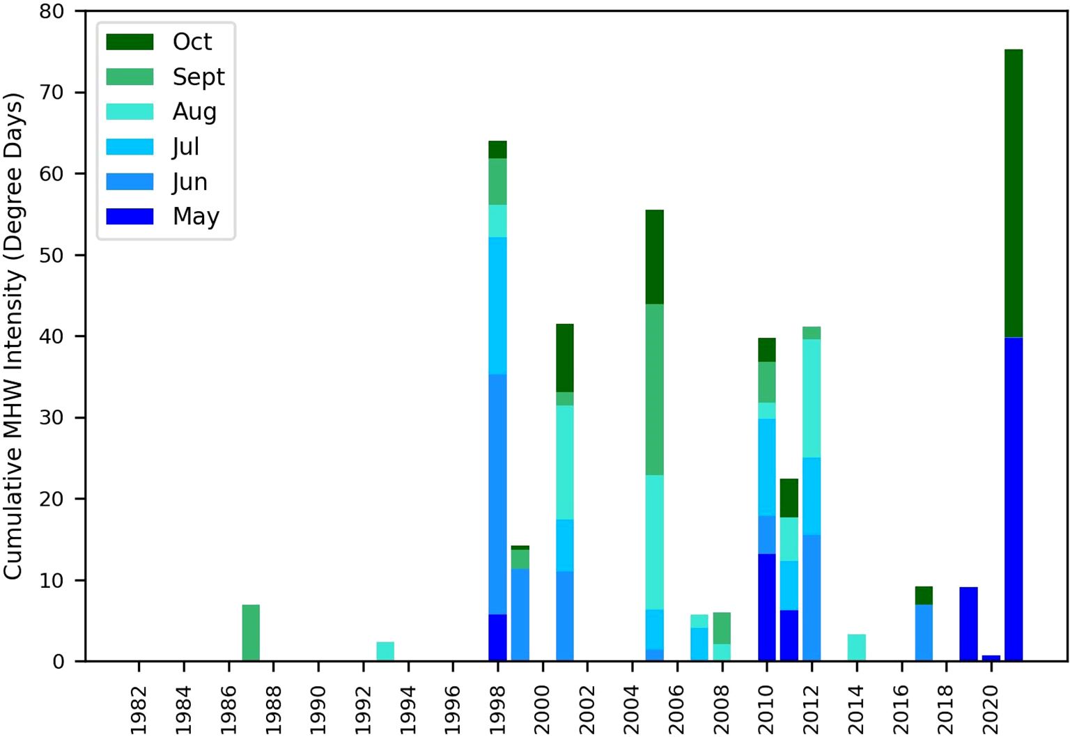
Figure 3. Monthly and annual cumulative marine heat wave intensity (degree days relative to the 90th percentile).

From 2010 to 2012, there was again a high frequency of MHWs, with at least five events occurring in each of 2010, 2011, and 2012. There were, in total, 75, 54, and 46 days of MHWs in 2010, 2011, and 2012 during the May-October study period but note that some events occurred only partially within the May-October study period and extended into November. After 2012, there was one short, low-intensity event, less than 1.5°C above the 90^th percentile, in August 2014, followed by no events in 2015 or 2016. The next intense period of MHWs started in 2017. MHWs occurred in four of the following five years (2017, 2019, 2020, and 2021). There were as many as four events during each of these years and, in total, 25, 25, 10, and 62 days of MHWs. The MHW events in 2021 (one peaking in May and another peaking in October) are notable as they each lasted over a month in duration, with the first reaching intensities between 2.5°C and 3.0°C and the second peaking at between 1.5°C and 2.0°C.

In addition to increasing frequency and intensity of MHWs over time, a second notable shift is in the seasonal distribution of the events. In 1998, the MHW season started exceptionally early in May and June, months during which there had not been any MHW events previously. In 2010, MHWs began occurring both earlier and later in the study period and even in the months outside the normal open-water period such as April and December. There had been only one December MHW event in the record prior to 2010, which took place in 1999, but December events occurred not uncommonly after 2010 (Figure 2). Further, while MHW events occurred throughout the May-October study period in 2010, 2011, and 2012, they occurred exclusively in May, June, and October in 2017, 2019, 2020, and 2021. During those years, there were no MHW events during the normal warm months of July, August, and September.

4.2 Cumulative MHWs intensity

To obtain a measure that integrates MHW duration and intensity, we calculated cumulative intensity of the MHWs for each month and in each year. Several studies (e.g., Chauhan et al., 2023; Zhang et al., 2022) have used cumulative intensity to characterize MHWs over a reference period and it has been argued that indices based on cumulative values rather than temporal averages are preferable because assessing intensity through averaged values does not allow for unequivocal comparison of event magnitude when they differ in length (Russo and Domeisen, 2023). As shown in Figure 3, the cumulative MHW intensity increases throughout the reference period, with a notable jump in 1998 to 63.9°C day from previous maxima of 6.9°C day and 2.3°C day in 1987 and 1993, respectively. The highest recorded cumulative intensity of MHWs was 75.3°C day in 2021 (Figure 3). For statistical analysis, we describe the change in cumulative intensity over the 40-year reference period using Spearman’s rho test and separating out two ‘seasonal’ cumulative intensities: May, June, and July (MJJ) and August, September, and October (ASO). For MJJ, the increase in seasonal cumulative MHW intensity was statistically significant over 1982-2021 (ρ = 0.466, p = 0.002). For ASO, there was a marginal relationship (ρ = 0.295, p = 0.06). Thus, we can conclude unequivocally that spring-early summer MHWs have intensified in James Bay over 1982-2021.

We also examined the correlation between ice breakup date and the seasonal cumulative MHW intensities. As expected, the correlation between ice breakup and MJJ cumulative intensity was negative and statistically significant (ρ = -0.463, p = 0.002). Surprisingly, the correlation between ASO cumulative intensity and ice breakup date was also significant and even stronger with ρ = -0.737 and p < 0.0001. These correlations suggest an increase in MHW intensity with earlier ice breakup and show that early ice breakup date increases MHW intensity throughout the open-water period.

4.3 Monthly climatology for SST over 1982-2021

Using the SST data from which the MHW events were identified, the climatology for SST for each month of the study period (May through October) was examined using the Theil-Sen and Pettitt tests. The Pettitt change-point analysis yielded statistically significant change-point years at the 95% confidence interval for each month in the study period (Figure 4). These change-points represent a break in the 40-year time series that divides the series into two time periods, whereby the change-point year is the last year of the first time period. Thus, the change-point year for May, June, and July was 1997, which means the shift in the SST trend occurred in 1998. The change-point years in August, September, and October were 1994, 1995, and 1996, respectively (Figure 4).

Figure 4

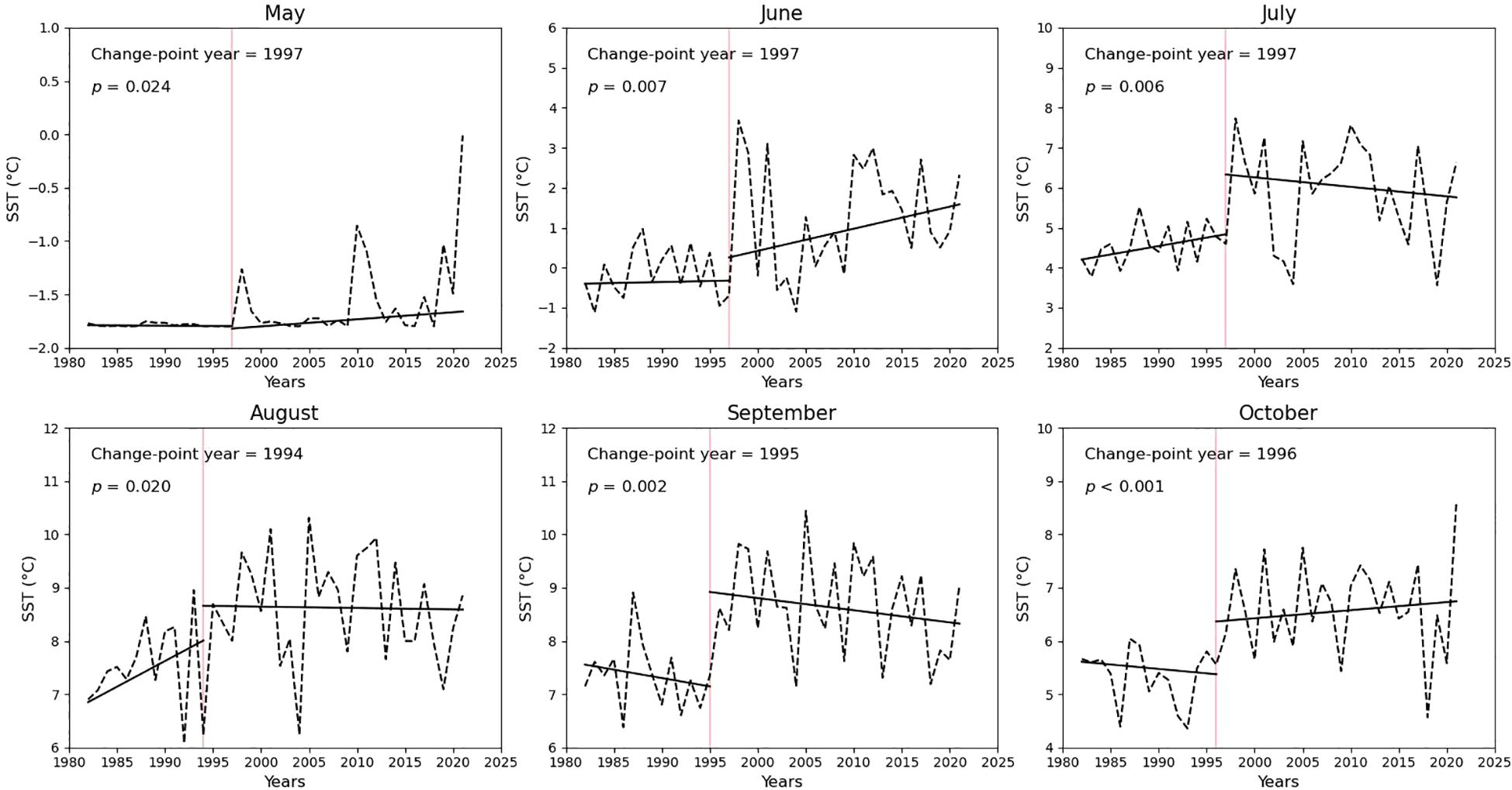
Figure 4. Theil-Sen regression and Pettitt change-point analysis of monthly SST for the study period for 1982 to 2021. The change-point years and p values from the Pettitt test are reported for each month. The red line is a visual representation of the change-point year.

The Theil-Sen test was used to test the regression slopes before and after the change-point years for each month in the study period (Figure 4). Prior to the change-point year, May, September, and October had negative slopes (i.e., decreasing trends) of SST while June, July, and August had positive slopes (i.e., increasing trends). After the change-point years, May, June, and October had positive slopes and July, August, and September had negative slopes (Figure 4). However, based on Mann-Kendall trend tests (Mann-Kendall; Hussain and Mahmud, 2019), none of these trends were statistically significant at the 95% confidence interval.

4.4 Statistical associations between SST and other variables

The increase in SSTs after the shift in the late 1990s coincides with a shift toward more variable and often earlier ice break-up dates (Figure 5). Fully 32% of the break-up dates after 1997 are earlier than the earliest break-up date 1982-1997, and 16% of the break-up dates after 1997 are later than the latest break-up date 1982-1997. Additionally, visual comparison of the MHW time series and ice break-up dates (represented by the black circles and lines in May, June, and July in Figure 2) suggests a possible association between early ice break-up and MHW occurrence during the open water period of that calendar year, which was confirmed by significant negative correlations between monthly SSTs and ice breakup day-of-year (DOY) (Table 1). Monthly average SST increased as the DOY decreased (Figure 5); in other words, higher SSTs were associated with ice breakup occurring earlier in the year. The associations between SST and ice breakup date were strong for several months including June, July, and August, and were present in the data set both before and after the change point years, although, in some cases, specific trends changed (Table 1). For example, June SSTs were strongly associated with ice breakup date before 1997 (ρ = -0.858) and less strongly associated after 1997 (ρ = -0.627). Ice freeze-up date was positively associated with SST but the associations were quite weak across all months (maximum ρ = +0.567 for September during the later part of the study period after 1996).

Figure 5

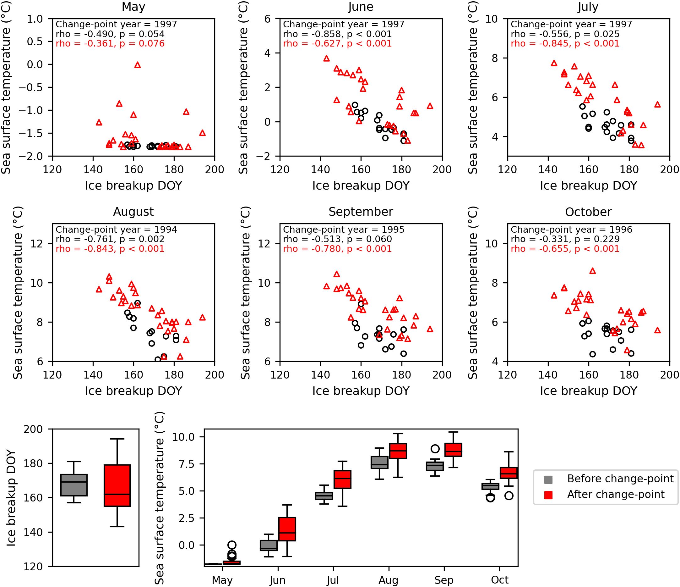
Figure 5. Correlation between monthly average OSTIA SST and ice break-up date for 1982 to 2021. Black circles represent the data up to and including the change-point year while red triangles represent the data after the change-point year. Bottom row shows the distribution of ice break-up date and monthly SST before (gray) and after (red) the change-point year. Boxes indicate the interquartile range, whiskers extend up to 1.5 times the interquartile range, circles indicate outliers, and the horizontal line is the mean.

Table 1

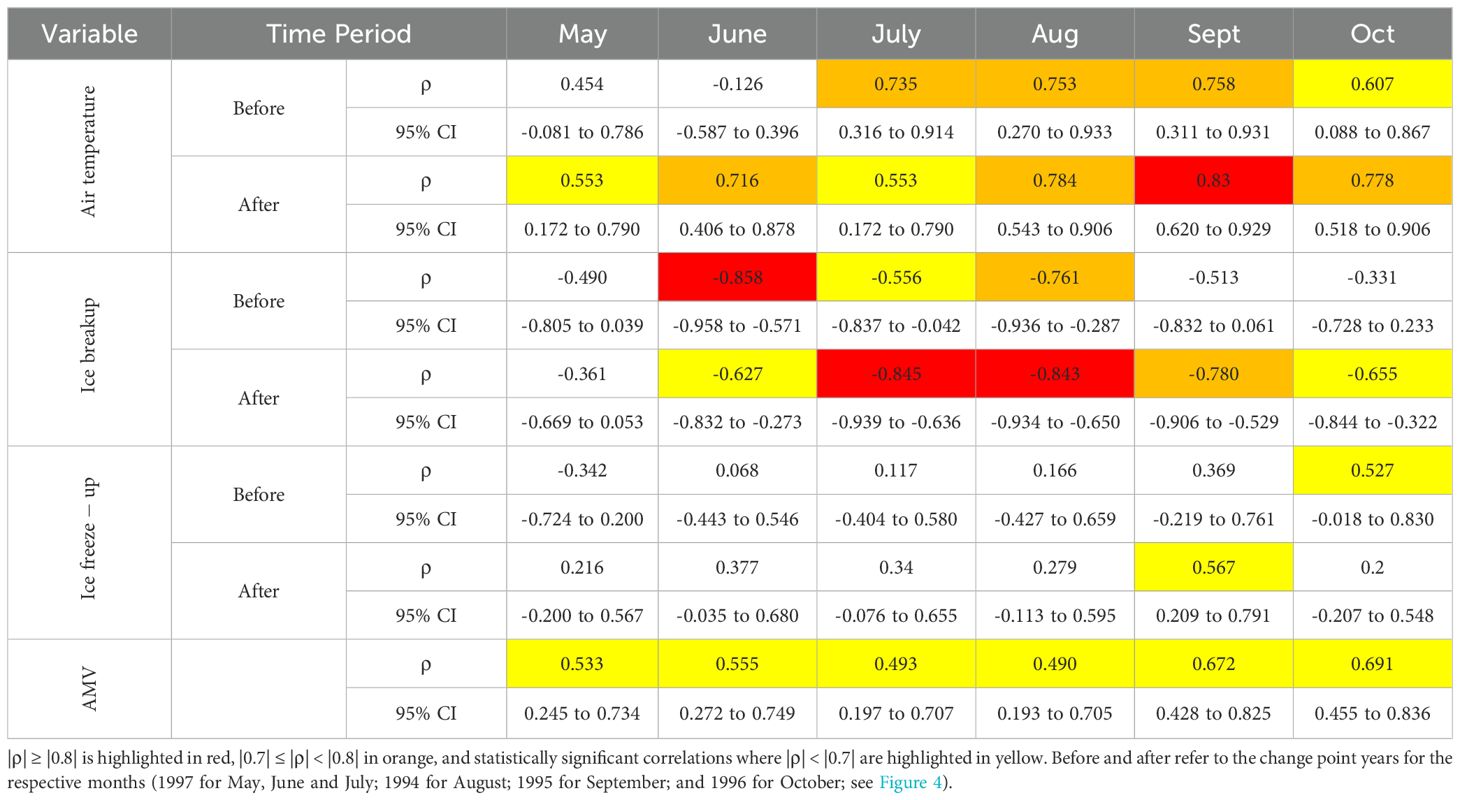
Table 1. Summary table of Spearman’s Rank correlation coefficients for SST in relation to air temperature, ice breakup, ice freeze-up, and the Atlantic Multi-decadal Variability (AMV) index and their associated and 95% confidence intervals (CI).

Our analysis of monthly average SST versus ERA5 2-m air temperature (Figure 6) yielded similar results to those in Figure 5 for ice break-up date. The correlation between SST and air temperature was always positive: as monthly average air temperature increased over the 40-year period, so did monthly average SST. In the period before the change-point years, only the SSTs in July through October had statistically significant correlations with air temperature while May and June SSTs were independent of air temperature (Table 1). The strongest correlations between SST and air temperature before the change-points were for the months of August and September (ρ = 0.753 and ρ = 0.758, respectively). In the period after the change-point year, there were statistically significant positive correlations between SST and air temperature in every month of the study period, including May and June, with the strongest correlation in September (ρ = 0.83).

Figure 6

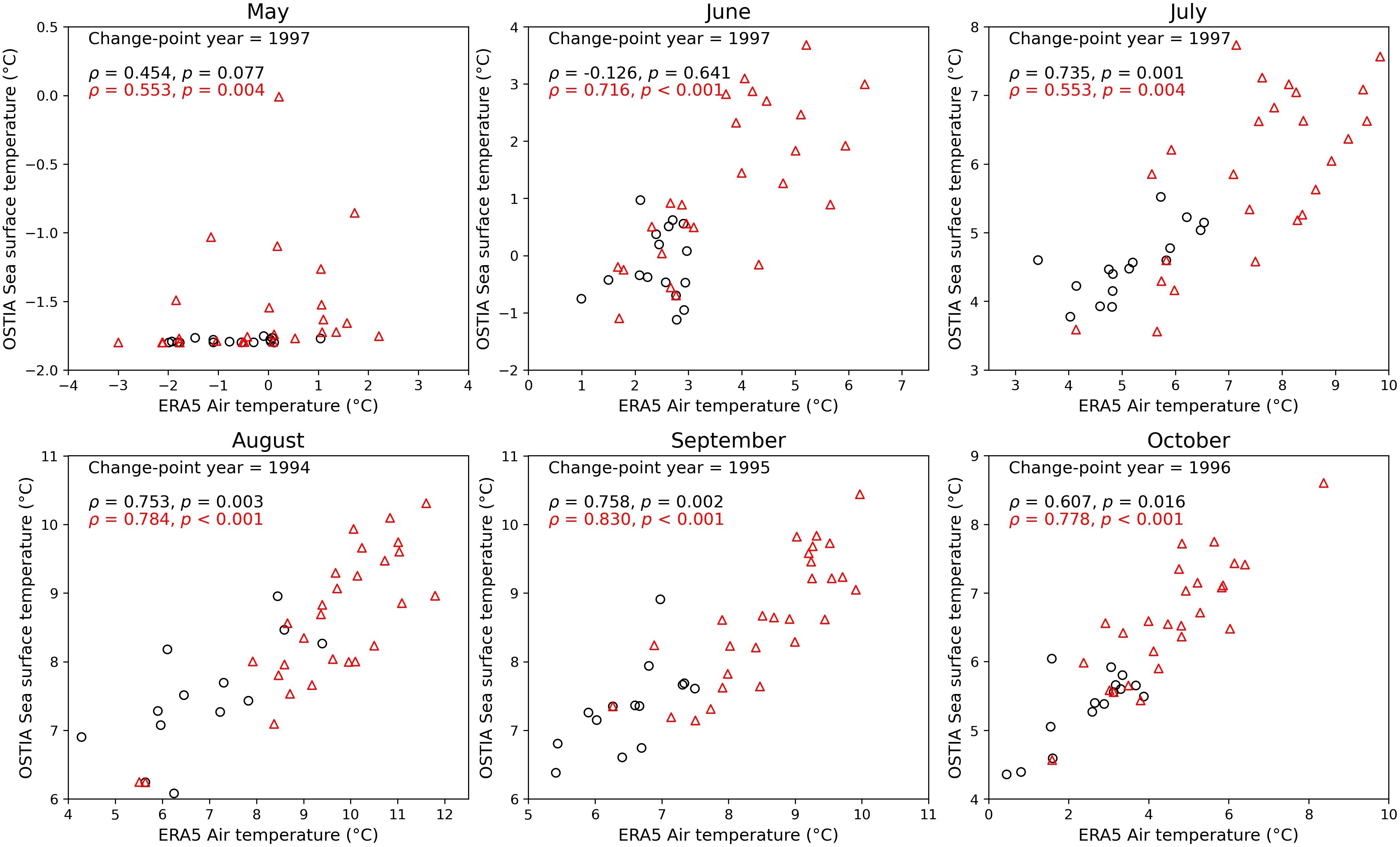
Figure 6. Same as Figure 5 but for SST correlated with ERA 2-m air temperature.

There were also statistically significant positive correlations between the Atlantic Multi-decadal Variability (AMV) index value and SSTs in James Bay (Table 1). There were statistically significant positive correlations between these parameters in each month of our study period, although notably weaker than correlations with ice breakup date and air temperature.

5 Discussion

5.1 Temporal trends in MHWs and a step change in James Bay SSTs over 1982-2021

Similar to other Arctic and sub-Arctic regions where MHW trends have been examined in detail, eastern James Bay has rapidly warmed and seen a dramatic increase in the frequency and intensity of MHWs during the past four decades. The mid- to late-1990s timing of the MHW intensification in James Bay (varying from 1994 to 1997 depending on the month; Figure 4) is similar to or perhaps slightly earlier than Arctic Ocean shelves, which may be expected because of the continental setting and lower latitude the Canadian Inland Seas (Macdonald and Kuzyk, 2011; Ferguson et al., 2010). Baffin Bay, which is also marginal to the Arctic Ocean, underwent a major shift in ice cover and SSTs in 2001 (Ballinger et al., 2022), just slightly later than the changes in James Bay. A few large-scale studies of MHWs in the Arctic and sub-Arctic region have also found evidence of MHWs intensifying in the late 1990s or early 2000s. For example, Thoral et al. (2022) defined 12 coastal biogeographical ‘realms’ across the globe, encompassing the Arctic, north and south Pacific and Atlantic, Indian, and Southern Ocean basins to study MHW trends. For their analysis, the Arctic realm included the sub-Arctic. Using Pettitt change point analysis, they found significant change points in the Arctic realm, with increases in MHW days, number of events, and cumulative intensity since 1998. Huang et al. (2021)’s study of the Arctic realm that focused on areas north of 60°N found a general intensification of MHWs between the early and late parts of the record indicated by, for example, increases in total MHW duration from 13.5 days during 1982–2000 to 28.7 days during 2000–2020. On the other hand, Barkhordarian et al. (2024) emphasized 2007 as being the year of the shift to a “new era of marine heatwaves over the shallow marginal seas of the Arctic Ocean” (p. 7), based in part on a high cumulative intensity of 188°C days for 2007.

Based on the results of the Theil-Sen regression and Pettitt change-point analysis (Figure 4), the warming in eastern James Bay did not occur gradually but rather as an abrupt change or possibly a series of abrupt changes. After only two MHW events during the early portion of the record (1982-1997), five events occurred in 1998 and signaled both an anomalous year and a turning point in the region’s marine climatology. Abrupt shifts in MHWs and underlying SSTs is not uncommon among seasonally ice-covered areas undergoing warming (cf., Ballinger et al., 2022). An abrupt shift in the climatology of SST in James Bay in the mid- to late-1990s (Figure 4), is in agreement with previous studies that have suggested significant change in the coupled atmosphere-ice-ocean system of the Canadian Inland Seas in the late 1990s. Variability in interannual sea ice extent and ice breakup and freeze-up dates is closely related to variation in seasonal surface air temperature and wind in the region (Hochheim and Barber, 2010; Hochheim et al., 2011). Analyzing data from 1980 to 2010, Hochheim and Barber (2014) noted a shift toward warmer surface air temperature anomalies in the mid-1990s during fall and spring (defined by the authors as SON and AMJ, respectively); they further described the period 1996–2005 as “statistically unique” (Hochheim and Barber, 2014, p. 66). An in-depth analysis of SST and ice breakup from 1985 to 2009 conducted by Galbraith and Larouche (2011) found that positive (negative) SST anomalies for the warmest week of the year typically had early (late) ice breakup. The warmest week typically occurred in early to mid-August. In James Bay, they found that the earliest sea-ice breakup occurred in 1998, in early June, which agrees with our analysis.

The regional variability in the timing and rapidity of MHW intensification within the Arctic and sub-Arctic speaks to multiple contributing factors, in addition to Arctic warming. Barkhordarian et al. (2024) found that Arctic MHWs between 1982 and 2022 were primarily triggered by early and abrupt sea-ice retreat which coincided with July maximum downward radiative fluxes. This agrees with our conclusion that part of what intensified MHWs so dramatically in 1998 in James Bay was the exceptionally early ice breakup in May/June.

5.2 Mechanisms leading to MHWs in James Bay

Identifying the physical drivers of MHWs is an active area of research around the globe. For example, Holbrook et al. (2020) outline a range of physical mechanisms that can lead to a MHW event, which include both atmospheric and oceanic preconditioning processes. In a global synthesis of extreme MHW events, Sen Gupta et al. (2020) similarly subdivide the causes of MHW events into 1) changes in ocean heat transport, 2) persistent large-scale atmospheric synoptic systems, and 3) coupled air-sea feedback processes such as El Niño Southern Oscillation (ENSO) events.

5.2.1 Atmospheric preconditioning and ice breakup in James Bay

In our data set, the correlations between SST and variables of ice breakup and air temperature suggest a strong relationship between these parameters, and subsequently to the occurrence of MHWs in the region. Richaud et al. (2024) discussed the complicated interaction between air temperatures, wind and ice in relation to producing MHWs in ice-covered seas, noting that a mobile ice pack can increase wind‐induced vertical mixing of the water column leading to an associated heat flux, yet the direction will be determined by the vertical temperature gradient. Ice-free leads are major sources of surface heat loss during winter but switch over to being sites of surface warming when air temperatures rise during spring. We can also see these complicated interactions in our data.

In the period of each MHW in Figure 2, the ERA5 2-m air temperature was above average (Supplementary Figures S1-S6). However, there were months with statistically significant air temperatures but no MHWs. For example, in May and June in 1982 and 1983, respectively, there were high air temperatures in James Bay but no MHW events. Presumably, this reflects the later ice breakup during those years.

Throughout the period of study, there is a general pattern that years with multiple MHW events had relatively earlier ice breakup (Figure 2), as well as later freeze-up (occurring in December or later). However, it is notable that certain years with early ice breakup (i.e., early June) also had few to no MHW events (e.g., 2006 and 2014). This may be due to the fact that wind, rather than surface air temperature played a larger role in ice breakup in those years (Hochheim and Barber, 2010; Hochheim et al., 2011); thus, while the sea surface would still have increased exposure to incoming solar radiation, stronger winds result in increased mechanical mixing, decreased stratification, and subsequently decreased sea surface temperatures.

The earliest breakup date in the reference period occurred in 1998, the year that saw an increase in the frequency of MHW events. The relationship between earlier ice breakup and increasing SSTs (Figure 5) is unsurprising, given that it allows for longer exposure of the sea surface to incoming solar radiation (Andrews et al., 2018; Crawford et al., 2023). However, ERA5 2-m air temperature also was above average and statistically significant along the northeastern coastline of James Bay in May and June 1998 (Supplementary Figures S1, S2). May 1998 was actually the first statistically significant May air temperature since 1982. Thus, we conclude that warm air temperatures and early ice breakup combined to produce the long-lasting and relatively intense MHW events in May and June 1998. We do not know if other factors such as freshening and shallow stratification related to local riverine discharge or sea-ice melt also played a role.

5.2.2 Winter ENSO events

Mechanisms proposed to explain the Arctic amplification can be loosely divided into remote drivers and local forcings and feedbacks. The latter includes poleward heat and moisture transport resulting from large-scale planetary waves driven by distant sea surface temperature anomalies (McCrystall and Screen, 2021). For example, ENSO has been suggested as a potentially important factor in Arctic climate variability (Jeong et al., 2022).

A major El Niño event is characterized by anomalously warm SSTs that peak in boreal winter in the eastern equatorial Pacific. Jeong et al. (2022) characterized major El Niño events in 1982/1983, 1997/1998, and 2015/2016. The eastern equatorial Pacific SST anomalies were higher than 3°C and the 1997/1998 event saw SSTs average about 2-3°C above normal also off Canada’s Pacific coast (Environment Canada, 1998). During these major El Niño winters, a pattern of cold surface temperatures over the North Pacific can be seen, and substantial warm anomalies over extratropics were highly varied during these three major El Niño winters. Surface air temperatures over the Arctic and Eurasia were anomalously cold in 1997/1998 and warm in 1982/1983, a difference the authors say was likely driven by differences in the lower tropospheric moisture flux in the Arctic leading to cooling and warming, respectively. However, there were anomalously warm surface air temperatures across central Canada during each of these major El Niño events. In particular, while northern Hudson Bay experienced the same anomalously cold surface air temperatures covering most of the Arctic in 1997/1998, the region around southern Hudson Bay and James Bay responded similarly to southern Canada, with winter temperatures about 4-6°C above normal and an unprecedented lack of snow. (An exceptional ice storm that struck southern Canada in January 1998 is remembered because of the 78 mm of ice that built up in Southwestern Québec and led to 34 fatalities, a shutdown of activities in large cities like Montreal and Ottawa, and massive damage to the Hydro- Québec power grid.) Thus, warm winter air temperatures, low snow cover and/or thin ice in James Bay during winter 1997/98 may have preconditioned the coastal marine environment for early ice break-up, which then allowed rapid warming of the surface waters by the atmosphere in May, June, and July 1998.

Two later periods (2010–2012 and 2019-2021) are notable for MHWs that precede full sea ice breakup (Figure 2). In the first period, MHWs persisted throughout the summer in each year; however, the MHWs abated by the end of May in each year of the later period, with only 2021 exhibiting a MHW later in the year. Both 2009/2010 and 2018/2019 were El Niño years, with 2009/2010 being one of three strong El Niño events (ONI ≥ 1.0) since 1998. The most recent, in 2023/2024, also preceded early ice breakup and exceptional MHWs in eastern Hudson Bay, including James Bay (Soriot et al., 2025). The strong El Niño event in winter 2015/2016 was also followed by MHWs in James Bay, although not as many or as strong as 1997/1998 or 2009/2010. The MHW activity in 2019 followed a weaker El Niño event. With only a handful of examples, the differences are not statistically significant, but there is at least preliminary evidence that future of El Niño events (especially strong ones) will increase the likelihood of major MHW events in James Bay the following spring and summer.

5.2.3 Atlantic multi-decadal variability

While El Niño events help explain individual years with frequent MHWs, long-term shifts in MHW frequency require a long-term explanation. The Atlantic Multi-decadal Variability (or AMV) is used to describe SST anomalies on decadal and multi-decadal timescales across most of the Atlantic Ocean (Alexander et al., 2014). Like ENSO, AMV exhibits positive (warmer) and negative (cooler) phases, with differences between these extremes of approximately 0.5°C. The timing of the most recent phase switch varies depending on which SST dataset is used; however, Alexander et al. (2014) describes a positive/warm phase occurring from approximately 1995 to present. Above average SST anomalies in this period occurred in the North Atlantic along the coast of eastern Canada and in Hudson Strait and Hudson Bay (Figure 2e; Alexander et al., 2014).

Prior research has suggested that shifts in AMV have been associated with changes in ecological boundaries, primary productivity, and ecologically and economically important populations across the Atlantic Basin (Nye et al., 2014). Our findings show a consistent relationship between the AMV and SSTs in James Bay (Table 1) and, spatially, significant positive correlations across James Bay from May to October (Supplementary Figure S7), which suggest the influence of atmospheric teleconnections in the region. Little research has been done on the impact of the AMV on the Hudson Bay Complex. Tivy et al. (2011), using canonical correlation analysis for the period 1971 to 2005, found that fall North Atlantic SST explained 69% of the variance in July sea ice concentration in Hudson Bay; the authors hypothesized that this link to the AMV may help explain significant sea ice decline in the Bay since 1979. Ultimately, our results suggest that positive AMV raises the baseline warmth of James Bay – and therefore its susceptibility to MHWs, whereas El Niño events act like a trigger in individual years. Therefore, the AMV index should be an important consideration for future study of MHWs in James Bay.

5.3 Sensitivity of MHW detection and intensity to choice of baselines

The major and abrupt shifts in the climatological baselines in monthly SSTs midway through the study period have implications for how we detect and define MHWs in the James Bay system. Both extreme events and long-term trends affect the average values and the 90^th percentile event-detection threshold. Richaud et al. (2024) discussed this issue in relation to an upward sloping baseline, typical of gradual warming, and suggested that we are less likely to detect MHW events during the early part of the record when we use a long baseline period of 30 years or more. Schlegel et al. (2019) noted that long-term warming trends have greater influence on MHW detection and characterization than the length of the baseline, leading some workers to choose 10- rather than 30- or 40-year baseline periods. In all the preceding Figures and statistics, we used the 90th percentile of the whole 40-year baseline period to identify the MHW events. However, this baseline includes relatively large climatological shifts (i.e., stepwise changes) of more than 1°C for each month of the study (May-October) (Figure 4). Indeed, the average SST in east James Bay for these months combined was 3.86°C in 1982-1997, which is more than was 1°C lower than the average SST of 4.96°C in 1998-2021 (p < 0.01 for a 2-tailed Welch’s t-test).

For east James Bay, we tested how the climatological shifts in SSTs affected the number and intensity of MHW events by recalculating the event statistics using several different baselines. Based purely on statistical considerations, MHW events during the months of May, June, and July should be calculated using two separate shorter baselines (1982–1997 and 1998-2021; Figure 7a and Supplementary Figures S8, S9), to reflect the fact that the climatological baseline for these months shifted in 1997/98. We found that using separate baselines on either side of the change point greatly reduced the disparity in MHW frequency between periods. Using the separate baselines, 59.4% of the MHW days occurred in 1998-2021, compared to 97.7% when using a common baseline of 1982-2021. The 1998–2021 period makes up 60% of the years in the full record, which means the MHW days are almost perfectly proportional between the two periods (1982–1997 and 1998-2021) when using separate baselines. In terms of the number of total MHW days, the switch from using a common baseline to short baselines specific to the early and late periods leads to quite dramatic increases in the total number of MHW days for years in the early part of the record. For example, 1987 (which followed a strong El Niño event) shows an increase from <10 to >30 total MHW days with the short baselines (compare Figures 7a, f).

Figure 7

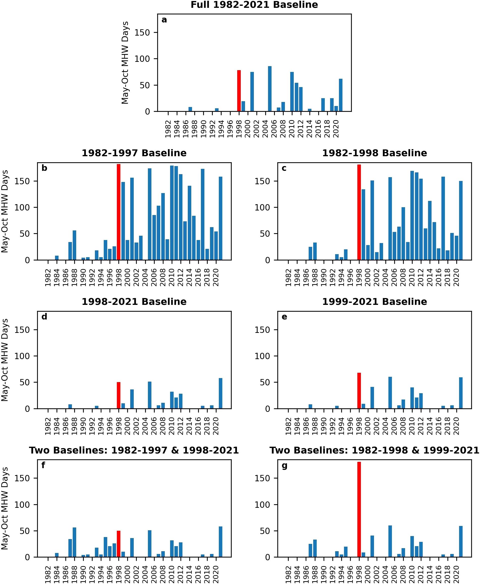
Figure 7. Time series of Marine Heatwave (MHW) Days during May-October in the study area for 1982-2021. Number of MHW days are calculated using (a) the full 1982–2021 period as the baseline for calculating the 90th percentile of sea-surface temperature; (b-e) a shorter period that ends or starts just before/after the climatological shift in 1997/98, but then is applied to the full record; or (f, g) separate baselines for the earlier and later periods in the record. The critical year of 1998 is highlighted in red.

Overall, this analysis means that the abrupt increase in MHW days starting in 1998 can be mostly, if not entirely, attributed to the abrupt increase in average SST in the region. That said, it is also notable that the interannual variability of SST roughly doubled after 1997, from 0.38°C to 0.80°C. Intuitively, this increase in variability would also tend to yield more extremes in the later period, but this emerges from event statistics only if a common baseline is used (1982-2021). With separate baselines for each period, using the 90^th percentile controls for shifts in either the average or the variance. In other words, MHW time series are sensitive to the choice of baseline not only because of sensitivity to the average in SSTs, as discussed by Richaud et al. (2024) and demonstrated here, but also potentially because the 90^th percentile reflects the variance in SSTs.

Although using separate, shorter baselines of 1982–1997 and 1998–2021 makes sense from a climatological standpoint, it is not obvious that this approach makes sense ecologically, where the sequencing of events is relevant. In other words, the magnitude of the MHW intensification that started in 1998 may be better appreciated if it is evaluated relative to the baseline of the period that preceded it, i.e., 1982-1997. Figure 7 and Table 2 show that the number of MHW days in 1998 increases from 78 when the full period is used as the baseline for calculating the 90^th percentile, to 182 MHW days when only the period before the climatological shift (i.e., 1982-1997) is used as the baseline and applied to the full record (compare Figures 7a, b). Using the latter approach, 1998 ranks highest out of the whole study period for the number of MHW days (Table 2), slightly ahead of other high MHW years (2001, 2005, 2010). This contrasts sharply with using two separate periods (1982–1997 and 1998-2021) and having 1998 being compared to a baseline that is strongly influenced by those other high MHW years that came after it. In that case, 1998 ranks fourth overall with 50 MHW days, behind 1988, 2005, and 2021 (Table 2). Other choices of baseline period similarly change the number of MHW days in 1998 and its ranking relative to other high MHW years (Figure 7; Table 2).

Table 2

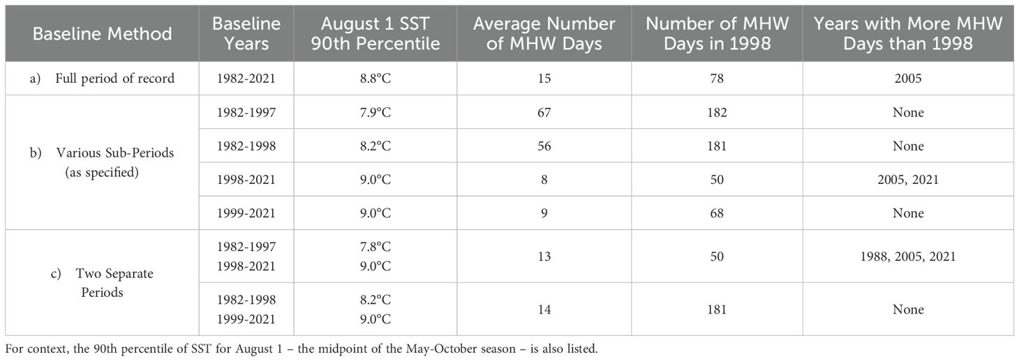
Table 2. Sensitivity of MHW detection and ranking of 1998 to choice of baseline period for calculating the 90th percentile of SST, including: a) using the full period of record to define the 90^th percentiles; b) using various sub-periods to define the 90th percentiles; and c) using two separate baselines to account for the climatological shift.

5.4 Potential ecological significance of MHWs in James Bay

Extreme SSTs associated with MHWs have been shown to impact a wide range of marine species across many different ecoregions (cf., Tolimieri et al., 2023; Smith et al., 2024; Artana et al., 2024; Arteaga and Rousseaux, 2023; Wyatt et al., 2022). Until recently, however, there has been little focus on MHW impacts in the Arctic region. Evidence has now emerged of effects on upper trophic levels, including redistributions of fish communities after successive MHWs in the Barents Sea (Husson et al., 2022) and increased mortality of marine birds after massive reduction in sea ice and prolonged MHWs in the Bering and Chukchi Seas (Jones et al., 2023). Impacts of MHWs on Arctic benthic communities seem likely (cf., Grebmeier et al., 2018) but may remain unknown because of lack of monitoring (and detection and attribution analyses) of coastal marine ecosystems across many parts of the region.

Notably, the 1998 MHW in eastern James Bay coincides with a massive regional seagrass Zostera marina (eelgrass) decline, which it was possible to characterize because of monitoring since 1982, as well as knowledge of local Indigenous Peoples (Cree First Nations; see Fink-Mercier et al., 2024). In investigating environmental factors related to eelgrass abundance, Leblanc and co-workers found statistical associations between low eelgrass biomass and warm SST in June and possible associations with early ice breakup (Leblanc et al., 2023). In east James Bay, it may be that because 1998 was the start of the intensification of MHWs in this region, the MHW events triggered a crash in the ecosystem in 1998-1999. It is already established that there were other precursors to this crash and the ecosystem may have been in a lower-resilience state before change in MHW intensity and frequency (cf., Leblanc et al., 2023). It is well known that local environmental stresses magnify coral loss after marine heatwaves (Donovan et al., 2021) and exacerbates eelgrass loss in regions where other factors such as light reduction and physical disturbance are already causing losses (Plaisted et al., 2022; Lefcheck et al., 2017). The effects of successive intense MHWs after 1998 on the coastal ecosystem are less certain. It may be that single strong (unprecedented) MHWs have more severe impacts than multiple milder MHWs through effects on properties like biodiversity (cf., Liang et al., 2024), but there is also the possibility that successive MHWs, as occurred over 1998-2021, could lead to cumulative impacts, as seen for coral (Bruno et al., 2007), well-studied intertidal species (Harley and Paine, 2009; Siegle et al., 2018), and fish communities (Husson et al., 2022). The eelgrass decline also could be just the tip of the iceberg, with the late-1990s climate shift and step change in MHWs having far-reaching consequences on subarctic marine and coastal ecosystems that have gone undetected scientifically. As pointed out in recent works (e.g., Richaud et al., 2024), it is very important for future ecological studies to consider the impact of extreme events in addition to warming trends; however, this hinges on documentation and analysis of past significant MHW occurrences and their driving processes and careful consideration of the impact of the choice of baselines.

6 Conclusions

Our results demonstrate a dramatic shift in MHW frequency, timing, and duration (see 3.3) in eastern James Bay over the period 1982–2021 as previously postulated for high-latitude regions. The change came abruptly, possibly because of the prolonged and intense winter El Niño in 1997/98. We also find that across the 40-year period of record, MHW intensity in the study area is correlated with ice breakup date as well as air temperature. As ice break-up date shifted from June to May in 1998, ice no longer provided a barrier to atmosphere-ocean heat flux, and air temperature became a primary control on MHWs. Our results highlight the potential for drivers to shift over time as seasonally ice-covered areas lose their sea-ice cover during the shoulder seasons, thus losing this barrier to atmosphere-ocean exchange.

Given projections of a progressively earlier ice breakup in James Bay, more extreme MHWs may be expected during the coming decades and could become pervasive drivers of impacts across a number of marine species and ecosystems. We suggest caution also in using satellite data in a quantitative way to evaluate the intensity of MHW events in coastal habitats, where proximity to land and local features such as the volume of water leaving/entering an estuary or inlet with each tidal cycle (tidal prism) cause high variability and higher temperatures compared to offshore areas. We suggest that continuous measurements of water temperature be included in future coastal monitoring programs alongside parameters of ecosystem health.

Data availability statement

The raw data supporting the conclusions of this article will be made available by the authors, without undue reservation.

Author contributions

JAB: Formal Analysis, Methodology, Visualization, Writing – original draft, Writing – review & editing, Investigation. JKE: Conceptualization, Funding acquisition, Methodology, Supervision, Writing – review & editing. ADC: Formal Analysis, Methodology, Validation, Visualization, Writing – review & editing. MLL: Conceptualization, Methodology, Writing – review & editing. ZZAK: Conceptualization, Methodology, Writing – review & editing, Funding acquisition, Project administration, Supervision.

Funding

The author(s) declare that financial support was received for the research and/or publication of this article. Financial support was received for the research and authorship of this article from ArcticNet, a Network of Centres of Excellence Canada. The Natural Sciences and Engineering Research Council of Canada (NSERC) provided support for research, authorship, and publication. Niskamoon Corporation, a non-profit First Nation organization, provided funds for travel, salary (Leblanc), and project coordination.

Acknowledgments

This research was conducted as part of a large multi-disciplinary project called the Eeyou Coastal Habitat Comprehensive Research Project (CHCRP) (see https://doi.org/10.34992/4K4Z-TF96) coordinated by Niskamoon Corporation. This Cree-driven research project seeks to understand factors affecting the coastal ecosystem especially eelgrass and geese in Eeyou Istchee, eastern James Bay. We thank the Niskamoon local officers and the Cree tallymen and land users for working with us and sharing their knowledge about the coast throughout the project. The manuscript benefited from discussions with fellow academics working within the CHCRP and was much improved by comments provided by Mary O’Connor, University of British Columbia. We also thank the reviewers for comments that improved the manuscript.

Conflict of interest

The authors declare that the research was conducted in the absence of any commercial or financial relationships that could be construed as a potential conflict of interest.

Generative AI statement

The author(s) declare that no Generative AI was used in the creation of this manuscript.

Publisher’s note

All claims expressed in this article are solely those of the authors and do not necessarily represent those of their affiliated organizations, or those of the publisher, the editors and the reviewers. Any product that may be evaluated in this article, or claim that may be made by its manufacturer, is not guaranteed or endorsed by the publisher.

Supplementary material

The Supplementary Material for this article can be found online at: https://www.frontiersin.org/articles/10.3389/fmars.2025.1549329/full#supplementary-material

References

Alexander M. A., Kilbourne K. H., and Nye J. A. (2014). Climate variability during warm and cold phases of the Atlantic Multidecadal Oscillation (AMO) 1871–2008. J. Mar. Syst. 133, 14–26. doi: 10.1016/j.jmarsys.2013.07.017

Crossref Full Text | Google Scholar

Andrews J., Babb D., and Barber D. G. (2018). Climate change and sea ice: Shipping in Hudson Bay, Hudson Strait, and Foxe Basin, (1980–2016). Elem. Sci. Anth. 6, 19. doi: 10.1525/elementa.281

Crossref Full Text | Google Scholar

Artana C., Capitani L., Santos Garcia G., Angelini R., and Coll M. (2024). Food web trophic control modulates tropical Atlantic reef ecosystems response to marine heat wave intensity and duration. J. Anim. Ecol. doi: 10.1111/1365-2656.14107

PubMed Abstract | Crossref Full Text | Google Scholar

Arteaga L. A. and Rousseaux C. S. (2023). Impact of Pacific Ocean heatwaves on phytoplankton community composition. Commun. Biol. 6, 263. doi: 10.1038/s42003-023-04645-0

PubMed Abstract | Crossref Full Text | Google Scholar

Ballinger T. J., Moore G. W. K., Garcia-Quintana Y., Myers P. G., Imrit A. A., Topál D., et al. (2022). Abrupt northern Baffin Bay autumn warming and sea-ice loss since the turn of the twenty-first century. Geophysical Res. Lett. 49, e2022GL101472. doi: 10.1029/2022GL101472

Crossref Full Text | Google Scholar

Barkhordarian A., Nielsen D. M., Olonscheck D., and Baehr J. (2024). Arctic marine heatwaves forced by greenhouse gases and triggered by abrupt sea-ice melt. Commun. Earth Environ. 5, 57. doi: 10.1038/s43247-024-01215-y

Crossref Full Text | Google Scholar

Bruno J. F., Selig E. R., Casey K. S., Page C. A., Willis B. L., Harvell C. D., et al. (2007). Thermal stress and coral cover as drivers of coral disease outbreaks. PloS Biol. 5, e124. doi: 10.1371/journal.pbio.0050124

PubMed Abstract | Crossref Full Text | Google Scholar

Carvalho K. S., Smith T. E., and Wang S. (2021). Bering Sea marine heatwaves: Patterns, trends and connections with the Arctic. J. Hydrology 600, 126462. doi: 10.1016/j.jhydrol.2021.126462

Crossref Full Text | Google Scholar

Chauhan A., Smith P. A. H., Rodrigues F., Christensen A., St. John M., and Mariani P. (2023). Distribution and impacts of long-lasting marine heat waves on phytoplankton biomass. Front. Mar. Sci. 10. doi: 10.3389/fmars.2023.1177571

Crossref Full Text | Google Scholar

C3S CDS (Copernicus Climate Change Service, Climate Data Store) (2021). ORAS5 global ocean reanalysis monthly data from 1958 to present (Copernicus Climate Change Service (C3S) Climate Data Store (CDS).

Google Scholar

Crawford A. D., Rosenblum E., Lukovich J. V., and Stroeve J. C. (2023). Sources of seasonal sea-ice bias for CMIP6 models in the Hudson Bay Complex. Ann. Glaciol. 64, 236-253. doi: 10.1017/aog.2023.42

Crossref Full Text | Google Scholar

Cree Nation of Chisasibi (CNC) (2015). “Migratory birds habitat task force report,” in Chisasibi, Eelgrass, and Waterfowl: A review of Cree traditional ecological knowledge and scientific knowledge(Chisasibi, Québec).

Google Scholar

Davis K. E., Noisette F., Ehn J., Kuzyk Z. A., Peck C. J., and O’Connor M. (2024). Effects of light and water column nutrient availability on eelgrass (Zostera marina) productivity in Eeyou Istchee, eastern James Bay, Quebec. Mar. Ecol. Prog. Ser. 738, 103-117. doi: 10.3354/meps14605

Crossref Full Text | Google Scholar

Davy R. and Griewank P. (2023). Arctic amplification has already peaked. Environ. Res. Lett. 18, 084003. doi: 10.1088/1748-9326/ace273

Crossref Full Text | Google Scholar

de Melo M. L., Gérardin M.-L., Fink-Mercier C., and del Giorgio P. A. (2022). Patterns in riverine carbon, nutrient and suspended solids export to the Eastern James Bay: links to climate, hydrology and landscape. Biogeochem. 161, 291–314. doi: 10.1007/s10533-022-00983-z

Crossref Full Text | Google Scholar

Donlon C. J., Martin M., Stark J., Roberts-Jones J., Fiedler E., and Wimmer W. (2012). The operational sea surface temperature and sea ice analysis (OSTIA) system. Remote Sens. Environ. 116, 140–158. doi: 10.1016/j.rse.2010.10.017

Crossref Full Text | Google Scholar

Donovan M. K., Burkepile D. E., Kratochwill C., Shlesinger T., Sully S., Oliver T. A., et al. (2021). Local conditions magnify coral loss after marine heatwaves. Science 372, 977–980. doi: 10.1126/science.abd9464

PubMed Abstract | Crossref Full Text | Google Scholar

Echavarria-Heras H., Solana-Arellano E., and Franco-Vizcaíno E. (2006). The role of increased sea surface temperature on eelgrass leaf dynamics: onset of El Niño as a proxy for global climate change in San Quintín Bay, Baja California. Bull. - South. Calif. Acad. Sci. 105, 113–127. doi: 10.3160/0038-3872(2006)105[113:TROISS]2.0.CO;2

Crossref Full Text | Google Scholar

Ferguson S., Higdon J., and Chmelnitsky E. (2010). The Rise of Killer Whales as a Major Arctic Predator. In: A Little Less Arctic: Top Predators in the World's Largest Northern Inland Sea, Hudson Bay, Ed. Ferguson S. H., Loseto L. L., and Mallory M. L. (New York, NY, USA: Springer). doi: 10.1007/978-90-481-9121-5_6

Crossref Full Text | Google Scholar

Fink-Mercier C., Leblanc M. L., Noisette F., O’Connor M., Idrobo C. J., Bélanger S., et al. (2024). Cree-driven community-partnered research on coastal ecosystem change in subarctic Canada: a multiple knowledge approach. Arctic Sci. doi: 10.1139/as-2023-0061

Crossref Full Text | Google Scholar

Frölicher T. L. and Laufkötter C. (2018). Emerging risks from marine heat waves. Nat. Commun. 9, 650. doi: 10.1038/s41467-018-03163-6

PubMed Abstract | Crossref Full Text | Google Scholar

Galbraith P. S. and Larouche P. (2011). Sea-surface temperature in Hudson Bay and Hudson Strait in relation to air temperature and ice cover breakup 1985–2009. J. Mar. Syst. 87, 66–78. doi: 10.1016/j.jmarsys.2011.03.002

Crossref Full Text | Google Scholar

Galli G., Solidoro C., and Lovato T. (2017). Marine heat waves hazard 3D maps and the risk for low motility organisms in a warming Mediterranean sea. Front. Mar. Sci. 4. doi: 10.3389/fmars.2017.00136

Crossref Full Text | Google Scholar

Golubeva E., Kraineva M., Platov G., Iakshina D., and Tarkhanova M. (2021). Marine heatwaves in Siberian Arctic seas and adjacent region. Remote Sens. 13. doi: 10.3390/rs13214436

Crossref Full Text | Google Scholar

Good S., Fiedler E., Mao C., Martin M. J., Maycock A., Reid R., et al. (2020). The current configuration of the OSTIA system for operational production of foundation sea surface temperature and ice concentration analyses. Remote Sens. 12. doi: 10.3390/rs12040720

Crossref Full Text | Google Scholar

Grebmeier J. M., Frey K. E., Cooper L. W., and Kędra M. (2018). Trends in benthic macrofaunal populations, seasonal sea ice persistence, and bottom water temperatures in the Bering Strait region. Oceanography 31, 136–151. doi: 10.5670/oceanog.2018.224

Crossref Full Text | Google Scholar

Gupta K., Mukhopadhyay A., Babb D. G., Barber D. G., and Ehn J. K. (2022). Landfast sea ice in Hudson Bay and James Bay: Annual cycle, variability and trends 2000–2019. Elem. Sci. Anth. 10, 73. doi: 10.1525/elementa.2021.00073

Crossref Full Text | Google Scholar

Harley C. D. G. and Paine R. T. (2009). Contingencies and compounded rare perturbations dictate sudden distributional shifts during periods of gradual climate change. Proc. Natl. Acad. Sci. 106, 11172–11176. doi: 10.1073/pnas.0904946106

PubMed Abstract | Crossref Full Text | Google Scholar

Hersbach H., Bell B., Berrisford P., Biavati G., Horányi A., Muñoz Sabater J., et al. (2023). ERA5 hourly data on pressure levels from 1940 to present (Copernicus Climate Change Service (C3S) Climate Data Store (CDS).

Google Scholar

Hobday A. J., Alexander L. V., Perkins S. E., Smale D. A., Straub S. C., Oliver E. C. J., et al. (2016). A hierarchical approach to defining marine heatwaves. Prog. Oceanogr. 141, 227–238. doi: 10.1016/j.pocean.2015.12.014

Crossref Full Text | Google Scholar

Hochheim K. P. and Barber D. G. (2010). Atmospheric forcing of sea ice in Hudson Bay during the fall period 1980–2005. J. Geophys. Res. 115, C05009. doi: 10.1029/2009JC005334

Crossref Full Text | Google Scholar

Hochheim K. P. and Barber D. G. (2014). An update on the ice climatology of the Hudson Bay system. Arct. Antarct. Alp. Res. 46, 66–83. doi: 10.1657/1938-4246-46.1.66

Crossref Full Text | Google Scholar

Hochheim K. P., Lukovich J. V., and Barber D. G. (2011). Atmospheric forcing of sea ice in Hudson Bay during the spring period 1980–2005. J. Mar. Syst. 88, 476–487. doi: 10.1016/j.jmarsys.2011.05.003

Crossref Full Text | Google Scholar

Holbrook N. J., Scannell H. A., Sen Gupta A., Benthuysen J. A., Feng M., Oliver E. C. J., et al. (2019). A global assessment of marine heatwaves and their drivers. Nat. Commun. 10, 1–13. doi: 10.1038/s41467-019-10206-z

PubMed Abstract | Crossref Full Text | Google Scholar

Holbrook N. J., Sen Gupta A., Oliver E. C. J., Hobday A. J., Benthuysen J. A., Scannell H. A., et al. (2020). Keeping pace with marine heatwaves. Nat. Rev. Earth Environ. 1, 482–493. doi: 10.1038/s43017-020-0068-4

Crossref Full Text | Google Scholar

Hu S., Zhang L., and Qian S. (2020). Marine heatwaves in the Arctic region: Variation in different ice covers. Geophys. Res. Lett. 47, e2020GL089329. doi: 10.1029/2020GL089329

Crossref Full Text | Google Scholar

Huang B., Thorne P. W., Banzon V. F., Boyer T., Chepurinm G., Lawrimore J. H., et al. (2017). NOAA Extended Reconstructed Sea Surface Temperature (ERSST), Version 5 (NOAA National Centers for Environmental Information). doi: 10.7289/V5T72FNM

Crossref Full Text | Google Scholar

Huang B., Wang Z., Yin X., Arguez A., Graham G., Liu C., et al. (2021). Prolonged marine heatwaves in the Arctic: 1982–2020. Geophys. Res. Lett. 48, e2021GL095590. doi: 10.1029/2021GL095590

Crossref Full Text | Google Scholar

Huang B., Yin X., Carton J. A., Chen L., Graham G., Liu C., et al. (2023). Understanding differences in sea surface temperature intercomparisons. J. Atmos. Ocean. Tech. 40, 455–473. doi: 10.1175/JTECH-D-22-0081.1

Crossref Full Text | Google Scholar

Hussain M. and Mahmud I. (2019). pyMannKendall: a python package for non-parametric Mann Kendall family of trend tests. J. Open Source Software 4, 1556. doi: 10.21105/joss.01556

Crossref Full Text | Google Scholar

Husson B., Lind S., Fossheim M., Kato-Solvang H., Skern-Mauritzen M., Pécuchet L., et al. (2022). Successive extreme climatic events lead to immediate, large-scale, and diverse responses from fish in the Arctic. Global Change Biol. 28, 3728–3744. doi: 10.1111/gcb.16153

PubMed Abstract | Crossref Full Text | Google Scholar

Idrobo C. J., Leblanc M.-L., and O’Connor M. I. (2024). The “Turning point” for the fall goose hunt in Eeyou Istchee: A social-ecological regime shift from an indigenous knowledge perspective. Hum. Ecol. 52, 617-636. doi: 10.1007/s10745-024-00499-0

Crossref Full Text | Google Scholar

Ingram R. G. and Larouche P. (1987). Changes in the under-ice characteristics of La Grande Rivière plume due to discharge variations. Atmos. Ocean. 25, 242–250. doi: 10.1080/07055900.1987.9649273

Crossref Full Text | Google Scholar

Intergovernmental Panel on Climate Change (IPCC) (2019). IPCC Special Report on the Ocean and Cryosphere in a Changing Climate. Eds. Pörtner H.-O., Roberts D. C., Masson-Delmotte V., Zhai P., Tignor M., Poloczanska E., Mintenbeck K., Alegría A., Nicolai M., Okem A., Petzold J., Rama B., and Weyer N. M. (Cambridge, UK and New York, NY, USA: Cambridge University Press), 755 pp. doi: 10.1017/9781009157964

Crossref Full Text | Google Scholar

Jacox M. G., Alexander M. A., Amaya D., Becker E., Bograd S. J., Brodie S., et al. (2022). Global seasonal forecasts of marine heatwaves. Nature 604, 486–490. doi: 10.1038/s41586-022-04573-9

PubMed Abstract | Crossref Full Text | Google Scholar

Jarrin M., Jose M., Sutherland D. A., and Helms A. R. (2022). Water temperature variability in the Coos Estuary and its potential link to eelgrass loss. Front. Mar. Sci. 9. doi: 10.3389/fmars.2022.930440

Crossref Full Text | Google Scholar

Jenkins M. and Dai A. (2021). The impact of sea-ice loss on arctic climate feedbacks and their role for arctic amplification. Geophys. Res. Lett. 48. doi: 10.1029/2021gl094599

Crossref Full Text | Google Scholar

Jeong H., Park H.-S., Malte F. Stuecker M. F., and Yeh S.-W. (2022). Distinct impacts of major El Niño events on Arctic temperatures due to differences in eastern tropical Pacific sea surface temperatures. Sci. Adv. 8. doi: 10.1126/sciadv.abl8278

PubMed Abstract | Crossref Full Text | Google Scholar

Johnson M. R., Williams S. L., Lieberman C. H., and Solbak A. (2003). Changes in the abundance of the seagrasses Zostera marina L. (eelgrass) and Ruppia maritima L. (widgeongrass) in San Diego, California, following an El Niño Event. Estuaries Coast. 26, 106. doi: 10.1007/BF02691698

Crossref Full Text | Google Scholar

Jones T., Parrish J. K., Lindsey J., Wright C., Burgess H., Dolliver J., et al. (2023). Marine bird mass mortality events as an indicator of the impacts of ocean warming. Marine Ecology Progress Series HEAT. doi: 10.3354/meps14330

Crossref Full Text | Google Scholar

Lalumière R., Messier D., Fournier J.-J., and McRoy P. C. (1994). Eelgrass meadows in a low arctic environment, the northeast coast of James Bay, Québec. Aquat. Bot. 47, 303–315. doi: 10.1016/0304-3770(94)90060-4

Crossref Full Text | Google Scholar

Lannuzel D., Tedesco L., van Leeuwe M., Campbell K., Flores H., Delille B., et al. (2020). The future of Arctic sea-ice biogeochemistry and ice-associated ecosystems. Nat. Climate Change 10, 983–992. doi: 10.1038/s41558-020-00940-4

Crossref Full Text | Google Scholar

Leblanc M.-L., O’Connor M. I., Kuzyk Z. A., Noisette F., Davis K. E., Rabbitskin E., et al. (2023). Limited recovery following a massive seagrass decline in sub-Arctic eastern Canada. Glob. Change Biol. 29, 432–450. doi: 10.1111/gcb.16499

PubMed Abstract | Crossref Full Text | Google Scholar

Lefcheck J. S., Wilcox D. J., Murphy R. R., Marion S. R., and Orth R. J. (2017). Multiple stressors threaten the imperiled coastal foundation species eelgrass (Zostera marina) in Chesapeake Bay, USA. Glob. Change Biol. 23, 3474–3483. doi: 10.1111/gcb.13623

PubMed Abstract | Crossref Full Text | Google Scholar

Liang M., Lamy T., Reuman D. C., Wang S., Bell T. W., Cavanaugh K. C., et al. (2024). A marine heatwave changes the stabilizing effects of biodiversity in kelp forests. Ecology 105, e4288. doi: 10.1002/ecy.4288

PubMed Abstract | Crossref Full Text | Google Scholar

Macdonald R. W. and Kuzyk Z. A. (2011). The Hudson Bay system: A northern inland sea in transition. J. Mar. Syst. 88, 337–340. doi: 10.1016/j.jmarsys.2011.06.003

Crossref Full Text | Google Scholar

McCrystall M. R. and Screen J. A. (2021). Arctic winter temperature variations correlated with ENSO are dependent on coincidental sea ice changes. Geophys. Res. Lett. 48, e2020GL091519. doi: 10.1029/2020GL091519

Crossref Full Text | Google Scholar

McDonald M., Arragutainaq L., and Novalinga Z. (1997). Voices from the Bay: Traditional Ecological Knowledge of Inuit and Cree in the Hudson Bay Bioregion (Ottawa, Ontario: Canadian Arctic Resources Committee and Environmental Committee of the Municipality of Sanikiluaq).

Google Scholar

Messier D., Lepage S., and de Margerie S. (1989). Influence du couvert de glace sur l’étendue du panache de la Grande Rivière (baie James). Arctic 42, 278–284. doi: 10.14430/arctic1666

Crossref Full Text | Google Scholar

Mohamed B., Nilsen F., and Skogseth R. (2022). Marine heatwaves characteristics in the Barents Sea based on high resolution satellite data, (1982–2020). Front. Mar. Sci. 9. doi: 10.3389/fmars.2022.821646

Crossref Full Text | Google Scholar

Nye J. A., Baker M. R., Bell R., Kenny A., Kilbourne K. H., Friedland K. D., et al. (2014). Ecosystem effects of the Atlantic Multidecadal Oscillation. J. Mar. Syst. 133, 103–116. doi: 10.1016/j.jmarsys.2013.02.006

Crossref Full Text | Google Scholar

Oliver E. C. J., Benthuysen J. A., Darmaraki S., Donat M. G., Hobday A. J., Holbrook N. J., et al. (2021). Marine heatwaves. Ann. Rev. Mar. Sci. 13, 313–342. doi: 10.1146/annurev-marine-032720-095144

PubMed Abstract | Crossref Full Text | Google Scholar

Peck C. J., Kuzyk Z. A., Heath J. P., Lameboy J., and Ehn J. K. (2022). Under-ice hydrography of the La Grande river plume in relation to a ten-fold increase in wintertime discharge. J. Geophys. Res. Oceans 127, e2021JC018341. doi: 10.1029/2021JC018341

Crossref Full Text | Google Scholar

Plaisted H. K., Shields E. C., Novak A. B., Peck C. P., Schenck F., Carr J., et al. (2022). Influence of rising water temperature on the temperate seagrass species eelgrass (Zostera marina L.) in the northeast USA. Front. Mar. Sci. 9. doi: 10.3389/fmars.2022.920699

Crossref Full Text | Google Scholar

Prinsenberg S. J. (1986a). “Chapter 10 the circulation pattern and current structure of hudson bay,” in Elsevier Oceanography Series. Ed. Martini I. P. (New York, NY, USA: Elsevier), 187–204.

Google Scholar

Prinsenberg S. J. (1986b). “Chapter 9 salinity and temperature distributions of Hudson Bay and James Bay,” in Elsevier Oceanography Series. Ed. Martini I. P. (New York, NY, USA: Elsevier), 163–186.

Google Scholar

Richaud B., Hu X., Darmaraki S., Fennel K., Lu Y., and Oliver E. C. J. (2024). Drivers of marine heatwaves in the Arctic Ocean. J. Geophys. Res. Oceans 129, e2023JC020324. doi: 10.1029/2023JC020324

Crossref Full Text | Google Scholar

Ridenour N. A., Hu X., Jafarikhasragh S., Landy J. C., Lukovich J. V., Stadnyk T. A., et al. (2019). Sensitivity of freshwater dynamics to ocean model resolution and river discharge forcing in the Hudson Bay Complex. J. Mar. Syst. 196, 48–64. doi: 10.1016/j.jmarsys.2019.04.002

Crossref Full Text | Google Scholar

Russo E. and Domeisen D. I. V. (2023). Increasing intensity of extreme heatwaves: The crucial role of metrics. Geophys. Res. Lett. 50, e2023GL103540. doi: 10.1029/2023GL103540

Crossref Full Text | Google Scholar

Schlegel R. W., Oliver E. C. J., Hobday A. J., and Smit A. J. (2019). Detecting marine heatwaves with sub-optimal data. Front. Mar. Sci. 6. doi: 10.3389/fmars.2019.00737

Crossref Full Text | Google Scholar

Sen Gupta A., Thomsen M., Benthuysen J. A., Hobday A. J., Oliver E., Alexander L. V., et al. (2020). Drivers and impacts of the most extreme marine heatwave events. Sci. Rep. 10, 19359. doi: 10.1038/s41598-020-75445-3

PubMed Abstract | Crossref Full Text | Google Scholar

Serreze M. C. and Barry R. G. (2011). Processes and impacts of Arctic amplification: A research synthesis. Global Planet Change 77, 85–96. doi: 10.1016/j.gloplacha.2011.03.004

Crossref Full Text | Google Scholar

Serreze M. C. and Meier W. N. (2019). The Arctic’s sea ice cover: trends, variability, predictability, and comparisons to the Antarctic. Ann. N.Y. Acad. Sci. 1436, 36–53. doi: 10.1111/nyas.13856

PubMed Abstract | Crossref Full Text | Google Scholar

Siegle M. R., Taylor E. B., and O’Connor M. I. (2018). Prior heat accumulation reduces survival during subsequent experimental heat waves. J. Exp. Mar. Biol. Ecol. 501, 109–117. doi: 10.1016/j.jembe.2018.01.012

Crossref Full Text | Google Scholar

Smith K. E., Aubin M., Burrows M. T., Filbee-Dexter K., Hobday A. J., Holbrook N. J., et al. (2024). Global impacts of marine heatwaves on coastal foundation species. Nature Communications 15 (1), 5052. doi: 10.1038/s41467-024-49307-9

PubMed Abstract | Crossref Full Text | Google Scholar

Soriot C., Stroeve J., and Crawford A. (2025). Record early sea ice loss in southeastern Hudson Bay in Spring 2024. Geophys. Res. Lett. 52. doi: 10.1029/2024gl112584

Crossref Full Text | Google Scholar

Stadnyk T. A., Tefs A., Broesky M., Déry S. J., Myers P. G., Ridenour N. A., et al. (2021). Changing freshwater contributions to the Arctic: A 90-year trend analysis (1981–2070). Elementa: Science of the Anthropocene 9 (1), 00098. doi: 10.1525/elementa.2020.00098

Crossref Full Text | Google Scholar

Stroeve J., Crawford A., Ferguson S., Stirling I., Archer L., York G., et al. (2024). Ice-free period too long for Southern and Western Hudson Bay polar bear populations if global warming exceeds 1.6 to 2.6°C. Commun. Earth Environ. 5, 296. doi: 10.1038/s43247-024-01430-7

Crossref Full Text | Google Scholar

Suursaar U. (2022). Summer 2021 marine heat wave in the Gulf of Finland from the perspective of climate warming. Est. J. Earth Sci. 71 1–16. doi: 10.3176/earth.2022.01

Crossref Full Text | Google Scholar

Taha W., Bonneau-Lefebvre M., Cueto Bergner A., and Tremblay A. (2019). Evolution from past to future conditions of fast ice coverage in James Bay. Front. Earth Sci. 7. doi: 10.3389/feart.2019.00254

Crossref Full Text | Google Scholar

Thoral F., Montie S., Thomsen M. S., Tait L. W., Pinkerton M. H., and Schiel D. R. (2022). Unravelling seasonal trends in coastal marine heatwave metrics across global biogeographical realms. Sci. Rep. 12, 7740. doi: 10.1038/s41598-022-11908-z

PubMed Abstract | Crossref Full Text | Google Scholar

Tivy A., Howell S. E. L., Alt B., Yackel J. J., and Carrieres T. (2011). Origins and levels of seasonal forecast skill for sea ice in Hudson Bay using canonical correlation analysis. J. Climate 24, 1378–1395. doi: 10.1175/2010JCLI3527.1

Crossref Full Text | Google Scholar

Tolimieri N., Shelton A. O., Samhouri J. F., Harvey C. J., Feist B. E., Williams G. D., et al. (2023). Changes in kelp forest communities off Washington, USA, during and after the 2014–2016 marine heatwave and sea star wasting syndrome. Mar. Ecol. Prog. Ser. 703, 47–66. doi: 10.3354/meps14220

Crossref Full Text | Google Scholar

UK Met Office (2012). OSTIA L4 SST Analysis (GDS2). Ver. 2.0 (CA, USA: PO. DAAC).

Google Scholar

Wernberg T., Thomsen M. S., Baum J. K., Bishop M. J., Bruno J. F., Coleman M. A., et al. (2024). Impacts of climate change on marine foundation species. Ann. Rev. Mar. Sci. 16, 247–282. doi: 10.1146/annurev-marine-042023-093037

PubMed Abstract | Crossref Full Text | Google Scholar

Worden E., Pearce T., Gruben M., Ross D., Kowana C., and Loseto L. (2020). Social-ecological changes and implications for understanding the declining beluga whale (Delphinapterus leucas) harvest in Aklavik, Northwest Territories. Arctic Sci. 6, 229–246. doi: 10.1139/as-2019-0027

Crossref Full Text | Google Scholar

Wyatt A. M., Resplandy L., and Marchetti A. (2022). Ecosystem impacts of marine heat waves in the Northeast Pacific. Biogeosciences 19, 5689–5705. doi: 10.5194/egusphere-2022-17

Crossref Full Text | Google Scholar

Zhang X. J., Zheng F., Zhu J., and Chen X. R. (2022). Observed frequent occurrences of marine heatwaves in most ocean regions during the last two decades. Adv. Atmos. Sci. 39, 1579–1587. doi: 10.1007/s00376-022-1291-3

Crossref Full Text | Google Scholar