A novel method for distinguishing different algal blooms in the East China Sea via geostationary ocean color satellite observations

Introduction: Dinoflagellate and diatom blooms are the most frequent marine ecological disasters in the Yangtze River estuary (YRE) and adjacent areas of the East China Sea (ECS). Distinguishing between these bloom types is essential for accurate monitoring and effective mitigation.

Methods: To investigate the physiological differences between bloom types, algal culture experiments were conducted to quantify variations in fluorescence quantum yield (φ) between dinoflagellates and diatoms during the growth phase. Using insights from the experiments, an identification and classification method for harmful algal blooms (HABs) was developed based on Geostationary Ocean Color Imager-II (GOCI-II) data. The method incorporates the difference in remote sensing reflectance (Rrs) between the fluorescence peak and baseline bands and establishes a φ-based classification threshold.

Results: Validation of GOCI-II Level-2 products showed that fluorescence-band Rrs products have high accuracy and strong correlation with in situ measurements. A threshold of φ = 0.014 was proposed to distinguish dinoflagellate from diatom blooms. The derived methods were successfully applied to GOCI-II imagery, enabling precise detection and classification of HABs in ECS waters.

Discussion: The proposed approach demonstrated strong capability for monitoring the spatial distribution and evolution of HABs. It provides a reliable technique for distinguishing bloom types using geostationary satellite data, offering valuable support for marine environmental management and mitigation efforts.

1 Introduction

In recent years, as eutrophication in the coastal oceans has intensified, the frequency and scale of harmful algal blooms (HABs) have continuously increased. The areas in the East China Sea (ECS) susceptible to HABs are optically complex case-II waters influenced by multiple factors, including the Yangtze River estuary (YRE), the Taiwan Warm Current, and the Kuroshio region, as well as sea areas affected by regional climate change (Tang et al., 2006; Li et al., 2010; Wang and Wu, 2009). According to the Bulletin of China Marine Disasters issued by the Ministry of Natural Resources of the People’s Republic of China, HABs in the ECS occur almost every year (as shown in Figure 1) between April and October and are primarily driven by diatoms and dinoflagellates (Shen et al., 2019; Zhou et al., 2017). In the ECS, large-scale blooms dominated by Prorocentrum donghaiense (P. donghaiense) occur every late spring and early summer, while other types of blooms dominated by diatoms, such as Skeletonema costatum (S. costatum), also occur frequently (Xiao et al., 2018; Guo et al., 2014). The outbreak of HABs disrupts the marine ecological balance, causes significant economic losses in the marine sector of China, and can even result in casualties (Sanseverino et al., 2016; Guan et al., 2022). Therefore, comprehensively understanding the timing, spatial distribution, scale, and dominant algal species of algal bloom events, as well as elucidating the mechanisms behind their occurrence, is crucial for monitoring and managing HABs (Anderson et al., 2012; Peng et al., 2024; Anderson et al., 2019). However, the sudden nature of HABs and the complexity of their formation make it difficult to predict and forecast these events and to classify the dominant algal species. Thus, clarifying the physiological characteristics of phytoplankton can improve the accuracy of algal bloom monitoring.

Figure 1

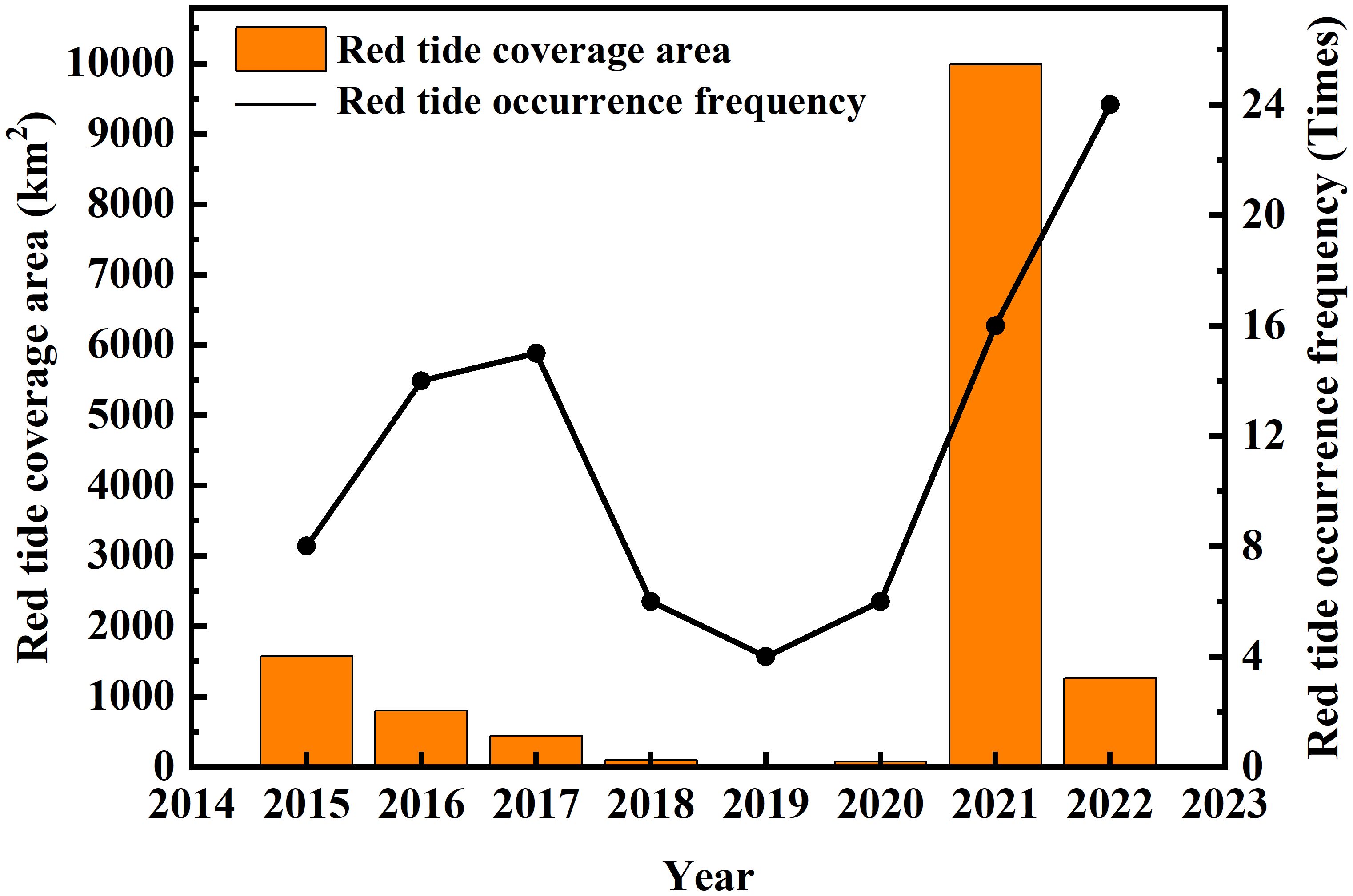
Figure 1. Frequency and area of HABs in the ECS from 2015 to 2022 (source: Bulletin of China Marine Disasters).

Currently, research on the monitoring and classification of HABs and algal species in the ECS has significantly advanced. Young and Frank (1996) used Moderate Resolution Imaging Spectroradiometer (MODIS) fluorescence products to differentiate between algal bloom waters, specifically distinguishing between blooms of Cochlodinium polykrikoides and nonbloom waters. Siswanto et al. (2013) effectively distinguished between Karenia mikimotoi (K. mikimotoi) blooms, diatom blooms, chromophoric dissolved organic matter (CDOM), and water bodies dominated by a mix of substances via MODIS remote sensing imagery. Tao et al. (2015) proposed the ECS dinoflagellate index and the diatom index based on MODIS data and suggested a threshold of 555 nm for the remote sensing reflectance to differentiate between diatom and P. donghaiense blooms. Shang et al. (2014) quantified the inherent optical properties of two common algal species in ECS blooms (P. donghaiense and S. costatum) through laboratory measurements and employed MODIS fluorescence line height (FLH) products to determine the presence of these algal species. In 2017, Hu and Feng (2017) improved the MODIS FLH algorithm and used the improved version to assess algal bloom conditions. Orlova et al. (2022) identified the logarithmic phase, plateau phase, and dominant algal species succession of blooms via the ratio of the FLH concentration to the chlorophyll a (Chl a) concentration and reported that an environmental disaster in the Kamchatka Peninsula in the fall of 2020 was caused by a large-scale bloom of harmful microalgae from the genus Karenia.

Phytoplankton chloroplasts can reduce notable light damage by emitting fluorescence, thereby avoiding the absorption of light energy beyond what is needed for photosynthesis. Therefore, the fluorescence intensity of phytoplankton is closely related to their biomass and photosynthetic process (Murchie and Lawson, 2013; Ralph et al., 2015; Falkowski and Kolber, 1995). The most representative phytoplankton fluorescence parameter is the fluorescence quantum yield (φ). Notably, φ refers to the ratio of the number of fluorescence photons emitted by phytoplankton after absorbing solar photons to the total number of solar photons absorbed (Behrenfeld et al., 2009; Maxwell and Johnson, 2000). In particular, φ can reflect information on the light intensity, nutritional status, and species composition, providing a noninvasive estimate of the physiological and ecological processes of phytoplankton (Lichtenthaler and Rinderle, 1988).

Different algal species exhibit significant differences in φ throughout their growth and decay processes, with substantial variations in absolute values and cyclical changes. For an example, Goodwin explained that the remote sensing-based φ can be used to monitor the photophysical biological status of phytoplankton on a global scale (Goodwin, 2011). Moreover, φ is closely related to the physiological state of phytoplankton and characterizes the strength of photosynthesis. The differences in φ at various stages of the growth and decay cycles of different algal species can be substantial (Zhao et al., 2022; Bannister and Weidemann, 1984). Compared with chlorophyll concentration products commonly applied in ocean color remote sensing, φ contains more information on phytoplankton physiological states and is an effective tool for algal bloom monitoring and the classification of dominant algal species. However, research on the application of φ is limited. Studies involving the use of satellite remote sensing to detect phytoplankton fluorescence signals have focused mainly on deriving chlorophyll concentrations from fluorescence signals without fully utilizing the significant differences in φ at various stages of the growth and decay cycles for algal species classification and bloom prediction. This study aimed to quantify the differences in φ between dinoflagellate and diatom blooms at their growth stages base on algal culture experiments and to develop methods for identifying and classifying algal bloom waters suitable for Geostationary Ocean Color Imager-II (GOCI-II) data.

2 Data and methods

2.1 Study area and measurement data

The primary study area is the ECS, which is a region frequently affected by algal bloom disasters. The ECS is located in eastern China, geographically spanning from 23°00’ to 33°10’ N latitude and 117°11’ to 131°00’ E longitude. It borders the Sea of Japan to the northeast, the Taiwan Strait to the southwest, and the Yellow Sea to the northwest. As an important marine economic and strategic area of China, it covers an area of approximately 770,000 square kilometers with an average seawater depth of 73 m (Domrös and Peng, 2012).

Since 1989, the Ministry of Natural Resources of China has compiled statistics on the occurrence of algal blooms along the Chinese coast (https://ecs.mnr.gov.cn). Information such as the time, location, spatial extent, and dominant species of blooms is collected and published in the Bulletin of China Marine Disasters (http://www.nmdis.org.cn/hygb/zghyhjzlgb/). Data for the bulletin are obtained through annual cruises, fixed stations, and buoy surveys to monitor the marine environment of the ECS. Algal bloom events are recorded during simultaneous surveys conducted by ships and aircraft. The regions, extents, and durations of these events are approximately estimated, and the dominant algal species involved are identified. In this study, we collected records of algal bloom events from the Bulletin of China Marine Disasters from 2021 to 2023. We selected those events that occurred under clear weather conditions (as indicated in Table 1; Figure 2) to validate the algorithms employed in this research. This study utilizes algal bloom events with minimal cloud cover and available satellite data.

Table 1

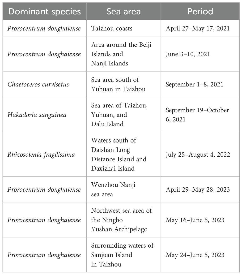
Table 1. Algal bloom disasters occurrence areas and times in parts of the ECS.

Figure 2

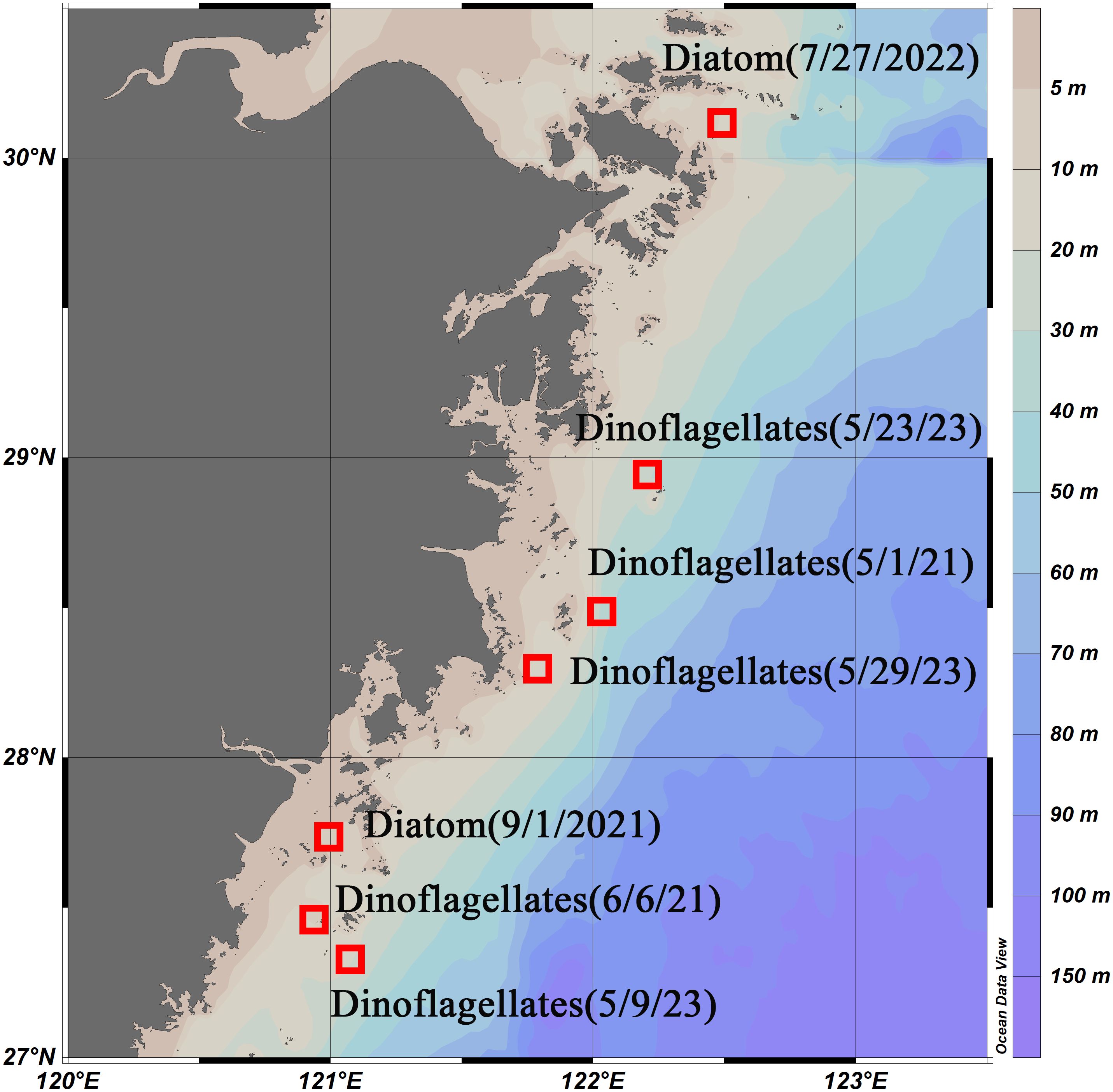
Figure 2. Selected regions and outbreak times of dinoflagellate and diatom blooms.

To ensure the accuracy of GOCI-II ocean color remote sensing products for use in the coastal waters of the ECS for subsequent research, two field experiments were conducted along the coast oceans of the Zhejiang province. The distribution of the cruise stations is shown in Figure 3, spanning from November 9-10, 2021, and April 9-18, 2024. Measurements were obtained under clear weather conditions, resulting in a total of 28 sets of spectral data. The remote sensing reflectance (Rrs) was measured via a portable field spectroradiometer manufactured by the American ASD company. (spectral range, 350–2500 nm; spectral resolution, 3 nm). The measurement method followed the ocean optics protocols of NASA (Mueller et al., 2003). The Rrs value can be calculated using Equation 1.

Figure 3

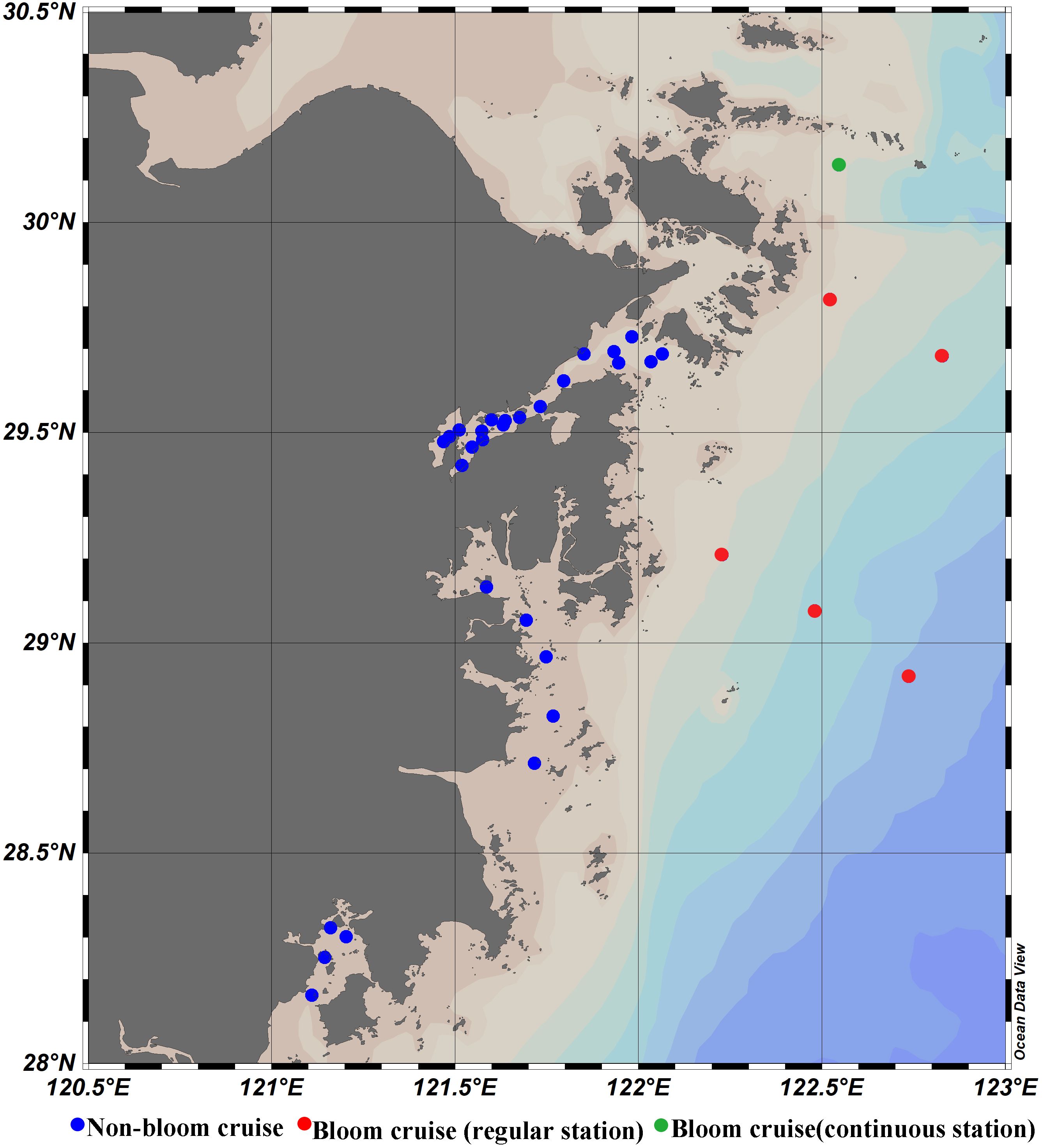
Figure 3. Map of the location of the sampling sites along the ECS coast for the 2019, 2021 and 2024 cruises.

$\begin{array}{ll}{\text{ R}}_{\text{rs}}=\frac{\text{r}({\text{L}}_{\text{t}}-{\text{L}}_{\text{s}}*\text{ρ})}{{\text{πL}}_{\text{r}}}& (1)\end{array}$

where ${\text{L}}_{\text{t}}$ is the upward radiance above the water surface; ${\text{L}}_{\text{s}}$ is the downwelling radiance of the sky; r is the reflectance of the reference panel; ${\text{L}}_{\text{r}}$ is the upward radiance of the reference panel, and ρ is the surface reflectance with the value of 0.028 (He et al., 2013).

Additionally, in-situ data from the 2019 cruise, conducted from April 29 to May 5, were used to validate the algorithm developed in this study, thereby enhancing the algorithm’s reliability. During this cruise, a dinoflagellate bloom occurred in the region (also reported in the 2019 Bulletin of China Marine Disasters). The sampling sites are marked in Figure 3, with green dots representing continuous monitoring stations, where measurements were taken 10 times throughout the day from 8:30 AM to 4:30 PM. The remaining sites (red dots) were sampled twice per hour, for a total of 20 measurements.

2.2 Satellite data

GOCI-II data were obtained from the National Ocean Satellite Center (https://www.nosc.go.kr/eng/main.do). The atmospheric correction method for the Rrs products was based on the algorithm developed by Ahn et al. (2016). In this algorithm, the spectral relationships of multiple scattering reflections of aerosols between different wavelengths (referred to as SRAMS) are used to directly calculate the multiple scattering reflectance contributions of selected aerosol models in the near-infrared bands. Moreover, Chl a products were derived from the inversion results of the OC4 algorithm (O’Reilly et al., 1998).

The spatiotemporal matching between in-situ data and satellite data was conducted using the average value of valid pixels within a 3×3 pixel region centered on the in-situ sampling point, with a time window of ±1 hour for available data (Li et al., 2020). Additionally, the following conditions must be met:

1. The percentage of valid pixels within the 3×3 window (excluding land pixels) was checked. If the percentage exceeded 50%, the window was used for subsequent accuracy validation.

2. The mean and standard deviation of valid Rrs values within the window were calculated. Pixels with Rrs values outside the range of the mean ±1.5 times the standard deviation were discarded.

3. The mean and standard deviation of the remaining valid pixels were recalculated, and the coefficient of variation (CV, standard deviation divided by the mean) was computed to assess spatial heterogeneity. If the CV was less than 0.15, the window was used to match the in-situ data with the satellite data.

The accuracy assessment of the satellite Rrs product was based on the following statistical parameters: root mean square deviation (RMSD), absolute percentage deviation (APD), and relative percentage deviation (RPD). The RMSD,APD and RPD can be calculated using Equations 2–4 respectively.

$\begin{array}{ll}\text{RMSD}=\sqrt{\frac{{\sum }_{\text{i}=1}^{\text{N}}{({\text{Y}}_{\text{i}}-{\text{X}}_{\text{i}})}^2}{\text{N}}}& (2)\end{array}$

$\begin{array}{ll}\text{APD}=100\%*\frac{1}{\text{N}}*{\sum }_{\text{i}=1}^{\text{N}}\frac{|{\text{Y}}_{\text{i}}-{\text{X}}_{\text{i}}|}{{\text{X}}_{\text{i}}}& (3)\end{array}$

$\begin{array}{ll}\text{RPD}=100\%*\frac{1}{\text{N}}*{\sum }_{\text{i}=1}^{\text{N}}\frac{{\text{Y}}_{\text{i}}-{\text{X}}_{\text{i}}}{{\text{X}}_{\text{i}}}& (4)\end{array}$

Here, Y_i, X_i, and N represent the algorithm-retrieved value, the in-situ measured value, and the number of samples, respectively. The RPD indicates the systematic error or the predictive metric of the average relative deviation, while the APD reflects the absolute accuracy of the retrieved product relative to the in-situ data.

2.3 Algal culture experiments

To quantify the differences in fluorescence signals during the growth of different algal species, algal cultures were conducted. In these experiments, different algal species were placed in transparent culture buckets within a constant-temperature circulating water bath. The content of Chl a in the algal solution was measured daily via a Turner fluorometer, and the algal cell density was calculated via optical microscopy. The growth stages of phytoplankton were determined on the basis of changes in the Chl a concentration and cell density. Additionally, the fluorescence intensity at the chlorophyll emission peak was measured via a fluorescence spectrophotometer, and the phytoplankton absorption coefficient was measured via a UV spectrophotometer. The ratio of these two measurements was used to calculate the actual φ value of phytoplankton (Behrenfeld et al., 2009). The main steps are as follows:

I. Both experimental algae were obtained from the Jiangsu Provincial Key Laboratory of Marine Biotechnology at Jiangsu Ocean University in Lianyungang City, Jiangsu Province, China. These algal strains were cultured in 200 mL Erlenmeyer flasks containing sterilized seawater enriched with modified f/2 medium. The culture conditions were maintained at a temperature of 23 ± 1°C, salinity of 35, pH of 8.0 ± 0.2, and light intensity of 4000 lux with a 12:12 h light-dark cycle. The flasks were shaken three times daily to prevent the algal cells from settling and aggregating at the bottom, which could impede their growth., and the flasks were shaken to prevent algal cells from settling at the bottom, which could affect growth.

II. In a sterile environment, a suitable amount of penicillin was added to the algal mixture during the logarithmic growth phase, followed by the addition of streptomycin sulfate and kanamycin sulfate within 24 hours to remove contaminants. After the algal cells reached the logarithmic growth phase, they were inoculated four times into new Erlenmeyer flasks to activate the cells. Logarithmic-phase algal cells were then inoculated into transparent PVC culture buckets containing sterilized seawater with a culture medium in a constant-temperature circulating water bath. Each species was cultured in two parallel setups and grown under suitable conditions involving natural light exposure and daily shaking.

III. The algal solutions were sampled via centrifuge tubes daily, and the algal cell density was measured via optical microscopy, after which the results were averaged to determine the growth stage on the basis of the cell density. The fluorescence intensity at the emission peak was measured via a fluorescence spectrophotometer.

IV. The chlorophyll concentration was measured daily via a filtration method, and the spectral curve of the algal mixture was measured via a portable field spectroradiometer.

2.4 Algal bloom water identification method

In this study, the developed algorithm was compared with three widely used algal bloom water identification methods for processing satellite data.

2.4.1 Red tide index method

The red tide index (RI) (Lou and Hu, 2014) is a commonly used method for identifying algal bloom waters in the ECS. In this method, an additional band in the blue/green ratio is used to suppress the interference of sediments in the algal bloom detection algorithm. Research has indicated that the RI can be applied to detect HABs via geostationary ocean color imager (GOCI) data. The RI was calculated via the Rrs value at 443, 490, and 555 nm, with an RI value above 2.8 indicating algal bloom water.

The RI can be calculated using Equation 5.

$\begin{array}{ll}\text{RI}=\frac{{\text{R}}_{\text{rs}}(555)-{\text{R}}_{\text{rs}}(443)}{{\text{R}}_{\text{rs}}(490)-{\text{R}}_{\text{rs}}(443)}& (5)\end{array}$

2.4.2 Spectral shape method

The spectral shape (SS) method (Wynne et al., 2008) aims to distinguish between bloom and nonbloom waters by analyzing changes in the spectral shape of satellite sensor imagery in the 680 nm band. When the SS index is negative, this indicates an algal bloom. The SS can be calculated using Equation 6.

$\begin{array}{ll}\text{SS}(680)={\text{R}}_{\text{rs}}(680)-{\text{R}}_{\text{rs}}(660)-({\text{R}}_{\text{rs}}(709)-{\text{R}}_{\text{rs}}(660))\times \frac{680-660}{709-660}& (6)\end{array}$

To apply the SS method to GOCI-II data, the Rrs(665) and Rrs(681) bands originally used for Medium Resolution Imaging Spectrometer (MERIS) satellite sensor imagery were changed to the Rrs(660) and Rrs(680) bands, respectively, of GOCI-II.

2.4.3 Line height ratio method

The line height ratio (LHR) method (Tao et al., 2011) aims to identify algal bloom waters by calculating the difference in the FLH between 681 nm (LH681) and 709 nm (LH709). Owing to the redshift in the fluorescence peak in algal bloom waters, LH709 is greater than LH681. Therefore, the ratio of LH709 to LH681 can be used as an indicator for detecting HABs. When this ratio exceeds 0.6, this indicates algal bloom water.

LHR can be calculated using Equations 7, 8.

$\begin{array}{ll}\text{LHR}=\frac{\text{LH}(709)}{\text{LH}(680)}& (7)\end{array}$

$\begin{array}{ll}\text{LH}({\text{λ}}_{\text{i}})={\text{R}}_{\text{rs}}({\text{λ}}_{\text{i}})-{\text{R}}_{\text{rs}}(660)-({\text{R}}_{\text{rs}}(745)-{\text{R}}_{\text{rs}}(660))\times \frac{({\text{λ}}_{\text{i}}-660)}{(745-660)}& (8)\end{array}$

2.5 Method for differentiating dinoflagellates and diatoms

In this study, the bloom index (BI) method (Chen et al., 2019) for classifying dinoflagellate and diatom blooms was compared with the developed algorithm. The BI method entails the use of the ratio of the spectral slope values from two MODIS bands (443–488 nm and 531–555 nm) to differentiate between dinoflagellate and diatom blooms. Specifically, when the FLH is twice the background level and the Chl a concentration exceeds 5 μg/L, 0.0 < BI ≤ 0.3 indicates a dinoflagellate bloom, whereas 0.3 < BI ≤ 1.0 indicates a diatom bloom.

The BI can be calculated using Equation 9.

$\begin{array}{ll}\text{BI}=\frac{(\text{Rrs}(488)-\text{Rrs}(443))/(488-443)}{(\text{Rrs}(555)-\text{Rrs}(531))/(555-531)}& (9)\end{array}$

When applied the algorithm to GOCI-II data, Rrs(488) and Rrs(531) should be replaced with the corresponding GOCI-II bands, namely, Rrs(490) and Rrs(510), respectively.

3 Results

3.1 Validation of the GOCI-II data accuracy

Figure 4 shows a comparison between the GOCI-II Rrs products and the measured values across different wavelengths. The GOCI-II products exhibited a greater correlation with the measured values at longer wavelengths (as indicated in Table 2). For example, the coefficients of determination (R²) were 0.849, 0.878, 0.878, and 0.892 for 620, 660, 680, and 709 nm, respectively, whereas at 412, 443, 490, 510, and 555 nm, the R² values were 0.374, 0.454, 0.547, 0.441, and 0.537, respectively. Overall, the GOCI-II fluorescence band Rrs products are relatively close to the measured values. This is similar to the accuracy validation results of geostationary ocean color remote sensing products reported by Lamquin et al (Shang et al., 2014; Lamquin et al., 2012). Therefore, the use of fluorescence bands such as those at 660 and 680 nm for identifying algal bloom waters and classifying algal species is feasible.

Figure 4

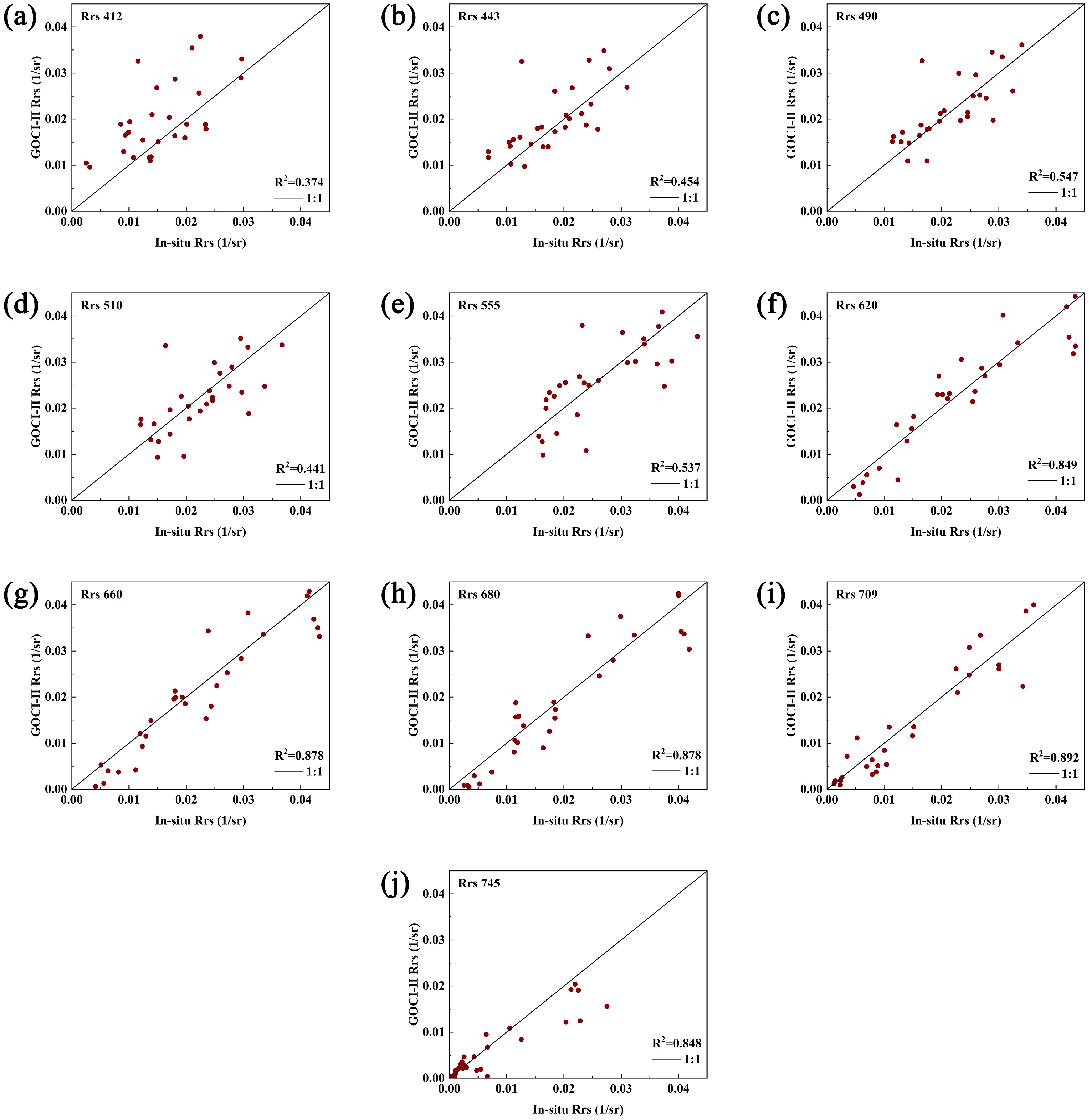
Figure 4. Comparison of the Rrs values derived from the GOCI-II data with the measured Rrs values. (a–j) compare GOCI-II data retrieved versus measured Rrs values at 412, 443, 490, 510, 555, 620, 660, 680, 709, and 745 nm, with the central diagonal indicating the 1:1 reference line.).

Table 2

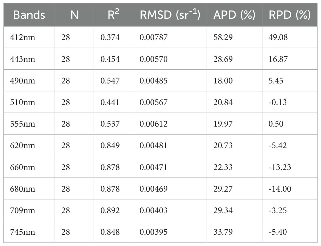
Table 2. Statistical results of the comparison between the Rrs values for each wavelength band obtained through the GOCI-II data and the measured Rrs values for each wavelength band.

3.2 Analysis of the spectral characteristics of different algal species

Through the algal cultivation experiments, spectral curves for typical dinoflagellates (K. mikimotoi) and diatoms (S. costatum) in the ECS were obtained during their bloom periods, as shown in Figure 5. The data indicated that the fluorescence peak of the algal spectrum changed at different growth and blooming stages. For example, the fluorescence peak of K. mikimotoi occurred at 688 nm from days 1 to 5 (Figure 6), and from days 6 to 11, it shifted to a range between 701 and 707 nm. For S. costatum, the fluorescence peak occurred at 688 nm from days 1 to 8 and gradually shifted to 701 nm from days 9 to 15. This is consistent with the findings of previous studies (O’Reilly et al., 1998), which showed that in different water bodies, the fluorescence peak wavelength shifts within the 680 to 710 nm range with increasing Chl a concentration.

Figure 5

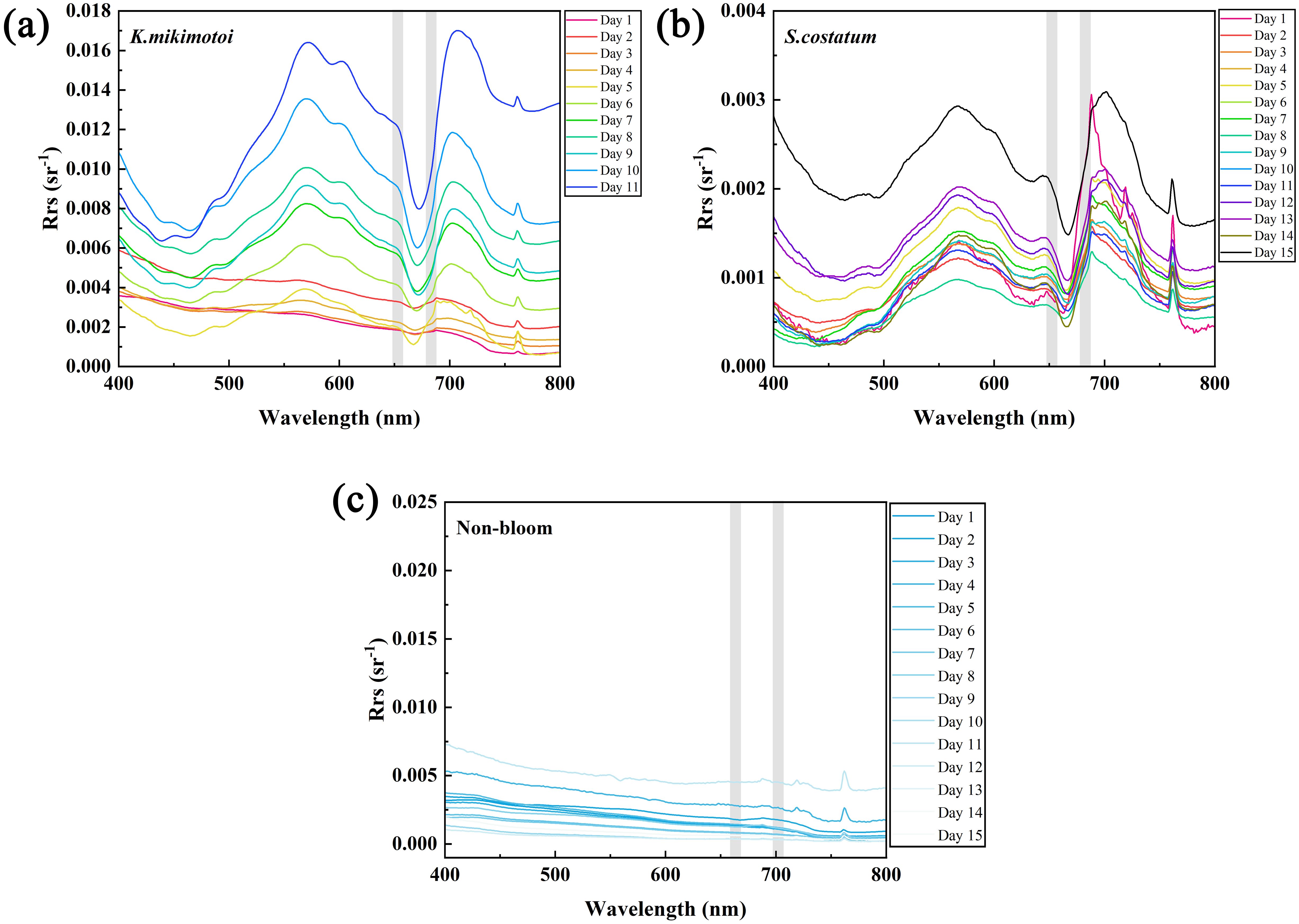
Figure 5. Spectral variations of K mikimotoi (a) and S. costatum (b) during bloom periods, along with the spectral results of the pure seawater control group (c) (the different curves show spectral results at different times. In the figure, the gray bar indicates the positions of the GOCI-II fluorescence bands at 680 and 709 nm. a: K mikimotoi; b: S. costatum).

Figure 6

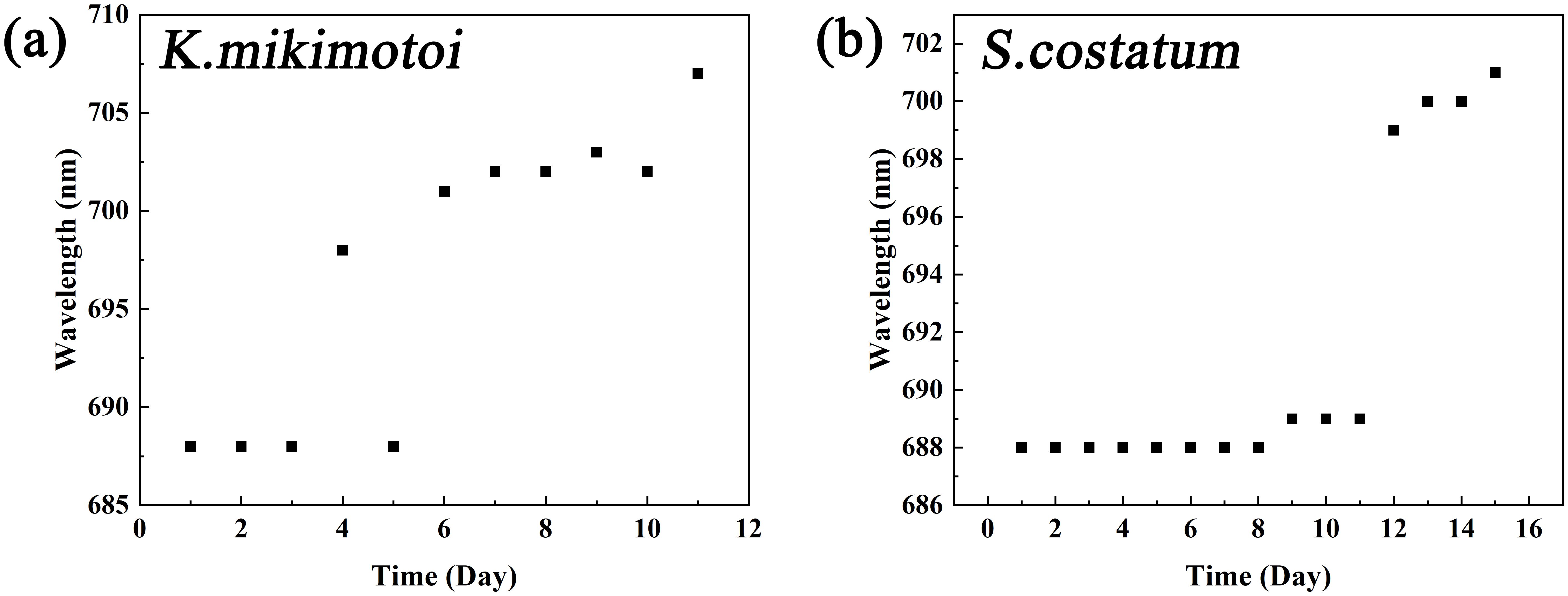
Figure 6. Changes in the algal cell fluorescence peak bands over time (a: K mikimotoi; b: S. costatum).

Previous algal bloom detection methods did not adequately account for the redshift in the fluorescence peak, leading to less accurate identification (Hu et al., 2005). The spectral curves of algal bloom water samples are influenced by chlorophyll fluorescence (compare with Figure 5), with significantly higher Rrs values at the fluorescence peak band (680 or 709 nm) than those at 660 nm, which is affected by chlorophyll absorption peaks and pure water absorption. Therefore, distinguishing between algal bloom and nonbloom waters can be based on the difference in the Rrs value between the fluorescence peak bands and the 660 nm band. The BIF can be calculated using Equations 10, 11.

$\begin{array}{ll}{\text{BI}}_{\text{F}}=\text{M}-\text{Rrs}660& (10)\end{array}$

$\begin{array}{ll}\text{M}=\text{max}(\text{Rrs}680,\text{Rrs}709)& (11)\end{array}$

Where BI_F is the fluorescence-based bloom index. In addition to using BI_F, Chl a was employed to assist in identifying algal bloom waters, thereby avoiding anomalies caused by elevated near-infrared bands due to high suspended particulate concentrations in water. Currently, there is no standard Chl a threshold for identifying algal bloom waters in the ECS. Shang et al. (2014) proposed a Chl a threshold of 5 µg/L, while other measurement-based studies revealed Chl a values during HABs ranging from 5.31 to 37.73 µg/L, with a median of 10.9 µg/L (Shen et al., 2019). In this study, the Chl a threshold was set to 4 µg/L, with the assumption that Chl a concentrations in algal bloom waters are greater than this value.

The corresponding fluorescence quantum yield was calculated on the basis of the experimentally measured spectral data. The fluorescence quantum yield was calculated via the method of Goodwin et al. as Equations 12, 13 (Goodwin, 2011):

$\begin{array}{ll}\text{φ}=0.37\frac{\text{FLH}}{{\text{Chla}}^{0.657}}& (12)\end{array}$

Formula 12 is derived from the following formula:

$\begin{array}{ll}\text{φ}=\frac{\text{FLH}}{\text{Chla} *\langle {\text{a}}_{\text{ph}}^{*}\rangle * \text{S}}& (13)\end{array}$

where $\langle {\text{a}}_{\text{ph}}^{*}\rangle$ is the spectral average of phytoplankton specific absorption coefficients and S is approximately 100 mWcm^-2μm^-1sr^-1m. The coefficients in the formula 12 are derived from Goodwin’s estimates of the spectral average of phytoplankton specific absorption coefficients ($\langle {\text{a}}_{\text{ph}}^{*}\rangle$) in the main photosynthetic absorption band (400–530 nm) and a minor adjustment to FLH in formula 13.

The FLH can be calculated using Equation 14 (Gower and Borstad, 2004):

$\begin{array}{ll}\text{FLH}={\text{nLw}}_F-[{\text{nLw}}_R+\frac{{\text{λ}}_R-{\text{λ}}_F}{{\text{λ}}_R-{\text{λ}}_L}*({\text{nLw}}_L-{\text{nLw}}_R)]& (14)\end{array}$

where ${\text{nLw}}_{\text{F}}$ denotes the nLw value of the fluorescence peak band, ${\text{nLw}}_{\text{R}}$ denotes the nLw value of the right baseline band, and ${\text{nLw}}_{\text{L}}$ denotes the nLw value of the left baseline band. Moreover, λ_F, λ_L and λ_R are the central wavelengths of the fluorescence band and the two baseline bands, respectively.

Figure 7 shows the variation in the fluorescence quantum yield of the two types of algae throughout their growth phase, until the outbreak of the algal bloom, and into the initial stages of their decline. Although the fluorescence quantum yield fluctuated with algae growth—for example, the φ value of S. costatum ranged from 0.01 to 0.016 during the bloom period, while the φ value of K. mikimotoi ranged from 0.003 to 0.007 during the growth period—the differences in the fluorescence quantum yield between the different algal species were significant. Therefore, this characteristic could be used for algal species classification.

Figure 7

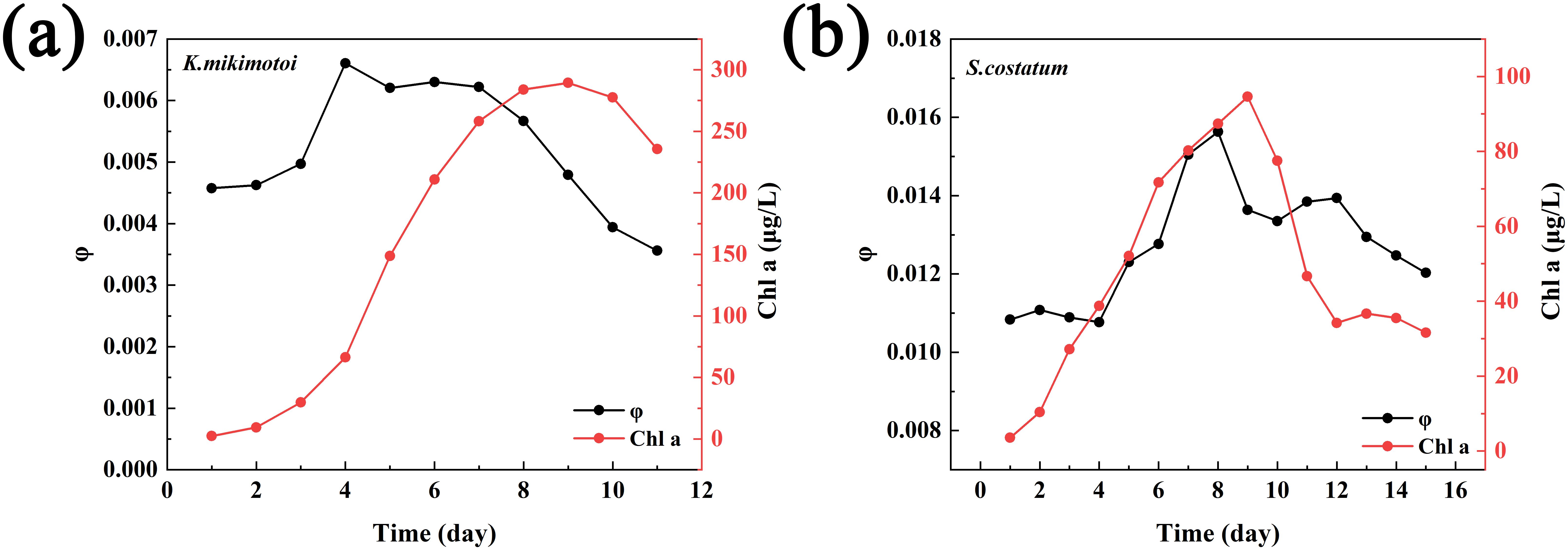
Figure 7. Variations in φ and Chl a during the bloom periods of the two types of phytoplankton (a: K mikimotoi; b: S. costatum).

On the basis of the spectral characteristics of bloom waters and the differences in the phytoplankton fluorescence quantum yield obtained via the algae cultivation experiments, the bloom water identification and dominant phytoplankton classification process established in this study is shown in Figure 8. First, on the basis of the GOCI-II band settings, the band with higher Rrs values at 709 or 680 nm is selected as the fluorescence peak band, and the difference from the fluorescence left baseline band at 660 nm is calculated. Additionally, the chlorophyll concentration is used as an auxiliary criterion to identify bloom waters. Then, with the use of the fluorescence quantum yield threshold, the dominant phytoplankton species in bloom waters can be classified.

Figure 8

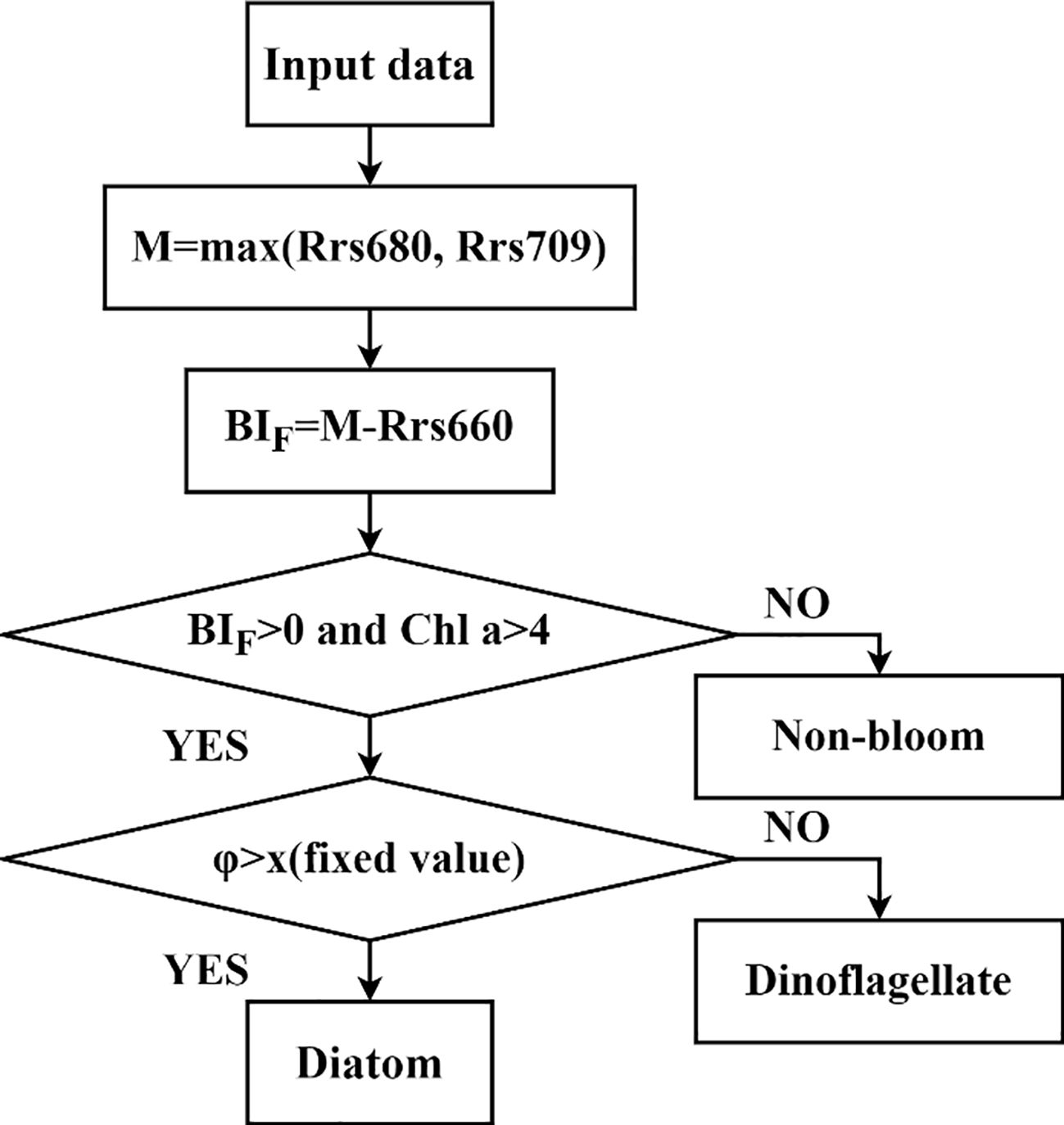
Figure 8. Flowchart of the φ method for distinguishing between dinoflagellate and diatom blooms.

3.3 Application of the fluorescence-based bloom index for algal bloom water identification

In this study, five dinoflagellate bloom events and two diatom bloom events from 2021 to 2023 were selected to validate the applicability of the proposed algal bloom water identification method. Figure 9 shows the application results of different algal bloom water identification algorithms for diatom bloom events in September 2021 and July 2022. The data presented in Figures 9 were derived from satellite observations acquired around local noon (between 11:30 and 13:30 local time). Although geostationary ocean color satellites can perform multiple observations throughout the day, the data acquired at noon generally exhibit significantly higher accuracy compared to other time periods. Therefore, this study employed the noon-time data for analysis. The black boxes in the figure highlight the areas reported for HABs in the Bulletin of China Marine Disasters. The BI_F method, which incorporates the Chl a concentration and accounts for the redshift in the fluorescence peak, clearly provided significantly better bloom water identification results than those of the other three methods. The SS and LHR methods were more accurate in identifying water bodies with large-scale blooms, where the redshift in the fluorescence peak was greater. However, they failed to accurately identify the two diatom blooms. With the use of the RI method, the diatom blooms in September 2021 were successfully detected, but clean ocean waters were incorrectly identified as bloom waters over a large area.

Figure 9

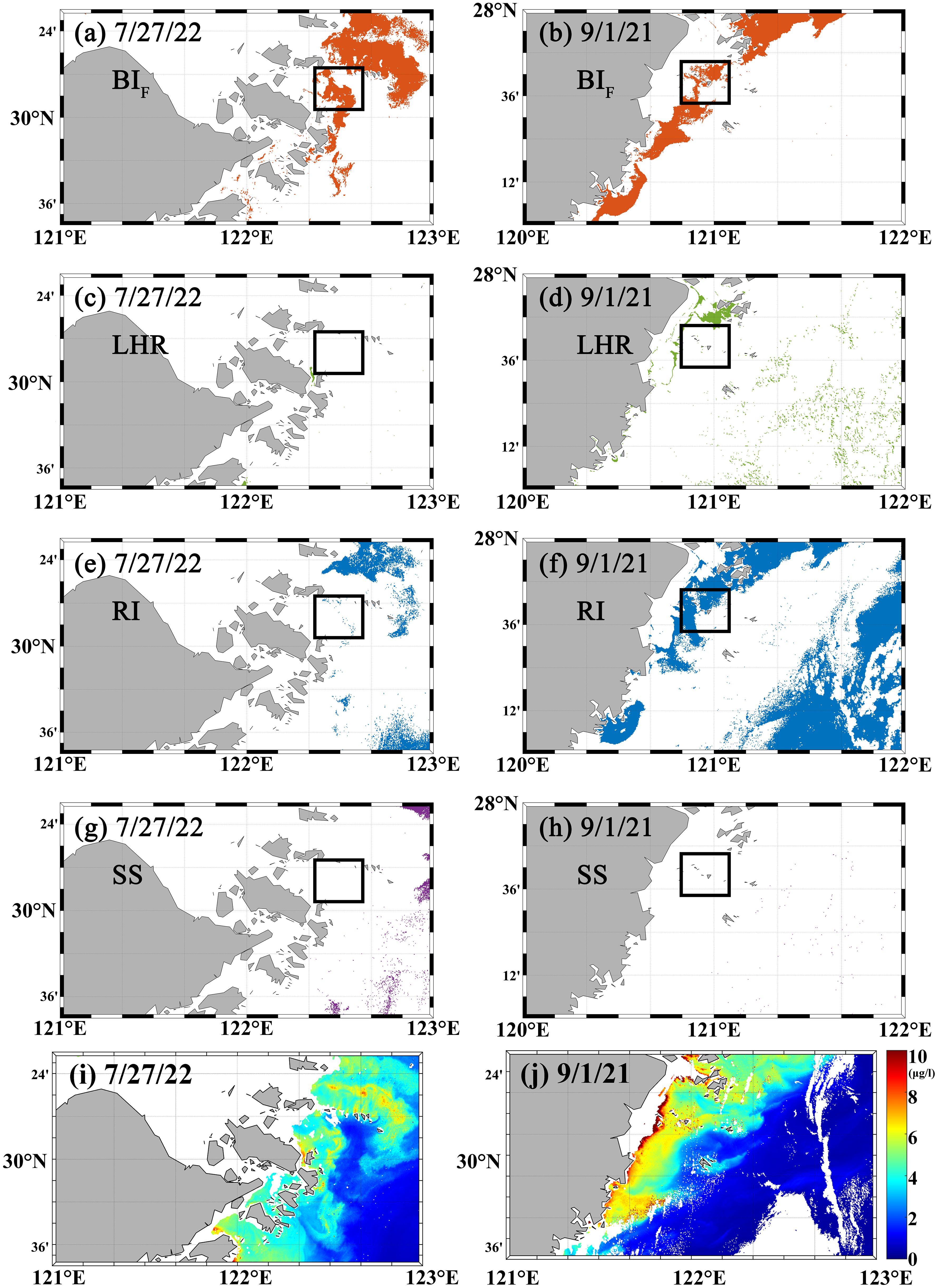
Figure 9. Results of the different methods for identifying diatom blooms. (White areas indicate regions without detected blooms; black boxes show HAB locations reported in the Bulletin of China Marine Disasters.) (a, b) show BI_F results on July 27, 2022, and September 1, 2021. (c–h) show corresponding results from the LHR, RI, and SS methods. (i, j) show he corresponding chl a concentrations.

Similar to Figure 9, Figure 10 shows the application results of the different algal bloom water identification algorithms for the five dinoflagellate bloom events. All five dinoflagellate bloom events were detected via the RI and BI_F methods, whereas four out of the five bloom events could be identified via the LHR method, and none of the blooms could be detected via the SS method. Overall, the BI_F method was the most accurate for identifying bloom waters. The other three methods exhibited instances of misidentification. For example, the RI method may be affected by the absorption of CDOM and suspended particulate matter (SPM), leading to high RI values in coastal waters with high suspension rates, which can cause misidentification in coastal areas. In the LHR method, oceanic waters could be mistakenly identified as bloom waters.

Figure 10

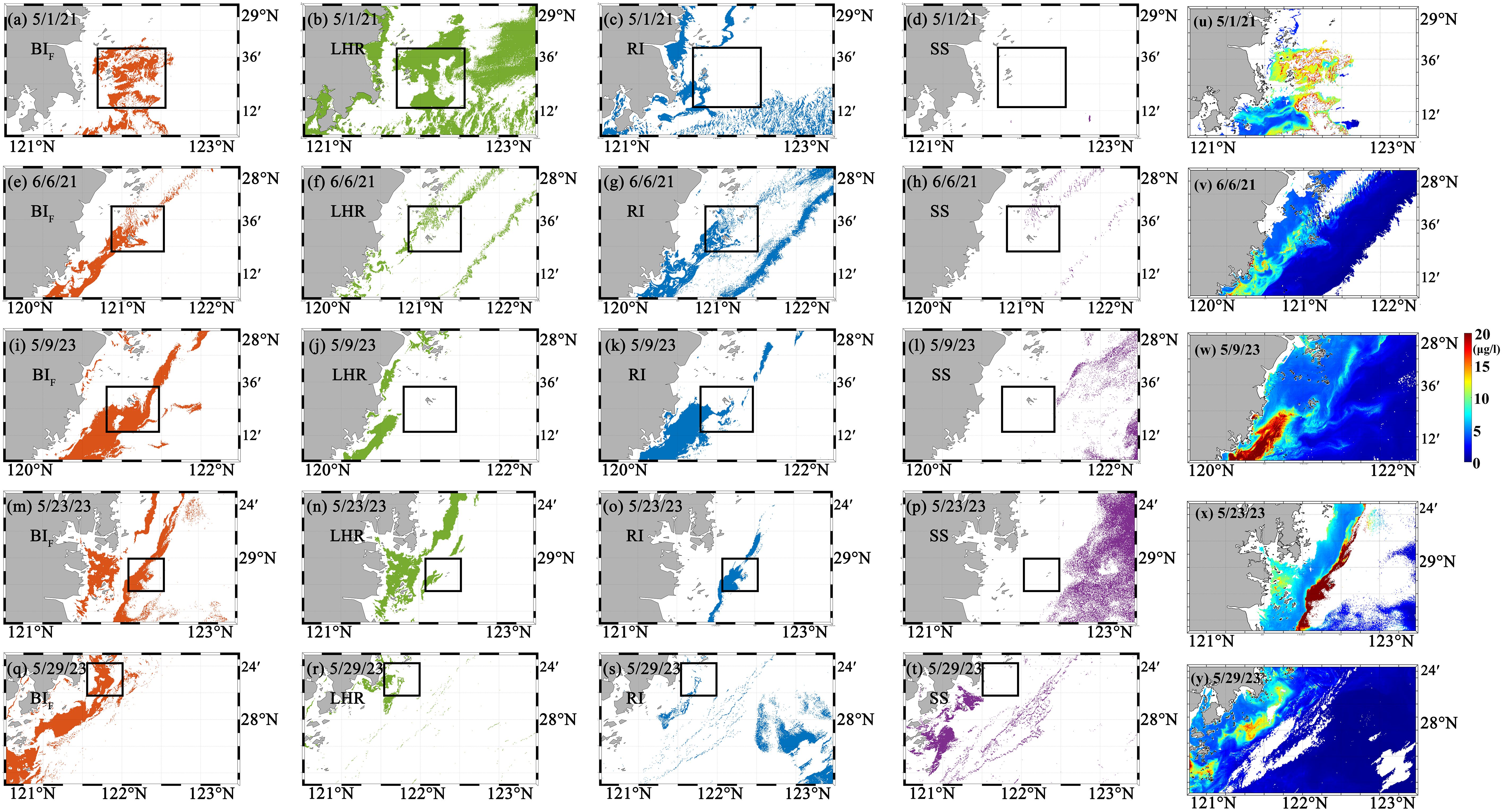
Figure 10. Results of the different methods for identifying dinoflagellate blooms. (White areas indicate regions without detected blooms; black boxes show HAB locations reported in the Bulletin of China Marine Disasters.) (a–d) show the results of the BIF, LHR, RI, and SS algorithms on May 1, 2021. (e–t) present the corresponding algorithm results on June 6, 2021, May 9, 2023, May 23, 2023, and May 29, 2023. (u–y) show the corresponding chl a concentrations.

3.4 Differentiation between diatom and dinoflagellate blooms

On the basis of the differences in the fluorescence quantum yield among algal species, bloom waters can be classified according to the dominant algal species. Figure 11a presents a scatter plot of the GOCI-II φ and BI_F, plotted using in-situ data from the 2019 cruise and seven algal bloom events between 2021 and 2023 (The locations of the algal blooms are shown in Figure 2). While different algal species exhibit different ranges of φ due to the influence of suspended particles or CDOM in water, there is a significant difference in the φ between species. During bloom events, the φ of diatoms is generally greater than 0.014, whereas that of dinoflagellates is generally less than 0.014. Therefore, the above φ threshold can be used to effectively distinguish between different dominant algal species in blooms. In contrast, Figure 11b illustrates the differentiation of diatom and dinoflagellate blooms using the Bloom Index (BI), which is based on the blue/green spectral slope. The BI is defined as the ratio of the spectral slopes of Rrs measured in two spectral ranges (443–488 nm and 531–555 nm). A BI value in the range of 0.0 < BI ≤ 0.3 indicates a dinoflagellate bloom, while a BI value in the range of 0.3 < BI ≤ 1.0 indicates a diatom bloom. As shown in the figure, while the BI algorithm can generally identify diatom blooms across different times and regions, it exhibits limited accuracy in distinguishing dinoflagellate blooms. Specifically, the BI algorithm fails to sufficiently and correctly differentiate dinoflagellate blooms in many cases. This likely occurs because the slope calculated via the 510 nm band of GOCI-II rather than via the 531 nm band of MODIS is slightly underestimated, thereby not reflecting the spectral characteristics of different algal species.

Figure 11

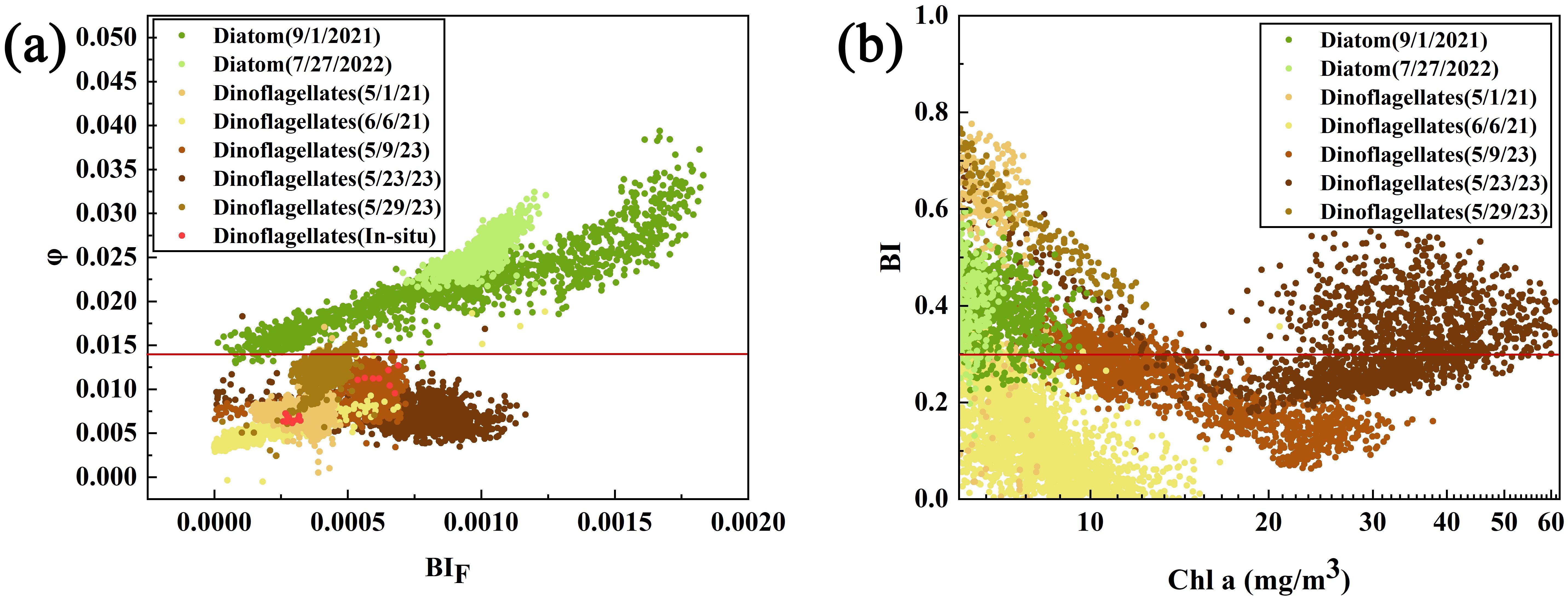
Figure 11. Classification results for the dinoflagellate and diatom bloom regions via the φ and BI methods. (a) Classification results for the dinoflagellate and diatom bloom regions via the φ methods; (b) Classification results for the dinoflagellate and diatom bloom regions via the BI methods. logarithmic scaling (log10) on x-axis resolves Chl a concentrations across orders of magnitude).

3.5 Variation in the dominant algal species

By using the algal bloom detection and dominant species classification algorithms developed in this study, it is possible to effectively observe variations in coastal algal bloom waters. Figure 12 shows images of the key stages in the algae species transition during an algal bloom event on the eastern side of Sanmen Bay, ECS, from September 1, 2021, to October 3, 2021, the research time is 3:15 PM local time. According to information from the China Marine Disaster Bulletin, this region experienced consecutive algal bloom events, with a transition from diatom blooms to dinoflagellate blooms.

Figure 12

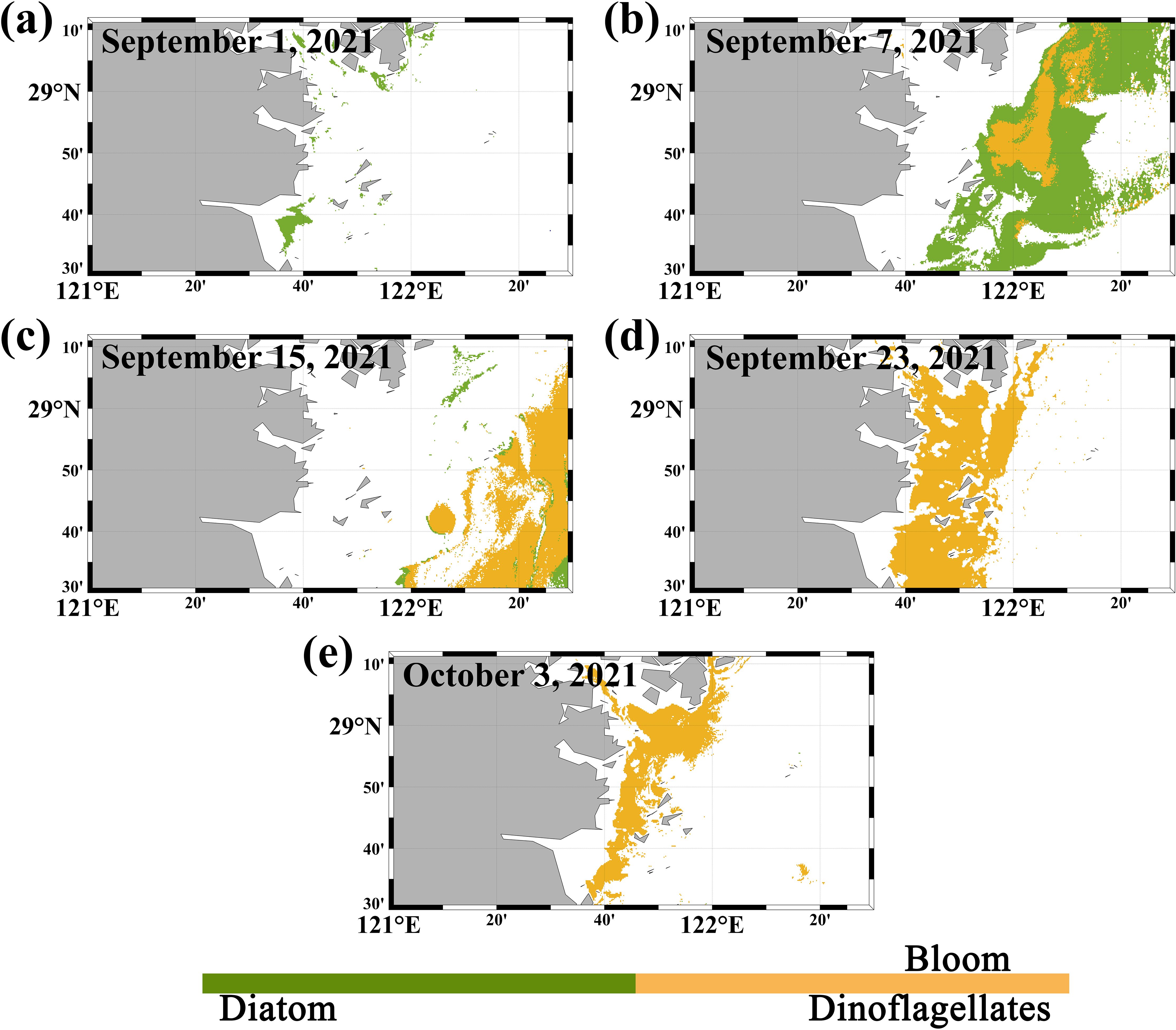
Figure 12. Development process of dinoflagellate and diatom blooms identified via the new method proposed in this study. (The white areas include regions partially covered by clouds as well as areas determined not to be algal blooms based on the BI_F algorithm. (a–e) represent the results from September 1, September 7, September 15, September 23, and October 3, 2021, respectively.).

The algorithm developed in this study clearly revealed the transition process from diatom blooms to dinoflagellate blooms. Due to the outbreak of diatom blooms on September 1, 2021, the water surface was predominantly characterized by diatom blooms on that date, Although there were no cloud cover in the satellite images, the area covered by diatom blooms was relatively small. After September 1, 2021, the area of diatom blooms gradually increased. From the results on September 7, 2021, it can be observed that both diatom and dinoflagellate blooms were present at that time, with the area of diatom blooms being larger, after September 23, 2021, the algal blooms in the water completely transitioned to dinoflagellate blooms. The occurrence of this phenomenon may be attributed to Sanmen Bay’s location along the eastern coast of Zhejiang, where the bay experiences relatively mild winds and waves, and has broad intertidal zones. This makes it an important fishing resource production base in Zhejiang Province, resulting in high nutrient levels in the seawater, which can easily lead to algal blooms. The water body has shifted from diatom-dominated blooms to dinoflagellate-dominated blooms primarily due to a significant decrease in water temperature in Sanmen Bay from early September to early October 2021 (Kong et al., 2022). High temperatures are more favorable for diatom growth, and the reduction in temperature can inhibit their growth.

While our results are preliminary, they demonstrate significant potential for future research on the spatiotemporal distribution patterns and dynamics of diatom and dinoflagellate blooms in coastal marine environments. Such studies could help explain the impacts of climate change and human activities on future distribution patterns.

4 Discussion

Based on experimental and satellite data analysis, it has been found that φ can distinguish algal bloom waters or different dominant algal species. However, natural water constituents, such as CDOM and suspended sediments, may affect the φ value. Therefore, this study utilized the radiative transfer model software Hydrolight 5.0, developed by Sequoia Scientific, Inc., USA, to simulate the impact of CDOM and total suspended matter (TSM) on φ. The study predefined three specific water body types: clear ocean waters, continental shelf waters, and nearshore waters. Table 3 shows the specific concentrations of 3 key water color parameters in these 3 water bodies.

Table 3

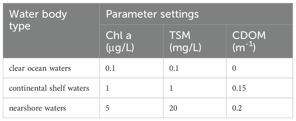
Table 3. The specific concentrations of the 3 key water color parameters in these 3 water bodies.

The basic settings for the Hydrolight simulations were as follows: since the stationary satellite GOCI-II cannot retrieve water color parameters from deeper underwater locations, the vertical distribution values for Chl a concentration, CDOM concentration, and TSM concentration were set as constants independent of depth (Chai et al., 2020). The specific absorption and scattering coefficients for suspended sediments were selected based on data related to yellow clay (Haltrin, 1999). The absorption and scattering characteristics of water bodies were chosen based on the results of Pope et al (Pope and Fry, 1997; Haltrin, 1999), and the scattering properties of particles were defined using the Petzold phase function (Wei et al., 2014). Bioluminescence phenomena were not considered in this experiment. The wavelength range selected for the simulations began at 397.5 nm, with intervals of 1 nm or 5 nm, up to 800 nm. The wind speed at the air-water interface was set to 0.5 m/s, and the weather model was based on the semi-empirical RADTRAN model, with cloud cover set to 0%. The bottom boundary was defined as infinite depth.

When setting the step sizes for the variation of the 3 key water color parameters, specific parameters are shown in Table 4, including Chl a concentration, TSM concentration, CDOM absorption coefficient at 443 nm (aCDOM(443 nm)), and solar zenith angle, with fixed step sizes. In low-turbidity waters, even slight changes in water color components can lead to significant variations in satellite spectral signals, so smaller simulation step sizes were used. In high-turbidity waters, satellite signals may become oversaturated, leading to smaller relative changes, and thus larger simulation step sizes were applied.

Table 4

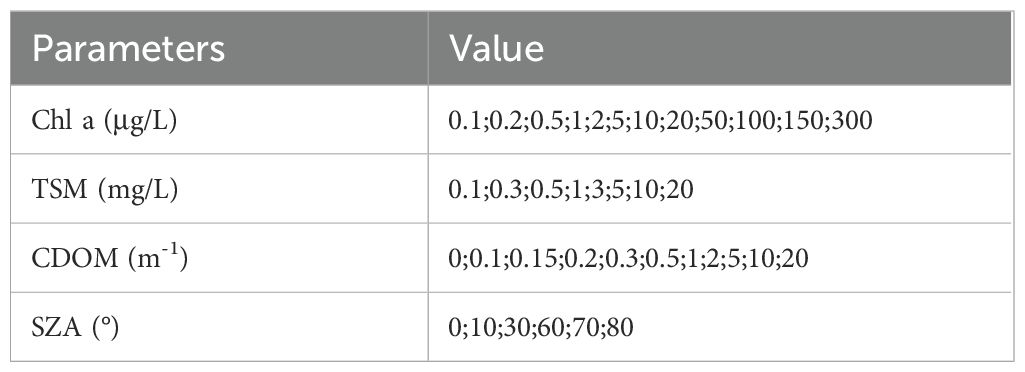
Table 4. Parameters used for dataset simulation with Hydrolight.

Figure 13a shows the impact of CDOM variations on φ in different water bodies. The sensitivity analysis of the fluorescence peak to CDOM variations indicates that in all three water bodies, changes in CDOM concentration have little to no effect on the fluorescence peak wavelength and fluorescence peak value. Therefore, the fluorescence peak remains present across the entire CDOM concentration range from 0.1 m^-¹ to 20 m^-¹, allowing for the calculation of FLH values. As shown in the figure, φ decreases with increasing CDOM concentration in all water bodies. This is because the absorption peak of CDOM lies within the absorption wavelength range of Chl a, meaning it competes with Chl a molecules for light absorption. As CDOM concentration increases, more light energy is absorbed by CDOM, reducing the available light energy to excite Chl a molecules, which results in a decrease in φ. However, this effect is limited, and thus φ shows minimal variation with changes in CDOM concentration across different water bodies.

Figure 13

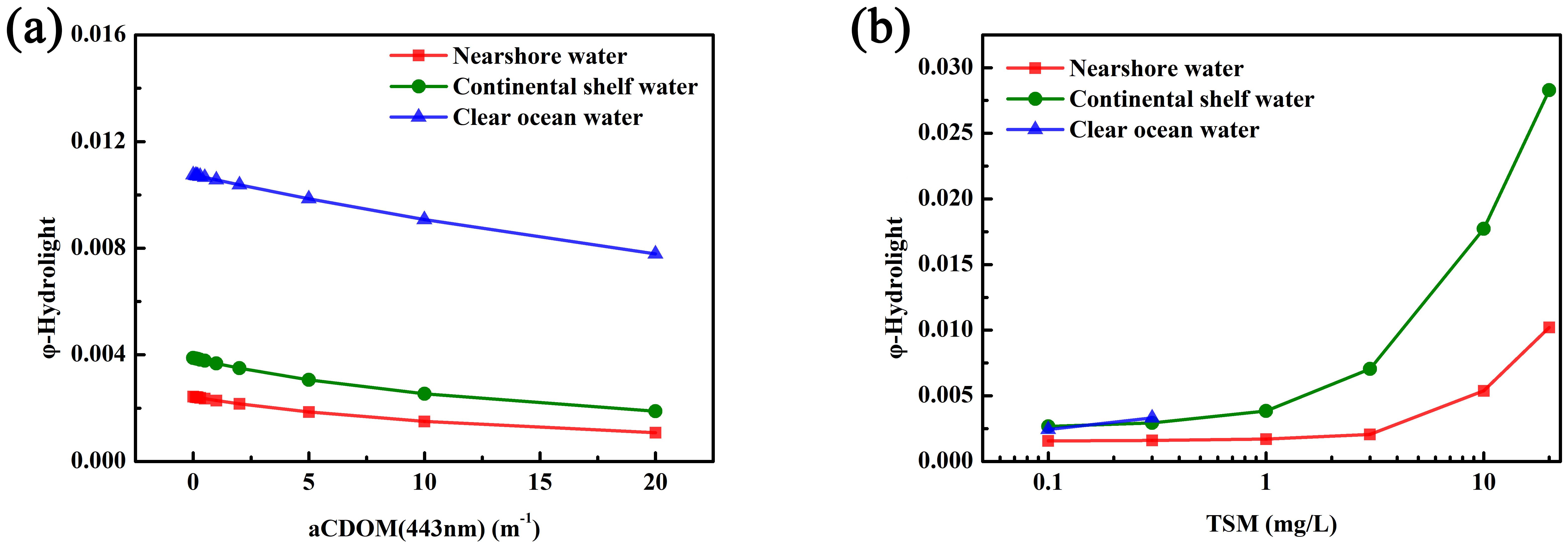
Figure 13. The Impact of Different CDOM and TSM Concentration Variations on φ Simulation Results in Different Water Bodies. (a) The impact of CDOM variations on φ in different water bodies; (b) The impact of TSM variations on φ in different water bodies).

Figure 13b shows the impact of TSM variations on φ in different water bodies. As observed in the figure, the amplitude of φ changes with TSM decreases from clear ocean waters to nearshore waters. When TSM is 0.1 mg/L, φ in all three water bodies is mainly influenced by Chl a concentration, with the highest Chl a concentration found in nearshore waters, resulting in the lowest φ. As TSM concentration increases in different water bodies, φ also increases. This is because, as TSM concentration rises, scattering effects are enhanced, which raises the overall fluorescence peak, thereby increasing the calculated φ.

The CDOM concentration in the nearshore waters of the East China Sea did not reach the elevated levels predicted by the dataset, resulting in a minimal impact on φ. However, variations in TSM concentrations lead to corresponding changes in φ. Consequently, the φ value of 0.014, which serves as the threshold for distinguishing between dinoflagellate and diatom blooms in this study, is only relevant for differentiating blooms in the East China Sea’s nearshore waters. Its applicability to other aquatic environments still requires further validation.

5 Conclusion

Dinoflagellate and diatom blooms are among the most common marine hazards in the YRE and adjacent ECS areas. The use of Chl a to identify HABs poses significant challenges with respect to misclassification. The GOCI-II fluorescence band Rrs products are relatively close to the measured values, which is advantageous for bloom detection and classification. Therefore, leveraging the GOCI-II fluorescence bands, the differences in φ between dinoflagellate and diatom blooms during their growth phases in the ECS were quantified on the basis of algal culture experiments, and a bloom detection and classification method suitable for GOCI-II data was developed.

On the basis of the water body spectral characteristics obtained from the algal culture experiments, a bloom detection method was established on the basis of the difference in the Rrs value between the fluorescence peak band and the left baseline band. A bloom classification method was subsequently developed using φ, with a threshold of 0.014, to distinguish between dinoflagellate and diatom blooms. The experiments and methods in this study were conducted in waters with relatively high Chl a concentrations, and the algorithm does not address scenarios where the Chl a concentration is below 4 μg/L. The application of the developed bloom detection and classification methods to GOCI-II imagery could allow accurate observation of bloom spatial distributions and temporal changes. It could also facilitate the precise classification of dinoflagellate and diatom blooms in the ECS, which could help coastal managers better mitigate the harmful impacts of blooms in the region.

Data availability statement

The original contributions presented in the study are included in the article/supplementary material. Further inquiries can be directed to the corresponding author.

Author contributions

MZ: Writing – original draft, Conceptualization, Formal analysis, Funding acquisition, Investigation, Methodology, Writing – review & editing. HL: Writing – review & editing. XZ: Conceptualization, Writing – review & editing. XD: Investigation, Software, Writing – review & editing. FG: Data curation, Methodology, Supervision, Writing – review & editing.

Funding

The author(s) declare that financial support was received for the research and/or publication of this article. This research was funded by the National Key Research and Development Program of China (Grant #2023YFC3108101), the National Natural Science Foundation of China (Grant #U23A2037, #42206183), the “Pioneer” R&D Program of Zhejiang (2023C03011), the Zhejiang Provincial Natural Science Foundation of China (Grant #LDT23D06021D06), and the project of the Donghai Laboratory (#L24QH013, #DH-2023QH0002).

Acknowledgments

We would like to thank the staff of the satellite ground station, satellite data processing and sharing center, and marine satellite data online analysis platform of the State Key Laboratory of Satellite Ocean Environment Dynamics, Second Institute of Oceanography, Ministry of Natural Resources (SOED/SIO/MNR) for their help with data processing.

Conflict of interest

The authors declare that the research was conducted in the absence of any commercial or financial relationships that could be construed as a potential conflict of interest.

The reviewer PC declared a shared affiliation with the authors XZ and FG.

Generative AI statement

The author(s) declare that no Generative AI was used in the creation of this manuscript.

Publisher’s note

All claims expressed in this article are solely those of the authors and do not necessarily represent those of their affiliated organizations, or those of the publisher, the editors and the reviewers. Any product that may be evaluated in this article, or claim that may be made by its manufacturer, is not guaranteed or endorsed by the publisher.

References

Ahn J. H., Park Y. J., Kim W., and Lee B. (2016). Simple aerosol correction technique based on the spectral relationships of the aerosol multiple-scattering reflectances for atmospheric correction over the oceans. Optics express 24, 29659–29669. doi: 10.1364/OE.24.029659

PubMed Abstract | Crossref Full Text | Google Scholar

Anderson C. R., Berdalet E., Kudela R. M., Cusack C. K., Silke J., O’Rourke E., et al. (2019). Scaling up from regional case studies to a global harmful algal bloom observing system. Front. Mar. Sci. 6. doi: 10.3389/fmars.2019.00250

Crossref Full Text | Google Scholar

Anderson D. M., Cembella A. D., and Hallegraeff G. M. (2012). Progress in understanding harmful algal blooms: paradigm shifts and new technologies for research, monitoring, and management. Annu. Rev. Mar. Sci. 4, 143–176. doi: 10.1146/annurev-marine-120308-081121

PubMed Abstract | Crossref Full Text | Google Scholar

Bannister T. T. and Weidemann A. D. (1984). The maximum quantum yield of phylopiankton photosynthesis in situ. J. plankton Res. 6, 275–294. doi: 10.1093/plankt/6.2.275

Crossref Full Text | Google Scholar

Behrenfeld M. J., Westberry T. K., Boss E., O’Malley R. T., Siegel D. A., Wiggert J. D., et al. (2009). Satellite-detected fluorescence reveals global physiology of ocean phytoplankton. Biogeosciences 6, 779–794. doi: 10.5194/bg-6-779-2009

Crossref Full Text | Google Scholar

Chai F., Johnson K. S., Claustre H., Xing X., Wang Y., Boss E., et al. (2020). Monitoring ocean biogeochemistry with autonomous platforms. Nat. Rev. Earth Environ. 1, 315–326. doi: 10.1038/s43017-020-0053-y

Crossref Full Text | Google Scholar

Chen B., Jin Y., and Brown P. (2019). An enhanced bloom index for quantifying floral phenology using multi-scale remote sensing observations. ISPRS J. Photogrammetry Remote Sens. 156, 108–120. doi: 10.1016/j.isprsjprs.2019.08.006

Crossref Full Text | Google Scholar

Domrös M. and Peng G. (2012). The climate of China. Springer science and business media. Berlin and Heidelberg, Germany: Springer.

Google Scholar

Falkowski P. G. and Kolber Z. (1995). Variations in chlorophyll fluorescence yields in phytoplankton in the world oceans. Funct. Plant Biol. 22, 341–355. doi: 10.1071/PP9950341

Crossref Full Text | Google Scholar

Goodwin D. (2011). Satellite-derived fluorescence quantum yields as indicators of phytoplankton photophysiology (University of New Hampshire).

Google Scholar

Gower J. F. R. and Borstad G. A. (2004). On the potential of MODIS and MERIS for imaging chlorophyll fluorescence from space. Int. J. Remote Sens. 25, 1459–1464. doi: 10.1080/01431160310001592445

Crossref Full Text | Google Scholar

Guan W., Bao M., Lou X., Zhou Z., and Yin K. (2022). Monitoring, modeling and projection of harmful algal blooms in China. Harmful Algae 111, 102164. doi: 10.1016/j.hal.2021.102164

PubMed Abstract | Crossref Full Text | Google Scholar

Guo S., Feng Y., Wang L., Dai M., Liu Z., Bai Y., et al. (2014). Seasonal variation in the phytoplankton community of a continental-shelf sea: the East China Sea. Mar. Ecol. Prog. Ser. 516, 103–126. doi: 10.3354/meps10952

Crossref Full Text | Google Scholar

Haltrin V. I. (1999). Chlorophyll-based model of seawater optical properties. Appl. Optics 38, 6826–6832. doi: 10.1364/AO.38.006826

PubMed Abstract | Crossref Full Text | Google Scholar

He X., Bai Y., Pan D., Huang N., Dong X., Chen J., et al. (2013). Using geostationary satellite ocean color data to map the diurnal dynamics of suspended particulate matter in coastal waters. Remote Sens. Environ. 133, 225–239. doi: 10.1016/j.rse.2013.01.023

Crossref Full Text | Google Scholar

Hu C. and Feng L. (2017). Modified MODIS fluorescence line height data product to improve image interpretation for red tide monitoring in the eastern Gulf of Mexico. J. Appl. Remote Sens. 11, 012003–012003. doi: 10.1117/1.JRS.11.012003

Crossref Full Text | Google Scholar

Hu C., Muller-Karger F. E., Taylor C. J., Carder K. L., Kelble C., Johns E., et al. (2005). Red tide detection and tracing using MODIS fluorescence data: A regional example in SW Florida coastal waters. Remote Sens. Environ. 97, 311–321. doi: 10.1016/j.rse.2005.05.013

Crossref Full Text | Google Scholar

Kong Y. F., Yin C. J., Wang L. L., Liu Y., Lin L., and Kang B. (2022). Ecosystem structure and function of Sanmen Bay based on Ecopath model. Ying Yong Sheng tai xue bao= J. Appl. Ecol. 33, 829–836. doi: 10.13287/j.1001-9332.202202.034

PubMed Abstract | Crossref Full Text | Google Scholar

Lamquin N., Mazeran C., Doxaran D., Ryu J. H., and Park Y. J. (2012). Assessment of GOCI radiometric products using MERIS, MODIS and field measurements. Ocean Sci. J. 47, 287–311. doi: 10.1007/s12601-012-0029-z

Crossref Full Text | Google Scholar

Li J., Glibert P. M., and Zhou M. (2010). Temporal and spatial variability in nitrogen uptake kinetics during harmful dinoflagellate blooms in the East China Sea. Harmful Algae 9, 531–539. doi: 10.1016/j.hal.2010.03.007

Crossref Full Text | Google Scholar

Li H., He X., Bai Y., et al. (2020). Atmospheric correction of geostationary satellite ocean color data under high solar zenith angles in open oceans. Remote Sens. Environ. 249, 112022. doi: 10.1016/j.rse.2020.112022

Crossref Full Text | Google Scholar

Lichtenthaler H. K. and Rinderle U. (1988). The role of chlorophyll fluorescence in the detection of stress conditions in plants. CRC Crit. Rev. Analytical Chem. 19, S29–S85. doi: 10.1080/15476510.1988.10401466

Crossref Full Text | Google Scholar

Lou X. and Hu C. (2014). Diurnal changes of a harmful algal bloom in the East China Sea: Observations from GOCI. Remote Sens. Environ. 140, 562–572. doi: 10.1016/j.rse.2013.09.031

Crossref Full Text | Google Scholar

Maxwell K. and Johnson G. N. (2000). Chlorophyll fluorescence—a practical guide. J. Exp. Bot. 51, 659–668. doi: 10.1093/jexbot/51.345.659

Crossref Full Text | Google Scholar

Mueller J. L., Pietras C., Hooker S. B., Austin R. W., Miller M., Knobelspiesse K. D., et al. (2003). “Ocean optics protocols for satellite ocean color sensor validation, revision 4,” in Volume II: instrument specifications, characterization and calibration. NASA Goddard Space Flight Center, Greenbelt, Maryland, USA.

Google Scholar

Murchie E. H. and Lawson T. (2013). Chlorophyll fluorescence analysis: a guide to good practice and understanding some new applications. J. Exp. Bot. 64, 3983–3998. doi: 10.1093/jxb/ert208

PubMed Abstract | Crossref Full Text | Google Scholar

O’Reilly J. E., Maritorena S., Mitchell B. G., Siegel D. A., Carder K. L., Garver S. A., et al. (1998). Ocean color chlorophyll algorithms for SeaWiFS. J. Geophysical Research: Oceans 103, 24937–24953. doi: 10.1029/98JC02160

Crossref Full Text | Google Scholar

Orlova T. Y., Aleksanin A. I., Lepskaya E. V., Efimova K. V., Selina M. S., Morozova T. V., et al. (2022). A massive bloom of Karenia species (Dinophyceae) off the Kamchatka coast, Russia, in the fall of 2020. Harmful Algae 120, 102337. doi: 10.1016/j.hal.2022.102337

PubMed Abstract | Crossref Full Text | Google Scholar

Peng Y., Zhang W., Yang X., Zhang Z., Zhu G., and Zhou S. (2024). Current status and prospects of algal bloom early warning technologies: A Review. J. Environ. Manage. 349, 119510. doi: 10.1016/j.jenvman.2023.119510

PubMed Abstract | Crossref Full Text | Google Scholar

Pope R. M. and Fry E. S. (1997). Absorption spectrum (380–700 nm) of pure water. II. Integrating cavity measurements. Appl. optics 36, 8710–8723. doi: 10.1364/AO.36.008710

PubMed Abstract | Crossref Full Text | Google Scholar

Ralph P. J., Hill R., Doblin M. A., and Davy S. K. (2015). Theory and application of pulse amplitude modulated chlorophyll fluorometry in coral health assessment. Dis. coral, 506–523. doi: 10.1002/9781118828502.ch38

Crossref Full Text | Google Scholar

Sanseverino I., Conduto D., Pozzoli L., Dobricic S., and Lettieri T. (2016). Algal bloom and its economic impact. Eur. Commission Joint Res. Centre Institute Environ. Sustainability 51, 1–52. doi: 10.2788/660478

Crossref Full Text | Google Scholar

Shang S. L., Dong Q., Hu C. M., Lin G., Li Y. H., and Shang S. P. (2014). On the consistency of MODIS chlorophyll a products in the northern South China Sea. Biogeosciences 11, 269–280. doi: 10.5194/bg-11-269-2014

Crossref Full Text | Google Scholar

Shang S., Wu J., Huang B., Lin G., Lee Z., Liu J., et al. (2014). A new approach to discriminate dinoflagellate from diatom blooms from space in the East China Sea. J. Geophysical Research: Oceans 119, 4653–4668. doi: 10.1002/2014JC009876

Crossref Full Text | Google Scholar

Shen F., Tang R., Sun X., and Liu D. (2019). Simple methods for satellite identification of algal blooms and species using 10-year time series data from the East China Sea. Remote Sens. Environ. 235, 111484. doi: 10.1016/j.rse.2019.111484

Crossref Full Text | Google Scholar

Siswanto E., Ishizaka J., Tripathy S. C., and Miyamura K. (2013). Detection of harmful algal blooms of Karenia mikimotoi using MODIS measurements: A case study of Seto-Inland Sea, Japan. Remote Sens. Environ. 129, 185–196. doi: 10.1016/j.rse.2012.11.003

Crossref Full Text | Google Scholar

Tang D., Di B., Wei G., Ni I. H., Oh I. S., and Wang S. (2006). Spatial, seasonal and species variations of harmful algal blooms in the South Yellow Sea and East China Sea. Hydrobiologia 568, 245–253. doi: 10.1007/s10750-006-0108-1

Crossref Full Text | Google Scholar

Tao B., Mao Z., Lei H., Pan D., Shen Y., Bai Y., et al. (2015). A novel method for discriminating Prorocentrum donghaiense from diatom blooms in the East China Sea using MODIS measurements. Remote Sens. Environ. 158, 267–280. doi: 10.1016/j.rse.2014.11.004

Crossref Full Text | Google Scholar

Tao B., Mao Z., Wang D., Lu J., and Huang H. (2011). “The use of MERIS fluorescence bands for red tides monitoring in the East China Sea,” in Remote sensing of the ocean, sea ice, coastal waters, and large water regions, (439–446). SPIE – International Society for Optics and Photonics, Bellingham, Washington, USA. doi: 10.1117/12.898056

Crossref Full Text | Google Scholar

Wang J. and Wu J. (2009). Occurrence and potential risks of harmful algal blooms in the East China Sea. Sci. Total Environ. 407, 4012–4021. doi: 10.1016/j.scitotenv.2009.02.040

PubMed Abstract | Crossref Full Text | Google Scholar

Wei J., Lee Z., Pahlevan N., and Lewis M. (2014). “Transmittance of upwelling radiance at the sea surface measured in the field,” in Ocean remote sensing and monitoring from space. SPIE – International Society for Optics and Photonics, Bellingham, Washington, USA, vol. 9261, 24–30. doi: 10.1117/12.2073431

Crossref Full Text | Google Scholar

Wynne T. T., Stumpf R. P., Tomlinson M. C., Warner R. A., Tester P. A., Dyble J., et al. (2008). Relating spectral shape to cyanobacterial blooms in the Laurentian Great Lakes. Int. J. Remote Sens. 29, 3665–3672. doi: 10.1080/01431160802007640

Crossref Full Text | Google Scholar

Xiao W., Liu X., Irwin A. J., Laws E. A., Wang L., Chen B., et al. (2018). Warming and eutrophication combine to restructure diatoms and dinoflagellates. Water Res. 128, 206–216. doi: 10.1016/j.watres.2017.10.051

PubMed Abstract | Crossref Full Text | Google Scholar

Young A. J. and Frank H. A. (1996). Energy transfer reactions involving carotenoids: quenching of chlorophyll fluorescence. J. Photochem. Photobiol. B: Biol. 36, 3–15. doi: 10.1016/S1011-1344(96)07397-6

PubMed Abstract | Crossref Full Text | Google Scholar

Zhao M., Bai Y., Li H., He X., Gong F., and Li T. (2022). Fluorescence line height extraction algorithm for the geostationary ocean color imager. Remote Sens. 14, 2511. doi: 10.3390/rs14112511

Crossref Full Text | Google Scholar

Zhou Y., Zhang Y., Li F., Tan L., and Wang J. (2017). Nutrients structure changes impact the competition and succession between diatom and dinoflagellate in the East China Sea. Sci. Total Environ. 574, 499–508. doi: 10.1016/j.scitotenv.2016.09.092

PubMed Abstract | Crossref Full Text | Google Scholar