Using stochastically generated skewed distributions to represent hourly nontidal residual water levels at United States tide gauges

The daily likelihood of High Tide Flooding (HTF) predicted by the National Oceanic and Atmospheric Administration (NOAA) for leads up to one year is expressed as the sum of a long-term trend, tides, and nontidal residuals (NTRs) whose probability density functions (PDFs) are assumed to be Gaussian (i.e., normally distributed). We analyzed observed detrended hourly NTR distributions at 148 NOAA tide gauges along the U.S. coastline and show that 98.7% of them are better characterized by ‘Stochastically Generated Skewed’ (SGS) distributions, a class of non-Gaussian (skewed, heavy-tailed) PDFs. In contrast to other methods that generate PDFs by fitting observed raw histograms, SGS distributions are determined through time series analysis. Observations are fit to a simple linear (autoregressive) time series model, driven by stochastic noise with a linear dependence upon the NTR anomaly. The PDF is then determined from the fitted model parameters. The SGS distributions improve upon the Gaussian PDF high-water probabilities at varying thresholds throughout the year along all U.S. coasts, with significantly better estimates along the U.S. East and Gulf coasts during summer (apart from large hurricane events) and along the U.S. West Coast during winter (even though variability there is often dominated by monthly time scales and many locations have nearly Gaussian PDFs). For evaluating extreme high-water event probabilities, the SGS distribution is no more sensitive to limited observations than kernel density estimation or Generalized Extreme Value methods. Tail probabilities for all three methods are generally similar. Our results may contribute to more robust and accurate HTF forecasts and, more broadly, provide additional insight in developing adaptation and mitigation strategies for future sea level conditions.

1 Introduction

Many communities along the United States coastline have experienced an increase in high tide flooding (HTF) frequency over the past several decades, affecting infrastructure, ecosystems, and livelihoods (Dusek et al., 2022; Sweet et al., 2014, 2018; Sweet and Park, 2014; Wdowinski et al., 2016), with impacts such as disruptions due to flooded infrastructure (e.g., roads, harbors, schools, businesses, and military installations) (Hino et al., 2019; Jacobs et al., 2018; May et al., 2023; Shen and Kim, 2020; Spanger-Siegfried et al., 2014), inundated stormwater and wastewater systems (Flood and Cahoon, 2011; Gold et al., 2022), increased public health hazards (Carr et al., 2024), and degraded groundwater supply (Sukop et al., 2018). HTF is usually considered to be a high probability, low damage event relative to floods caused by more acute coastal hazards like hurricanes and extratropical coastal storms. However, the frequency, duration, and severity of HTF impacts are expected to become more pervasive in the future, with cumulative costs potentially surpassing those of more extreme events (Fant et al., 2021; Ghanbari et al., 2020; May et al., 2023; Moftakhari et al., 2017). Accurate short-term (e.g., monthly to seasonal) predictions and long-term (e.g., decadal and longer) projections of HTF likelihood are therefore essential to assess both current and potential future coastal flooding hazards and effectively develop adaptation strategies to mitigate risk.

HTF occurs when tides combine with local factors resulting in water levels that exceed the average tide and cause flooding conditions for the immediate coastal region (NOAA, 2025b). Although in many areas it may be typically tidally-driven, the total water level that contributes to a given HTF event represents the cumulative effect of many processes, including relative mean sea level change, high (especially spring) tides, seasonal-to-interannual mean sea level variability (e.g., El Niño Southern Oscillation [ENSO]), and large nontidal residual (NTR) anomalies. Flood frequency and magnitude along coastal regions are further altered by wave runup (Li et al., 2022; Serafin et al., 2017; Vitousek et al., 2017) and compound interactions between ocean water levels and freshwater components including riverine discharge, overland flow, and groundwater levels (Devlin et al., 2014; Li et al., 2023; Pareja-Roman et al., 2023). Relative mean sea level is the dominant driver of changing HTF frequencies, explaining over 84% of long-term increases in HTF days (Li et al., 2023; Sun et al., 2023). However, water level response during El Niño has been shown to have a more significant impact on flood occurrence, compared to relative sea level trends, for interannual timescales on both the U.S. West and East coasts (Sweet et al., 2018). On intra-annual timescales, HTF along the U.S. Gulf (September through November) and Mid-Atlantic (November through March) most often occurs due to large NTR anomalies and on the West and Northeast coasts (December through February) due to large tidal amplitudes and NTR anomalies (Li et al., 2022). Understanding and characterizing the spatial and temporal patterns of the different components that drive HTF is critical for advancing predictions of HTF frequency (Sweet, 2021; Thompson et al., 2021).

Dusek et al. (2022) recently developed a data-driven statistical approach to forecast the daily likelihood of HTF, based on water levels surpassing a pre-determined exceedance threshold, at over 100 National Water Level Observation Network (NWLON) stations. In this “HTF framework”, now used operationally by the National Oceanic and Atmospheric Administration (NOAA) Center for Operational Oceanographic Products and Services (CO-OPS), the daily likelihood of flooding is estimated at each NWLON station by combining a: 1) long-term trend, 2) tide prediction, 3) empirically derived monthly signal and persistence factors, and 4) estimate of the distribution of hourly NTRs. The NTRs are fit with a Gaussian (i.e., normal) distribution, and the probability density function (PDF) of the summed components is used to estimate bulk probabilities (5% to 95% occurrence) for flood exceedance likelihood. The usefulness of a Gaussian distribution to estimate tail probabilities may be limited however, when the observed histogram is heavy-tailed or skewed (Newman et al., 2018). In this case, a Gaussian distribution may over- and under-estimate tail probabilities, especially those associated with mean, or ‘climate’, shifts that are accompanied by changes in the width or shape of the distribution (Sardeshmukh et al., 2015).

This study is motivated by the need to accurately represent the full distribution of NTRs to better estimate HTF probabilities. Previous studies estimating water level distributions have fit observed sample histograms with several parametric, non-parametric, and mixed model approaches. For example, extreme-value distributions (e.g., Generalized Extreme Value [GEV], Generalized Pareto Distribution [GPD], Gumbel Distribution) have been used to characterize the distribution of ‘extremes’ for both still water levels (Hunter, 2010; Méndez et al., 2007; Wahl et al., 2017) and NTRs (Callahan and Leathers, 2021; Haigh et al., 2010). This approach fits two to three parameters to the largest observations (commonly defined as the maximum value within a specific time block [block maxima method] or those exceeding a threshold value [peaks over threshold method]) (Coles, 2001). However, these extreme-value distributions typically aim to capture tail probabilities, so they may be less focused on estimating the probabilities related to HTF thresholds, which typically occur at relatively lower amplitudes. Additionally, the estimates of extreme-values statistics are sensitive to detrending methods, user defined parameters for selecting the sample, the relative magnitude of NTR variations to tidal levels, and are restricted by shorter (i.e., less than 20–30 years) record lengths (Arns et al., 2013; Dixon and Tawn, 1999; Haigh et al., 2010; Sardeshmukh et al., 2015; Wahl et al., 2017), although regional frequency analysis techniques help to overcome data sparsity (Bardet et al., 2011; Collings et al., 2024; Hosking and Wallis, 1997; Sweet et al., 2022).

A non-parametric approach, such as the kernel density approximation, does not assume a particular distribution but rather applies a smoothing function to the observed histogram, making it a best fit to the available data (Wand and Jones, 1994). This commonly-used approach for characterizing water level observations (Santamaria-Aguilar and Vafeidis, 2018; Williams et al., 2016) may be sensitive to user-defined parameters (e.g., bandwidth for kernel smoothing) and may be subject to overfitting the data sample, especially for tail probabilities representing extremes where data are inherently sparse (Green and Silverman, 1993; Mendes and Lopes, 2004; Silverman, 2018). Additionally, non-parametric approaches may be limiting for HTF applications that seek to identify non-stationarity of the distribution (Green and Silverman, 1993) and understand the connection to the physical process driving such change.

Mixture models combine different parts of the PDF from separate methods, such as connecting a non-parametric PDF determined for the bulk of the distribution with a PDF of the upper tail derived from extreme-value statistics. This approach has been leveraged to estimate histograms of observed daily maximum sea levels (Ghanbari et al., 2019), surge (Mazas et al., 2014; Mendes and Lopes, 2004), and wave heights (Solari and Losada, 2012). Mixture models provide a more nuanced approach for estimating both central and extreme values of a distribution; however, this requires user input to fit each portion of the histogram and introduces an additional step to seamlessly merge the different distributions.

Alternatively, rather than fit the sample histogram itself, we could instead fit a time series model to the observations and then derive a theoretical distribution from this model. One such approach, introduced by Sardeshmukh and Sura (2009) and used more recently in meteorological applications, employs a general class of non-Gaussian distributions called Stochastically Generated Skewed (SGS) distributions. Compared to a Gaussian distribution, which can be physically interpreted by a first-order autoregressive (AR1) model and approximated as a damped linear Markov process perturbed by state-independent noise (Box et al., 2015), an SGS distribution is the result of a damped linear Markov process perturbed by a state-dependent ‘correlated additive and multiplicative’ (CAM) noise forcing (Sardeshmukh and Penland, 2015). CAM noise can be an excellent approximation to nonlinear interactions between relatively “fast” and relatively “slow” processes, such as fluxes at the air-sea interface driven by rapidly-varying atmospheric and more slowly-varying oceanic quantities (Sardeshmukh and Penland, 2015; Sura et al., 2006). The resulting SGS distributions produce distinctively skewed and heavy-tailed, non-Gaussian probability distributions that may more accurately estimate tail probabilities than GEV distributions for limited-length records (Sardeshmukh et al., 2015).

In this study, we apply the time series approach to tide gauge observations along the U.S. coast to evaluate the characteristics of NTR distributions. We compare the observed histogram to the PDFs of an AR1 process resulting in a Gaussian distribution and a non-Gaussian (skewed and heavy-tailed) SGS distribution. The spatiotemporal characteristics of the SGS distributions are evaluated and we test the robustness of the distribution to estimate probabilities for high-water events; these results are compared to other distributions (i.e., Gaussian, kernel density approach, and GEV). The overarching goal of this work is to scope the utility of the SGS distribution to generate more reliable probabilistic HTF forecasts.

2 Methodology

2.1 Tide gauge selection

In this study, we analyze water level observations from 148 NWLON tide gauge stations, categorizing by region: Northeast (NE), Mid-Atlantic (MID), Southeast (SE), Gulf Coast (GC), West Coast (WC), Alaska (AK), Pacific Islands (PAC), and Caribbean Islands (CAR) (Supplementary Table S1). These include stations currently used in the CO-OPS operational HTF framework, with at least 20 years of relatively continuous hourly data, plus additional stations not previously included in the HTF framework. We use data from January 01, 1997 through December 31, 2023 unless otherwise indicated (Supplementary Table S1). Additional station information including the NWLON station ID, latitude, longitude, and station index, used to reference specific tide gauges, are also in Supplementary Table S1.

2.2 Decomposition of water levels

The observed hourly still water levels (SWL; ${\eta }_{SWL}$) are decomposed into a long-term mean sea level trend (${\eta }_{MSL}$), the astronomical tide (${\eta }_{tide}$), and the NTR (${\eta }_{NTR}$), following Dusek et al. (2022):

$\begin{array}{ll}{\eta }_{SWL}= {\eta }_{MSL}+{\eta }_{tide}+{\eta }_{NTR}& (1)\end{array}$

${\eta }_{MSL}$ is computed as a linear fit to the most recent 40-year observation period and centered about the last tidal epoch relative to the Mean Higher High Water vertical datum (Supplementary Table S1). Most stations align with the National Tidal Datum Epoch of 1983 – 2001; however, some stations have more recent tidal epochs due to anomalously high rates of relative sea level change (NOAA, 2025a). Astronomical tides are determined using each station’s 37 harmonic constituents as defined by CO-OPS (Parker, 2007). In this study, we further separate ${\eta }_{NTR}$ into:

$\begin{array}{ll}{\eta }_{NTR}={\eta }_M+ \eta {\text{'}}_{HIGH-PASS}& (2)\end{array}$

where ${\eta }_M$ is the monthly mean NTR time series and $\eta {\text{'}}_{HIGH-PASS}$ is the hourly NTR anomaly time series relative to the monthly mean NTR. Note that the first term in (2) can itself be written as:

$\begin{array}{ll}{\eta }_M= {\overline{\eta }}_M+\eta {\text{'}}_M& (3)\end{array}$

where ${\overline{\eta }}_M$ is the monthly climatology (e.g., average of all January data) and $\eta {\text{'}}_M$ is the monthly mean sea level anomaly time series. The decomposition of ${\eta }_{NTR}$ in (2-3) allows for the inclusion of monthly predictions of $\eta {\text{'}}_M$ from global circulation models into the HTF framework. More important for this study, by removing $\eta {\text{'}}_M$ from ${\eta }_{NTR}$, we also ensure the removal of any nonlinear long-term trend (including related to vertical land motion; Oelsmann et al., 2024) that may not be adequately captured by the linear ${\eta }_{MSL}$, as well as variations on seasonal and longer time scales such as ENSO and the Pacific decadal oscillation (PDO; Newman et al., 2016). That is, $\eta {\text{'}}_{HIGH-PASS}$ represents a high-pass NTR anomaly time series, containing time scales ranging from hourly to monthly (which might be related to weather scales ranging from synoptic to sub-seasonal).

2.3 Probability density functions of high-pass nontidal residual anomalies

To determine the PDFs of $\eta {\text{'}}_{HIGH-PASS}$, we fit two different Markov processes to the $\eta {\text{'}}_{HIGH-PASS}$ time series at each tide gauge. The first-order autoregressive (AR1) process that results in a Gaussian distribution is:

$\begin{array}{ll}dx= -\lambda xdt+a\eta \sqrt{dt }& (4)\end{array}$

where $dx$ is the change of the damped linear Markov process over an infinitesimal time interval $dt$, $\lambda >0$is a damping time constant, and $\eta$ is a Gaussian white noise with unit variance and zero mean, modulated by amplitude $a$.

For this damped linear Markov process to generate non-Gaussian statistics, the noise term in Equation 4 should have a linear dependence on $x$. The resulting non-Gaussian SGS process can be expressed in detail as:

$\begin{array}{ll}dx=-\left[\right(1+\frac{1}{2}{E}^2)x+\frac{1}{2}Eg]\lambda dt+[\mathit{b}{\mathit{\eta }}_1+(\mathit{E}\mathit{x}+\mathit{g}){\mathit{\eta }}_2]\sqrt{\mathit{\lambda }\mathit{d}\mathit{t} }& (5)\end{array}$

where again $\lambda >0$ is a damping time constant and ${\eta }_1$ and ${\eta }_2$ are temporally independent Gaussian white noises. The $(Ex+g){\eta }_2$ CAM noise term makes the distribution of $x$ skewed and heavy-tailed; however, if $g=0$ then skewness is zero even as the distribution is still heavy-tailed. The $E, g,\text{ and }b$ parameters, which may be estimated from the data mean, variance, skewness, and kurtosis using the “method of moments”, determine the corresponding SGS distribution (Sardeshmukh et al., 2015; see Equation 3). For both processes, $\lambda$ is computed using the temporal correlation timescale ($\lambda =1/{\tau }_c$) where ${\tau }_c$ is equal to the decorrelation timescale (one over the natural log [$1/e$] in hours).

After scaling by $\lambda$, AR1 and SGS PDFs can be computed from the corresponding coefficients (a or $E, g,\text{ and }b$; see Equation 3 in Sardeshmukh et al., 2015). For each tide gauge, twelve AR1 and SGS PDFs are computed, one for each calendar month representing the $\eta {\text{'}}_{HIGH-PASS}$time series.

After initial testing, we find that the method of moments, which assumes no uncertainty in kurtosis, can be overly sensitive to the poorly-sampled extremes associated with hurricanes, tropical storms, and tsunamis. To reduce the impact of such extremes on the determination of both the SGS and AR1 parameters, we first remove outliers, defined as ${\eta }_{NTR}$ exceeding ±10 standard deviations about the mean, from the observed time series. More details regarding this approach and the dates of the removed NTRs can be found in the Supplementary Section.

2.4 Generating synthetic AR1 and SGS data for significance testing

Both Equation 4 or Equation 5 can also be used to generate synthetic $\eta {\text{'}}_{HIGH-PASS}$ time series with the same statistical properties as the underlying distributions, which can be useful for both hypothesis and significance testing. We create an independent AR1 or SGS realization by integrating either Equation 4 or Equation 5 forward, respectively, following the numerical procedure used in Sardeshmukh et al. (2015), where the length (number of years) is chosen to match the record length of the observed time series – in this study, 27 years. To determine confidence intervals, we generate 2000 independent noise realizations, use them to force Equation 4 or Equation 5 to yield 2000 synthetic time series, and compute a distribution from each. [Testing indicated statistics generally converged for ~2000 realizations; not shown.] The median of these 2000 PDFs should and does match the expected PDF of the generating equation, but for short record lengths there will be some differences between each of the 2000 PDFs due to the relatively short noise realizations used in integration. The 2000 realizations are then used to compute the 95% confidence intervals spanning the 2.5 to 97.5^th percentile levels.

2.5 Metrics for assessing probability density functions

We assess goodness-of-fit for each PDF, compared to the observed histograms, using the Root Mean Square Error (RMSE; Equation 6):

$\begin{array}{ll}RMSE= \sqrt{ {\displaystyle {\sum }_{i=1}^n}\frac{{(y_i-{\widehat{y}}_i)}^2}{n}}& (6)\end{array}$

where i is the mid-point of each histogram bin, $n$ is the total number of histogram bins, $y_i$ is the observed probability density (histogram value) at i, and ${\widehat{y}}_i$ is the modeled PDF (SGS or AR1) value at i. The RMSE for both AR1 and SGS PDFs is computed for the full distribution and the upper tail of the distribution (defined as greater than the 95^th percentile of the observations). Note that we include all outliers removed in section 2.4 when determining RMSE for each distribution. The histogram binning algorithm for $\eta {\text{'}}_{HIGH-PASS}$ is set to optimize the bin width to span the underlying data, resulting in bin sizes and ranges that vary by month and gauge station. Testing of the histogram distribution using Scott’s Rule or the Freedman-Diaconis Rule showed minimal differences (not shown).

Our metric to compare the SGS and AR1 fits is:

$\begin{array}{ll}RMS{E}_{Difference} =RMS{E}_{SGS}-RMS{E}_{AR1}& (7)\end{array}$

where negative values indicate that the SGS distribution has less error and is therefore a better match than the AR1 distribution to the observed histogram. We apply this metric Equation 7 to both the full and the upper tail of the distribution. Additionally, we test the null hypothesis that the observed $\eta {\text{'}}_{HIGH-PASS}$ come from a standard normal distribution at the 5% confidence level using a one-sided Kolmogorov-Smirnov test (Massey Jr, 1951) and compare this to the RMSE differences.

We compare how the AR1 and SGS PDFs estimate the probability of exceeding the 95^th and 99^th percentile, where these thresholds are determined from the raw data: observed $\eta {\text{'}}_{HIGH-PASS}$ for each month at each tide gauge. The metric we use is the probability ratio, computed as the probability of the 95^th (99^th) percentile estimated by the SGS divided by the 95^th (99^th) percentile estimated by the AR1 PDF. A positive probability ratio indicates that the likelihood of $\eta {\text{'}}_{HIGH-PASS}$ exceeding the 95% (99%) threshold is larger based upon the SGS PDF compared to the AR1 PDF.

3 Results

3.1 Leading moments of high-pass water level observations

3.1.1 Ratios of high-pass to total NTR variance

The fraction of total ${\eta }_{NTR}$ variance that is contained within the high-pass band $(\eta {\text{'}}_{HIGH-PASS}$), where higher (lower) values indicate that most of the variance is on hourly to sub-monthly (monthly) time scales, is largely spatially dependent (Figure 1). The relative contribution of $\eta {\text{'}}_{HIGH-PASS}$ is largest for NE and MID stations, with regional averages of 0.86. In the SE, the fraction decreases from 0.84 in Duck, North Carolina (index 53) to 0.57 at the southern tip of Florida (Virginia Key, Florida; index 64). The GC has similar values, with a regional average of 0.77. Relative to the East and Gulf Coast stations, ${\eta }_M$ variability plays a larger role in most of the WC, with the fraction increasing from 0.45 to 0.71 from south to north. The fraction ranges from 0.65-0.85 along the AK coastline. In contrast, variability at the island stations (CAR and PAC) is primarily dominated by monthly time scales.

Figure 1

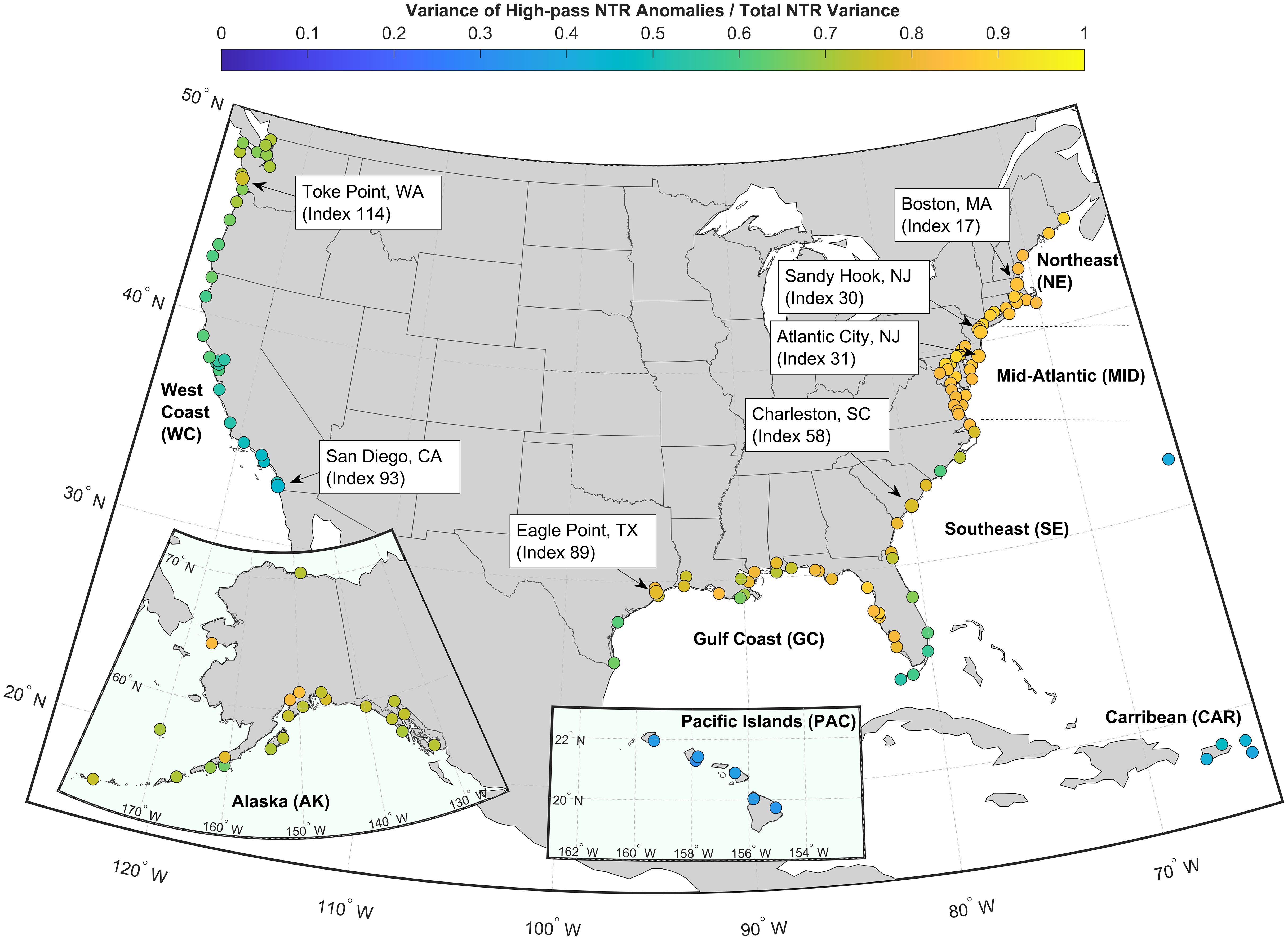
Figure 1. Fraction of the total ${\eta }_{NTR}$ variance explained by the $\eta {\text{'}}_{HIGH-PASS}$ at each NWLON station (Supplementary Table S1). Callouts refer to regions and specific stations discussed in the following subsections. Not displayed are: Sand Island, Midway Islands, Apra Harbor, Guam, Pago Pago, American Samoa, Kwajalein Island, and Wake Island (indices 7-11) which have fractional values equal to 0.50, 0.19, 0.14, 0.22, and 0.30, respectively.

Figure 2 shows considerable seasonal and spatial coherence of the $\eta {\text{'}}_{HIGH-PASS}$ fraction of ${\eta }_{NTR}$ variance. In general, $\eta {\text{'}}_{HIGH-PASS}$ variance dominates in the NE and MID year-round with 90% of the months in these regions having ratios greater than 0.72. Values are slightly more elevated during the fall and winter. The $\eta {\text{'}}_{HIGH-PASS}$ fraction in the SE and GC is also large but less so during the summer, especially in June. The relative contribution of $\eta {\text{'}}_{HIGH-PASS}$ variability increases in magnitude with increasing latitude along the WC (increasing indices) and into AK. For these regions, the $\eta {\text{'}}_{HIGH-PASS}$ variance explains a larger portion of the total during the summer and fall months. The ratio is smaller for nearly all months in South Florida (station indices 63-66) and along the southern WC (indices 93-100), especially September through December when the ratio drops to an average of 0.42. The relatively low fraction of $\eta {\text{'}}_{HIGH-PASS}$ variance for PAC and CAR is mostly seen year-round.

Figure 2

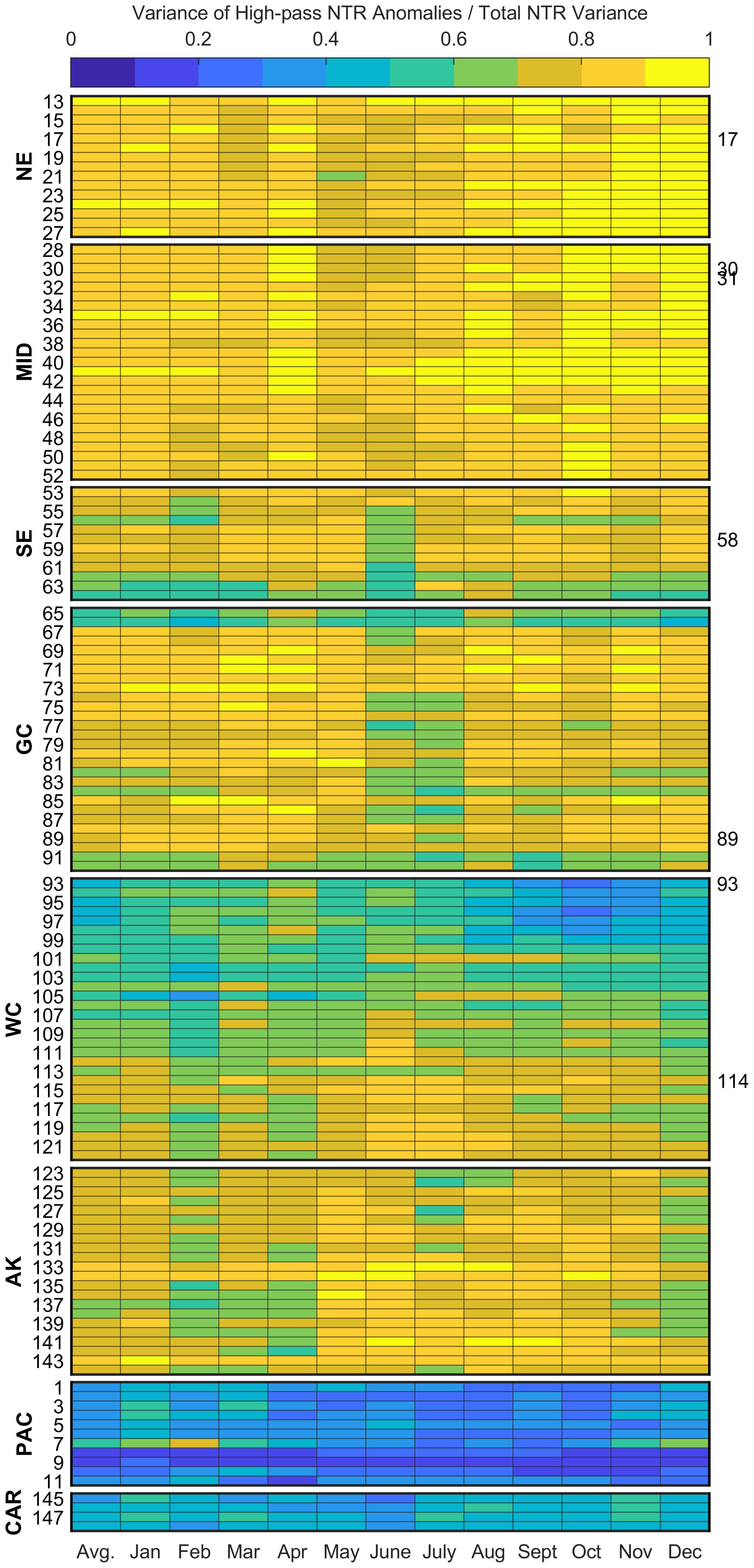
Figure 2. Fraction of the ${\eta }_{NTR}$ variance explained by the $\eta {\text{'}}_{HIGH-PASS}$ by month. The left y-axis shows the regions and station indices for each NWLON station (Supplementary Table S1), and the right y-axis indices refer to specific stations discussed in the results section (also see Figure 1). The total fraction (all months) for each station, also shown in Figure 1, is displayed in the first column. The regions include the: North East (NE), Mid-Atlantic (MID), Southeast (SE), Gulf Coast (GC), West Coast (WC), Alaska (AK), Pacific Islands (PAC), and Caribbean Islands (CAR). The callout stations are: Boston, MA (index 17), Sandy Hook, NJ (index 30), Atlantic City, NJ (index 31), Charleston, SC (index 58), Eagle Point, TX (index 89), San Diego, CA (index 93), Toke Point, WA (index 114).

3.1.2 Skewness and excess kurtosis of high-pass NTR anomalies

Figure 3 shows the generally parabolic relationship between the skewness (S) and excess kurtosis (K) of $\eta {\text{'}}_{HIGH-PASS}$, with data points showing that large amplitude (positive, or, less common, negative) values of S tend to coincide with large positive K. Moreover, for SGS distributions, S and K are bounded by the equation K ≥ 1.5S² – 0.5 (Sardeshmukh and Sura (2009); shown by the lower black line in Figure 3), which is the case for all stations in all months (Figures 3a, c) and in all regions (Figures 3b, d). PDFs with non-zero S are asymmetric and positive values of K indicate PDFs with heavier tails than a Gaussian PDF, for which S and K are zero.

Figure 3

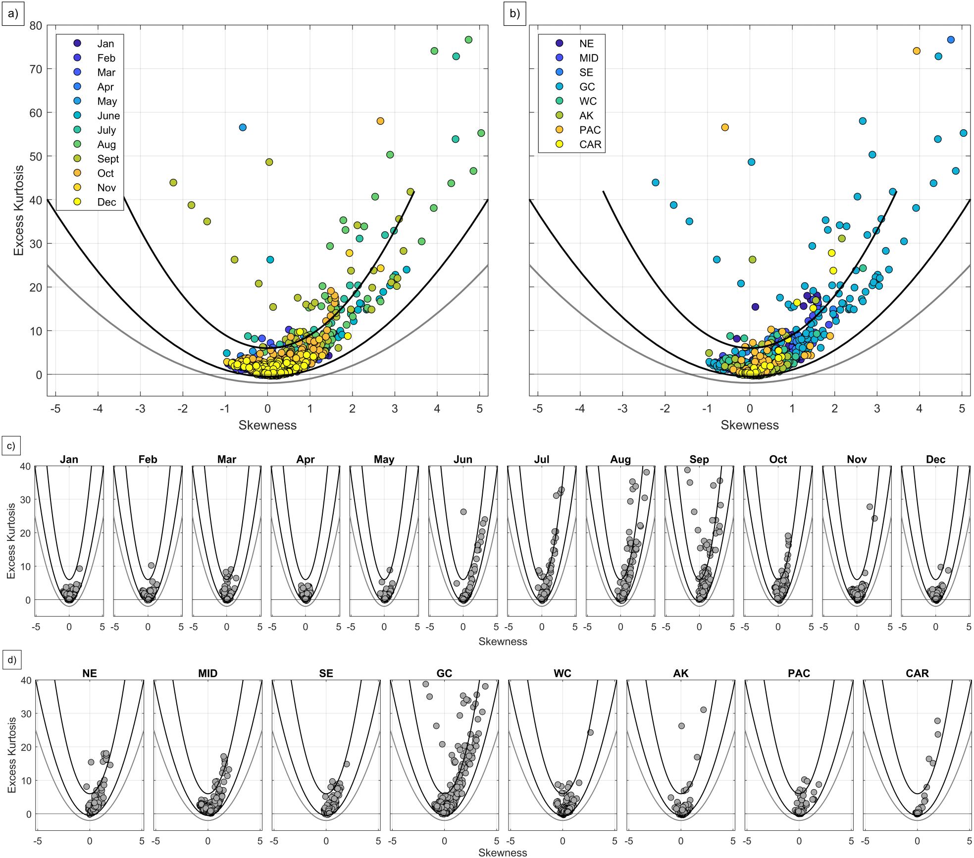
Figure 3. Skewness (S) and excess kurtosis (K) of the observed $\eta {\text{'}}_{HIGH-PASS}$ colored by (a) month and (b) region, and plotted specifically by (c) month and (d) region. Note, S and K are zero for Gaussian distributions. In each panel, the lower black line represents a theoretical lower bound on K of the form K = 1.5S² – Δ, where Δ = 0.5 is an arbitrary offset that addresses sampling errors in S and K estimation as well as the stationary assumption used in this study (Sardeshmukh and Sura, 2009). A universal lower bound on K, if K exists, is the parabola K = S² – 2 (grey line). The upper black line represents a theoretical upper bound on K if the fifth moment $x^5$ also exists (see Sardeshmukh et al., 2015 for details regarding theoretical limits of S and K). Three data points are out of range in these figures, corresponding to the tide gauges at Kahului, Hawaii in March, Panama City, Florida in July, and Apalachicola, Florida in July, due to exceedingly large values of K.

While there are some non-Gaussian characteristics present for all regions in all seasons, distributions are generally closer to Gaussian in winter and spring, with larger values of S and K during summer and fall (Figures 3a, c). Stations where the $\eta {\text{'}}_{HIGH-PASS}$ variance fraction is relatively high (Figure 2) tend to have heavy-tailed and skewed distributions, notably in the GC as well as the MID, NE, and SE, albeit with less extreme values (Figure 3d). In contrast, for Pacific region stations (WC and PAC), where the ${\eta }_{NTR}$ variability tends to be dominated by monthly time scales, distributions appear more Gaussian. For example, the WC distributions are more symmetric than others, with smaller values of S and often (although not always) smaller values of K. The CAR region is an exception: while its variability is also dominated by monthly time scales (Figure 2), it has many stations with skewed and heavy-tailed distributions (Figure 3). Each region also has some very heavy-tailed outliers, where K is so large that theoretically the fifth moment does not exist (values above the upper black line in Figure 3), occurring predominantly during July through September. This suggests that these distributions are unbounded in nature (Bingham et al., 1987).

3.2 Distributions of highpass NTR observations

In this section, we fit each station’s observed $\eta {\text{'}}_{HIGH-PASS}$ time series to an AR1 process (Equation 4 in section 2.3) and a CAM-noise process (Equation 5), separately for each month. Then, using the resulting parameters, we compute the corresponding AR1 and SGS PDFs, and compare them to the histograms determined for each station, using the RMSE difference (Equation 7) as our metric for goodness-of-fit.

3.2.1 Results for selected stations

We start by examining results for one station: Sandy Hook, New Jersey (index 30), where the $\eta {\text{'}}_{HIGH-PASS}$ variance dominates ${\eta }_{NTR}$ variance (0.87; Figure 1), especially during winter (Figure 2). The observed monthly histograms (shown by the grey bars in Figure 4) exhibit excess kurtosis and skewness compared to the AR1 PDF (purple), especially for August through October. In general, the AR1 PDF under-estimates the probability density both near the center of the distribution (where $\eta {\text{'}}_{HIGH-PASS}$ ≈ 0) and for the upper tail (shown in the insets). The non-Gaussian SGS PDF (yellow) better captures both the heavy-tailed and skewed characteristics of the distributions year-round, as shown by the negative RMSE differences for each month, with greatest improvement from late spring through early fall. The probability ratio of the 99^th percentile estimated by the SGS and AR1 PDFs (i.e., SGS/AR1) shows that the AR1 PDF estimates smaller tail probabilities for all months compared to the SGS PDF (Figure 4), with a ratio as large as 10.75 during September.

Figure 4

Figure 4. The distribution of the observed $\eta {\text{'}}_{HIGH-PASS}$ (grey bars) at Sandy Hook, NJ (index 30) for each month and the PDFs for the SGS (yellow) and AR1 (purple) with the 95% confidence intervals. The text refers to the difference (SGS minus AR1) in the root mean square error (RMSE) for the full and tail distribution. The insets show the upper tail distributions for anomalies greater than or equal to the 95^th percentile of the observed anomalies for each month. The teal dashed line represents the 99^th percentile of the observations and the ratio (SGS/AR1) represents the probability estimated by the SGS and AR1 PDFs. Note, the y-labels for the insets are shown on the right axis.

We next use five example stations selected from different coastal regions – Boston, Massachusetts (index 17), Charleston, South Carolina (index 58), Eagle Point, Texas (index 89), San Diego, California (index 93), and Toke Point, Washington (index 114) – to highlight representative differences between estimates of the AR1 and SGS PDFs for the months of March, June, September, and December (Figure 5). Overall, the SGS PDF outperforms or is comparable to the AR1 PDF at estimating the histogram for each station, except for Charleston in March (full distribution) and San Diego in June (upper tail). In these cases, the Gaussian distribution is already a good fit, and the SGS PDF reproduces it to within sampling uncertainty. The SGS PDF better approximates positively skewed and heavy-tailed characteristics (e.g., Boston, Charleston, and Toke Point) as well as negatively skewed distributions and light-tailed characteristics (e.g., Eagle Point in March and December). Both PDFs may under-estimate sample probabilities around the median for peaked (i.e., leptokurtic) distributions, such as Eagle Point in March; still, the SGS PDF remains a better fit.

Figure 5

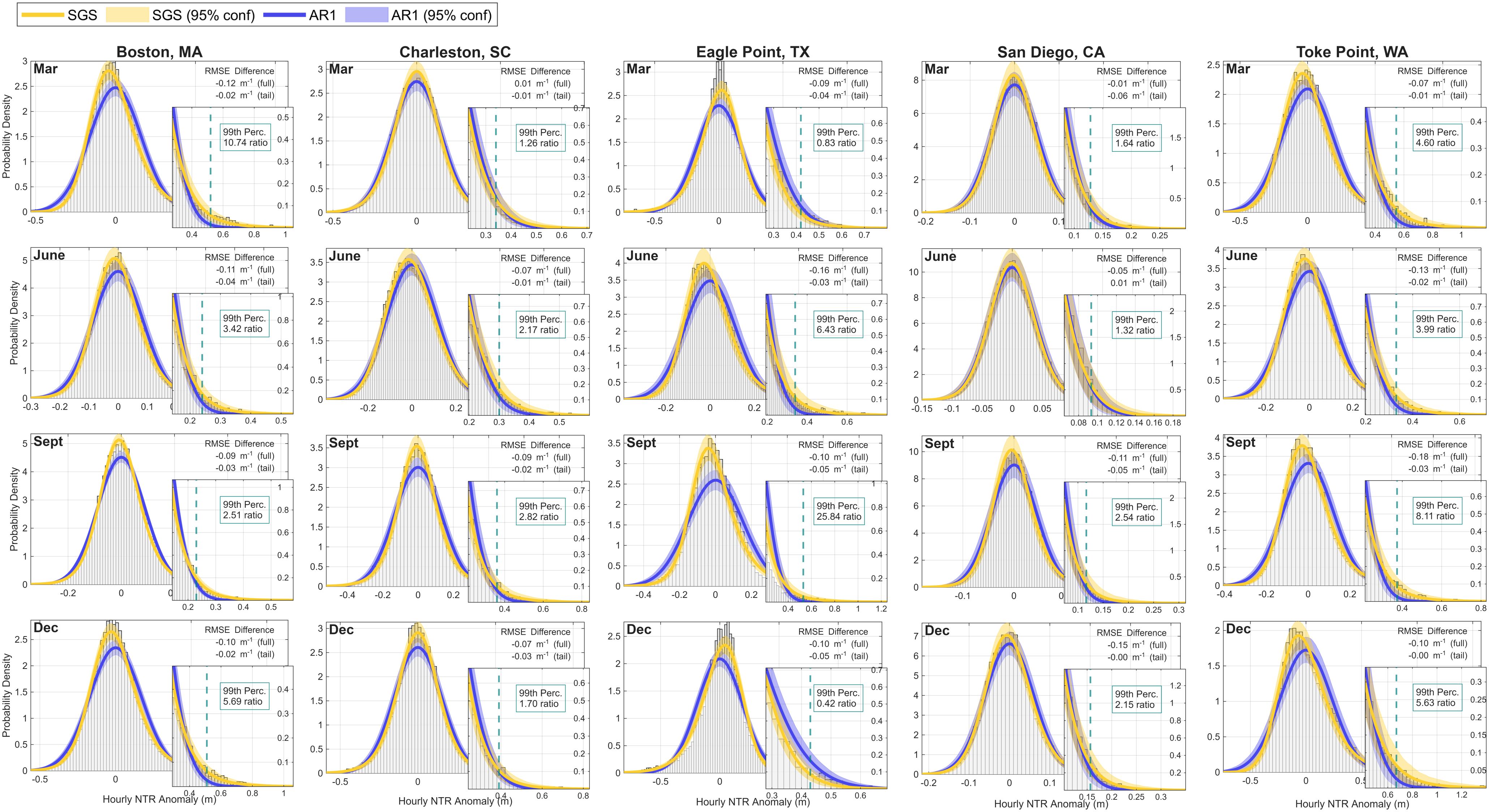
Figure 5. The distribution of the observed $\eta {\text{'}}_{HIGH-PASS}$ (grey bars) and the PDFs for the SGS (yellow) and AR1 (purple) with the 95% confidence interval at Boston, MA (index 17), Charleston, SC (index 58), Eagle Point, TX (index 89), San Diego, CA (index 93), Toke Point, WA (index 114) for the months of March, June, September, and December. The text refers to the difference (SGS minus AR1) in the root mean square error (RMSE) for the full and tail distribution. The insets show the upper tail distributions for anomalies greater than or equal to the 95^th percentile of the observed anomalies for each month at each station. The teal dashed line represents the 99^th percentile of the observations and the ratio (SGS/AR1) represents the probability estimated by the SGS and AR1 PDFs. Note, the y-labels for the insets are shown on the right axis.

3.2.2 Results for all stations

We next use the RMSE differences (Figure 6) to show that observed histograms are better approximated by the SGS PDFs than the AR1 PDFs for nearly every station, both averaged over the entire year (left-most column of each panel; 98.7% for the full distribution and 99.3% for the tail) and on a month-by-month basis (93.2% for the full distribution and 89.4% for the tail). The magnitudes of these improvements are strongly spatially correlated. For the East (West) Coast, improvements are typically largest in summer and fall (winter) (Figure 6a). While most stations and months have non-Gaussian distributions, a few have observed distributions that cannot be distinguished from a Gaussian distribution. These cases, identified by the Kolmogorov-Smirnov test (section 2) and indicated by cross-hatching in Figure 6, usually also have insignificant RMSE differences of either sign. The NE, MID, SE and GC regions have the largest percentage of months (all greater than 95%) with significant non-Gaussian characteristics. The WC and AK regions have greater than 89% and the PAC and CAR regions have around two thirds. Additionally, the SGS PDFs capture distributions for tide gauges located relatively far upriver (e.g., Philadelphia, PA; index 34, Washington D.C.; index 45, and Wilmington, NC; index 56) or in bays (e.g., Morgan’s Point to Rockport, TX; indices 88-91).

Figure 6

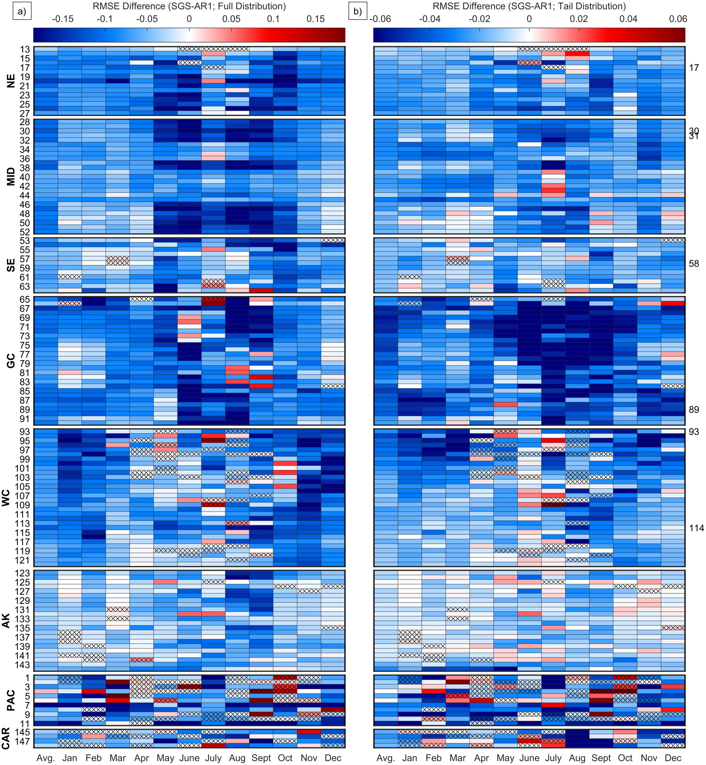
Figure 6. Difference (SGS minus AR1) in the root mean square error (RMSE) for (a) full and (b) tail distribution. RMSE is calculated between the SGS and AR1 PDFs and the observed $\eta {\text{'}}_{HIGH-PASS}$ distributions. The tail represents values greater than or equal to the 95^th percentile of the observed anomalies for each month at each station. The left y-axis shows the regions and station indices for each NWLON station (Supplementary Table S1), and the right y-axis indices refer to specific stations discussed in the results section (also see Figure 1). The average RMSE difference for all months is shown in the first column of each panel. Note the color bar range is different for the left and right panels. Blue squares represent a smaller RMSE, and therefore better fit to the histogram, when using the SGS PDF compared to the AR1 PDF, white is no change, and red indicates a larger RMSE. Cross-hatching represents where the Kolmogorov-Smirnov test failed to reject the null hypothesis that the observed $\eta {\text{'}}_{HIGH-PASS}$ come from a standard normal distribution at the 5% confidence level.

The SGS PDFs also generally improve estimates of the upper tail, and these improvements are also often spatially coherent in a manner somewhat similar to the full distributions (Figure 6b). The average error differences along the WC and into AK decrease at more northern stations (i.e., increasing in index value). Along the WC, the winter months again have the most PDF fit improvement. Both the PAC and CAR have varied RMSE differences for the tail of the distribution with both larger and smaller RMSE when using the SGS PDF that appear relatively random.

We find similar spatial and seasonal dependencies for the decorrelation timescale (${\tau }_c$), as well as the SGS parameters $E, g$, and $b$ and their relative contributions to the total CAM noise forcing variance (Supplementary Figure S2). More details are described in the Supplementary Section.

3.3 Evaluating high-water events

3.3.1 Comparison to AR1

As is evident in Figures 4 and 5, an important drawback of using an AR1 PDF to represent a heavy-tailed, skewed distribution is that the true tail probabilities may be over- or under-estimated. The tail probabilities estimated by the AR1 and SGS PDF also differ based on the chosen threshold (for example, compare the a) 95^th versus b) 99^th percentile in Figure 7). Using the 95^th percentile, the probability ratio is smaller than one (shown as yellow in Figure 7a) for most months at GC tide gauges and from winter through spring for the NE, MID, and SE; that is, $\eta {\text{'}}_{HIGH-PASS}$is less likely to exceed the 95% threshold based upon the SGS PDF than the AR1 PDF. Probability ratios exceeding one often occur along the WC and AK whereas the PAC and CAR have mixed results. There are also some cases where the SGS PDF did not improve upon the AR1 PDF, indicated by stippling in Figure 7a and, earlier, by red squares in Figure 6b. For those cases the probability ratio is generally close to 1.

Figure 7

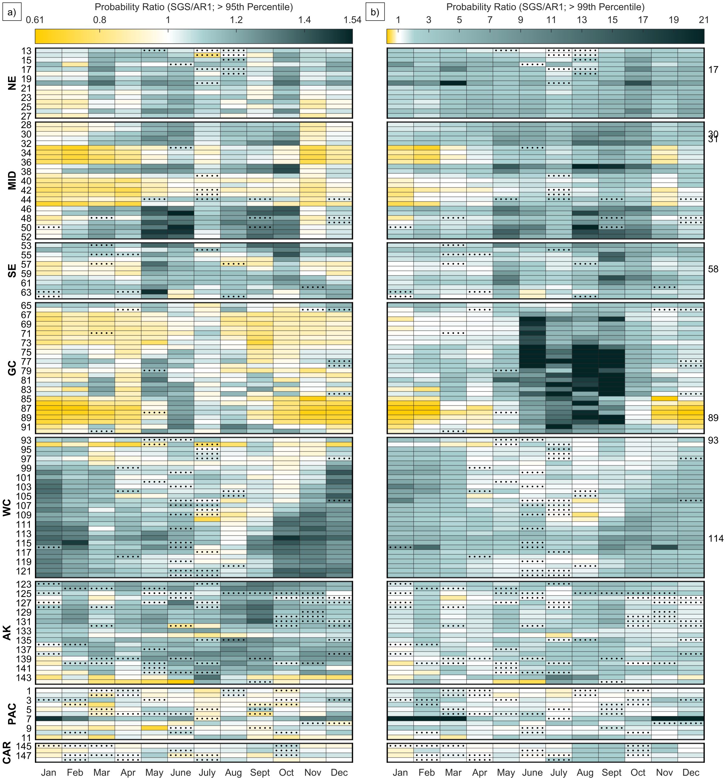
Figure 7. Ratio (SGS/AR1) of the estimated probability greater than the (a) 95^th and (b) 99^th percentile of the $\eta {\text{'}}_{HIGH-PASS}$ observations for each month at each station. The left y-axis shows the regions and station indices for each NWLON station (Supplementary Table S1). Indices on the right y-axis refer to the specific stations discussed in the results section. Yellow (teal) squares represent an AR1 estimated tail probability that is higher (lower) than that of an SGS and white is no difference. Stippling indicates when the RMSE for the AR1 PDF is less compared to the SGS PDF for the tail of the distribution (red squares in Figure 6b; note the column showing the yearly average is not included in this figure and the color bar range in (a, b) are different).

The range of probability ratios for the more extreme 99^th percentile threshold (Figure 7b) is larger compared to that for the 95^th percentile, and is generally greater than one for most tide gauges and months (shown as teal in Figure 7b). That is, $\eta {\text{'}}_{HIGH-PASS}$is more likely to exceed the 99% threshold based upon the SGS PDF than the AR1 PDF. The largest probability ratios occur in summer and fall in the GC, to a lesser degree in the NE, MID, and SE, and in the WC region during fall and winter. The largest ratios exceeding 20 (e.g., index 20 in Mar, index 7 during Nov-Mar, and others) occur when the AR1 PDF tail drops off, estimating probabilities near zero, while the SGS captures the heavy-tailed characteristics. In contrast, during winter months in the MID and GC, the SGS PDFs have negative skewness (Figure 3) and estimate smaller tail probabilities than expected from an AR1 PDF (yellow shading in Figure 7b). For cases where the SGS PDF does not improve upon the AR1 PDF (stippling in Figure 7b), the probability ratio average = 1.6.

3.3.2 Sensitivity to sampling

Up to this point, our analysis has been applied to 27-year long data records. We might ask if this record length is sufficient for our analysis, and relatedly whether the analysis of longer records might differ, especially for the stations (<10% of those analyzed here) with data records of 100 years or more. We explore this question by generating 2000 27-year samples (bootstrapping, with replacement) drawn from the entire 108-year Atlantic City record, choosing October as our test month. [As before, all monthly means are removed from the longer record so that it is effectively detrended. Note that no outliers (${\eta }_{NTR}$ exceeding ±10 standard deviations about the mean) are present in the October observations at this tide gauge.] To preserve the decorrelation timescale, we shuffle complete monthly datasets (i.e., all the hourly data within a given month; for example, October 2019) rather than hourly observations. We use these samples to generate 2000 PDFs determined from SGS fits, and 2000 PDFs determined by applying a Kernel Smoothing (KS) density approach to the raw histograms. These PDFs are compared to the histogram of the underlying 108-year record.

Both PDFs derived from the full record provide good approximations of the sample histogram (Figure 8a). The KS Density PDF fits small variations more closely, as might be expected, including the PDF bump for $\eta {\text{'}}_{HIGH-PASS}$ ~ 0.49 m (see inset). While values near the median ($\eta {\text{'}}_{HIGH-PASS}$ ~ 0 m) and the 99^th percentile ($\eta {\text{'}}_{HIGH-PASS}$ ~ 0.49 m) appear under-estimated by the mean SGS PDF, they still fall within the 95% confidence bounds. For the upper tail estimate, where data to constrain histogram fits and associated uncertainties are sparse (Figure 8b), the confidence bounds vary much more smoothly for the SGS PDF than the KS Density PDF. In fact, the SGS PDF might provide more stable estimates of high-water events, at least in contrast to the KS Density PDF, which may overfit small irregularities in the sample histogram extremes. Overall, these results suggest that the SGS PDF determined from the 27-year record used herein is representative of the longer record.

Figure 8

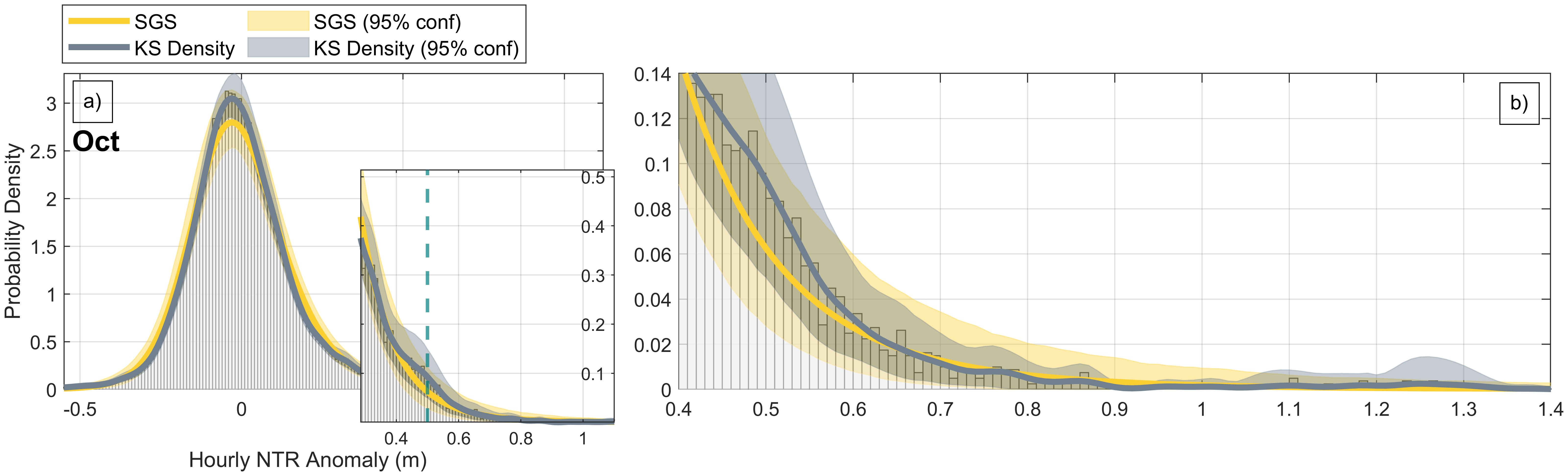
Figure 8. The histogram of the 108-year record of $\eta {\text{'}}_{HIGH-PASS}$ (grey bars) at Atlantic City, NJ (index 31) for the month of October and the SGS (yellow) and KS Density (grey) PDFs computed from the 2000 bootstrapped samples each with 27 years of data. The inset on panel (a) shows the upper tail distribution for anomalies greater than or equal to the 95^th percentile of the observed anomalies, and the teal dashed line represents the 99^th percentile of the observed (108 year) anomalies. Panel (b) shows the upper tail and high-water events in more detail.

3.3.3 SGS-derived recurrence intervals of extreme events

Finally, we show that the SGS distribution can provide robust recurrence interval estimates that are comparable to those using GEV methods. Figure 9 shows recurrence intervals of extreme events derived by applying GEV methods directly to the SGS synthetic data and to the raw observations, again using Atlantic City during October as an example. We use the block maxima method, selecting the maximum $\eta {\text{'}}_{HIGH-PASS}$ value within each October month from the 108-year dataset, to derive a GEV distribution and compute the recurrence intervals (black squares; Figure 9a). We then determine uncertainty in these recurrence intervals by applying the same GEV technique to each of the 2000 SGS synthetic time series, computed as described in section 2.4 except each is 108-years long.

Figure 9

Figure 9. The return level interval curve at Atlantic City, NJ (index 31) for the month of October estimated using the Generalized Extreme Value (GEV) method. (a) The monthly block maxima are computed from the full 108-year observations (black squares). The solid blue line represents the GEV computed from the 108-year monthly block maxima, and the solid yellow line represents the GEV computed from the SGS synthetic dataset derived from the 108-year hourly time series. Panels (b) through (e) show the same analysis but using 27-year data subsets starting in (b) 1911, (c) 1941, (d) 1969, and (e) 1997. The grey squares represent block maxima computed from each 27-year period, the dashed blue line represents the GEV computed from the 27-year monthly block maxima, and the dashed yellow line represents the GEV computed from the SGS synthetic dataset derived from the 27-year hourly time series. The SGS derived 95% confidence intervals for the 108-year dataset are also shown in each panel (light yellow swath). The variance (var), excess kurtosis (K), and skewness (S) for the 108 and 27-year datasets are also provided. Note the x-axis is in log-scale.

Figure 9a shows that the SGS-derived GEV (solid yellow line) is generally similar to the GEV computed from the 108 block maxima (solid blue line), although it estimates slightly lower water level anomalies at higher recurrence intervals. The block maxima observations, the GEV computed from the 108 observed block maxima, and the GEV computed from the synthetic SGS data all fall within the 95% confidence interval determined from the 2000 SGS synthetic time series (yellow swath). These results are consistent with Sardeshmukh et al. (2015), who showed that the SGS distribution tail is approximately of GEV form for certain block size conditions.

The sensitivity of these results to using a shorter sample is highlighted by repeating the analysis for different 27-year datasets, each drawn separately from the full time series beginning in either 1911 (Figure 9b), 1941 (Figure 9c), 1969 (Figure 9d), or 1997 (Figure 9e), where the start dates are not evenly spaced to account for years with incomplete or missing October data. For shorter recurrence intervals ≤ 10 October months (i.e., this is the return time for an event of this magnitude so 10¹ means it is expected every 10 years in October), the GEV computed directly from each 27-year observational sample (blue dashed lines) and from the SGS synthetic data (based upon new SGS fits determined from each 27-year time series; dashed yellow line) mostly follow the corresponding block maxima (grey squares), which can differ from the block maxima derived from the full record (black squares), seen in Figure 9a. For longer recurrence intervals (> 10 months), however, the two methods tend to diverge from the observed block maxima and each other. Also, recurrence intervals derived directly from observations (blue dashed line) have more sample-to-sample variation (e.g., the shape is more exponential in Figure 9d compared to Figure 9c) than those derived from the SGS fits.

As an additional significance test, we compare the recurrence intervals from each 27-year sample drawn from the SGS synthetic data to the range of expected random variation in recurrence intervals derived from the full 108-year record (yellow swath; note this is the same as in Figure 9a). We find that, except for the first period, each of our 27-year SGS-based recurrence interval estimates fall within the 95% confidence bounds from the 108-year record. Though not statistically significant, the dashed lines in the latter two time periods (Figures 9d, e) lie closer to the upper confidence bound, especially when compared with the earlier two time periods (Figures 9b, c). This suggests a potential increase in the water level extremes at the Atlantic City tide gauge during October over the course of the past century. This is consistent with the increase in skewness and excess kurtosis, although these are also not significantly different at the 95% confidence level (determined from 2000 realizations of 27-year periods pulled at random with replacement from the total 108-year record). While these changes in the recurrence intervals derived from the SGS synthetic data may not be significant, these results suggest that the relatively modest data needs for determining SGS distributions could be used to identify non-stationary $\eta {\text{'}}_{HIGH-PASS}$ distributions for other locations and/or seasons.

4 Concluding remarks

In this study, we determined distributions of observed $\eta {\text{'}}_{HIGH-PASS}$ at 148 tide gauges surrounding the United States, located in different regions and coastal environments (i.e., open ocean, within bays, estuaries, and near or upriver systems), and thus exposed to different forcing conditions. We have found that virtually all the distributions are significantly non-Gaussian, with skewed and heavy-tailed characteristics better estimated by the ‘Stochastically Generated Skewed’ (SGS) PDF than by a Gaussian PDF. (Results in the Pacific and Caribbean Islands are mixed.) These improvements, as measured by the RMSE of the PDF fits, are both spatially and seasonally coherent, most notably for summer and fall months along the Northeast, Mid-Atlantic, and Gulf Coasts and for winter months along the West Coast, both for the full distributions and for the upper tails alone. Arguably, the SGS distribution may be less advantageous as distributions become closer to normally distributed, such as in the Pacific Islands region. In these cases, although the SGS distributions include Gaussian distributions as a special case, some minor overfitting may occur. However, total η_NTR variance is also dominated by monthly variability at these stations (Figure 2), so that uncertainties in their high-pass distributions might be less impactful for many applications.

Accurate estimates of moderate to extreme high-water probabilities are essential for predicting flooding and its impacts on all time scales. Overall, the SGS PDFs improve the estimation of tail probabilities. Given the heavy-tailed, skewed histograms of $\eta {\text{'}}_{HIGH-PASS}$, the use of a Gaussian rather than an SGS distribution in NOAA’s HTF predictions could result in erroneous tail probabilities for HTF events, with an under-estimation that becomes larger for more extreme water level thresholds (e.g., 99^th percentile). Furthermore, the SGS PDF appears to provide good estimates of upper tail probabilities from record lengths of only a few decades, which allows for assessment of a great many tide gauge stations, especially compared to KS density methods which show some susceptibility to overfitting due to small sample sizes at the tails. The SGS distribution also provides comparable recurrence intervals of extreme events to GEV methods, while also capturing the full distribution. This provides probability estimates of more moderate water levels that could still be relevant to HTF, especially for increasing water levels. In addition to calculating recurrence intervals, the decorrelation timescale integrated into the governing equation for the SGS distribution can be used to identify the duration of extreme events (not shown; Xu et al., 2021).

To determine the full likelihood and recurrence intervals of HTF, the probabilities of $\eta {\text{'}}_{HIGH-PASS}$ estimated by the SGS distribution will need to be combined with the additional water level components (as in Equations 1 and 2). This could consist of convolving the $\eta {\text{'}}_{HIGH-PASS}$ PDF with the ${\eta }_M$ PDF and then adding in the tide prediction and trend component. Alternatively, the distributions of total water levels could be modeled directly, which for example, might require some modification of the deterministic portion of Equation 5 to account for tides. Thorough evaluation of these approaches may lead to improvements in the assessment of both observed and forecasted (e.g., ${\eta }_M$ derived from a seasonal forecast model ensemble) net HTF risk.

For Gulf Coast tide gauges during late summer to fall, we found that SGS distributions could be sensitive to tropical storms, which for any given location are, inevitably, poorly sampled over the 27-year record. Interestingly, the impact of excluding these extreme outlier events (amplitude > ± 10σ) was greater on the resulting SGS distributions near their medians than their tails. This is likely because while removing outliers will significantly impact K, which commonly has the largest error due to sampling, it also impacts other moments including S and variance. This suggests that replacing our ‘method of moments’ approach with a more rigorous approach that accounts for uncertainties in all three moments could improve our results (Martín et al., 2024), even with the presence of extreme outliers (Sardeshmukh et al., 2015). For example, maximum likelihood estimation (MLE) treats outliers so that they only have a 1/N (N = sample size) contribution to the log-likelihood of MLE, which limits their effect on parameter estimation. Continued testing is left for future work.

The SGS approach has a substantial number of advantages. It determines the parameters for a dynamical system that fits the observed time series. It provides a distribution for the observed histogram with parameters that can also be related to the parameters of the GEV distribution (Sardeshmukh et al., 2015). This means that we can use this dynamical system to generate synthetic time series of hourly $\eta {\text{'}}_{HIGH-PASS}$ (and potentially other physical variables) with the same statistical properties as the underlying observations. It can also be used to explore compound interactions between other processes (e.g., sea level, tides, waves, precipitation) that lead to flood-inducing total water levels (Anderson et al., 2019; Serafin et al., 2017). The dynamical system may be coupled with general circulation models (GCMs) ensemble forecasts to explore changes in climate scenarios. Additionally, since the SGS distribution can be readily interpreted in terms of dynamical processes, we could use it to characterize the past and current state of water level distributions and diagnose how probabilities may have evolved due to nonstationary data (e.g., decadal and climate variability).

One important question our results raise is: Which physical processes in the nearshore environment combine to result in CAM noise and therefore generate the SGS distributions we observe? Generally, $\eta {\text{'}}_{HIGH-PASS}$ are attributed to storm surge driven by wind-induced setup and atmospheric pressure anomalies (Bromirski et al., 2003; Pugh and Woodworth, 2014; Serafin et al., 2017), resulting from synoptic and mesoscale weather systems (World Meteorological Organization, 2011). While compound interactions between tides, wind waves, riverine flow, and precipitation modify storm surge (World Meteorological Organization, 2011), the dominant driver is wind-driven stress acting on the water surface, with the inverse barometer effect due to surface atmosphere pressure variations contributing approximately 10-15% (World Meteorological Organization, 2011). The time frame over which storm surge occurs can vary from a few minutes to several days with periods centered around approximately three hours (World Meteorological Organization, 2011); in comparison, for our study the $\eta {\text{'}}_{HIGH-PASS}$ decorrelation time scales range from 2 to 177 hours, with 95% between 5 and 63 hours. Moreover, surface winds may evolve more rapidly than changes in the sea surface height resulting from wind setup (Pugh and Woodworth, 2014). It seems possible then, at least in a shallow water framework, that CAM noise could result from the product of $\eta {\text{'}}_{HIGH-PASS}$ (the “slow” component) and the effect of wind-imparted stress on the ocean surface (the “fast” component). Additionally, although waves are not explicitly considered within this study, they may be sensed by NOAA tide gauges (Kirk et al., 2022; Sweet et al., 2015), and a state-dependence between wind stress and sea-state has been observed in some field experiments (Babanin and Makin, 2008; Dobson et al., 1994; Drennan et al., 2003; Reichl et al., 2014), although not in others (Yelland et al., 1998). A coastal shallow water model such as ADCIRC (Luettich and Westerink, 2004; Westerink et al., 2008) could be used as a diagnostic tool to explore these questions.

Data availability statement

The original contributions presented in the study are publicly available. This data can be found here: https://github.com/paigehovenga/SGS-Frontiers-Hovenga-2025.git. Further inquiries can be directed to the corresponding author/s.

Author contributions

PH: Writing – original draft, Writing – review & editing, Conceptualization, Formal analysis, Investigation, Methodology, Software, Visualization. MN: Writing – original draft, Writing – review & editing, Conceptualization, Investigation, Methodology, Project administration, Supervision. JA: Writing – review & editing, Methodology, Investigation. WS: Writing – review & editing, Methodology, Investigation. GD: Writing – review & editing. TX: Writing – review & editing. JC: Writing – review & editing. SS: Writing – review & editing. GC: Writing – review & editing, Methodology, Investigation.

Funding

The author(s) declare financial support was received for the research and/or publication of this article. PH, MN, JA, WS, GD, TX, JC, S-IS, and GC acknowledge the support from NOAA cooperative agreement NA22OAR4320151-T3-01S005 and PH, MN, JA, WS, GD, TX, JC, S-IS from the U.S. DoC/NOAA/Bipartisan Infrastructure Law (BIL).

Acknowledgments

The authors would like to thank Dr. Joseph Barsugli for discussions that improved the manuscript.

Conflict of interest

Author JC was employed by Ocean Associates, Inc.

The remaining authors declare that the research was conducted in the absence of any commercial or financial relationships that could be construed as a potential conflict of interest.

Generative AI statement

The author(s) declare that no Generative AI was used in the creation of this manuscript.

Any alternative text (alt text) provided alongside figures in this article has been generated by Frontiers with the support of artificial intelligence and reasonable efforts have been made to ensure accuracy, including review by the authors wherever possible. If you identify any issues, please contact us.

Publisher’s note

All claims expressed in this article are solely those of the authors and do not necessarily represent those of their affiliated organizations, or those of the publisher, the editors and the reviewers. Any product that may be evaluated in this article, or claim that may be made by its manufacturer, is not guaranteed or endorsed by the publisher.

Supplementary material

The Supplementary Material for this article can be found online at: https://www.frontiersin.org/articles/10.3389/fmars.2025.1618367/full#supplementary-material

References

Anderson D., Rueda A., Cagigal L., Antolinez J. A. A., Mendez F. J., and Ruggiero P. (2019). Time-varying emulator for short and long-term analysis of coastal flood hazard potential. J. Geophys. Res.: Oceans 124, 9209–9234. doi: 10.1029/2019JC015312

Crossref Full Text | Google Scholar

Arns A., Wahl T., Haigh I. D., Jensen J., and Pattiaratchi C. (2013). Estimating extreme water level probabilities: A comparison of the direct methods and recommendations for best practise. Coast. Eng. 81, 51–66. doi: 10.1016/j.coastaleng.2013.07.003

Crossref Full Text | Google Scholar

Babanin A. V. and Makin V. K. (2008). Effects of wind trend and gustiness on the sea drag: Lake George study. J. Geophys. Res.: Oceans 113, 2007JC004233. doi: 10.1029/2007JC004233

Crossref Full Text | Google Scholar

Bardet L., Duluc C.-M., Rebour V., and L’Her J. (2011). Regional frequency analysis of extreme storm surges along the French coast. Natural Hazards Earth Syst. Sci. 11, 1627–1639. doi: 10.5194/nhess-11-1627-2011

Crossref Full Text | Google Scholar

Bingham N. H., Goldie C. M., and Teugels J. L. (1987). Regular Variation (Encyclopedia Math. Appl. 27) Vol. 27 (Cambridge, UK: Cambridge University Pres).

Google Scholar

Box G. E., Jenkins G. M., Reinsel G. C., and Ljung G. M. (2015). Time series analysis: Forecasting and control (Hoboken, NJ: Wiley and Sons).

Google Scholar

Bromirski P. D., Flick R. E., and Cayan D. R. (2003). Storminess variability along the California Coast: 1858–2000. J. Climate 16, 982–993. doi: 10.1175/1520-0442(2003)016<0982:SVATCC>2.0.CO;2

Crossref Full Text | Google Scholar

Callahan J. A. and Leathers D. J. (2021). Estimation of return levels for extreme skew surge coastal flooding events in the Delaware and Chesapeake Bays for 1980–2019. Front. Climate 3. doi: 10.3389/fclim.2021.684834

Crossref Full Text | Google Scholar

Carr M. M., Gold A. C., Harris A., Anarde K., Hino M., Sauers N., et al. (2024). Fecal bacteria contamination of floodwaters and a coastal waterway from tidally-driven stormwater network inundation. GeoHealth 8, e2024GH001020. doi: 10.1029/2024GH001020

PubMed Abstract | Crossref Full Text | Google Scholar

Coles S. (2001). An introduction to statistical modeling of extreme values (4. printing) (London, UK: Springer).

Google Scholar

Collings T. P., Quinn N. D., Haigh I. D., Green J., Probyn I., Wilkinson H., et al. (2024). Global application of a regional frequency analysis to extreme sea levels. Natural Hazards Earth Syst. Sci. 24, 2403–2423. doi: 10.5194/nhess-24-2403-2024

Crossref Full Text | Google Scholar

Devlin A. T., Jay D. A., Talke S. A., and Zaron E. (2014). Can tidal perturbations associated with sea level variations in the western Pacific Ocean be used to understand future effects of tidal evolution? Ocean Dyn. 64, 1093–1120. doi: 10.1007/s10236-014-0741-6

Crossref Full Text | Google Scholar

Dixon M. J. and Tawn J. A. (1999). The effect of non-stationarity on extreme sea-level estimation. J. R. Stat. Society: Ser. C (Applied Statistics) 48, 135–151. doi: 10.1111/1467-9876.00145

Crossref Full Text | Google Scholar

Dobson F. W., Smith S. D., and Anderson R. J. (1994). Measuring the relationship between wind stress and sea state in the open ocean in the presence of swell. Atmosphere-Ocean 32, 237–256. doi: 10.1080/07055900.1994.9649497

Crossref Full Text | Google Scholar

Drennan W. M., Graber H. C., Hauser D., and Quentin C. (2003). On the wave age dependence of wind stress over pure wind seas. J. Geophys. Res.: Oceans 108, 2000JC000715. doi: 10.1029/2000JC000715

Crossref Full Text | Google Scholar

Dusek G., Sweet W. V., Widlansky M. J., Thompson P. R., and Marra J. J. (2022). A novel statistical approach to predict seasonal high tide flooding. Front. Mar. Sci. 9. doi: 10.3389/fmars.2022.1073792

Crossref Full Text | Google Scholar

Fant C., Jacobs J. M., Chinowsky P., Sweet W., Weiss N., Sias J. E., et al. (2021). Mere nuisance or growing threat? The physical and economic impact of high tide flooding on US road networks. J. Infrastruct. Syst. 27, 04021044. doi: 10.1061/(ASCE)IS.1943-555X.0000652

PubMed Abstract | Crossref Full Text | Google Scholar

Flood J. F. and Cahoon L. B. (2011). Risks to coastal wastewater collection systems from sea-level rise and climate change. J. Coast. Res. 274, 652–660. doi: 10.2112/JCOASTRES-D-10-00129.1

Crossref Full Text | Google Scholar

Ghanbari M., Arabi M., and Obeysekera J. (2020). Chronic and acute coastal flood risks to assets and communities in Southeast Florida. J. Water Resour. Plann. Manage. 146, 04020049. doi: 10.1061/(ASCE)WR.1943-5452.0001245

Crossref Full Text | Google Scholar

Ghanbari M., Arabi M., Obeysekera J., and Sweet W. (2019). A coherent statistical model for coastal flood frequency analysis under nonstationary sea level conditions. Earth’s Future 7, 162–177. doi: 10.1029/2018EF001089

Crossref Full Text | Google Scholar

Gold A. C., Brown C. M., Thompson S. P., and Piehler M. F. (2022). Inundation of stormwater infrastructure is common and increases risk of flooding in coastal urban areas along the US Atlantic Coast. Earth’s Future 10, e2021EF002139. doi: 10.1029/2021EF002139

Crossref Full Text | Google Scholar

Green P. J. and Silverman B. W. (1993). Nonparametric regression and generalized linear models: A roughness penalty approach (London, UK: Crc Press).

Google Scholar

Haigh I. D., Nicholls R., and Wells N. (2010). A comparison of the main methods for estimating probabilities of extreme still water levels. Coast. Eng. 57, 838–849. doi: 10.1016/j.coastaleng.2010.04.002

Crossref Full Text | Google Scholar

Hino M., Belanger S. T., Field C. B., Davies A. R., and Mach K. J. (2019). High-tide flooding disrupts local economic activity. Sci. Adv. 5, eaau2736. doi: 10.1126/sciadv.aau2736

PubMed Abstract | Crossref Full Text | Google Scholar

Hosking J. R. M. and Wallis J. R. (1997). Regional Frequency Analysis: An Approach Based on L-Moments. 1st ed (Cambridge, UK: Cambridge University Press). doi: 10.1017/CBO9780511529443

Crossref Full Text | Google Scholar

Hunter J. (2010). Estimating sea-level extremes under conditions of uncertain sea-level rise. Clim. Change 99, 331–350. doi: 10.1007/s10584-009-9671-6

Crossref Full Text | Google Scholar

Jacobs J. M., Cattaneo L. R., Sweet W., and Mansfield T. (2018). Recent and future outlooks for nuisance flooding impacts on roadways on the U.S. East Coast. Transp. Res. Record: J. Transp. Res. Board 2672, 1–10. doi: 10.1177/0361198118756366

Crossref Full Text | Google Scholar

Kirk K., Dusek G., Tissot P., and Sweet W. (2022). An approach to approximate wave height from acoustic tide gauges. J. Atmos. Oceanic Technol. 39, 721–738. doi: 10.1175/JTECH-D-20-0212.1

Crossref Full Text | Google Scholar

Li S., Wahl T., Barroso A., Coats S., Dangendorf S., Piecuch C., et al. (2022). Contributions of different sea-level processes to high-tide flooding along the U.S. Coastline. J. Geophys. Res.: Oceans 127, e2021JC018276. doi: 10.1029/2021JC018276

Crossref Full Text | Google Scholar

Li S., Wahl T., Fang J., Liu L., and Jiang T. (2023). High-tide flooding along the China coastline: past and future. Earth’s Future 11, e2022EF003225. doi: 10.1029/2022EF003225

Crossref Full Text | Google Scholar

Luettich R. and Westerink J. (2004). Formulation and Numerical Implementation of the 2D/3D ADCIRC Finite Element Model Version 44.XX.

Google Scholar

Martín A., Wahl T., Enriquez A. R., and Jane R. (2024). Storm surge time series de-clustering using correlation analysis. Weather Climate Extremes 45, 100701. doi: 10.1016/j.wace.2024.100701

Crossref Full Text | Google Scholar

Massey F. J. Jr (1951). The Kolmogorov-Smirnov test for goodness of fit. J. Am. Stat. Assoc. 46, 68–78. doi: 10.1080/01621459.1951.10500769

Crossref Full Text | Google Scholar

May C. L., Osler M. S., Stockdon H. F., Barnard P. L., Callahan J. A., Collini R. C., et al. (2023). “Chapter 9: coastal effects. Fifth national climate assessment,” in U.S. Global Change Research Program (Washington, DC, USA: U.S. Global Change Research Program). doi: 10.7930/NCA5.2023.CH9

Crossref Full Text | Google Scholar

Mazas F., Kergadallan X., Garat P., and Hamm L. (2014). Applying POT methods to the Revised Joint Probability Method for determining extreme sea levels. Coast. Eng. 91, 140–150. doi: 10.1016/j.coastaleng.2014.05.006

Crossref Full Text | Google Scholar

Mendes B. V. D. M. and Lopes H. F. (2004). Data driven estimates for mixtures. Comput. Stat Data Anal. 47, 583–598. doi: 10.1016/j.csda.2003.12.006

Crossref Full Text | Google Scholar

Méndez F. J., Menéndez M., Luceño A., and Losada I. J. (2007). Analyzing monthly extreme sea levels with a time-dependent GEV model. J. Atmos. Oceanic Technol. 24, 894–911. doi: 10.1175/JTECH2009.1

Crossref Full Text | Google Scholar

Moftakhari H. R., AghaKouchak A., Sanders B. F., and Matthew R. A. (2017). Cumulative hazard: The case of nuisance flooding. Earth’s Future 5, 214–223. doi: 10.1002/2016EF000494

Crossref Full Text | Google Scholar

Newman M., Alexander M. A., Ault T. R., Cobb K. M., Deser C., Di Lorenzo E., et al. (2016). The pacific decadal oscillation, revisited. J. Climate 29, 4399–4427. doi: 10.1175/JCLI-D-15-0508.1

Crossref Full Text | Google Scholar

Newman M., Wittenberg A. T., Cheng L., Compo G. P., and Smith C. A. (2018). The extreme 2015/16 el niño, in the context of historical climate variability and change. Bull. Am. Meteorol. Soc. 99, S16–S20. doi: 10.1175/BAMS-D-17-0116.1

Crossref Full Text | Google Scholar

NOAA (2025a). Notification of Updated Tidal Datums. Available online at: https://tidesandcurrents.noaa.gov/press/tidaldatum.html (Accessed November 21, 2024).

Google Scholar

NOAA (2025b). What is high tide flooding? Available online at: https://oceanservice.noaa.gov/facts/high-tide-flooding.html:~:text=High%20tide%20flooding%20occurs%20when,streets%20even%20on%20sunny%20days (Accessed November 21, 2024).

Google Scholar

Oelsmann J., Marcos M., Passaro M., Sanchez L., Dettmering D., Dangendorf S., et al. (2024). Regional variations in relative sea-level changes influenced by nonlinear vertical land motion. Nat. Geosci. 17, 137–144. doi: 10.1038/s41561-023-01357-2

PubMed Abstract | Crossref Full Text | Google Scholar

Pareja-Roman L. F., Orton P. M., and Talke S. A. (2023). Effect of estuary urbanization on tidal dynamics and high tide flooding in a coastal lagoon. J. Geophys. Res.: Oceans 128, e2022JC018777. doi: 10.1029/2022JC018777

Crossref Full Text | Google Scholar

Parker B. B. (2007). Tidal analysis and prediction (Silver Spring, MD: NOAA, NOS Center for Operational Oceanographic Products and Services), 378pp. doi: 10.25607/OBP-191

Crossref Full Text | Google Scholar

Pugh D. and Woodworth P. (Eds.) (2014). “Storm surges, meteotsunamis and other meteorological effects on sea level,” in Sea-Level Science: Understanding Tides, Surges, Tsunamis and Mean Sea-Level Changes (Cambridge University Press, Cambridge Core), 155–188. doi: 10.1017/CBO9781139235778.010

Crossref Full Text | Google Scholar

Reichl B. G., Hara T., and Ginis I. (2014). Sea state dependence of the wind stress over the ocean under hurricane winds. J. Geophys. Res.: Oceans 119, 30–51. doi: 10.1002/2013JC009289

Crossref Full Text | Google Scholar

Santamaria-Aguilar S. and Vafeidis A. T. (2018). Are extreme skew surges independent of high water levels in a mixed semidiurnal tidal regime? J. Geophys. Res.: Oceans 123, 8877–8886. doi: 10.1029/2018JC014282

Crossref Full Text | Google Scholar

Sardeshmukh P. D., Compo G. P., and Penland C. (2015). Need for caution in interpreting extreme weather statistics. J. Climate 28, 9166–9187. doi: 10.1175/JCLI-D-15-0020.1

Crossref Full Text | Google Scholar

Sardeshmukh P. D. and Penland C. (2015). Understanding the distinctively skewed and heavy tailed character of atmospheric and oceanic probability distributions. Chaos: Interdiscip. J. Nonlinear Sci. 25, 036410. doi: 10.1063/1.4914169

PubMed Abstract | Crossref Full Text | Google Scholar

Sardeshmukh P. D. and Sura P. (2009). Reconciling non-Gaussian climate statistics with linear dynamics. J. Climate 22, 1193–1207. doi: 10.1175/2008JCLI2358.1

Crossref Full Text | Google Scholar

Serafin K. A., Ruggiero P., and Stockdon H. F. (2017). The relative contribution of waves, tides, and nontidal residuals to extreme total water levels on U.S. West Coast sandy beaches. Geophys. Res. Lett. 44, 1839–1847. doi: 10.1002/2016GL071020

Crossref Full Text | Google Scholar

Shen S. and Kim K. (2020). Assessment of transportation system vulnerabilities to tidal flooding in Honolulu, Hawaii. Transp. Res. Record: J. Transp. Res. Board 2674, 207–219. doi: 10.1177/0361198120940680

Crossref Full Text | Google Scholar

Silverman B. W. (2018). Density Estimation for Statistics and Data Analysis. 1st ed (Boca Raton, FL: Routledge). doi: 10.1201/9781315140919

Crossref Full Text | Google Scholar

Solari S. and Losada M. Á. (2012). Unified distribution models for met-ocean variables: Application to series of significant wave height. Coast. Eng. 68, 67–77. doi: 10.1016/j.coastaleng.2012.05.004

Crossref Full Text | Google Scholar

Spanger-Siegfried E., Fitzpatrick M., and Dahl K. (2014). Encroaching tides: How sea level rise and tidal flooding threaten US East and Gulf Coast communities over the next 30 years (Cambridge, MA: Union of Concerned Scientists).

Google Scholar

Sukop M. C., Rogers M., Guannel G., Infanti J. M., and Hagemann K. (2018). High temporal resolution modeling of the impact of rain, tides, and sea level rise on water table flooding in the Arch Creek basin, Miami-Dade County Florida USA. Sci. Total Environ. 616–617, 1668–1688. doi: 10.1016/j.scitotenv.2017.10.170

PubMed Abstract | Crossref Full Text | Google Scholar

Sun Q., Dangendorf S., Wahl T., and Thompson P. R. (2006). Causes of accelerated High-Tide Flooding in the U.S. since 1950. npj Clim Atmos Sci. 6, 210. doi: 10.1038/s41612-023-00538-5

PubMed Abstract | Crossref Full Text | Google Scholar

Sura P., Newman M., and Alexander M. A. (2006). Daily to decadal sea surface temperature variability driven by state-dependent stochastic heat fluxes. J. Phys. Oceanogr. 36, 1940–1958. doi: 10.1175/JPO2948.1

Crossref Full Text | Google Scholar

Sweet W. (2021). 2021 State of High Tide Flooding and Annual Outlook (Silver Spring, MD: United States National Ocean Service, Center for Operational Oceanographic Products and Services). doi: 10.25923/MX62-RX21

Crossref Full Text | Google Scholar

Sweet W., Dusek G., Obeysekera J., and Marra J. J. (2018). Patterns and Projections of High Tide Flooding Along the U.S. Coastline Using a Common Impact Threshold (Silver Spring, MD: NOAA Technical Report NOS CO-OPS No. 086).

Google Scholar

Sweet W., Hamlington B. D., Kopp R. E., Weaver C. P., Barnard P. L., Bekaert D., et al. (2022). Global and regional sea level rise scenarios for the United States: updated mean projections and extreme weather level probabilities along US coastlines (Silver Spring, MD: National Oceanic and Atmospheric Administration, National Ocean Service, Center for Operational Oceanographic Products and Services).

Google Scholar

Sweet W. and Park J. (2014). From the extreme to the mean: Acceleration and tipping points of coastal inundation from sea level rise. Earth’s Future 2, 579–600. doi: 10.1002/2014EF000272

Crossref Full Text | Google Scholar

Sweet W., Park J., Gill S., and Marra J. (2015). New ways to measure waves and their effects at NOAA tide gauges: A Hawaiian-network perspective. Geophys. Res. Lett. 42, 9355–9361. doi: 10.1002/2015GL066030

Crossref Full Text | Google Scholar

Sweet W., Park J., Marra J., Zervas C., and Gill S. (2014). Sea level rise and nuisance flood frequency changes around the United States (NOAA Technical Report NOS CO-OPS&#x202F;; 073) (NOAA NOS; NOAA CO-OPS). Available online at: https://repository.library.noaa.gov/view/noaa/30823/noaa_30823_DS1.pdf (accessed November 21, 2024).

Google Scholar

Thompson P. R., Widlansky M. J., Hamlington B. D., Merrifield M. A., Marra J. J., Mitchum G. T., et al. (2021). Rapid increases and extreme months in projections of United States high-tide flooding. Nat. Climate Change 11, 584–590. doi: 10.1038/s41558-021-01077-8

Crossref Full Text | Google Scholar

Vitousek S., Barnard P. L., Fletcher C. H., Frazer N., Erikson L., and Storlazzi C. D. (2017). Doubling of coastal flooding frequency within decades due to sea-level rise. Sci. Rep. 7, 1399. doi: 10.1038/s41598-017-01362-7

PubMed Abstract | Crossref Full Text | Google Scholar

Wahl T., Haigh I. D., Nicholls R. J., Arns A., Dangendorf S., Hinkel J., et al. (2017). Understanding extreme sea levels for broad-scale coastal impact and adaptation analysis. Nat. Commun. 8, 16075. doi: 10.1038/ncomms16075

PubMed Abstract | Crossref Full Text | Google Scholar

Wand M. P. and Jones M. C. (1994). Kernel smoothing (New York, NY: CRC press).

Google Scholar

Wdowinski S., Bray R., Kirtman B. P., and Wu Z. (2016). Increasing flooding hazard in coastal communities due to rising sea level: Case study of Miami Beach, Florida. Ocean Coast. Manage. 126, 1–8. doi: 10.1016/j.ocecoaman.2016.03.002

Crossref Full Text | Google Scholar

Westerink J. J., Luettich R. A., Feyen J. C., Atkinson J. H., Dawson C., Roberts H. J., et al. (2008). A basin- to channel-scale unstructured grid hurricane storm surge model applied to Southern Louisiana. Monthly Weather Rev. 136, 833–864. doi: 10.1175/2007MWR1946.1

Crossref Full Text | Google Scholar

Williams J., Horsburgh K. J., Williams J. A., and Proctor R. N. F. (2016). Tide and skew surge independence: New insights for flood risk. Geophys. Res. Lett. 43, 6410–6417. doi: 10.1002/2016GL069522

Crossref Full Text | Google Scholar

World Meteorological Organization (2011). Guide to Storm Surge Forecasting (No. 1076) (Geneva Switzerland: World Meteorological Organization).

Google Scholar

Xu T., Newman M., Capotondi A., and Di Lorenzo E. (2021). The continuum of northeast Pacific marine heatwaves and their relationship to the tropical Pacific. Geophys. Res. Lett. 48, 2020GL090661. doi: 10.1029/2020GL090661

Crossref Full Text | Google Scholar

Yelland M. J., Moat B. I., Taylor P. K., Pascal R. W., Hutchings J., and Cornell V. C. (1998). Wind stress measurements from the open ocean corrected for airflow distortion by the ship. J. Phys. Oceanogr. 28, 1511–1526. doi: 10.1175/1520-0485(1998)028<1511:WSMFTO>2.0.CO;2

Crossref Full Text | Google Scholar