Projected shifts in the spatio-temporal distribution of larval chub mackerel (Scomber japonicus) under climate change in the western North Pacific

We projected the effects of the climate change on the abundance and biomass distribution of chub mackerel (Scomber japonicus) eggs and larvae by developing and applying an individual-based model (IBM) based on a regional ocean circulation model for the western North Pacific. While building upon established IBM frameworks, this study provides the first high-resolution projection of larval chub mackerel biomass and distribution under climate change in this region. Our IBM tentatively suggested that the distribution of chub mackerel larvae extended from the southern waters of the East China Sea to the Japanese coastal areas, the Korea Strait and Japan/East Sea, following the Tsushima warm current, a branch of the Kuroshio current. The larval chub mackerel biomass during the 2010s was higher from April to June, peaking in May, in the East China Sea. Despite the greater uncertainty, the preliminary results of our IBMs projected that, by the 2050s, the increased water temperature, driven by global warming, will increase the larval mackerel biomass and shift their distribution north to the Yellow Sea and the Japan/East Sea. To enhance the model performance, international collaborative research among regional countries is recommended, particularly for conducting comprehensive ichthyoplankton surveys in the western North Pacific and sharing fisheries data. We expect that our model projections will contribute to the development of fisheries policy and management plan for adaptation to climate change in the region.

1 Introduction

Chub mackerel, Scomber japonicus, are widely distributed in the western North Pacific with two stocks, the Tsushima Warm Current (TWC) stock in the East China Sea (ECS), Yellow Sea (YS) and Japan/East Sea (JES) and the Pacific stock in the Pacific coast of Japan (Jung, 1977; Watanabe et al., 2002; Yamada et al., 2007; Yukami et al., 2009). The TWC stock shows seasonal migrations, moving northward to the JES and YS through the Korea Strait (KS) after the spring-summer spawning period from February to June and then southward back to their spawning grounds in the ECS and the KS during autumn-winter (Cha et al., 2002; Hiyama et al., 2002; Hwang et al., 2008; Li et al., 2014b; Yamada et al., 2007; Yukami et al., 2009). They mainly lay their eggs at water temperatures from 15 to 22°C within 25 m depth, and their larvae are distributed at water temperatures from 13 to 22°C in the upper 50-m depths (Fritzsche, 1978; Kim et al., 2019; Sassa and Tsukamoto, 2010; Yukami et al., 2009).

The Kuroshio Current (KC) and its branch, the Tsushima Warm Current (TWC), have been cited as a significant variable for understanding the recruitment and spatio-temporal variability of distribution for fisheries species in the Korean waters (Hwang and Jung, 2012; Jung, 2008; Jung et al., 2013, 2014; Lee et al., 2021). While the temperatures in the Korean peninsula and its adjacent sea waters have significantly increased by global warming during the past 40 years (Jung, 2008), 6 of 12 major fish species showed a significant relationship between the mean monthly-latitude of the catch distribution of fishes and the water temperatures from 1984 to 2010 (Jung et al., 2014). Although the mean latitude of chub mackerel had not shown a significant trend of northward shift, zonal shifts with respect to the change of water temperature at 30 m depth were reported by Jung et al. (2014).

The recruitment of marine fish is highly sensitive to oceanographic and biotic variabilities during early-life stages, which affects growth, survival, and ultimately population dynamics (Houde, 1987, 2009; Letcher et al., 1996). The survival during these stages are especially vulnerable to the environmental variability because of their limited swimming ability for moving to a favorable habitat for growth and survival (Blaxter, 1992; Brochier et al., 2009; Gilbert et al., 2010; Norcross and Shaw, 1984). For chub mackerel, sea temperature and ocean currents are critical environmental conditions during the larval stages. Larval growth and developmental rates are temperature-dependent, which also affects recruitment (Go et al., 2020; Guan et al., 2023; He et al., 2024; Kamimura et al., 2015; Li et al., 2012). Furthermore, as eggs and larvae are planktonic and unable to swim actively, their dispersal is largely governed by ambient current direction and velocity (Li et al., 2012, 2014; Wang et al., 2023). These mechanisms directly affect their spatial distribution and exposure to favorable or unfavorable conditions, ultimately influencing survival and recruitment success.

Individual-based model (IBM) is a type of modeling approach that simulates the dynamics of a population as being composed of discrete individual organisms by emulating the behavior and interactions of individual fish (Deangelis et al., 1991; Deangelis and Grimm, 2014). IBMs avoid the limitations of traditional population models, which violate basic principles of biology by treating many individual organisms as a single entity and not considering their heterogeneity (Huston et al., 1988; Van Winkle et al., 1993). IBMs integrate the various levels in the traditional hierarchy of ecological processes by showing that all levels can be understood through the direct and indirect interactions of individual organisms with each other and the environment (Huston et al., 1988). IBMs can be used to test a hypothesis, answer a research question or solve an applied problem such as the variation among individuals, their life cycle changes, local interactions, and adaptive behavior, which could not be properly represented in population-level numerical models (Deangelis and Grimm, 2014). IBMs are highly adaptable to a wide range of time and space scales, allowing description of biological processes for both individuals and aggregated populations (Megrey and Hinckley, 2001). IBMs have been increasingly applied in fisheries science since the 1990s to investigate and evaluate the trajectory, connectivity, and recruitment of fish, particularly their early-life stages (Christensen et al., 2007; Hinckley et al., 1996; Letcher et al., 1996; Werner et al., 2001).

Researchers have also used IBMs for this purpose in the western North Pacific (Chang et al., 2015; Guan et al., 2023; Guo et al., 2022; Jung et al., 2016; Li et al., 2014a, 2012, 2014; Okunishi et al., 2009). For chub mackerel, Li et al. (2012) estimated the larval growth rate as a function of water temperature and food concentration and the larval mortality as a function of body length and growth rate to simulate the early-life ecology by developing the individual-based model of chub mackerel (IBM-CM). Li et al. (2014a) studied the impact of a typhoon on larval dispersal, growth, and mortality in the ECS with respect to its intensity, path, and duration by using IBM-CM. Li et al. (2014b) extended their IBM-CM to five stages from spawning and egg incubation to juveniles with length up to 13 cm and a time scale up to 4 months to examine the impact of water temperature change and drifting to different areas on their incubation, metamorphosis time and mortality. Guo et al. (2022) first developed an IBM for chub mackerel in the western North Pacific with a bioenergetics module for evaluating the effects of environmental factors on the growth, migration, and recruitment of chub mackerel. Guan et al. (2023) investigated the spatio-temporal distribution and patterns of growth and survival rates of chub mackerel and analyzed the relationship of the distribution, growth, and survival rate with the marine environment by developing of an IBM for chub mackerel larvae and juveniles.

Here, we attempted to evaluate and project the effect of the climate-driven changes in the ocean circulation on the biomass distribution of chub mackerel during the early-life stages in the western North Pacific. For this purpose, we developed a bio-physical coupled IBM simulating early-life stage processes (growth, mortality, and dispersal) under dynamically downscaled present (2010s) and future (2050s) oceanographic conditions based on the IPCC AR5 RCP 8.5 scenario, which was selected to explore a high-emission, worst-case pathway and assess potential upper-bound impacts on the species (Ipcc, 2014). While several previous IBM studies have examined the ecological dynamics of chub mackerel under present-day or short-term environmental variability, no study has yet assessed their long-term responses to projected climate change in this region. We hypothesized that rising ocean temperatures will increase larval biomass and cause a northward shift in their distribution, with implications for early-life survival and recruitment. The results are expected to provide new insight into how climate-driven oceanographic changes will reshape the spatio-temporal distribution of larval chub mackerel biomass and production, supporting regional policy makers to develop adaptive fisheries management plans in the face of climate change and global warming.

2 Materials and methods

2.1 Model description

We developed a bio-physical coupling individual-based model for Tsushima Warm Current stock of chub mackerel during early-life stages (IBM-TCM) in the western North Pacific (118°00′–143°00′E and 20°00′–52°00′N; Figure 1). We adopted the physical model of our study area, Regional Ocean Modeling System (ROMS), which simulated 3-dimensional fields of water temperature, salinity, density, and current speed (Go et al., 2025), and incorporated biological processes such as growth and mortality of mackerel.

Figure 1

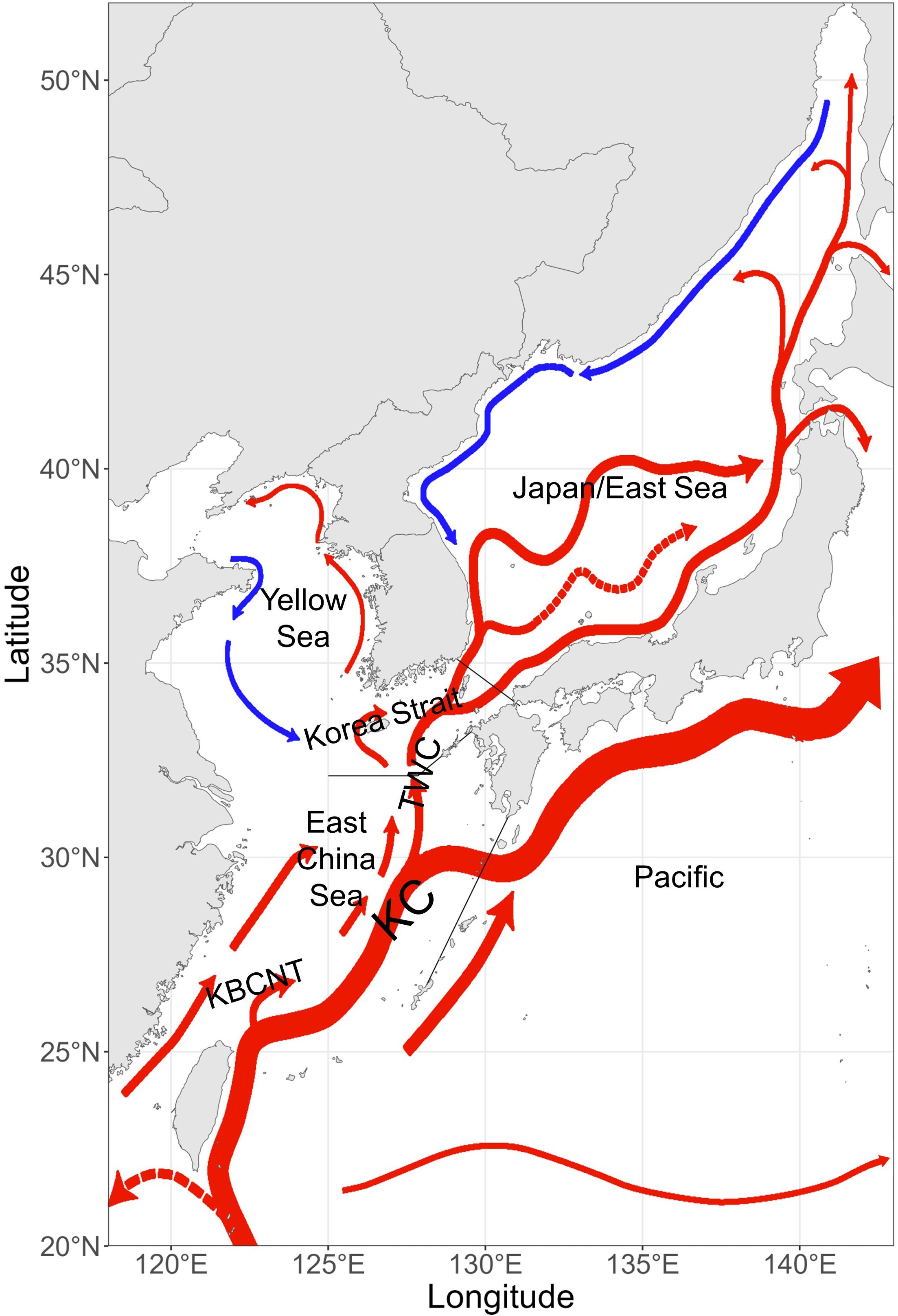
Figure 1. Study area and major currents (blue, cold current; red, warm current; KC, Kuroshio Current; KBCNT, Kuroshio Branch Current north of Taiwan; TWC, Tsushima Warm Current).

The IBM-TCM tracked the movement and population dynamics of “super-individuals”, a modeling unit representing a group of identical individuals experiencing the same physical environment. This method, following Scheffer et al. (1995) and Megrey and Hinckley (2001), allows efficient simulation of large populations while retaining spatial heterogeneity by assigning unique environmental histories to each cohort. Biological parameters (e.g., growth and mortality) are applied uniformly across super-individuals, but divergence in their developmental trajectories emerges from spatially variable environmental inputs.

The model was designed to simulate the early-life stages of chub mackerel, by defining individual organisms and assigning state variables (such as body length, location, and age) and behavior rules (including spawning, growth, and mortality) to each super-individual. The physical environment was an input into the model, with daily and 3-dimensional spatial variation. We coupled the physical and biological models using a Lagrangian particle tracking method, with eggs and larvae interacting with the environment during passive drift, which affects their growth and development. The model simulated the spatio-temporal changes of eggs and larvae with the physical environment and individual variables updated in each loop to generate environmental and biological data on a daily basis. While the model did not consider active behaviors such as diel vertical migration or ontogenetic movement, we attempted to capture the first-order effects of physical forcing on larval drift and exposure, which primarily drive the early-life stage dynamics of pelagic fish. A detailed workflow of the IBM-TCM, including data inputs, coupling steps, and outputs, is presented in Supplementary Materials (Supplementary Figure S1).

2.2 Physical model

We took the ROMS developed by Go et al. (2025), that covered the entire Korean waters and its adjacent seas with a horizontal resolution of 1/12° and 30 vertical sigma layers (118°00′–143°00′E and 20°00′–52°00′N). The detailed structure of this model was described by Go et al. (2025). This model simulated ocean dynamics with sufficient precision, based on the Semi-spectral Primitive Equation Model and the terrain-following model structure by applying the S-coordinate Rutgers University Model. The model was designed to simulate ocean conditions 2010–2059 under climate change conditions, based on the modeling results from the IPCC Fifth Assessment Report (IPCC AR5).

Because the AR5 model did not provide suitable open boundary conditions for a regional ocean model, a Pacific-scale model (104°00′E–104°00′W and 20°00′S–65°00′N) with a horizontal resolution of 1°~1/6° and 30 vertical sigma layers was first run to generate initial and open boundary conditions for the regional-scale model. This large-scale simulation was driven by atmospheric forcing from the ECHAM6 RCP 85 scenario provided by the Max Planck Institute and produced monthly average values of sea surface height, temperature, salinity, and velocity. The same atmospheric forcing data were applied to the northwestern Pacific model.

The model runs included monthly mean river discharge of the Changjiang (Yangtze River) from Datong station, and tidal effect was included using ten tidal harmonics from a global tide simulation to represent surface height and depth-averaged velocity boundary conditions. Although the ROMS output was not explicitly bias-corrected, we assumed that they could reproduce large-scale seasonal sea temperature patterns and hydrographic structures consistent with observed oceanographic data (Go et al., 2025).

The ROMS stored the daily-averaged model results of water temperature, salinity, density, and the current speeds at each layer, and we used the daily-averaged water temperatures, densities, and velocities of the current in x, y, and z directions. To evaluate the reliability of the ROMS, we validated the modeled sea temperatures at multiple depths by comparing them with the observed oceanographic data from the Korea Oceanographic Data Center (KODC).

We chose the RCP 8.5 high-emission scenario to represent an upper-bound climate forcing pathway and to evaluate the potential response of larval chub mackerel under strong ocean warming. This choice was made due to data availability at the time of model construction and the high-resolution downscaling already completed for this scenario.

2.3 Biological model of chub mackerel

2.3.1 Spatio-temporal distribution of eggs

We assumed the initial spatio-temporal distribution of chub mackerel eggs for IBM-TCM based on the spawning ground index (SGI) proposed by Go et al. (2025) and the randomly-selected initial dates from 1 February to 30 June. We assumed that their initial distributions of vertical-locations are uniform at 1–10 m depth, because chub mackerel eggs were reported to abundantly distribute within 10 m depth, and reach up to 20 m in later stages (Fritzsche, 1978).

We assumed the spawning proportion in day d (P_d) follows the normal distribution function with a mean of 16 April and a standard derivation of 30 days, resulting in approximately 99% of spawning occurring between February and June. This assumption was based on Yukami et al. (2009), which estimated that the spawning period based on the monthly changes in the gonadosomatic index (GSI). The GSI, defined as the ratio of gonad weight to body weight, is a standard index of reproductive activity and was used to constrain the seasonal spawning pattern in the model.

We arbitrarily assigned a total of 10¹⁰ eggs per year, and the daily number of eggs on day d (N_d) was calculated by multiplying the daily spawning proportion and the total number of eggs per year. The total number of cohorts was assumed 10,000 per year, and the initial number of cohorts i spawned on the day sd_i ($N_{s{d}_i,i}$) was calculated by randomly dividing the initial number of eggs on the day sd_i ($N_{s{d}_i}$) by the number of cohorts spawned on the same days. We provided the detailed coordinates of the initial egg release locations and their monthly distribution in Supplementary Materials (Supplementary Data S1).

2.3.2 Early-life stages

We calculated the daily hatching progress rate of chub mackerel eggs using the incubation time (t_h, day) varying with water temperature T (°C) reported by Hunter and Kimbrell (1980). If the sum of the rates was over 1, we assumed that the mackerel hatched.

We adopted the differential equation of the temperature-dependent Gompertz-Laird growth equation for chub mackerel larvae proposed by Go et al. (2020) and calculated by Go and Jung (2023), in which they assumed that the length of the hatched larva was 0.31 cm and the length at metamorphosis was 1.5 cm in fork length (FL), as follows:

$$dL=0.0028e^{0.0971T}L\ln (38.5126/L)$$

where T is the water temperature (°C).

We calculated the cm FL of chub mackerel in a cohort i at day d (L_d,i), as follows:

$$\{\begin{array}{ll}{L}_{d,i}=0.11\hfill & ifs{d}_i\le d<h{d}_i\hfill \\ L_{d,i}=0.31+d{L}_{h{d}_i,i}\hfill & ifd=h{d}_i\hfill \\ L_{d,i}=L_{d-1,i}+d{L}_{d-1,i}\hfill & ifd>h{d}_i\hfill \end{array}$$

where sd_i is spawned day of cohort i, hd_i is hatched day of cohort i, and $d{L}_{h{d}_i,i}$ is the increment length at the time of excess hatching progress rate of cohort i in hatched day hd_i.

We applied the size-specific instantaneous mortality of chub mackerel (Z, day^-1) proposed by Go and Jung (2023),

$$Z=0.1097/L$$

To derive their vertical movement, we adopted the specific gravity of chub mackerel (Lee et al., 2017) eggs was 1.0246 g cm^-3, and that of larvae was

$${\rho }_p=0.076L+0.9962$$

2.3.3 Biomass

We derived the number of chub mackerel in a cohort i at day d,

$$N_{d,i}=N_{s{d}_i,i}\exp (-\sum _{m=s{d}_i}^{d-1}{Z}_{m,i})=N_{s{d}_i,i}\exp (-\sum _{m=s{d}_i}^{d-1}0.1097/L_{m,i})$$

where $N_{s{d}_i,i}$ is the initial number of cohorts i spawned on the day sd_i.

To estimate the biomass of chub mackerel, we converted the derived FL to the wet weight (W) in grams using the length-weight relationship reported by Choi et al. (2000).

$$W=0.0044L^{3.3362}$$

We estimated the biomass of chub mackerel,

$$B=WN$$

We stopped the simulation of each individual when chub mackerel metamorphosed, i.e., reaching 1.5 cm FL. Daily biomass distribution maps were generated by averaging the values of all of the cohorts for each grid of the model domain.

2.4 Bio-physical coupling

Because of their limited swimming ability, chub mackerel during early-life stages drift passively with the oceanic currents and are affected by the environmental conditions of the ambient water. Therefore, we assumed that their horizontal movement speed is equivalent to the current speed of their ambient water mass. We applied the Stokes′ regime to estimate their sinking speed by mass-density difference (Parada et al., 2003):

$$v_s=\frac{1}{24}g{R}_s^2\frac{{\rho }_p-{\rho }_w}{{\rho }_w}{\nu }^{-1}\ln (\frac{2R_l}{R_s}+\frac{1}{2})$$

where g is the gravitational force (m/s²), ρ_w is the density of their ambient water (g/cm³), ρ_p is the specific gravity of chub mackerel (g/cm³), R_l and R_s are major and minor axis length of the chub mackerel body (m), and ν is effective viscosity (0.01 m²/s). This effective viscosity was originally applied by Parada et al. (2003) to represent additional biological drag effects of fish eggs and larvae. A comparison with the results using the commonly applied physical kinematic viscosity (≈ 1 × 10⁻⁶ m²/s) is provided in Appendix B.

To apply the Stokes′ regime, we assumed that the shape of chub mackerel eggs is a sphere with a diameter of 1.1 mm (Hunter and Kimbrell, 1980; Kramer, 1960), and the shape of chub mackerel larvae is spheroid with the major axis of chub mackerel larvae is R_l = L and the minor axis is R_s = 0.088L^1.38 (Mendiola et al., 2007). We calculated their vertical movement speed by adding the sinking speed and the vertical current speed. We estimated their daily hatching progress rate and growth as a function of the ambient water temperature derived from the ROMS output data.

2.5 Model validation

To diagnose our IBM, we qualitatively compared the model results with the observed data of chub mackerel larvae in past studies (Kim et al., 2019; Lee et al., 2016; Sassa and Tsukamoto, 2010). The distribution of chub mackerel larvae in March of 2004 and 2005 was observed in the southern part of ECS (Sassa and Tsukamoto, 2010), and the surveys in April and May 2013, and May and June 2014 provided their distribution in the coast of Jeju Island (Lee et al., 2016). Kim et al. (2019) collected chub mackerel larvae in the Korean waters in May and June of 2016 and 2017. The comparison was conducted based on qualitative agreement in the spatial and seasonal distribution patterns between our simulation outputs and those previously reported. In addition, to provide a quantitative assessment of model performance, we used digitized observational data extracted from Lee et al. (2016) and Kim et al. (2019). We selected these datasets because they provide maps with digitizable larval abundance and correspond to years, months and regions covered by our simulations. Other available datasets, such as Kim et al. (2019) 2016 surveys, were excluded due to unclear distinction of abundance levels, which would hinder meaningful comparison. Observed values were aggregated onto 0.5° × 0.5° grid cells to match the spatial resolution of the model outputs, and log-transformed and normalized to account for scale differences and extreme values. We then calculated the Pearson correlation between model-predicted relative abundances and digitized observational data, allowing us to quantitatively assess the matching in their spatial distribution patterns.

Additionally, to evaluate the biological realism of our stage duration by water temperature, we compared its outputs with relationships reported in previous studies (Hunter and Kimbrell, 1980; Go et al., 2020). For this comparison, we simulated stage durations between 15 and 22°C, and conducted Kolmogorov-Smirnov (K-S) tests to assess statistical differences. This allowed us to determine whether the model’s developmental timing is consistent with previously established growth-temperature relationships.

2.6 Projected spatio-temporal changes in larval biomass distribution

To investigate the potential impacts of global warming on the early-life stages (< 1.5 cm FL) of chub mackerel, we conducted a comparative analysis of model outputs between the 2010s (2010–2019) and the 2050s (2050–2059) under the IPCC AR5 RCP 8.5 scenario. Specifically, we examined monthly biomass distribution patterns, and calculated the stage duration (days), the average daily mortality (day^-1), and the cumulative mortality from spawned to the completion of the metamorphosis. Furthermore, we assessed the spatial shifts in larval distribution by calculating the biomass-weighted mean latitudes and longitudes for each month of the two time periods.

To account for stochastic variability in the initial spatial distribution of eggs, we performed 10 replicate simulations using different random seeds. Monthly biomass and other metrics were computed as the mean values across simulations, and the variability was expressed as standard deviations or 95% confidence intervals.

2.7 Sensitivity analyses

To evaluate the robustness of our projections, we conducted additional sensitivity analyses addressing uncertainties in temperature forcing and the larval mortality coefficient. We first implemented a medium-warming surrogate scenario, representing an intermediate level between historical and RCP 8.5 conditions, to assess the sensitivity of larval projections to varying water temperature because only a single climate realization (RCP 8.5) was available. To do this, we calculated the mean monthly temperature differences between the 2010s and 2050s for each depth and grid cell, and reduced the mean warming effect by 50% while preserving the temporal variability and circulation fields of the 2050s. We then re-ran the IBM under this perturbed forcing with the same biological settings as the baseline, and compared the resulting larval biomass and the spatial centroid of the larval distribution between the RCP 8.5 and surrogate scenario.

In addition, to assess the sensitivity to variations in the model coefficients, we varied the mortality rate and growth coefficient by ±20%, and the spawning period by ±2 weeks while keeping all other parameters constant. These ranges were chosen to reflect the typical uncertainty associated with larval survival, growth, and spawning period in individual-based models. We then re-ran the simulations for the 2010s and 2050s under these perturbed settings, and compared the resulting larval biomass and spatial centroids with those from the baseline to evaluate the robustness of our model outcomes.

2.8 Data processing and visualization

We used R statistical software (R Core Team, 2024) for data processing and statistical analyses, and the ggplot2 (Wickham, 2016) and rnaturalearth (Massicotte et al., 2023) packages for spatial visualizations and maps.

3 Results

3.1 Hydrographic conditions

Our regional circulation model projected an overall warming trend of the ocean surface from the 2010s to the 2050s, except in the northern part of the JES, where a slight cooling was predicted (Figure 2). The TWC was projected to intensify, resulting in a stronger northward inflow of warm waters.

Figure 2

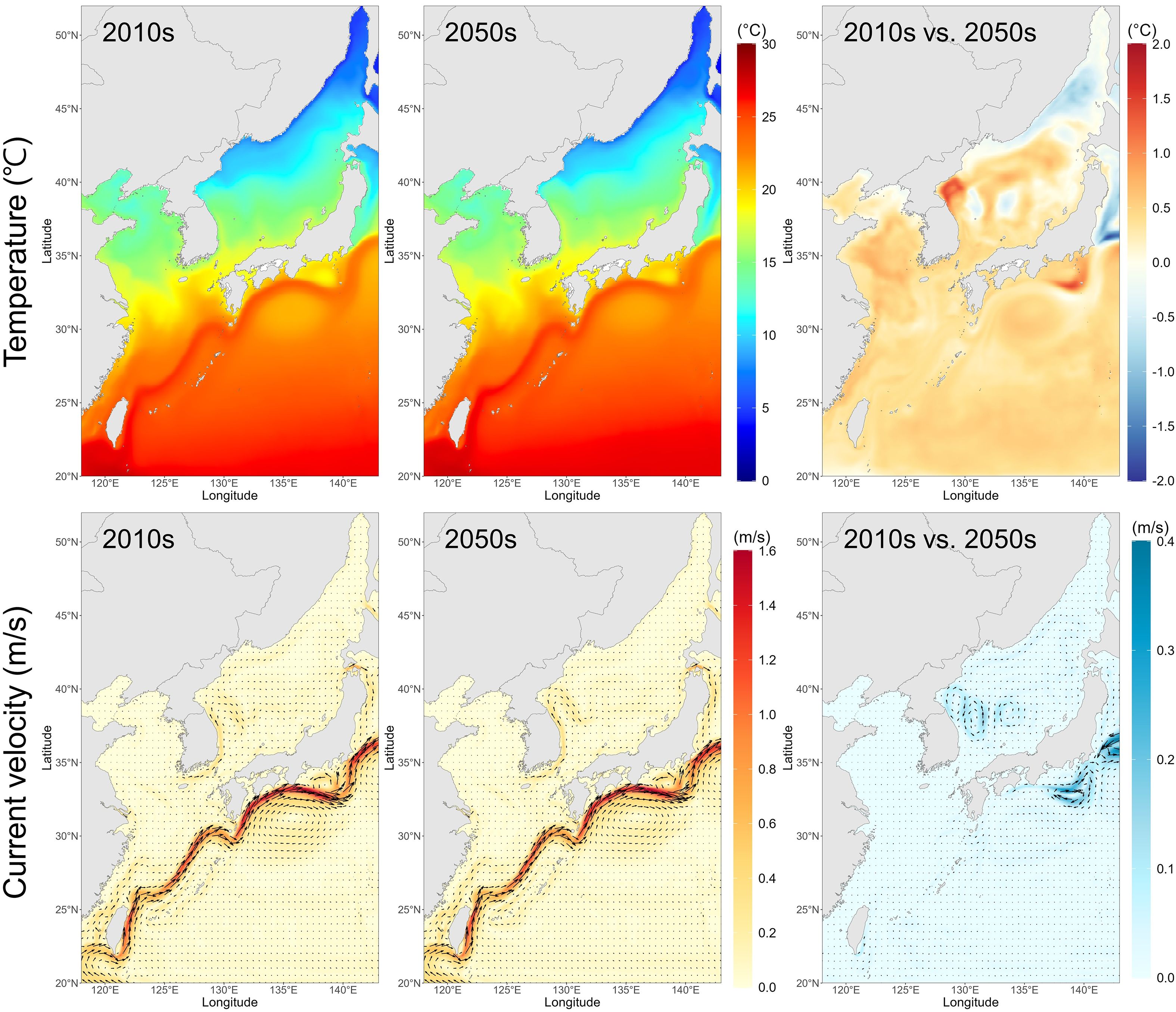
Figure 2. Water temperatures and oceanic current velocities averaging from 0 to 20-m depth, predicted for the 2010s and the 2050s, and differences between the two periods.

The depth-specific changes in water temperature and current are summarized in Table 1 (detailed in Supplementary Table S1). The water temperature increased across all depths (1–75 m), with an average rise of 0.29–0.33°C. Notably, the surface temperature was projected to increase by 0.29°C, and the subsurface layers such as 20–50 m depths projected similar increases (0.32–0.33°C). The projected surface current speed slightly increased to both zonal and meridional directions (+0.12 and +0.105 cm/s), whereas at depths below 10 m, a general weakening of current speed was projected, especially in the meridional direction.

Table 1

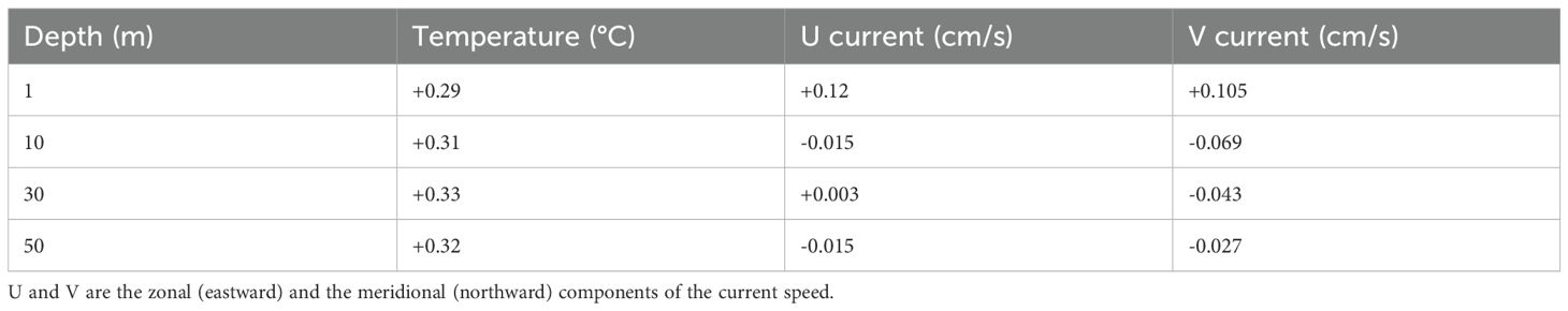
Table 1. Summary of projected changes in water temperature and current speed at selected depths in the study area from the 2010s (2010–2019) to the 2050s (2050–2059).

Table 2 shows the monthly water temperature changes during the spawning period (February–June) at 1–10 m depths, where chub mackerel eggs are mostly distributed. More detailed temperature profiles are available in Supplementary Table S2. The projected temperature at 1 m depth rose from an average of 14.79°C in February to 23.10°C in June during the 2010s, and from 15.16°C to 23.63°C in the 2050s. The largest increase was projected in May (0.60°C), highlighting the potential for accelerated larval growth and development during peak spawning season.

Table 2

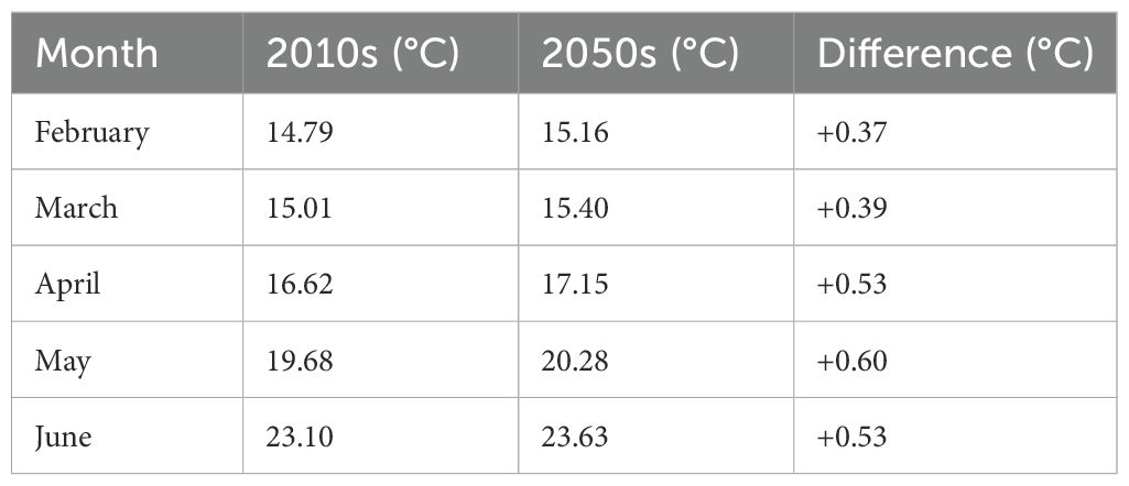
Table 2. Projected monthly water temperature at 1 m depth, summarizing warming trends during the spawning season for the 2010s (2010–2019), the 2050s (2050–2059), and differences between the two periods in the study area.

These results summarize the projected seasonal changes in water temperatures and oceanic currents during the spawning season of chub mackerel, with the largest temperature increase in May and an overall intensification of the TWC.

The reliability of these modeled temperature patterns was assessed by comparing them with bimonthly in-situ data from the Korea Oceanographic Data Center (KODC) across depths from 0 to 75 m. As detailed in Appendix A, the ROMS results showed no significant difference in warming trends compared to observations, confirming that the model effectively captured the seasonal and vertical thermal structure in the study area. Furthermore, bias and root mean square error (RMSE) statistics for sea surface temperatures from February to June indicated relatively minor mean biases (-0.28 to +1.53°C) and RMSE values of < 2.73°C across the ECS, KS/YS, and ES.

3.2 Changes in larval biomass

Our IBM-TCM projected monthly changes in the biomass of larval chub mackerel, with a peak in May in the 2010s and the 2050s (Figure 3). In the 2010s, the projected biomass increased from February to May and declined after June, with highest biomass concentrated in the East China Sea (ECS). The projected total biomass increased month-by-month and peaked in May (Table 3), with full regional breakdowns provided in Supplementary Table S3.

Figure 3

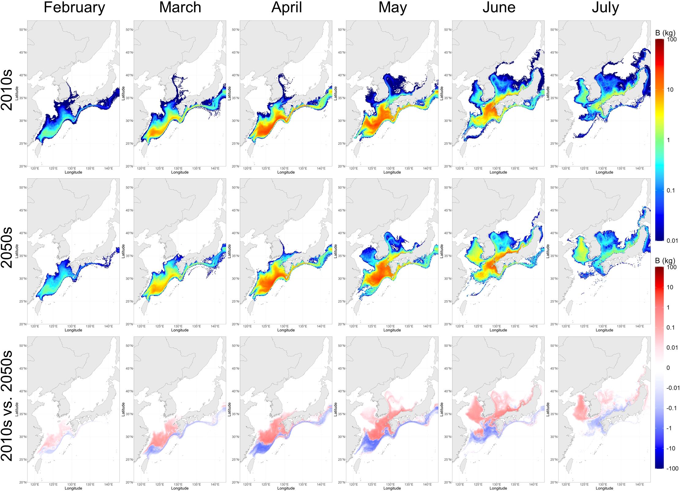
Figure 3. Monthly biomass distribution of larval chub mackerel (Scomber japonicus), averaged for the 2010s and the 2050s, and the differences between the two periods predicted by the individual-based model. The unit is kilogram per 0.1°×0.1°.

Table 3

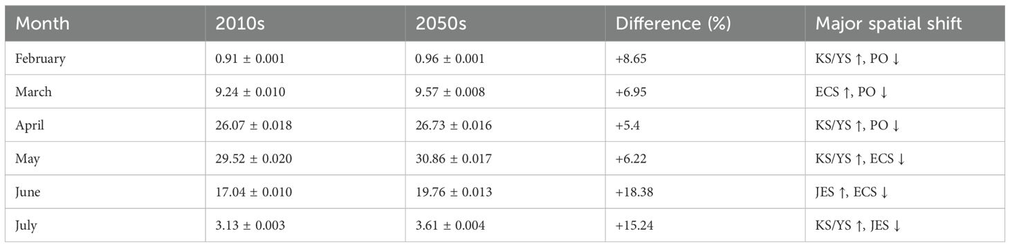
Table 3. Summary of total larval biomass (scaled index) of chub mackerel (Scomber japonicus) by month and major regional changes between the 2010s (2010–2019) and the 2050s (2050–2059) with standard deviation (ECS, East China Sea; PO, Pacific Ocean; KS, Korea Strait; YS, Yellow Sea; JES, Japan/East Sea).

Projections for the 2050s under the IPCC AR5 RCP 8.5 scenario showed an increased overall biomass with a notable shift in the spatial distribution. Projected biomass increased in the northern regions (KS/YS and JES) while decreasing in the ECS and the Pacific Ocean (PO). For instance, the biomass proportion in the KS/YS region increased from 6.99% in May (2010s) to 15.96% (2050s), while it decreased in the ECS from 77.34% to 71.29% (Supplementary Table S3). The overall larval biomass from February to July increased by 8.88% in the 2050s compared to the 2010s (Table 3). These results indicated a northward shift in spawning success and larval retention, likely driven by warming conditions and intensified current dynamics projected in the physical model.

Stage duration and mortality rates were projected to remain relatively stable. The average duration was 21.77 ± 4.59 days in the 2010s, and 21.52 ± 4.63 days in the 2050s. Similarly, the projected average daily mortality (day^-1) during early-life stages was 0.1684 ± 0.0079 in the 2010s, and 0.1681 ± 0.0085 in the 2050s, with cumulative mortality estimated at 3.65 ± 0.69 and 3.60 ± 0.70, indicating minimal change in early-life survivorship despite spatial redistributions.

3.3 Spatio-temporal shift in larval distribution

The biomass-weighted centroids of larval chub mackerel distribution were projected to gradually shift from the ECS toward the northeast from February to July, ranging from 28.61°N, 125.72°E to 35.18°N, 130.51°E in the 2010s and from 28.93°N, 125.55°E to 36.37°N, 128.57°E in the 2050s (Figure 4). On average, the centroids in the 2050s were located 0.72°N farther north than in the 2010s, and notably, the July centroid in the 2050s showed a northwestward shift from 33.81°N, 129.23°E to 36.37°N, 128.57°E, in contrast to the continued northeastward shift in the 2010s from 32.62°N, 129.02°E to 35.18°N, 130.51°E.

Figure 4

Figure 4. Biomass-weighted centroids of larval chub mackerel (Scomber japonicus) distribution from February to July in the 2010s (left) and the 2050s (right). Ellipses denote 95% confidence intervals derived from 10 simulation replicates (Feb.: solid line, Mar.: dashed, Apr.: dotted, May: dotdash, Jun.: longdash, Jul.: twodash).

3.4 Sensitivity analyses of model parameters

The surrogate medium-warming scenario, representing 50% of the mean projected warming, produced larval distributions broadly consistent with those under the RCP 8.5 baseline. The monthly larval biomass showed negligible variation between the two scenarios, with only marginally lower values under the perturbed forcing (Supplementary Table S4). However, the spatial centroid of larval distribution shifted slightly southward and westward compared with the RCP 8.5 baseline, particularly during the peak spawning months (May–July). For example, in May the centroid under the perturbed forcing was located at 30.86°N and 127.61°E, compared with 30.86°N and 127.87°E in the baseline. Similarly, in July the centroid shifted from 36.37°N to 35.82°N.

To further examine model sensitivity, we varied the mortality rate by ±20% while keeping all other parameters constant, and compared the resulting total larval biomass and the spatial centroid of the larval distribution between the 2010s and 2050s (Supplementary Table S5). In the 2010s, reducing mortality by 20% increased larval biomass by 188% relative to the control, accompanied by a slight northward (+0.15°N) and eastward (+0.19°E) shift in the biomass centroid. Conversely, a 20% increase in mortality decreased larval biomass by 63% compared to the control, with the centroid shifting marginally southward (-0.15°N) and westward (-0.20°E). In the 2050s, larval biomass responded similarly, increasing under reduced mortality (+184%) and decreasing under increased mortality (-63%), while centroid shifts remained small (0.11°E and -0.11°E, 0.13°N and -0.11°N).

We also perturbed the temperature-dependent growth coefficient by ±20% while maintaining constant all other parameters (Supplementary Table S6). In the 2010s, a 20% decrease in the growth coefficient resulted in a 28% reduction in larval biomass relative to the control, accompanied by a slight eastward (+0.28°) and northward (+0.11°) shift in the centroid. Conversely, an increase of 20% in the growth coefficient resulted in an increase in biomass of ca. 28%, and a shift of the centroid by 0.22° westward and 0.09° southward. In the 2050s, biomass showed similar responses, with a decrease of 28% and an increase of 28% under reduced and increased growth, respectively. Centroid shifts remained minimal, with values less than 0.2° in longitude and 0.1° in latitude.

We further evaluated model sensitivity to spawning phenology by shifting the mean spawning period by ±2 weeks (Supplementary Table S7). In the 2010s, advancing spawning by two weeks decreased larval biomass by 31% relative to the control and shifted the centroid southwestward (-0.42°E and -0.65°N). Conversely, delaying spawning by two weeks reduced biomass by 67% and shifted the centroid northeastward (+0.62°E and +0.25°N). In the 2050s, biomass showed a comparable response, with a decrease of 33% in the earlier spawning period and 68% in the later spawning period, while centroid shifts were moderate (-0.45°E and 0.28°E, -0.86°N and 0.16°N).

4 Discussion

4.1 Comparison with past studies

Our IBM-TCM showed that the chub mackerel eggs laid from February to May were primarily transported toward the PO under the influence of the KC, whereas those less affected by the KC remained mainly in the ECS. The chub mackerel eggs laid in June were predominantly distributed in the KS and transported to the JES under the influence of the TWC. The currents flowing toward the Yellow Sea (YS) were weaker than those directed toward the JES or the PO, resulting in fewer larval chub mackerel moving toward the YS. Chub mackerel eggs were spawned at water temperatures ranging from 15 to 22°C (18.50 ± 1.54°C), and the larvae subsequently experienced varying ambient water temperatures until completing metamorphosis.

The mean stage duration from the hatch to the completion of the metamorphosis for eggs spawned at water temperatures ranging from 29.5 days at 15–16 to 16.7 days at 21–22°C (Figure 5). The projected decrease in stage duration with increasing temperature aligns with previous studies (Go et al., 2020; Hunter and Kimbrell, 1980). However, our result was significantly different from the line reported by Hunter and Kimbrell (1980) (K-S test, p < 0.05), while not differing from the curve estimated by Go et al. (2020) (p = 0.18). This difference may be attributed to the fact that our IBM-TCM simulated the dynamic exposure of larvae to daily varying water temperatures, thereby capturing more realistic thermal histories during development compared to static temperature experiments in earlier studies.

Figure 5

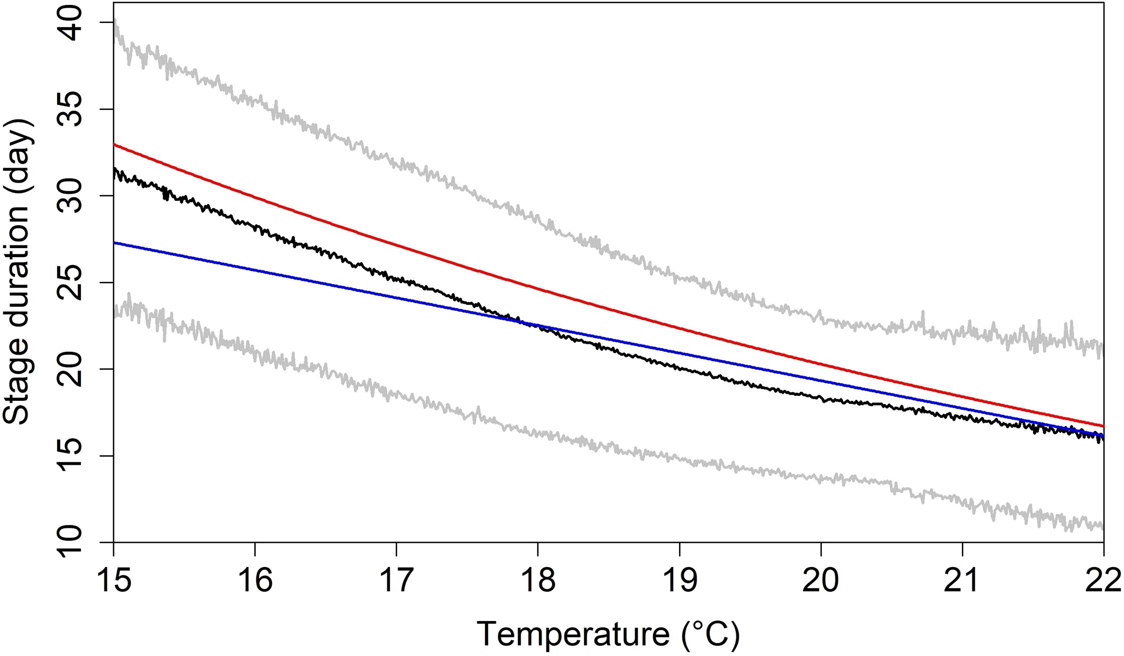
Figure 5. Stage duration in days of chub mackerel (Scomber japonicus) by the water temperature which they were spawned (black line) and its 95% confidence intervals (grey lines), and the stage duration in days by the water temperature which they were exposed during larvae stages in the past studies (Hunter and Kimbrell, 1980: blue line, Go et al., 2020: red line).

We compared the monthly-averaged biomass distribution of chub mackerel larvae predicted by the IBM-TCM with observational ichthyoplankton survey data from Sassa and Tsukamoto (2010); Lee et al. (2016), and Kim et al. (2019). Due to the limited availability of survey data during the peak spawning season, a comprehensive validation across the entire region and period was not feasible. Nevertheless, our model results were broadly consistent with past observations. Although the March 2004–2005 data from Sassa and Tsukamoto (2010) precede our simulation period (2010–2019), both showed that chub mackerel larvae were distributed in the southern ECS, influenced by the Kuroshio and its branches. Lee et al. (2016) reported larvae along the coast of Jeju Island in April 2013 and June 2014, but not in May of either year. In contrast, our model indicated a gradual increase in larval biomass along the Jeju coast throughout spring, suggesting interannual variability in observed data. Kim et al. (2019) found larvae from the northern ECS to the southwestern JES in May and June of 2016 and 2017, with a northward expansion in June. Our model similarly showed greater larval abundance and northward extension in June than in May.

To provide a quantitative measure of spatial match, we calculated the Pearson correlation between model-projected relative abundances and digitized observational data from Lee et al. (2016) and Kim et al. (2019). Observed values were log-transformed, normalized, and aggregated onto 0.5° × 0.5° grid cells to match the spatial resolution of the model outputs. The resulting correlation coefficient (r = 0.256) indicates a moderate agreement in the spatial distribution patterns, despite limitations due to sparse and approximate observed data.

We also compared our results with the past studies on the distribution of chub mackerel estimated by IBMs. Previous studies have indicated that chub mackerel are spawned in the northern waters of Taiwan from March to June and then migrate northward along currents, eventually transported to the northern part of the ECS and the coastal waters of Japan in June, and spread to the KS and JES in July (Li et al., 2014a, 2012, 2014). Our model results showed a similar dispersal pattern with the past studies, but additionally indicated that chub mackerel larvae could reach the KS and the southwestern JES earlier in June, where they were actually reported to have been collected in 2016 and 2017 (Kim et al., 2019). This discrepancy may be attributed to the differences in the assumed locations of the spawning ground. These findings suggest that IBM-TCM enhances the spatial realism of larval dispersal by incorporating updated spawning distributions and higher-resolution physical forcing.

4.2 Comparison between the 2010s and the 2050s

Our IBM-TCM results indicate a northward shift of larval biomass (0.72°N) accompanied by a moderate increase in monthly biomass (5.4% to 18.38%) toward the 2050s. The ROMS projected that the latitude-specific water temperature at 10 m depth will increase by 0.90–1.42°C from the 2010s to the 2050s, consequently resulting in a northward shift of spawning grounds of chub mackerel during the same period (Go et al., 2025). Our results also showed that, as the water temperature increased by 0.29–0.33°C from the 2010s to the 2050s, the averaged stage duration shortened by 0.25 days from 21.77 to 21.52 days, and the cumulative mortality coefficient decreased from 3.65 to 3.60.

The projected biomass distribution of mackerel larvae > 1.5 cm FL after metamorphosis suggests a redistribution of nursery grounds between February and July (Figure 6). Specifically, the relative contribution of the ECS and Pacific is expected to decline, whereas that of the KS and JES is projected to increase from the 2010s to the 2050s (Table 4). This pattern indicates that shifts in spawning grounds are likely to result in a subsequent northward movement of the nursery grounds, reflecting the limited swimming abilities of the early-life stages.

Figure 6

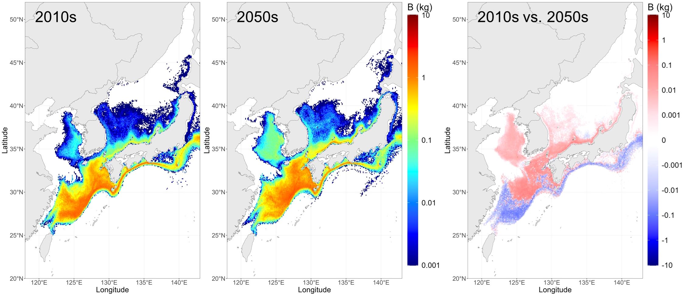
Figure 6. Biomass distribution of chub mackerel (Scomber japonicus) larvae, immediately after the completion of metamorphosis (> 1.5 cm FL), averaged between February and July for the 2010s and the 2050s, and the differences between the two periods. The unit is kilogram per 0.1°×0.1°.

Table 4

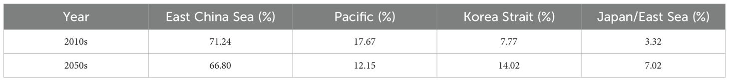
Table 4. The proportion of chub mackerel (Scomber japonicus) larval biomass immediately after the completion of metamorphosis (> 1.5 cm FL), averaged between February and July for 2010–2019 and 2050–2059 in the different areas.

In addition, the reduced influence of oceanic currents (such as the KC or the TWC) on larval dispersal may have increased the exposure of larvae to elevated water temperatures, contributing to the higher projected biomass. This interpretation is supported by the transport patterns and thermal conditions simulated by our IBM-TCM. Go et al. (2020) showed that higher water temperatures within the optimal range lead to a higher cumulative survival rate of chub mackerel during early-life stages because of their faster growth. Kamimura et al. (2015) reported an inverse correlation between larval stage duration and recruitment of chub mackerel, and a positive correlation between daily growth rates during larval and juvenile stages and recruitment. These findings and our results suggest that exploitable chub mackerel biomass and production will increase in the KS and the YS in the 2050s.

4.3 Sensitivity analyses and uncertainty

The medium-warming surrogate scenario, representing 50% of the mean projected warming under RCP 8.5, had minimal effects on larval biomass, with monthly values broadly similar to the baseline. In contrast, spatial shifts in the centroid were more evident, with maximum centroid shifts at 0.72° latitude and 0.73° longitude, occurring from May to July. Notably, higher levels of warming were associated with a more northerly distribution of larvae, indicating that while changes in biomass are relatively insensitive, the location of larval aggregations responds to the magnitude of warming. The findings suggest that the projected increase in larval biomass and its northward shift are qualitatively robust, but their magnitude is sensitive to the level of warming applied. Although this surrogate analysis does not encompass the entire range of potential climate scenarios, it provides a reasonable indication of how uncertainties in temperature forcing may influence larval projections and supports the reliability of our baseline RCP 8.5 forecasts.

Furthermore, we assessed the sensitivity of our projections to changes in the larval mortality parameter, growth coefficient, and spawning period. A variation in mortality by ±20% had a substantial impact on total larval biomass (-63% to +188%), whereas shifts in the biomass centroid remained negligible. Perturbing the temperature-dependent growth coefficient by ±20% caused moderate changes in biomass (-28% to +28%), but produced only minor centroid displacements. By contrast, shifting the mean spawning period by ±2 weeks led to notable decrement changes in biomass (-31% to -68%), together with more pronounced centroid shifts (-0.45°E to +0.62°E, -0.86°N to +0.25°N). Collectively, these findings suggest that uncertainties in biological parameters can substantially influence projected larval abundance, with mortality and spawning period exerting the strongest effects, but the spatial distribution patterns and their northward shift remain qualitatively robust.

We conducted the simulation 10 times and reported the mean results with 95% confidence intervals. This approach provides an indirect assessment of sensitivity to variability in the initial spatio-temporal distribution of eggs. Although a comprehensive sensitivity analysis was not performed, limiting the overall evaluation of model uncertainty, these findings offer a reliable indication of the potential impact of stochastic variability on larval biomass and spatial distribution.

4.4 Merits of this study

Our IBM-TCM predicted the spatio-temporal distribution of chub mackerel larvae by simulating the 3-dimensional coordinate of location, size, and abundance of each super-individual whose growth and mortality vary by the ambient temperature changes projected by the ROMS. While the modeling framework builds upon established IBM approaches, the novelty of this study lies in its first high-resolution application to the western North Pacific, enabling region-specific projections of larval biomass and distribution under climate change. Our model outcomes were generally compatible with the past and other observation and model studies in the region, or the differences were at least explainable, promising that the IBM-TCM can be extended to the juvenile or adult stages by adding the components for their behavior rules under ambient environmental changes.

In addition to its scientific merits, the outcomes of this study also provide valuable implications for fisheries management under climate change. The projected northward shift in the spawning and nursery grounds of chub mackerel suggests that critical early-life habitats may increasingly fall within higher-latitude regions such as the Korea Strait and the Yellow Sea. This spatial redistribution has the potential to alter recruitment dynamics, fishing ground productivity, and interannual variability in stock availability, thereby underscoring the need for spatially adaptive management strategies. As chub mackerel are shared among multiple countries in the western North Pacific, coordinated monitoring efforts and climate-informed transboundary governance will be essential to ensure sustainable resource management under changing oceanographic conditions. For each country in the region, we expect that national fisheries policies will consider and reflect the spatio-temporal shifts of chub mackerel larvae projected by the present study, modifying the relevant fisheries regulations on fishing areas and seasons.

4.5 Limitations, problems of the present study and future studies

The limitations of the present study need to be acknowledged and addressed in the future. First, our physical model was not explicitly bias-corrected and showed limited agreement with observations at fine spatial and temporal scales (Go et al., 2025). However, as shown in Appendix A, the model successfully reproduced the seasonal and vertical temperature structure based on observed oceanographic data from KODC. Although Appendix A indicates no significant differences in warming trends between KODC observations and ROMS outputs, we note that slope comparisons with small sample sizes do not fully capture potential biases or the spatial structure of surface temperature fields within the model domain. While large-scale patterns were broadly realistic, future improvements using data assimilation techniques or sea temperature bias correction are recommended to enhance spatial accuracy and increase confidence in the biological projections.

Second, the projected larval distribution and biomass from our IBM-TCM were partially validated against observed data, providing only a limited assessment of reliability. Although the Pearson correlation offered a quantitative indication of spatial match, this single metric cannot fully capture mismatches in timing, magnitude, or extent. To improve the model performance, international collaborative research among countries in the region is recommended, particularly conducting comprehensive ichthyoplankton surveys in the western North Pacific and sharing fisheries data.

Third, we exclusively relied on a single climate projection, the RCP 8.5 scenario from AR5. While RCP 8.5 remains useful for exploring worst-case outcomes, future studies should incorporate multiple pathways from updated climate change scenarios (e.g., SSP2-4.5, SSP5-8.5 of AR6) to better reflect a range of plausible climate futures, represent environmental uncertainty, and improve the policy relevance of the projections.

Fourth, a caveat is made regarding the definition of the present-day climatological baseline. While 30-year averaging period is generally recommended in climatology to account for interannual variability, this study used a shorter 10-year period (2010–2019) as a proxy for present-day conditions due to computational and data constraints. Although this shorter baseline captures recent climate states relevant to the spawning and early development of chub mackerel, it may not fully represent long-term natural variability. As such, the projected changes should be interpreted with caution, and future studies incorporating extended climatological baselines are needed to validate and refine these results.

Fifth, a limitation of the present model is the exclusion of active behavioral components such as diel vertical migration. Although passive vertical movement was estimated daily based on physical processes (e.g., vertical advection and buoyancy), the lack of behaviorally regulated depth preferences may affect the accuracy of larval temperature exposure and dispersal pathways. Incorporating behavior-based vertical migration into future models could improve the accuracy of larval transport and survival estimations.

Lastly, although we considered only water temperature, the growth and survival of chub mackerel larvae can be influenced by other factors such as food availability. Taga et al. (2019) suggested that temperature and prey density impact the growth rate of chub mackerel larvae, and Li et al. (2012) took a growth and mortality model based on water temperature and food availability to simulate an IBM for chub mackerel larvae. Therefore, it is necessary to develop and enhance the growth and mortality functions based on these additional factors to improve the model performance once the relevant data are available.

5 Conclusion

We developed a bio-physical coupling IBM for Tsushima Warm Current stock of chub mackerel during early-life stages in the western North Pacific. Despite uncertainties, our IBM-TCM projected that the increased regional water temperature, including spawning ground, due to global warming will increase the overall larval chub mackerel biomass by the 2050s and shift their distribution northward. This is the first case study in projecting spatio-temporal changes of chub mackerel at high-resolution by developing and applying an IBM based on a Lagrangian particle tracking method in the western North Pacific, providing region-specific insights to support adaptive fisheries management under climate change.

For fisheries management and adaptation to climate change, it is more urgent to project the movement and distribution of the post-recruit juveniles and adults. Our model is limited in predicting spatio-temporal changes in the biomass of juvenile and adult mackerel driven by climate change, because it was developed for the pre-recruit early-life stages. For a comprehensive understanding of how climate change may affect the full life cycle of chub mackerel, future improvements to the model may include incorporating additional ecological processes, such as prey availability, predation, and post-metamorphic movement and survival, to enhance predictive accuracy. We plan to consider the entire life stages in our extended version of IBM to project the spatio-temporal changes of exploitable chub mackerel in the region.

We expect that our presented study will enhance the reliability of stock assessment for fisheries management of chub mackerel and contribute to developing fisheries policy and management plan for adaptation to climate change in the region.

Data availability statement

The original contributions presented in the study are included in the article/Supplementary Material. Further inquiries can be directed to the corresponding author/s.

Author contributions

SG: Conceptualization, Investigation, Visualization, Software, Data curation, Validation, Funding acquisition, Writing – review & editing, Methodology, Formal analysis, Writing – original draft. SJ: Conceptualization, Methodology, Writing – review & editing, Supervision, Resources, Software, Funding acquisition, Project administration.

Funding

The author(s) declare financial support was received for the research and/or publication of this article. This research was supported by the Korea Institute of Marine Science and Technology (KIMST) funded by the Ministry of Oceans and Fisheries (RS-2023-00256330 and RS-2024-00406249).

Conflict of interest

The authors declare that the research was conducted in the absence of any commercial or financial relationships that could be construed as a potential conflict of interest.

Generative AI statement

The author(s) declare that no Generative AI was used in the creation of this manuscript.

Any alternative text (alt text) provided alongside figures in this article has been generated by Frontiers with the support of artificial intelligence and reasonable efforts have been made to ensure accuracy, including review by the authors wherever possible. If you identify any issues, please contact us.

Publisher’s note

All claims expressed in this article are solely those of the authors and do not necessarily represent those of their affiliated organizations, or those of the publisher, the editors and the reviewers. Any product that may be evaluated in this article, or claim that may be made by its manufacturer, is not guaranteed or endorsed by the publisher.

Supplementary material

The Supplementary Material for this article can be found online at: https://www.frontiersin.org/articles/10.3389/fmars.2025.1648650/full#supplementary-material

References

Blaxter J. H. S. (1992). The effect of temperature on larval fishes. Neth. J. Zool. 42, 336–357. doi: 10.1163/156854291X00379

Crossref Full Text | Google Scholar

Brochier T., Colas F., Lett C., Echevin V., Cubillos L. A., Tam J., et al. (2009). Small pelagic fish reproductive strategies in upwelling systems: A natal homing evolutionary model to study environmental constraints. Prog. Oceanogr. 83, 261–269. doi: 10.1016/j.pocean.2009.07.044

Crossref Full Text | Google Scholar

Cha H. K., Choi Y. M., Park J. H., Kim J. Y., and Sohn M. H. (2002). Maturation and spawning of the chub mackerel, Scomber japonicus Houttuyn in Korean waters. J. Korean Soc Fish. Res. 5, 24–33.

Google Scholar

Chang Y.-L., Sheng J., Ohashi K., Béguer-Pon M., and Miyazawa Y. (2015). Impacts of interannual ocean circulation variability on Japanese eel larval migration in the western North Pacific Ocean. PloS One 10, e0144423. doi: 10.1371/journal.pone.0144423, PMID: 26642318

PubMed Abstract | Crossref Full Text | Google Scholar

Choi Y. M., Park J. H., Cha H. K., and Hwang K. S. (2000). Age and growth of common mackerel, Scomber japonicus Houttuyn, in Korean waters. J. Korean Soc Fish. Res. 3, 1–8.

Google Scholar

Christensen A., Daewel U., Jensen H., Mosegaard H., John M. S., and Schrum C. (2007). Hydrodynamic backtracking of fish larvae by individual-based modelling. Mar. Ecol. Prog. Ser. 347, 221–232. doi: 10.3354/meps06980

Crossref Full Text | Google Scholar

Deangelis D. L., Godbout L., and Shuter B. J. (1991). An individual-based approach to predicting density-dependent dynamics in smallmouth bass populations. Ecol. Model. 57, 91–115. doi: 10.1016/0304-3800(91)90056-7

Crossref Full Text | Google Scholar

Deangelis D. L. and Grimm V. (2014). Individual-based models in ecology after four decades. F1000Prime Rep. 6, 39. doi: 10.12703/P6-39, PMID: 24991416

PubMed Abstract | Crossref Full Text | Google Scholar

Fritzsche R. A. (1978). Development of fishes of the mid-Atlantic Bight: An Atlas of egg, larval, and juvenile stages, Vol. 5 Chaetodontidae through Ophidiidae (Maryland: Fish and Wildlife Service, U.S. Department of the Interior).

Google Scholar

Gilbert C. S., Gentleman W. C., Johnson C. L., Dibacco C., Pringle J. M., and Chen C. (2010). Modelling dispersal of sea scallop (Placopecten magellanicus) larvae on Georges Bank: the influence of depth-distribution, planktonic duration and spawning seasonality. Prog. Oceanogr. 87, 37–48. doi: 10.1016/j.pocean.2010.09.021

Crossref Full Text | Google Scholar

Go S. and Jung S. (2023). Estimation of size-dependent mortality of chub mackerel (Scomber japonicus) based on their fecundity. Ocean Sci. J. 58, 19. doi: 10.1007/s12601-023-00113-2

Crossref Full Text | Google Scholar

Go S., Lee K., and Jung S. (2020). A temperature-dependent growth equation for larval chub mackerel (Scomber japonicus). Ocean Sci. J. 55, 157–164. doi: 10.1007/s12601-020-0004-z

Crossref Full Text | Google Scholar

Go S., Lee J.-H., and Jung S. (2025). Projecting the shift of chub mackerel (Scomber japonicus) spawning grounds driven by climate change in the western North Pacific ocean. Fishes 10, 20. doi: 10.3390/fishes10010020

Crossref Full Text | Google Scholar

Guan W., Ma X., He W., and Cao R. (2023). Simulation of the distribution, growth, and survival rate of chub mackerel larvae and juveniles in the East China Sea. J. Oceanology Limnology 41, 1602–1619. doi: 10.1007/s00343-022-2012-6

Crossref Full Text | Google Scholar

Guo C., Ito S.-I., Kamimura Y., and Xiu P. (2022). Evaluating the influence of environmental factors on the early life history growth of chub mackerel (Scomber japonicus) using a growth and migration model. Prog. Oceanogr. 206, 102821. doi: 10.1016/j.pocean.2022.102821

Crossref Full Text | Google Scholar

He W., Guan W., and Cao R. (2024). Dynamic energy budget model for the complete life cycle of chub mackerel in the Northwest Pacific. Fish. Res. 270, 106902. doi: 10.1016/j.fishres.2023.106902

Crossref Full Text | Google Scholar

Hinckley S., Hermann A. J., and Megrey B. A. (1996). Development of a spatially explicit, individual-based model of marine fish early life history. Mar. Ecol. Prog. Ser. 139, 47–68. doi: 10.3354/meps139047

Crossref Full Text | Google Scholar

Hiyama Y., Yoda M., and Ohshimo S. (2002). Stock size fluctuations in chub mackerel (Scomber japonicus) in the East China Sea and the Japan/East Sea. Fish. Oceanogr. 11, 347–353. doi: 10.1046/j.1365-2419.2002.00217.x

Crossref Full Text | Google Scholar

Houde E. D. (1987). Fish early life dynamics and recruitment variability. Am. Fish. Soc Symp. 2, 17–29.

Google Scholar

Houde E. D. (2009). “Recruitment Variability,” in Fish Reproductive Biology: Implications for Assessment and Management, 1st ed. Eds. Jakobsen T., Fogarty M. J., Megrey B. A., and Moksness E. (John Wiley & Sons, West Sussex), 91–171.

Google Scholar

Hunter J. R. and Kimbrell C. A. (1980). Early life history of Pacific mackerel, Scomber japonicus. Fish. Bull. 78, 89–101.

Google Scholar

Huston M., Deangelis D., and Post W. (1988). New computer models unify ecological theory: computer simulations show that many ecological patterns can be explained by interactions among individual organisms. Biosci. 38, 682–691. doi: 10.2307/1310870

Crossref Full Text | Google Scholar

Hwang K. and Jung S. (2012). Decadal changes in fish assemblages in waters near the Ieodo ocean research station (East China Sea) in relation to climate change from 1984 to 2010. Ocean Sci. J. 47, 83–94. doi: 10.1007/s12601-012-0009-3

Crossref Full Text | Google Scholar

Hwang S.-D., Kim J.-Y., and Lee T.-W. (2008). Age, growth, and maturity of chub mackerel off Korea. N. Am. J. Fish. Manage 28, 1414–1425. doi: 10.1577/M07-063.1

Crossref Full Text | Google Scholar

IPCC (2014). Climate change 2014: Impacts, adaptation and vulnerability. Part B: Regional aspects. Contribution of working group II to the fifth assessment report of the intergovernmental panel on climate change (Cambridge, United Kingdom and New York, NY, USA: Cambridge University Press).

Google Scholar

Jung M. K. (1977). The fishes of Korea (Seoul: Iljisa).

Google Scholar

Jung S. (2008). Spatial variability in long-term changes of climate and oceanographic conditions in Korea. J. Environ. Biol. 29, 519–529., PMID: 19195391

PubMed Abstract | Google Scholar

Jung S., Ha S., and Na H. (2013). Multi-decadal changes in fish communities Jeju Island in relation to climate change. Korean J. Fish. Aquat. Sci. 46, 186–194. doi: 10.5657/KFAS.2013.0186

Crossref Full Text | Google Scholar

Jung S., Pang I.-C., Lee J.-H., Choi I., and Cha H. K. (2014). Latitudinal shifts in the distribution of exploited fishes in Korean waters during the last 30 years: a consequence of climate change. Rev. Fish. Biol. Fish. 24, 443–462. doi: 10.1007/s11160-013-9310-1

Crossref Full Text | Google Scholar

Jung S., Pang I.-C., Lee J.-H., and Lee K. (2016). Climate-change driven range shifts of anchovy biomass projected by bio-physical coupling individual based model in the marginal seas of East Asia. Ocean Sci. J. 51, 563–580. doi: 10.1007/s12601-016-0055-3

Crossref Full Text | Google Scholar

Kamimura Y., Takahashi M., Yamashita N., Watanabe C., and Kawabata A. (2015). Larval and juvenile growth of chub mackerel Scomber japonicus in relation to recruitment in the western North Pacific. Fish. Sci. 81, 505–513. doi: 10.1007/s12562-015-0869-4

Crossref Full Text | Google Scholar

Kim S. R., Kim J. J., Stockhausen W. T., Kim C.-S., Kang S., Cha H. K., et al. (2019). Characteristics of the eggs and larval distribution and transport process in the early life stage of the chub mackerel Scomber japonicus near Korean waters. Korean J. Fish. Aquat. Sci. 52, 666–684. doi: 10.5657/KFAS.2019.0666

Crossref Full Text | Google Scholar

Kramer D. (1960). Development of eggs and larvae of Pacific mackerel and distribution and abundance of larvae 1952–1956. Fish. 60, 393–438.

Google Scholar

Lee K., Go S., and Jung S. (2021). Long-term changes in fish assemblage structure in the Korea Strait from 1986 to 2010 in relation with climate change. Ocean Sci. J. 56, 182–197. doi: 10.1007/s12601-021-00016-0

Crossref Full Text | Google Scholar

Lee H. H., Kang S., Jung K.-M., Jung S., Sohn D., and Kim S. (2017). Observed pattern of diel variation in specific gravity of Pacific mackerel eggs and larvae. Ocean Polar Res. 39, 257–267. doi: 10.4217/OPR.2017.39.4.257

Crossref Full Text | Google Scholar

Lee S.-J., Kim J.-B., and Han S.-H. (2016). Distribution of mackerel, Scomber japonicus eggs and larvae in the coast of Jeju Island, Korea in spring. J. Korean Soc Fish. Ocean Technol. 52, 121–129. doi: 10.3796/KSFT.2016.52.2.121

Crossref Full Text | Google Scholar

Letcher B. H., Rice J. A., Crowder L. B., and Rose K. A. (1996). Variability in survival of larval fish: disentangling components with a generalized individual-based model. Can. J. Fish. Aquat. Sci. 53, 787–801. doi: 10.1139/f95-241

Crossref Full Text | Google Scholar

Li Y., Chen X., Chen C., Ge J., Ji R., Tian R., et al. (2014a). Dispersal and survival of chub mackerel (Scomber japonicus) larvae in the East China Sea. Ecol. Model. 283, 70–84. doi: 10.1016/j.ecolmodel.2014.03.016

Crossref Full Text | Google Scholar

Li Y., Chen X., and Yang H. (2012). Construction of individual-based ecological model for Scomber japonicas at its early growth stages in East China Sea. Chin. J. Appl. Ecol. 23, 1695–1703., PMID: 22937663

PubMed Abstract | Google Scholar

Li Y., Pan L., and Chen X. (2014b). Effect of spawning ground location on the transport and growth of chub mackerel (Scomber japonicus) eggs and larvae in the East China Sea. Acta Ecol. Sin. 34, 92–97. doi: 10.1016/j.chnaes.2013.06.001

Crossref Full Text | Google Scholar

Massicotte P., South A., and Hufkens K. (2023). rnaturalearth: World map data from natural earth. R package version 1.0.1. Available online at: https://cran.r-project.org/package=rnaturalearth (Accessed June 10, 2025).

Google Scholar

Megrey B. A. and Hinckley S. (2001). Effect of turbulence on feeding of larval fishes: a sensitivity analysis using an individual-based model. ICES J. Mar. Sci. 58, 1015–1029. doi: 10.1006/jmsc.2001

Crossref Full Text | Google Scholar

Mendiola D., Alvarez P., Cotano U., and Martínezde Murguía A. (2007). Early development and growth of the laboratory reared north-east Atlantic mackerel Scomber scombrus L. J. Fish Biol. 70, 911–933. doi: 10.1111/j.1095-8649.2007.01355.x

Crossref Full Text | Google Scholar

Norcross B. L. and Shaw R. F. (1984). Oceanic and estuarine transport of fish eggs and larvae: a review. Trans. Am. Fish. Soc 113, 153–165. doi: 10.1577/1548-8659(1984)113<153:OAETOF>2.0.CO;2

Crossref Full Text | Google Scholar

Okunishi T., Yamanaka Y., and Ito S.-I. (2009). A simulation model for Japanese sardine (Sardinops melanostictus) migrations in the western North Pacific. Ecol. Model. 220, 462–479. doi: 10.1016/j.ecolmodel.2008.10.020

Crossref Full Text | Google Scholar

Parada C., van der Lingen C. D., Mullon C., and Penven P. (2003). Modelling the effect of buoyancy on the transport of anchovy (Engraulis capensis) eggs from spawning to nursery grounds in the southern Benguela: an IBM approach. Fish. Oceanogr. 12, 170–184. doi: 10.1046/j.1365-2419.2003.00235.x

Crossref Full Text | Google Scholar

R Core Team (2024). R: A language and environment for statistical computing (Vienna: R Foundation for Statistical Computing). Available online at: https://www.R-project.org.

Google Scholar

Sassa C. and Tsukamoto Y. (2010). Distribution and growth of Scomber japonicus and S. australasicus larvae in the southern East China Sea in response to oceanographic conditions. Mar. Ecol. Prog. Ser. 419, 185–199. doi: 10.3354/meps08832

Crossref Full Text | Google Scholar

Scheffer M., Baveco J., Deangelis D., Rose K. A., and Van Nes E. (1995). Super-individuals a simple solution for modelling large populations on an individual basis. Ecol. Model. 80, 161–170. doi: 10.1016/0304-3800(94)00055-M

Crossref Full Text | Google Scholar

Taga M., Kamimura Y., and Yamashita Y. (2019). Effects of water temperature and prey density on recent growth of chub mackerel Scomber japonicus larvae and juveniles along the Pacific coast of Boso–Kashimanada. Fish. Sci. 85, 931–942. doi: 10.1007/s12562-019-01354-8

Crossref Full Text | Google Scholar

Van Winkle W., Rose K. A., and Chambers R. C. (1993). Individual-based approach to fish population dynamics: an overview. Trans. Am. Fish. Soc 122, 397–403. doi: 10.1577/1548-8659(1993)122<0397:IBATFP>2.3.CO;2

Crossref Full Text | Google Scholar

Wang Z., Ito S.-I., Yabe I., and Guo C. (2023). Development of a bioenergetics and population dynamics coupled model: A case study of chub mackerel. Front. Mar. Sci. 10. doi: 10.3389/fmars.2023.1142899

Crossref Full Text | Google Scholar

Watanabe C., Yatsu A., and Watanabe Y. (2002). Changes in growth with fluctuation of chub mackerel abundance in the Pacific waters off central Japan from 1970 to 1997 (Sidney, B.C., Canada: PICES-GLOBEC International Program on Climate Change and Carrying Capacity).

Google Scholar

Werner F. E., Quinlan J. A., Lough R. G., and Lynch D. R. (2001). Spatially-explicit individual based modeling of marine populations: a review of the advances in the 1990s. Sarsia 86, 411–421. doi: 10.1080/00364827.2001.10420483

Crossref Full Text | Google Scholar

Wickham H. (2016). ggplot2: Elegant graphics for data analysis (New York: Springer-Verlag). doi: 10.1007/978-3-319-24277-4

Crossref Full Text | Google Scholar

Yamada U., Tokimura M., Horikawa H., and Nakabo T. (2007). Fishes and fisheries of the East China and Yellow Seas (Tokyo, Japan: Tokai University press).

Google Scholar

Yukami R., Ohshimo S., Yoda M., and Hiyama Y. (2009). Estimation of the spawning grounds of chub mackerel Scomber japonicus and spotted mackerel Scomber australasicus in the East China Sea based on catch statistics and biometric data. Fish. Sci. 75, 167–174. doi: 10.1007/s12562-008-0015-7

Crossref Full Text | Google Scholar

Appendix A

We evaluated whether the regional ocean circulation model (ROMS) reproduced the long-term trends of water temperature observed in the Korea Oceanographic Data Center (KODC) dataset from 2010 to 2019. For each depth (0–75 m), we calculated linear regression slopes of bimonthly averaged water temperatures for both observed and model-predicted values. To compare these slopes, we conducted Student’s t-tests to determine whether the ROMS and observed data showed statistically different temporal trends. The results (Table A1) showed no significant difference (p > 0.05) in slope between observed and ROMS-predicted temperatures at all depths. These findings indicate that the ROMS reliably captured the interannual warming trend in the upper 75 m of the study area.

Table A1

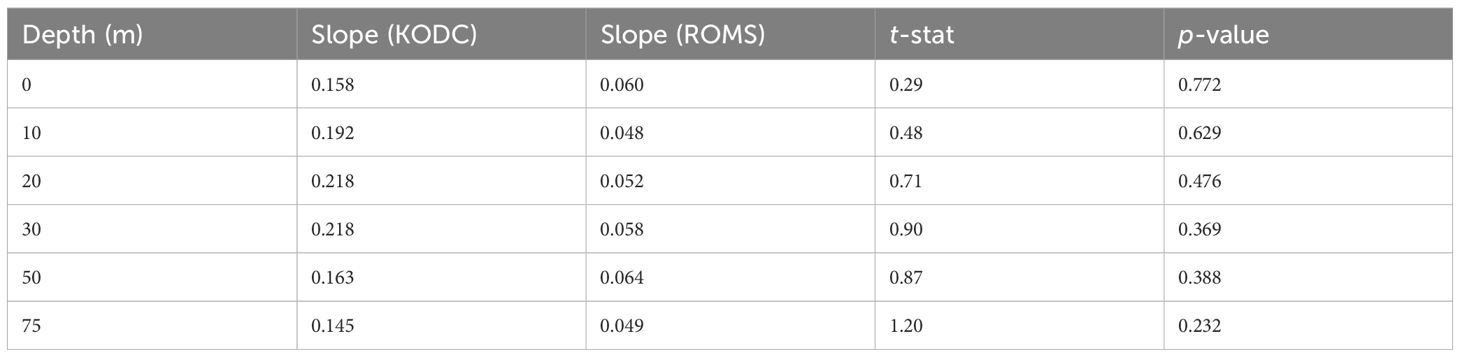
Table A1. Results of Student’s t-tests comparing the slopes of linear regression for bimonthly averaged water temperatures between observed (Korea Ocean Data Center; KODC) and modeled (regional ocean circulation model; ROMS) data for the 2010s (2010–2019).

In addition, we evaluated the model’s ability to reproduce the absolute magnitude of sea surface temperatures from February to June by calculating bias (model - observation) and root mean square error (RMSE) against in-situ KODC measurements. The results (Table A2) indicated relatively minor mean biases ranging from -0.28 to +1.53°C and RMSE values below 2.73°C across the ECS, KS/YS, and ES, based on 5,637 station observations. No in-situ data were available for the Pacific Ocean (PO). These statistics further support the robustness of the ROMS forcing fields used in our bio-physical coupled simulations.

Table A2

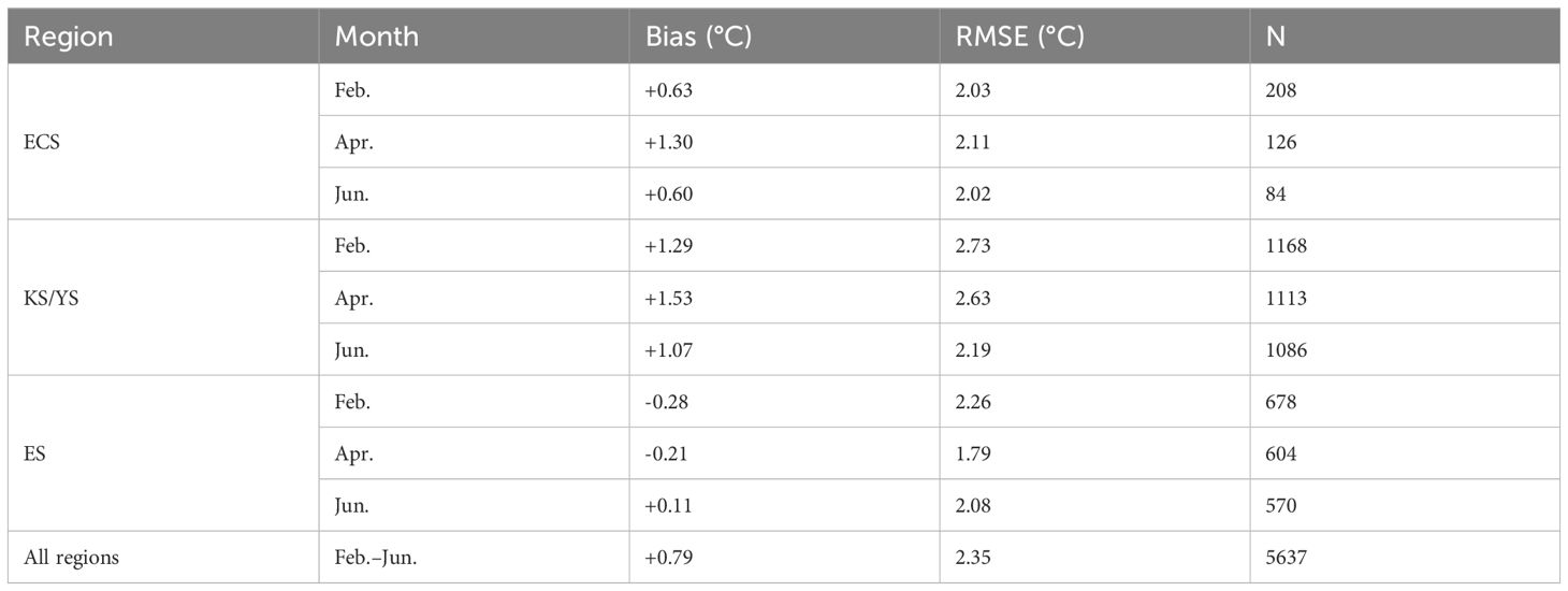
Table A2. Bias and RMSE of modeled surface temperature compared with in-situ observations (Korea Ocean Data Center; KODC) for February–June in the East China Sea (ECS), Korea Strait/Yellow Sea (KS/YS), and Japan/East Sea (ES) during the 2010s (2010–2019). No data were available for the Pacific Ocean (PO).

Appendix B

To evaluate the influence of viscosity on the estimated terminal velocity, we compared results using the physical kinematic viscosity of seawater (= 1 × 10⁻⁶ m²/s) with those obtained using the effective viscosity (= 0.01 m²/s) originally applied by Parada et al. (2003) (Table B1). The physical viscosity produces vertical velocities that would rapidly move eggs and larvae, inconsistent with field observations of their residence in the surface layer. In contrast, the effective viscosity provides a more realistic representation of biological drag effects, such as non-spherical morphology, surface mucus, and micro-scale turbulence. We also calculated the Reynolds number (Re = v_sR_l/ν or Re = v_s·2R_s/ν), which measures the ratio of inertial to viscous forces. The validity of Stokes′ law is determined by the Re value, with Re < 0.5 generally indicating that viscous forces dominate. Our estimates show that with physical viscosity, Re can exceed 10⁶ for eggs and larvae, clearly violating Stokes conditions, whereas with effective viscosity Re remains < 1 for eggs and small larvae and ≈ 0.35–0.37 for large larvae, ensuring the regime assumption is satisfied.

Table B1

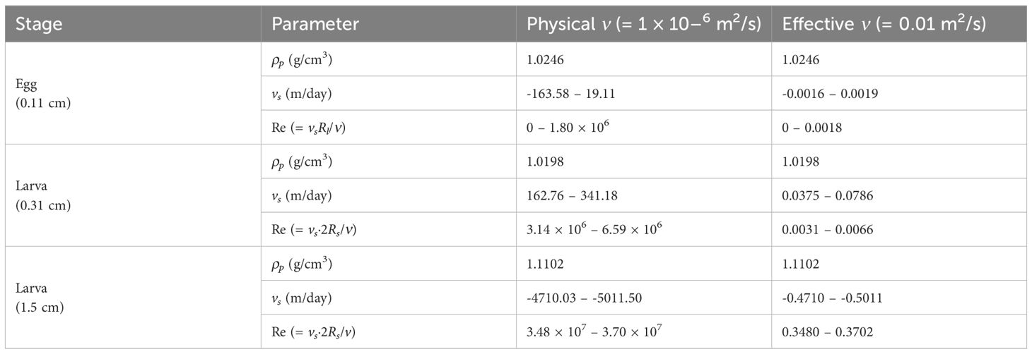
Table B1. Estimated sinking velocities (v_s, m/day) and Reynolds numbers (Re) of chub mackerel (Scomber japonicus) eggs and larvae in May 2014, using seawater density values (1.0241–1.0289 g/cm³) reported by Lee et al. (2017). ρ_p is the specific density of chub mackerel (g/cm³), and positive v_s indicates sinking whereas negative v_s indicates rising.