Learning Causal Effects From Observational Data in Healthcare: A Review and Summary

Introduction

In healthcare, it is important to distinguish between association and causation when we study treatment effects on patient outcomes. Association between two variables is non-directional and implies that the two variables are correlated. In contrast, causation is directional and indicates that one variable causes the other. In clinical studies, we are more interested in causal analysis to reveal whether a treatment causes a desired outcome.

Using observational data to infer causal treatment effects has become popular in the past decade due to two pivotal advances: the increasingly available patient data captured in Electronic Health Records (EHRs) and machine learning techniques that can efficiently and intelligently analyze large-scale data. On the data side, health care providers worldwide have widely adopted EHRs (1, 2), which capture patients' clinical and demographic information during interactions with health systems. In addition to EHRs, patient claims data are increasingly available to improve models in the healthcare domain (3). On the algorithm side, machine learning models such as artificial neural networks are powering online search engines, shopping websites, and recommender systems (4). These machine learning models are increasingly used to improve causal inference algorithms.

In the past, many different schools of learning causality coming from different fields of statistics resulted a fractured state of causal inference, creating confusion about which algorithm to use in a study. Recently, the intersection of causal inference, machine learning, and patient data has formed a new front in clinical research. Accordingly, many traditional causal inference models have been improved and many new models have been proposed. While this has enhanced the number of model options to select from in causal inference studies, it has also led to even greater confusion about which type of algorithm is appropriate for a given application. Lack of systematic knowledge of which approaches are promising in theory vs. the approaches that have been validated through real world applications further complicates the debate.

There are different stakeholders in healthcare, including healthcare providers, administrators, clinical researchers, data scientists, and many others. While data scientists, computer engineers, and biomedical statisticians may be less prone to such confusion, the fractured state in this field makes it difficult for other participants to understand the many different types of models and intuitively interpret the model results. We believe it is imperative to address this confusion for all healthcare participants to unlock the massive potential to improve patient outcomes that could be obtained by studying the causal effects of interventions from large-scale, representative, observational patient data that is now available.

In this review, we start by explaining the broad and heterogenous fields of causal inference. We then distill all of these techniques down into a simple unified framework of three algorithm families, based on size of the target patient population that the causal effect estimation will be applied to. This simple unified frame based on the size of the target patient population is important: while statisticians in medical informatics may not necessarily group the algorithms this way, it is beneficial for frontline healthcare professionals such as doctors and nurses to understand the drug effect in the context of its target population, and the effect's variance and bias characteristics when the drug is applied to the treated patient. From the perspective of this unified framework, we then review all existing applications of causal inference in healthcare in the literature, and identify key components of causal inference that are, as of now, lacking in the healthcare domain. Finally, we use these insights to create an intuitive schematic to guide researchers and stakeholders through the process of selecting an appropriate causal inference technique based on their study objectives.

This review is an extension of several works in previous literature on observational causal inference. For example, the authors in Yao et al. (5), Guo et al. (6), and Ding and Li (7) reviewed causal inference in general but without a focus on clinical settings. The authors in Landsittel et al. (8) offered a narrative review of basic concepts of causal inference but did not consider new developments in this field. Prior reviews (9–11) have narrowly focused on the matching method of causal inference, while in this paper we expand to include a much broader algorithm types.

We conclude this section by providing below a summary of all the approaches we review, with respect to their variance-bias trade-off, advantages, disadvantages, and how widely they are applied in clinical studies.

Causal Inference Assumptions, Frameworks, and Target-Population Intervention Sizes

Confounding Variables

Causal inference differs from associative studies due to the modeling of confounding variables (covariates), defined as variables that affect both the treatment and the outcome. In associative studies which focus on patient outcome estimates, confounding variables are modeled in an inclusive manner because the inclusion of these variables in the model improves estimate accuracy. In contrast, causal inference which reveals the causal relationship between treatments and patient outcomes models the confounding variables in an exclusive manner in that their effects are removed through various approaches we review in this paper.

Assumptions

In the literature, several assumptions are widely adopted in causal inference (12). The unconfoundedness assumption, also known as ignorability, states that all confounding variables are observed in the data. In practice, domain experts often examine as many patient variables as possible, including their demographic and clinical characteristics, so that this assumption can be met. The common support or positivity assumption states that any patient has a non-zero probability of being present in any of the treatment groups. The validity of this assumption can be checked by calculating the patients' propensity scores (12). The Stable Unit Treatment Value assumption (SUTVA) states that a patient's outcome only depends on the treatment this patient receives, and not affected by the outcome or treatment of any other patients. The consistency assumption links the potential outcomes to the observed data and implies that the potential outcome under an observed exposure is precisely the outcome that is observed (13).

Bias-Variance Tradeoffs Based on Target-Population Intervention Sizes

Researchers, clinicians, and other healthcare stakeholders may wish to know the treatment effects at different population levels for different purposes. For example, they may want to evaluate the overall effectiveness of the treatment on the whole population. They may want to understand treatment effect differences in different subpopulations to identify the subpopulation where the treatment is the most effective or least effective. When they treat an individual patient, they may want to know the individual-level treatment effects considering the patient's unique medical benefits and risks.

Driven by such needs, researchers conduct causal inference at different target-population intervention sizes: at one end of the spectrum is the Average Treatment Effect (ATE) that captures the treatment effect for a population at large; at the other end is the Individual Treatment Effect (ITE) that captures the treatment effect heterogeneity across individuals; in between is the conditional average treatment effect (CATE) that captures the treatment effect for subpopulations.

In clinical practices, at the receiving end of any treatment are individual patients. Correspondingly, different treatment effects (ATE, CATE, and ITE) are eventually applied to individual patients. Therefore, it is important to understand the variance-bias tradeoff of the estimate at different target-population intervention sizes: if we use ATE as the treatment effect for an individual patient, the bias will be high due to effect heterogeneity across patients in the population, but the variance will be low due to more data being used in the inference; in contrast, if we use ITE for a patient, the bias will be low, but the variance will be high.

As the rest of the paper shows, ATE provides the best option and fosters estimate efficiency for the whole population, but may not provide the most accurate estimate for any individual patient. ITE maximally leverages the data, but risks being uninterpretable to clinical practitioners. CATE represents a balance between bias and variance and tracks the clinical definition of patient subgroups.

Two Frameworks

There are two widely accepted frameworks in the literature for causal inference: the structural causal model (SCM) (14–16) and the potential outcome framework (POF) (12, 17, 18). SCM consists of two components, the causal graph and the structural equations. A causal graph is a directed acyclic graph (DAG) where the edges represent causal relationships, and the nodes represent variables including treatments, outcomes, and covariates that may or may not be observed. Causal effects can be quantitatively specified through a set of structural equations.

The DAG and structural equations together provide a comprehensive theory of causality and seamlessly tie essential concepts and methodologies in causal inference (14, 19, 20). In addition, it can possibly deal with cases where confounders cannot be measured. For example, in Barter (21), the author used the blood type as an instrument variable—defined as a variable that affects the outcome only through the treatment variable—to estimate the average survival benefit from receiving a liver transplant.

The other framework, called the potential outcome framework, centers on the concept of potential outcomes. In the simplest term, potential outcomes are all the possible outcomes for a patient under all possible treatments, with each outcome corresponding to a treatment. Note that only one potential outcome can be observed for a given patient at a given time. We call the potential outcome that would have been observed had the treatment been different the counterfactual or the missing outcome. In the simplest case, there is only one treatment to consider. A patient can be either given the treatment, i.e., assigned to the treated group, or given no treatment, i.e., assigned to the control group. Under the potential outcome framework, the treatment effect is the difference between the potential outcome if the patient is treated and that if the patient is not treated.

CSM and POF are not competing frameworks but can be unified (22). Despite this fact, the two frameworks have differences in what causal questions they are best suited to handle. Given its strong theoretical grounding, CSM is ideally suited to identifying unknown causal and confounding variables, as well as facilitating explanation. While it is useful to identify all the variables in the causal graph and their causal connections, the primary objective in healthcare is often to estimate the actual effect of a given treatment. POF is best suited for generating these estimates, because comparing potential outcomes eases the removal of confounding effects and enables a natural connection to traditional statistical analyses. For this reason, POF is more widely adopted for healthcare research and will be the focus of this review.

Causal Inference Methods by Target-Population Intervention Sizes

In this section we review causal inference approaches in the literature under the potential outcome framework and the assumptions stated in Section Causal Inference Assumptions, Frameworks, and Target-Population Intervention Sizes. We organize our review by the approaches' target-population intervention size: from ATE for the whole population to CATE for subpopulations and ITE for individual patients.

We first explain some key notations. Suppose we are interested in the causal effect of a treatment A on outcome Y. The potential outcome denoted by Y^a is the outcome that we would observe under a possible treatment A = a. In a binary treatment case, a can possibly take on two values a∈{0, 1}, where 0 indicates the patient is not treated and 1 indicates the patient is treated. We denote the confounding variables by X. For simplicity, we only focus on the binary treatment case in this paper.

Estimate ATE for the Whole Population

In the binary treatment case, the ATE estimate for the population can be calculated as

$\begin{array}{ll}\tau =E\left(Y^1-Y^0\right)=E\left(Y^1\right)-E\left(Y^0\right)& (1)\end{array}$

It is the difference between the expected potential outcomes of the population if everyone is treated (A = 1) and if no one is treated (A = 0).

Note that ATE cannot be directly calculated from equation (1) because only one of the potential outcomes, either $Y_i^1$or $Y_i^0$, can be directly observed for patient i, nor can it be directly calculated from the expected outcomes of the treated and control groups,

$\begin{array}{ll}E\left(Y^1-Y^0\right)\ne E(Y|A=1)-E(Y|A=0)& (2)\end{array}$

due to the existence of confounding variables X. In general, the distribution of confounding variables is different in the treated and control group. If their expected outcomes are directly compared to calculate treatment effects without adjusting for confounding variables, the calculated treatment effects would be biased.

Propensity Score-Based Approaches

Propensity score of a patient is the conditional probability that this patient with X = x is assigned to the treated group. It is expressed as

$\begin{array}{l}\pi (x)=P_r(A=1|X=x),\end{array}$

and can be estimated using models such as logistic regression (12). We can use the propensity score in three different ways to balance the covariate distribution between the treated and control group and thus make the two groups comparable.

The first way is to create new control and treated groups using propensity score matching (12, 23). The most straightforward approach is greedy one-to-one matching: one patient from the control group is matched to one patient from the treated group based on their propensity scores. Data of unmatched patients gets thrown away. The covariate distribution of the matched control and treated group is balanced. Then we can calculate the difference of the expected outcomes of the two new groups as the average treatment effect (ATE). In contrast to equation (2), the equation below is now correct due to balanced covariate distributions,

$\begin{array}{l}{E\left(Y^1-Y^0\right)}_{balanced}={E(Y|A=1)}_{balanced}-{E(Y|A=0)}_{balanced}\end{array}$

In addition to one-to-one matching, propensity score is used in other similar algorithms to create matched groups. These algorithms differ from each other in whether patients are chosen with or without replacement (24), whether matching is optimal, greedy (24), one-to-one, or one-to-many (25), and what metric is used to measure similarity between two patients (11, 23, 26, 27).

The second way of using propensity scores, known as Inverse Probability of Treatment Weighting (IPTW) (28), is to assign different patients with different weights in the calculation of ATE. For patient i, the weight is calculated as

$\begin{array}{l}{w}_i=\frac{A_i}{P(A_i=1|X_i)}+\frac{1-A_i}{1-P(A_i=1|X_i)}.\end{array}$

From this equation, we can see that if patient i is in the treated group (A_i = 1), the weight assigned to this patient is $w_i=\frac{1}{P(A_i=1|X_i)}=\frac{1}{\pi (x_i)}$. If the patient i is in the control group (A_i = 0), the weight then becomes $w_i=\frac{1}{1-P(A_i=1|X_i)}=\frac{1}{1-\pi (x_i)}$. The weight of a patient in a group is just the inverse probability of this patient being assigned to this group. The ATE of the population can then be calculated as

$\begin{array}{l}\widehat{\tau }=\frac{1}{n_1}{\sum }_i{w}_i{y}_i^1-\frac{1}{n_0}{\sum }_i{w}_i{y}_i^0\end{array}$

where $y_i^1$ ($y_i^0$) is the observed outcome for patient i if this patient is treated (untreated), n₁ and n₀ are the number of patients in the treated and control group, respectively. Intuitively, the IPTW approach balances covariate distributions between the two groups by giving the patients underrepresented (overrepresented) in a group higher weight (lower weight).

The third way of using propensity score in ATE estimate is to stratify the population into subpopulations based on the propensity scores of the patients (29). The treatment effect from each subpopulation is then calculated and combined to estimate the ATE of the whole population.

Propensity score-based approaches are intuitive, easy to understand, and capable of producing an unbiased ATE estimates if the propensity score is correctly estimated. If the propensity models are misspecified (for example, the function form in the logistic regression is wrong), the propensity score estimates and subsequent ATE estimates would be biased.

Outcome Regression-Based Approaches

One fundamental challenge in causal inference is the missing data problem: only one of the potential outcomes is observable for a given treatment and patient. Regression models can be used to estimate the missing outcomes, thus solve the missing data problem (17, 30).

Here we outline how outcome regression models are used in ATE estimates but leave the detailed review of these models to Section Estimate ITE for Individual Patients. Suppose the outcome regression function for the control and treated group is m₀(X) and m₁(X), respectively. Once the two functions are fitted, the missing potential outcomes can be predicted as $\widehat{Y^0}=m_0(X)$ and $\widehat{Y^1}=m_1(X)$. The average treatment effect for the population can be estimated as,

$\begin{array}{ll}\widehat{\tau }=E\left(Y^1-Y^0\right)=\frac{1}{n_0+n_1}{\displaystyle \sum _{k=0}^{n_0+n_1-1}}(\widehat{Y_k^1}-\widehat{Y_k^0})& (3)\end{array}$

which first calculates the difference between the two predicted outcomes of each patient, then averages these differences over all the patients in both groups. Note that m₀(X) and m₁(X) can either take on the same function form, in which case the treatment assignment variable A must be explicitly included in the model as one of the independent variables, or take on different function forms, in which case A is excluded in the model.

Outcome regression models do not require an estimate of propensity scores. However, misspecification of the regression model (for example, the regression function form is wrong) can lead to biased treatment effect estimates.

Doubly Robust Estimator

Both the outcome regression and the propensity model can be misspecified. A combination of the two models, known as a Doubly Robust Estimator (DRE), is proposed in Robins et al. (31) and Funk et al. (32). It calculates the expected outcome for the treated and control group as

$\begin{array}{ll}E\left(Y^1\right)=\frac{1}{n_0+n_1}{\displaystyle \sum _{i=0}^{n_0+n_1-1}}\left\{\frac{A_i{Y}_i}{{\pi }_i(X_i)}-\frac{A_i-{\pi }_i(X_i)}{{\pi }_i(X_i)}{m}_1(X_i)\right\}& (4)\end{array}$

and

$\begin{array}{ll}E\left(Y^0\right)=\frac{1}{n_0+n_1}{\displaystyle \sum _{i=0}^{n_0+n_1-1}\left\{\frac{(1-A_i)Y_i}{1-{\pi }_i\left(X_i\right)}-\frac{A_i-{\pi }_i\left(X_i\right)}{1-{\pi }_i\left(X_i\right)}{m}_0\left(X_i\right)\right\}}& (5)\end{array}$

respectively. Then the ATE can be estimated as E(Y¹)−E(Y⁰). Essentially, this DRE is an IPTW estimator augmented by term $\frac{A_i-{\pi }_i(X_i)}{{\pi }_i(X_i)}{m}_1(X_i)$ in Equation (4) and term $\frac{A_i-{\pi }_i(X_i)}{{1-\pi }_i(X_i)}{m}_0(X_i)$ in equation (5). For this reason, it is also called an augmented IPTW estimator.

Another type of DRE is the Targeted Maximum Likelihood Estimator (TMLE), initially proposed in Laan and Rubin (33) and further studied in Schuler and Rose (34). In this approach, an outcome regression model is first used to estimate E(Y|A, X), which is then updated using estimated propensity score π(X) in the so called “targeting” step, yielding a better estimate E^*(Y|A, X). Average treatment effect can be calculated as E^*(Y¹)−E^*(Y⁰).

As implied in the name, DREs have a nice doubly robust property that ensures the ATE estimate is unbiased if only the outcome regression model or only the propensity model is correct. These models also tend to be more efficient than just the IPTW estimators.

Estimate CATE for Subpopulations

In some cases, researchers may be interested in treatment effects for subpopulations, which can be calculated through CATE estimates. These subpopulations can be learned directly from the data or defined by several criteria, ranging from demographic strata or existing clinical heuristics with the goal of creating groups for which the treatment effect and goals are expected to be similar.

Direct and Indirect Stratification

CATE can be calculated via population stratification. The idea is to first stratify the population on f(X), i.e., a function of patient covariates X, into subpopulations. Then CATE for each subpopulation is calculated as the difference between the two expected potential outcomes within that subpopulation. As in Morgan and Winship (35), it is mathematically expressed as

$\begin{array}{l}{\tau }_{\text{CATE}}=\text{E}\left(\text{Y}|\text{A}=1,\text{ f}(\text{X})\right)-\text{E}\left(\text{Y}|\text{A}=0,\text{f}(\text{X})\right)\end{array}$

Function f(X) can take on different forms. In the basic form f(X) = X, the population is stratified directly on covariate X as described in Imbens and Rubin (36), which we call direct stratification. With this approach, the covariates within each stratum (subpopulation) are similar in values across different patients. Suited for scenarios where subpopulations are predefined, this approach provides simple and transparent interpretation of the subpopulation but may lead to data sparsity in some stratum or violation of the positivity assumption. Function f(X) can take on a more complex function form, which we call indirect stratification. If f(X) = π(X), the population is stratified on propensity scores (12, 29). This approach alleviates the data sparsity problem, but the interpretation of subpopulations is less intuitive.

Data Driven Determination of Subpopulations

A subpopulation can be viewed as a subspace in the multi-dimensional covariate space. A data driven approach to calculate CATE partitions the covariate space into subspaces in a way that the treatment effect heterogeneity across subspaces is maximized. The resulting subspaces (or subpopulations) reflect the heterogeneity of the underlying data. Some subspaces may be wider or narrower in certain dimensions than others depending on how quickly the treatment effect changes along these dimensions, which is a desired property.

Machine learning models, due to their flexibility, are well-suited for this approach. One of such estimators is proposed in Athey and Imbens (37) based on the classification and regression tree (CART) (38). While a CART model minimizes a predefined loss function in associative studies, it maximizes heterogeneous treatment effect across leaves when used in causal inference. Different sets of samples are used for constructing the tree and for estimating the treatment effect for each subpopulation. Because of this, the approach is called an honest estimation.

In contrast to the approach in Athey and Imbens (37) where only one decision tree is used, the approach proposed by Breiman (39) estimates treatment effects based on the random forest model consisting of multiple decision trees (40).

These machine learning-based models are non-parametric and thus robust to model misspecification. They can capture the heterogeneity structure in the underlying data and reduce the variance of effect estimates in a subpopulation. However, the complexity of such models makes the results less explainable compared to simpler ones, creating obstacles for the medical community to widely adopt these models in clinical applications.

Estimate ITE for Individual Patients

Treatment effects can be different not only across subpopulations, but across different patients as well. Due to the existence of such heterogeneity at individual patient level, ITE estimates are important for personalized medicine and have been increasingly gaining attention in healthcare (41). In the strictest sense, the ITE estimate is conditioning on an individual's characteristics so can be regarded as CATE. However, in this work, we review ITE as a distinct algorithm category separated from CATE. This decision emphasizes the fact that ITE targets individual patients, while CATE targets subgroups of patients.

Intuitively, ITE can be calculated as the difference between the two potential outcomes for a patient. One of the potential outcomes is missing but can be estimated with an outcome regression model, where the potential outcome is the dependent variable and the covariates are the independent variables. In essence, such an outcome regression model fits a function to estimate the regression surface (or outcome surface) in the covariate space using observed patient outcome samples. Note that the function used in outcome regression can be linear, non-linear, or even non-parametric, depending on the underlying data structure. There are two approaches to fit the model, based on whether the samples from the treated and control group are pooled together in the training step.

One Regression Function

To estimate ITE, we can fit one regression function using pooled samples from both the treated and the control group and regard the treatment assignment A as one of the independent variables, as shown in the equation below,

$\begin{array}{ll}E(Y|X,A)=m(X,A)& (6)\end{array}$

where m(X, A) estimates the potential outcome conditioned on X and A. Then the ITE estimate for patient i is calculated as m(X_i, 1)− m(X_i, 0). One example of such a model is the Bayesian Additive Regression Trees (BART) introduced in Hill (42), Chipman et al. (43), and Chipman et al. (44), where the authors constructed a set of trees using ensemble learning, and imposed a prior regularization to constrain each tree to be a weak learner. Another example is proposed in Foster et al. (45), where the authors used a random forest to fit m(X, A) to estimate ITE. The approach proposed in Nie and Wager (46) fits a single outcome surface first to isolate the impact of the treatment on the outcome, then fits a regression model where the ITE is the only independent variable.

The models fitting one outcome surface are well-suited for scenarios where the treatment effect is small. The analysis in Wendling et al. (47) validates the performance of the BART model using synthetic data based on two major healthcare databases in the United States and concludes that the smaller the ITE is (i.e., the closer the outcome surfaces are between the two treatment groups), the better such models perform. These models perform poorly if there are complex interactions between the treatment assignment and covariates, which makes the outcome surface f(·) very different for the treated and control groups. Such model drawbacks are studied in detail in Alaa and Schaar (48) and Hahn et al. (49).

Two Regression Functions

Instead of fitting one regression function, one can fit two separate functions for the treated and control groups to calculate ITE. In this case, the treatment variable does not need to be included as one of the independent variables in the model because the outcome difference between the two groups is captured with different model parameters. The two regression functions can be expressed as

$\begin{array}{ll}{E\left(Y^1|X\right)=m}_1(X)& (7)\end{array}$

and

$\begin{array}{ll}{E\left(Y^0|X\right)=m}_0(X)& (8)\end{array}$

for the treated (A = 1) and control (A = 0) group, respectively. The ITE estimate for patient i is then calculated as m₁(X_i)− m₀(X_i). Different base learners can be used for m₀(X) and m₁(X), as proposed in Athey and Imbens (37), Lu et al. (50), Powers et al. (51), and Künzel et al. (52).

The approach fitting two outcome surfaces separately is suited for the scenarios where the outcome surface is very different for different treatment groups. The downside of this approach is that some common patterns between the two groups get lost during model fitting. A multitask-learning estimator introduced in Alaa and Schaar (48) and Alaa and Schaar (53) fits two outcome surfaces separately but attempts to recover common underlying patterns between the treated and control group through a joint optimization for the two groups.

Estimate Error Bound

Several theories proposed in the literature study the error of the ITE estimate. The authors in Shalit et al. (54) derived a theoretical upper bound for the error, which is a sum of the standard generalization-error in the representation space and the error resulted from the distance between the two treatment group covariate distributions induced by the representation. An extension of this work (named context-aware importance sampling re-weighing) is proposed in Hassanpour and Greiner (55) to theoretically address the selection bias in observational datasets, leading to a solution that weights the samples in such a way that the covariate distribution imbalance between the treated and control group is reduced. Related to the theoretical works above, practical solutions based on deep learning were proposed to incorporate in the loss function the dissimilarity of the learned representations for the treated and control groups so that the error induced by such dissimilarity can be reduced (56–58).

Clinical Applications of Causal Inference

Although there are a large number of causal inference techniques in the literature as we reviewed above, these techniques are not applied equally to solve real-world clinical problems. In this section, we review the patterns of how the various causal inference approaches are used in published clinical studies.

Reporting Methods

In searching for published application papers of causal inference models, we follow the applicable guidelines in accordance with the Preferred Reporting Items for Systematic Reviews and Meta-Analyses (PRISMA) (59). The modified PRISMA flow charts for each category of causal inference models are in the Supplementary Material. Note that although we follow the PRISMA guidelines whenever deemed applicable to make our search systematic, the review in this section is not a systematic review in the strictest sense, as our goal is not to answer a well-defined and narrowly focused clinical question, but to gain general understanding of the application landscape of causal inference.

Results

Below we list the most relevant published clinical applications for each of the causal models we have identified. If the application list is too long (more than 15 publications), we just list below the top 15 most cited ones according to Google Scholar due to space limitations. The total number of applications identified with the inclusion and exclusion criteria is given in the Supplementary Material.

Applications of ATE Estimators for the Whole Population

Propensity score-based models have been applied to study the effect of interruption of sedation on the death of the patient in Requena et al. (60), the effect of corticosteroids on mortality for patients with influenza A (H1N1pdm09) in Delaney et al. (61), the cardiovascular, bleeding, and mortality risks in elderly Medicare patients treated with certain drugs in Graham et al. (62), the association of animal and plant protein intake with all-cause and cause-specific mortality in Song et al. (63), the effect of nasal cannula therapy failure on mortality in Kang et al. (64), the prevalence of sarcopenia in COPD and its impact on health in Jones et al. (65), the safety and efficacy of digoxin in Ziff et al. (66), clinical outcomes after transapical or transfemoral transcatheter aortic valve replacement in Blackstone et al. (67) and many other health related issues in Chang et al. (68), Bangalore et al. (69), Kost and Lindberg (70), Grool et al. (71), Snowden et al. (72), Han et al. (73), and Prati et al. (74).

Applications of outcome regression-based models in clinical studies have been rare. In fact, we did not find any applications of this approach that meet our search criteria.

Doubly robust estimators have been widely applied in real-world clinical studies to determine the effect of sepsis on late mortality in Prescott et al. (75), the effect of proton pump inhibitors use on risk of death in Xie et al. (76), cardiovascular risks of testosterone replacement therapy in men with androgen deficiency in Cheetham et al. (77), the effectiveness of influenza vaccines among elderly people in Izurieta et al. (78), whether antifungal de-escalation leads to adverse outcome in Bailly et al. (79), the association of the use of transthoracic echocardiography with 28-day mortality in Feng et al. (80), the effect of risk assessment on clinical outcomes in Chaffee et al. (81), comparison of children currently and previously diagnosed with autism in Blumberg et al. (82), whether there is a causal link between the Magnet status of a hospital and the central-line-associated bloodstream infections in Barnes et al. (83), as well as a range of health-related issues from association of aspirin with hepatocellular carcinoma and liver-related mortality to effect of angiotensin on hemoglobin levels in Breslau et al. (84), Simon et al. (85), Ajmal et al. (86), Millett et al. (87), Reed et al. (88), and Kawasaki et al. (89).

Application of CATE Estimators

CATE estimators using stratification have been widely applied in clinical studies, for example, to analyze the adverse outcomes of underuse of β-Blockers in elderly patients in Soumerai et al. (90), the rate of mortality in patients receiving drug-eluting stents and undergoing coronary-artery bypass grafting in Hannan et al. (91), the effect of Hydroxychloroquine and tocilizumab therapy on mortality in COVID-19 patients in Ip et al. (92), medical therapy on long-term outcome in patients with myocardial infarction (93), the impact of female sex on clinical outcomes for Atrial Fibrillation in Kuck et al. (94), and a range of other clinical issues (95–104).

There are very few applications of the data driven approach in clinical studies. The recursive partitioning approach (37) is used to study the effect of fluoxetine in patients with a recent stroke in Graham et al. (105), the effect modification in a study of surgical mortality in Lee et al. (106).

Application of ITE Estimators

The applications of ITE estimators are very rare in the literature. The BART model is used to predict the papillary thyroid carcinoma in Guo et al. (107) and to study the consequences of contact with the criminal justice system for health in Esposito et al. (108).

Methods

Search Strategy

Here we describe the search strategy we use to find the published clinical applications of a causal approach. First, we identify the paper in which the model is proposed. If multiple models hence multiple papers exist—there might be model variations, extensions, or improvements—we pick a paper that generated the most citations in Google scholar. We then search in Google Scholar for all the publications citing the identified paper, which we call the anchoring paper, and apply the inclusion and exclusion criteria described below to determine what papers should be included in the application list of the causal approach.

Note that this search strategy is not exhaustive and is not intended to be a scoping review. Using the anchoring paper, we can only identify a subset of the application papers in a causal inference category. Our goal is not to precisely count the number of all applications, but to understand the extent to which different causal models are applied clinically. Accordingly, our strategy is to sample a limited number of publications, but in a systematic way, so that our search is manageable but still reflective of the application landscape in this field.

Inclusion and Exclusion Criteria

For each category of the causal inference approach, we search for publications that cite the anchoring paper in Google Scholar. In the returned result, we exclude any records not in the healthcare domain, which are those that do not contain any of these keywords: medicine, hospital, patient, clinics, healthcare, physician, and disease. We then screen the titles and abstracts of the remaining papers and exclude those not pertaining to applications. Most of the papers eliminated in this step are about models and algorithms related to the causal inference model described in the anchoring paper. The papers remaining after this step are clinical applications that cite the anchoring paper. However, the anchoring paper can be cited in many ways: it can be mentioned in the related work section; it can be cited in the discussion section; or it can be used to derive findings and insights. We proceed to read the papers that are cited more than 10 times, focusing on the section where the anchoring paper is cited. We include the paper in the final application list if the model in the anchoring paper is used as the method (or one of the methods) to draw conclusions, derive findings, or gain insights.

Observations

A pattern emerged from surveying and analyzing the applications of causal models in healthcare: although state-of-the-art machine learning-based approaches have been consistently used to improve causal inference techniques algorithmically and generated excitement in the medical research community, these approaches have not been widely adopted in clinical studies. In contrast, simpler approaches based on propensity scores have been widely applied to solve real-world clinical problems. This conclusion is evident from the citation numbers in the Supplementary Material: while the number of machine learning applications, such as those based on models in Rubin (30) and Athey and Imbens (37), is in single digit at most, the number of applications based on propensity scores (12) is in hundreds.

We suggest several potential explanations for the wider adoption of propensity score-based approaches. First, the gold standard for causal inference in healthcare has long been the Randomized Controlled Trial (RCT). Propensity score-based approaches provide methods that mimic RCTs while using large-scale, observational data. Secondly, as we mapped out in Table 1, propensity score-based approaches offer relatively low variance at the risk of higher bias, which is consistent with medical applications where the goal to minimize patient harm outweighs the potential to increase benefits for a few. Third, there is an issue of timing, newer methods have simply been in existence for a shorter period of time and therefore have had less chance for adoption. However, this answer is least satisfying because many of the newer machine learning approaches have been successfully applied in many other fields such as gaming, online shopping, and advertising (4). Additionally, many machine learning-based causal models have been around for a long time. For example, as of the time this paper is written, the BART model (44) has existed for over a decade, and yet we have not seen many clinical applications of it. A fourth potential reason for lower adoption of purely machine learning based approaches is method explainability. In healthcare, where lives are frequently at stake, the requirement for methods that are explainable to a wide audience are significantly higher than other fields, where effectiveness alone may be sufficient.

TABLE 1

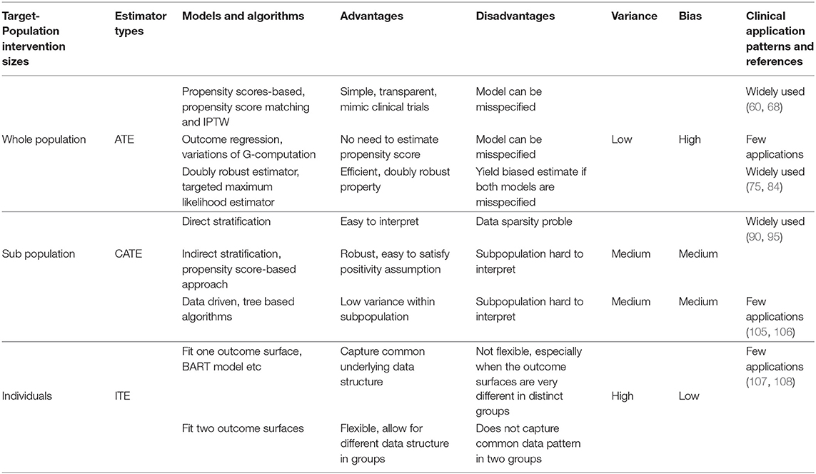
Table 1. Summary of causal inference approaches in healthcare.

We believe that lower historical adoption of more modern observational causal inference approaches is sensible, but that it also represents a gap in the field, especially given the potential promise of more personalized medicine using ITE-type estimators. This gap could potentially be closed in the near future by collaborative pairing of biostatisticians and machine learning scientists with clinicians.

Flowchart for Algorithm Selection

In this section we provide a guide in Figure 1 to help the healthcare community choose which algorithm to use in estimating treatment effects based on the target-population intervention sizes, domain knowledge about the treatment, and track record of healthcare applications of the algorithm. While every problem is unique, and individual judgement must always be exercised, this flowchart can act as a starting point to determine which algorithmic approach may be most appropriate.

FIGURE 1

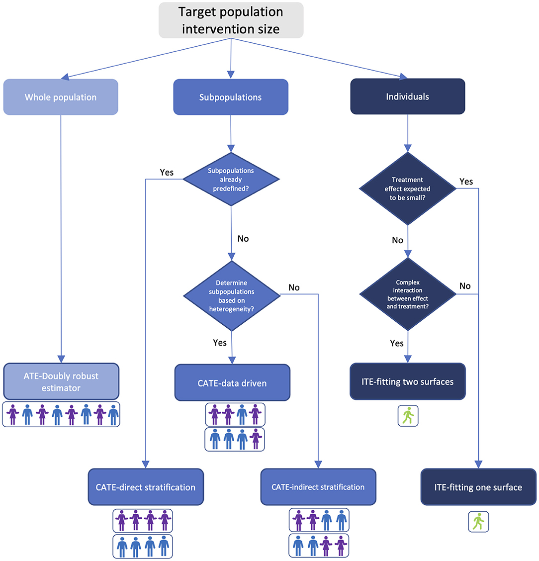
Figure 1. Treatment effect estimator selection guide based on target-population intervention size and prior knowledge. Colors in the figure indicate bias-variance tradeoff. Light blue: high bias and low variance; blue: medium bias and variance; dark blue: low bias and high variance. Person icons under each estimator illustrate the composition of the targeted population.

Discussion

In this paper we reviewed the literature on causal inference with a focus on clinical settings, in light of recent advances in machine learning and large scale EHR adoption. With this review, the algorithm selection guide, and the summary table, we hope to help researchers and healthcare stakeholders gain better understanding of causal inference and make informed decisions on what estimator to use in their daily practices when many choices are on the table.

We have observed that sophisticated causal models based on state-of-the-art machine learning have not been widely applied in clinical studies for a myriad of reasons such as lack of similarity to RCTs and explainability (Section Clinical Applications of Causal Inference), computational intractability of these models, and the healthcare participants being highly conservative when adopting new models. To address the same issue and improve model transparency, a MI-CLAIM check list in Norgeot et al. (109) was proposed regarding the study design of projects, preparation and usage of data, model selection, performance evaluation, model validation, and data pipelines. Our review stresses the importance to follow these guidelines to promote trust on sophisticated models among clinical practitioners.

There are some limitations of the review. First, it may not be exhaustive and include every approach. Causal inference is a very broad topic. While we can limit our review to a specific topic to be exhaustive, it is also important to survey the entire field of causal inference, thus sacrificing the completeness to some degree. Second, causal inference approaches are grouped into ATE, CATE, and ITE categories in this review. These categories might not be mutually exclusive. Such classification, however, does provide an intuitive way for medical professionals to understand causal inference from patient perspectives. Third, there are certain limitations of using citations to rank the applications. For instance, an algorithm applied in clinics might not have been published. Additionally, for a recent work, the citation number might be low, and might not accurately reflect the application potential of the work. Fourth, Table 1 and Figure 1 do not cover all the details of choosing an algorithm, nor do they lead a user to a specific algorithm. They were designed to provide all healthcare participants with an initial but intuitive guide on what family of algorithms to choose for their studies. Finally, our search to find published applications of causal models may not be exhaustive. The search results show that the application disparity of different models is so huge that a different (and potentially more comprehensive) search strategy will unlikely change our conclusions and insights in any significant way.

There is a view in the literature that causal inference is just plain statistical inference, especially after the causal assumptions and parameters are identified (110). The role of causal inference with respect to statistical analysis remains a debate. This debate is out of scope for this paper. We refer to the reviewed models as causal inference models without endorsing any particular view on this matter, but simply use this name to refer to the statistical inference models that reveal causal relationships.

In summary, we reviewed a diverse and complex field of causal inference applied in health care. We distilled the many approaches into three algorithmic families based on the target-population intervention size. We explained the approach type, population size, and bias-variance tradeoff. We then investigated the clinical application of each of the approaches. We finally consolidate all the information into an algorithm selection guide for both researchers and other healthcare stakeholders to decide on which algorithm is applicable to their studies.

Author Contributions

JS conducted the research and developed the figures. BN conceived of the research topic and wrote the manuscript. Both authors contributed to the article and approved the submitted version.

Funding

The authors JS and BN are employed by Anthem, Inc. The funder had no other involvement in the study design, collection, analysis, interpretation of data, the writing of this article, or the decision to submit it for publication.

Conflict of Interest

JS and BN are employed by Anthem, Inc.

Publisher's Note

All claims expressed in this article are solely those of the authors and do not necessarily represent those of their affiliated organizations, or those of the publisher, the editors and the reviewers. Any product that may be evaluated in this article, or claim that may be made by its manufacturer, is not guaranteed or endorsed by the publisher.

Acknowledgments

The authors gratefully acknowledge Chris Jensen for his assistance submitting this work, Paula Alves for her helpful discussions, Abhishaike Mahajan, Daniel Brown, and Dong Wang for proofreading the manuscript.

Supplementary Material

The Supplementary Material for this article can be found online at: https://www.frontiersin.org/articles/10.3389/fmed.2022.864882/full#supplementary-material

References

1. Health IT Dashboard. Available online at: https://dashboard.healthit.gov/quickstats/pages/physician-ehr-adoption-trends.php

Google Scholar

2. Adler-Milstein J, Holmgren AJ, Kralovec P, Worzala C, Searcy T, Patel V. Electronic health record adoption in US hospitals: the emergence of a digital “advanced use” divide. J Am Med Inform Assoc. (2017) 24:1142–8. doi: 10.1093/jamia/ocx080

PubMed Abstract | CrossRef Full Text | Google Scholar

3. Goodman KE, Pineles L, Magder LS, Anderson DJ, Ashley ED, Polk RE, et al. Electronically available patient claims data improve models for comparing antibiotic use across hospitals: results from 576 US facilities. Clin Infect Dis. (2021) 73:e4484–92. doi: 10.1093/cid/ciaa1127

PubMed Abstract | CrossRef Full Text | Google Scholar

4. Das S, Dey A, Pal A, Roy N. Applications of artificial intelligence in machine learning: review and prospect. Int J Comput Applic. (2015) 115:31–41. doi: 10.5120/20182-2402

CrossRef Full Text | Google Scholar

5. Yao L, Chu Z, Li S, Li Y, Gao J, Zhang A. A survey on causal inference. ACM Trans Knowl Discov Data. (2021) 15:1–46. doi: 10.1145/3444944

CrossRef Full Text | Google Scholar

6. Guo R, Cheng L, Li J, Hahn PR, Liu H. A survey of learning causality with data: problems and methods. ACM Comput Surv. (2020) 53:1–37. doi: 10.1145/3397269

CrossRef Full Text | Google Scholar

7. Ding P, Li F. Causal inference: a missing data perspective. Stat Sci. (2018) 33:214–37. doi: 10.1214/18-STS645

PubMed Abstract | CrossRef Full Text | Google Scholar

8. Landsittel D, Srivastava A, Kropf K. A narrative review of methods for causal inference and associated educational resources. Qual Manag Health Care. (2020) 29:260–9. doi: 10.1097/QMH.0000000000000276

PubMed Abstract | CrossRef Full Text | Google Scholar

9. Stuart EA. Matching methods for causal inference: A review and a look forward. Stat Sci. (2010) 25:1–21. doi: 10.1214/09-STS313

PubMed Abstract | CrossRef Full Text | Google Scholar

10. Shah RB, Laupacis A, Hux EJ, Austin CP. Propensity score methods gave similar results to traditional regression modeling in observational studies: a systematic review. J Clin Epidemiol. (2005) 58:550–9. doi: 10.1016/j.jclinepi.2004.10.016

PubMed Abstract | CrossRef Full Text | Google Scholar

11. Austin PC. Propensity-score matching in the cardiovascular surgery literature from 2004 to 2006: a systematic review and suggestions for improvement. Surg Acqu Cardiovasc Dis. (2007) 134:1128–35. doi: 10.1016/j.jtcvs.2007.07.021

PubMed Abstract | CrossRef Full Text | Google Scholar

12. Rosenbaum PR, Rubin DB. The central role of the propensity score in observational studies for causal effects. Biometrilca. (1983) 70:41–55. doi: 10.1093/biomet/70.1.41

CrossRef Full Text | Google Scholar

13. Robins JM, Rotnitzky A, Zhao LP. Marginal structural models and causal inference in epidemiology. Epidemiology. (2000) 11:550–60. doi: 10.1097/00001648-200009000-00011

PubMed Abstract | CrossRef Full Text | Google Scholar

14. Pearl J. Causal diagrams for empirical research. Biometrika. (1995) 82:669–88. doi: 10.1093/biomet/82.4.669

CrossRef Full Text | Google Scholar

15. Pearl J. Probabilistic Reasoning in Intelligent Systems: Networks of Plausible Inference. Morgan Kaufmann (1988). doi: 10.1016/B978-0-08-051489-5.50008-4

CrossRef Full Text | Google Scholar

16. Lauritzen SL. Graphical Models. Oxford: Clarendon Press (1996).

Google Scholar

17. Robins J. A new approach to causal inference in mortality studies with a sustained exposure period–applications to control of the healthy workers survivor effect. Math Model. (1986) 7:1393–512. doi: 10.1016/0270-0255(86)90088-6

CrossRef Full Text | Google Scholar

18. Greenland S, Pearl J, Robins JM. Confounding and collapsibility in causal inference. Stat Sci. (1999) 14:29–46. doi: 10.1214/ss/1009211805

CrossRef Full Text | Google Scholar

19. Angrist JD, Imbens GW, Rubin DB. Identification of causal effects using instrumental variables. J Am Stat Assoc. (1996) 91:444–55. doi: 10.1080/01621459.1996.10476902

PubMed Abstract | CrossRef Full Text | Google Scholar

20. Pearl J. Comment: graphical models, causality and intervention. Stat Sci. (1993) 8:266–9. doi: 10.1214/ss/1177010894

CrossRef Full Text | Google Scholar

21. Barter RL. Visualization, Prediction, and Causal Inference: Applications in Healthcare. UC Berkeley Electronic Theses and Dissertations, University of California, Berkeley, CA, United States (2019).

Google Scholar

22. Thomas S, Richardson JMR. Single world intervention graphs: a primer. In: Second UAI Workshop on Causal Structure Learning. Bellevue, WA (2013).

Google Scholar

23. Rosenbaum PR, Rubin DB. Constructing a control group using multivariate matched sampling methods that incorporate the propensity score. Am Stat. (1985) 39:33–8. doi: 10.1080/00031305.1985.10479383

CrossRef Full Text | Google Scholar

24. Rosenbaum PR. Observational Studies. New York, NY: Springer-Verlag (2002). doi: 10.1007/978-1-4757-3692-2

CrossRef Full Text | Google Scholar

25. Gu XS, Rosenbaum PR. Comparison of multivariate matching methods: structures, distances, and algorithms. J Comput Graph Stat. (1993) 2:405–20. doi: 10.1080/10618600.1993.10474623

CrossRef Full Text | Google Scholar

26. Austin PC. A critical appraisal of propensity-score matching in the medical literature between 1996 and 2003. Stat Med. (2008) 27:2037–49. doi: 10.1002/sim.3150

PubMed Abstract | CrossRef Full Text | Google Scholar

27. Cochran WG, Rubin DB. Controlling bias in observational studies: a review. Indian J Stat Ser A. (1973) 35:417–46.

Google Scholar

28. Hirano K, Imbens GW, Ridder G. Efficient estimation of average treatment effects using the estimated propensity score. Econometrica. (2003) 71:1161–89. doi: 10.1111/1468-0262.00442

CrossRef Full Text | Google Scholar

29. Rosenbaum PR, Rubin DB. Reducing bias in observational studies using subclassification on the propensity score. J Am Stat Assoc. (1984) 79:516–24. doi: 10.1080/01621459.1984.10478078

CrossRef Full Text | Google Scholar

30. Rubin DB. Using multivariate matched sampling and regression adjustment to control bias in observational studies. J Am Stat Assoc. (1979) 74:318–28. doi: 10.1080/01621459.1979.10482513

CrossRef Full Text | Google Scholar

31. Robins JM, Rotnitzky A, Zhao LP. Estimation of regression coefficients when some regressors are not always observed. J Am Stat Assoc. (1994) 89:846–66. doi: 10.1080/01621459.1994.10476818

CrossRef Full Text | Google Scholar

32. Funk MJ, Westreich D, Wiesen C, Stürmer T, Brookhart MA, Davidian M. Doubly robust estimation of causal effects. Am J Epidemiol. (2011) 173:761–7. doi: 10.1093/aje/kwq439

PubMed Abstract | CrossRef Full Text | Google Scholar

33. Laan MJ, Rubin D. Targeted maximum likelihood learning. Int J Biostat. (2006) 2:11. doi: 10.2202/1557-4679.1043

CrossRef Full Text | Google Scholar

34. Schuler MS, Rose S. Targeted maximum likelihood estimation for causal inference in observational studies. Am J Epidemiol. (2016) 185:65–73. doi: 10.1093/aje/kww165

PubMed Abstract | CrossRef Full Text | Google Scholar

35. Morgan SL, Winship C. Counterfactuals and Causal Inference. Cambridge University Press (2014). doi: 10.1017/CBO9781107587991

CrossRef Full Text | Google Scholar

36. Imbens GW, Rubin DB. Causal Inference for Statistics, Social, and Biomedical Sciences. Cambridge University Press (2015). doi: 10.1017/CBO9781139025751

CrossRef Full Text | Google Scholar

37. Athey S, Imbens G. Recursive partitioning for heterogeneous causal effects. Proc Nat Acad Sci USA. (2016) 113:7353–60. doi: 10.1073/pnas.1510489113

PubMed Abstract | CrossRef Full Text | Google Scholar

38. Breiman L, Friedman J, Stone CJ, Olshen RA. Classification and Regression Trees. Chapman and Hall/CRC (1984).

Google Scholar

39. Breiman L. Random forests. Mach Learn. (2001) 45:5–32. doi: 10.1023/A:1010933404324

CrossRef Full Text | Google Scholar

40. Wang P, Sun W, Yin D, Yang J, Chang Y. Robust tree-based causal inference for complex ad effectiveness analysis. In: Proceedings of the Eighth ACM International Conference on Web Search and Data Mining (Shanghai). (2015). p. 67–76. doi: 10.1145/2684822.2685294

CrossRef Full Text | Google Scholar

41. Meid AD, Ruff C, Wirbka L, Stoll F, Seidling HM, Groll A, et al. Using the causal inference framework to support individualized drug treatment decisions based on observational healthcare data. Clin Epidemiol. (2020) 12:1223–34. doi: 10.2147/CLEP.S274466

PubMed Abstract | CrossRef Full Text | Google Scholar

42. Hill JL. Bayesian nonparametric modeling for causal inference. J Comput Graph Stat. (2011) 20:217–40. doi: 10.1198/jcgs.2010.08162

PubMed Abstract | CrossRef Full Text | Google Scholar

43. Chipman HA, George EI, McCulloch RE. Bayesian ensemble learning. In: NIPS'06: Proceedings of the 19th International Conference on Neural Information Processing Systems (Vancouver). (2006). p. 265–72.

Google Scholar

44. Chipman HA, George EI, McCulloch RE. BART: bayesian additive regression trees. Ann Appl Stat. (2010) 4:266–98. doi: 10.1214/09-AOAS285

PubMed Abstract | CrossRef Full Text | Google Scholar

45. Foster JC, Taylor JMG, Ruberg SJ. Subgroup identification from randomized clinical trial data. Stat Med. (2011) 30:2867–80. doi: 10.1002/sim.4322

PubMed Abstract | CrossRef Full Text | Google Scholar

46. Nie X, Wager S. Quasi-Oracle estimation of heterogeneous treatment effects. Biometrika. (2020) 108:299–319. doi: 10.1093/biomet/asaa076

CrossRef Full Text | Google Scholar

47. Wendling T, Jung K, Callahan A, Schuler A, Shah NH, Gallego B. Comparing methods for estimation of heterogeneous treatment effects using observational data from health care databases. Stat Med. (2018) 37:3309–24. doi: 10.1002/sim.7820

PubMed Abstract | CrossRef Full Text | Google Scholar

48. Alaa AM, Schaar M. Limits of estimating heterogeneous treatment effects: guidelines for practical algorithm design. in International Conference on Machine Learning. Stockholm (2018).

Google Scholar

49. Hahn PR, Murray JS, Carvalho CM. Bayesian regression tree models for causal inference: regularization, confounding, and heterogeneous effects. Bayesian Anal. (2020) 15:965–1056. doi: 10.1214/19-BA1195

CrossRef Full Text | Google Scholar

50. Lu M, Sadiq S, Feaster DJ, Ishwarana H. Estimating individual treatment effect in observational data using random forest methods. J Comput Graph Stat. (2018) 27:209–19. doi: 10.1080/10618600.2017.1356325

PubMed Abstract | CrossRef Full Text | Google Scholar

51. Powers S, Qian J, Jung K, Schuler A. Some methods for heterogeneous treatment effect estimation in high dimensions. Stat Med. (2018) 37:1767–87. doi: 10.1002/sim.7623

PubMed Abstract | CrossRef Full Text | Google Scholar

52. Künzel SR, Sekhon JS, Bickel PJ, Yu B. Meta-learners for estimating heterogeneous treatment effects using machine learning. Proc Natl Acad Sci USA. (2019) 116:4156–65. doi: 10.1073/pnas.1804597116

PubMed Abstract | CrossRef Full Text | Google Scholar

53. Alaa AM, Schaar M. Bayesian inference of individualized treatment effects using multi-task Gaussian processes. in 31st International Conference on Neural Information Processing Systems. Long Beach, CA (2017).

Google Scholar

54. Shalit U, Johansson FD, Sontag D. Estimating individual treatment effect: generalization bounds and algorithms. In: Proceedings of the 34th International Conference on Machine Learning. Sydney, NSW (2017).

Google Scholar

55. Hassanpour N, Greiner R. CounterFactual regression with importance sampling weights. In : Twenty-Eighth International Joint Conference on Artificial Intelligence (Macao). (2019). doi: 10.24963/ijcai.2019/815

CrossRef Full Text | Google Scholar

56. Belthangady C, Stedden W, Norgeot B. Minimizing bias in massive multi-arm observational studies with BCAUS: balancing covariates automatically using supervision. BMC Med Res Methodol. (2021) 21:190. doi: 10.1186/s12874-021-01383-x

PubMed Abstract | CrossRef Full Text | Google Scholar

57. Bengio Y, Courville AC, Vincent P. Representation learning: a review and new perspectives. IEEE Trans Pattern Anal Mach Intell. (2013) 35:1798–828. doi: 10.1109/TPAMI.2013.50

PubMed Abstract | CrossRef Full Text | Google Scholar

58. Shi C, Blei DM, Veitch V. Adapting neural networks for the estimation of treatment effects. In: 33rd Conference on Neural Information Processing Systems (NeurIPS 2019). Vancouver, BC (2019).

Google Scholar

59. Moher D, Liberati A, Tetzlaff J, Altman DG. Preferred reporting items for systematic reviews and meta-analyses: the PRISMA statement. PLos Med. (2009) 6:e1000097. doi: 10.1371/journal.pmed.1000097

PubMed Abstract | CrossRef Full Text | Google Scholar

60. Requena CC, Muriel A, Peñuelas Ó. Analysis of causality from observational studies and its application in clinical research in intensive care medicine. Med Intens. (2018) 42:292–300. doi: 10.1016/j.medine.2018.01.010

PubMed Abstract | CrossRef Full Text | Google Scholar

61. Delaney JW, Pinto R, Long J, Lamontagne F, Adhikari NK, Kumar A, et al. The influence of corticosteroid treatment on the outcome of influenza A(H1N1pdm09)-related critical illness. Crit Care. (2016) 20:75. doi: 10.1186/s13054-016-1230-8

PubMed Abstract | CrossRef Full Text | Google Scholar

62. Graham DJ, Reichman ME, Wernecke M, Zhang R, Southworth MR, Levenson M, et al. Cardiovascular, bleeding, and mortality risks in elderly medicare patients treated with dabigatran or warfarin for nonvalvular atrial fibrillation. Circulation. (2015) 131:157–64. doi: 10.1161/CIRCULATIONAHA.114.012061

PubMed Abstract | CrossRef Full Text | Google Scholar

63. Song M, Fung TT, Hu FB, Willett WC, Longo VD, Chan AT, et al. Association of animal and plant protein intake with all-Cause and cause-specific mortality. JAMA Intern Med. (2016) 176:1453–63. doi: 10.1001/jamainternmed.2016.4182

PubMed Abstract | CrossRef Full Text | Google Scholar

64. Kang BJ, Koh Y, Lim CM, Huh JW, Baek S, Han M, et al. Failure of high-flow nasal cannula therapy may delay intubation and increase mortality. Intensive Care Med. (2015) 41:623–32. doi: 10.1007/s00134-015-3693-5

PubMed Abstract | CrossRef Full Text | Google Scholar

65. Jones SE, Maddocks M, Kon SSC, Canavan JL, Nolan CM, Clark AL, et al. Sarcopenia in COPD: prevalence, clinical correlates and response to pulmonary rehabilitation. Thorax. (2015) 70:213–8. doi: 10.1136/thoraxjnl-2014-206440

PubMed Abstract | CrossRef Full Text | Google Scholar

66. Ziff OJ, Samra M, Kirchhof P, Steeds RP, Kotecha D. Safety and efficacy of digoxin: systematic review and meta-analysis of observational and controlled trial data. BMJ. (2015) 351:h4451. doi: 10.1136/bmj.h4451

PubMed Abstract | CrossRef Full Text | Google Scholar

67. Blackstone EH, Suri RM, Rajeswaran J, Babaliaros V, Douglas PS, Fearon WF, et al. Propensity-Matched comparisons of clinical outcomes after transapical or transfemoral transcatheter aortic valve replacement. Circulation. (2015) 131:1989–2000. doi: 10.1161/CIRCULATIONAHA.114.012525

PubMed Abstract | CrossRef Full Text | Google Scholar

68. Chang SH, Chou IJ, Yeh YH, Chiou MJ, Wen MS, Kuo CT, et al. Association between use of non–vitamin k oral anticoagulants with and without concurrent medications and risk of major bleeding in nonvalvular atrial fibrillation. JAMA. (2017) 318:1250–9. doi: 10.1001/jama.2017.13883

PubMed Abstract | CrossRef Full Text | Google Scholar

69. Bangalore S, Guo Y, Zaza Samadashvili, Blecker S, Xu J, Hannan EL. Everolimus-eluting stents or bypass surgery for multivessel coronary disease list of authors. N Engl J Med. (2015) 372:1213–22. doi: 10.1056/NEJMoa1412168

PubMed Abstract | CrossRef Full Text | Google Scholar

70. Kost K, Lindberg L. Pregnancy intentions, maternal behaviors, and infant health: investigating relationships with new measures and propensity score analysis. Demography. (2015) 52:83–111. doi: 10.1007/s13524-014-0359-9

PubMed Abstract | CrossRef Full Text | Google Scholar

71. Grool AM, Aglipay M, Momoli F, Meehan WP. Association between early participation in physical activity following acute concussion and persistent postconcussive symptoms in children and adolescents. JAMA. (2016) 316:2504–14. doi: 10.1001/jama.2016.17396

PubMed Abstract | CrossRef Full Text | Google Scholar

72. Snowden JM, Caughey AB, Cheng YW. Planned out-of-hospital birth and birth outcomes. N Engl J Med. (2015) 373:2642–53. doi: 10.1056/NEJMsa1501738

PubMed Abstract | CrossRef Full Text | Google Scholar

73. Han HS, Shehta A, Ahn S, Yoon YS, Cho JY, Choi Y. Laparoscopic versus open liver resection for hepatocellular carcinoma: case-matched study with propensity score matching. J Hepatol. (2015) 63:643–50. doi: 10.1016/j.jhep.2015.04.005

PubMed Abstract | CrossRef Full Text | Google Scholar

74. Prati F, Romagnoli E, Burzotta F, Limbruno U, Gatto L, Manna AL, et al. Clinical impact of OCT findings during PCI: the CLI-OPCI II study. J Am Coll Cardiol Img. Nov. (2015) 8:1297–305. doi: 10.1016/j.jcmg.2015.08.013

PubMed Abstract | CrossRef Full Text | Google Scholar

75. Prescott HC, Osterholzer JJ, Langa KM, Angus DC, Iwashyna TJ. Late mortality after sepsis: propensity matched cohort study. BMJ. (2016) 353:i2357. doi: 10.1136/bmj.i2375

PubMed Abstract | CrossRef Full Text | Google Scholar

76. Xie Y, Bowe B, Li T, Xian H, Yan Y, Al-Aly Z. Risk of death among users of proton pump inhibitors: a longitudinal observational cohort study of United States veterans. BMJ Open. (2017) 7:e015735. doi: 10.1136/bmjopen-2016-015735

PubMed Abstract | CrossRef Full Text | Google Scholar

77. Cheetham TC, An J, Jacobsen SJ. Association of testosterone replacement with cardiovascular outcomes among men with androgen deficiency. JAMA Intern Med. (2017) 177:491–9. doi: 10.1001/jamainternmed.2016.9546

PubMed Abstract | CrossRef Full Text | Google Scholar

78. Izurieta HS, Chillarige Y, Kelman J, Wei Y, Lu Y, Xu W, et al. Relative effectiveness of cell-cultured and egg-based influenza vaccines among elderly persons in the United States, 2017–2018. J Infect Dis. (2019) 220:1255–64. doi: 10.1093/infdis/jiy716

PubMed Abstract | CrossRef Full Text | Google Scholar

79. Bailly S, Leroy O, Montravers P, Constantin JM, Dupont H, Guillemot D, et al. Antifungal de-escalation was not associated with adverse outcome in critically ill patients treated for invasive candidiasis: post hoc analyses of the AmarCAND2 study data. Intensive Care Med. (2015) 41:1931–40. doi: 10.1007/s00134-015-4053-1

PubMed Abstract | CrossRef Full Text | Google Scholar

80. Feng M, McSparron JI, Kien DT, Stone DJ, Roberts DH, Schwartzstein RM, et al. Transthoracic echocardiography and mortality in sepsis: analysis of the MIMIC-III database. Intensive Care Med. (2018) 44:884–92. doi: 10.1007/s00134-018-5208-7

PubMed Abstract | CrossRef Full Text | Google Scholar

81. Chaffee BW, Cheng J, Featherstone JD. Baseline caries risk assessment as a predictor of caries incidence. J Dent. (2015) 43:518–24. doi: 10.1016/j.jdent.2015.02.013

PubMed Abstract | CrossRef Full Text | Google Scholar

82. Blumberg SJ, Zablotsky B, Avila RM, Colpe LJ, Pringle BA, Kogan MD. Diagnosis lost: differences between children who had and who currently have an autism spectrum disorder diagnosis. Autism. (2015) 20:783–95. doi: 10.1177/1362361315607724

PubMed Abstract | CrossRef Full Text | Google Scholar

83. Barnes H, Rearden J, McHugh MD. Magnet hospital recognition linked to lower central line-associated bloodstream infection rates. Res Nurs Health. (2016) 39:96–104. doi: 10.1002/nur.21709

PubMed Abstract | CrossRef Full Text | Google Scholar

84. Breslau J, Leckman-Westin E, Yu H, Han B, Pritam R, Guarasi D, et al. Impact of a mental health based primary care program on quality of physical health care. Admin Policy Ment Health Ment Health Serv Res. (2018) 45:276–85. doi: 10.1007/s10488-017-0822-1

PubMed Abstract | CrossRef Full Text | Google Scholar

85. Simon TG, Duberg AS, Aleman S, Chung RT, Chan AT, Ludvigsson JF. Association of aspirin with hepatocellular carcinoma and liver-related mortality. N Engl J Med. (2020) 382:1018–28. doi: 10.1056/NEJMoa1912035

PubMed Abstract | CrossRef Full Text | Google Scholar

86. Ajmal A, Gessert CE, Johnson BP, Renier CM, Palcher JA. Effect of angiotensin converting enzyme inhibitors and angiotensin receptor blockers on hemoglobin levels. BMC Res Notes. (2013) 6:443. doi: 10.1186/1756-0500-6-443

PubMed Abstract | CrossRef Full Text | Google Scholar

87. Millett PJ, Espinoza C, Horan MP, Ho CP, Warth RJ, Dornan GJ, et al. Predictors of outcomes after arthroscopic transosseous equivalent rotator cuff repair in 155 cases: a propensity score weighted analysis of knotted and knotless self-reinforcing repair techniques at a minimum of 2 years. Arch Orthop Trauma Surg. (2017) 137:1399–408. doi: 10.1007/s00402-017-2750-7

PubMed Abstract | CrossRef Full Text | Google Scholar

88. Reed GW, Abdallah MS, Shao M, Wolski K, Wisniewski L, Yeomans N, et al. Effect of aspirin coadministration on the safety of celecoxib, naproxen, or ibuprofen. J Am Coll Cardiol. (2018) 71:1741–51. doi: 10.1016/j.jacc.2018.02.036

PubMed Abstract | CrossRef Full Text | Google Scholar

89. Kawasaki R, Konta T, Nishida K. Lipid-lowering medication is associated with decreased risk of diabetic retinopathy and the need for treatment in patients with type 2 diabetes: a real-world observational analysis of a health claims database. Diabetes Obes Metab J Pharmacol Ther. (2018) 20:2351–60. doi: 10.1111/dom.13372

PubMed Abstract | CrossRef Full Text | Google Scholar

90. Soumerai SB, McLaughlin TJ, Spiegelman D, Hertzmark E, Thibault G, Goldman L. Adverse outcomes of underuse of β-blockers in elderly survivors of acute myocardial infarction. JAMA. (1997) 277:115–21. doi: 10.1001/jama.277.2.115

PubMed Abstract | CrossRef Full Text | Google Scholar

91. Hannan EL, Wu C, Walford G, Culliford AT, Gold JP, Smith CR, et al. Drug-Eluting stents vs. coronary-artery bypass grafting in multivessel coronary disease. N Engl J Med. (2008) 358:331–41. doi: 10.1056/NEJMoa071804

PubMed Abstract | CrossRef Full Text | Google Scholar

92. Ip A, Berry DA, Hansen E, Goy AH, Pecora AL, Sinclaire BA, et al. Hydroxychloroquine and tocilizumab therapy in COVID-19 patients—An observational study. PLoS ONE. (2020) 15:e0237693. doi: 10.1371/journal.pone.0237693

PubMed Abstract | CrossRef Full Text | Google Scholar

93. Lindahl B, Baron T, Erlinge D, Hadziosmanovic N, Nordenskjöld A, Gard A, et al. Medical therapy for secondary prevention and long-term outcome in patients with myocardial infarction with nonobstructive coronary artery disease. Circulation. (2017) 135:1481–9. doi: 10.1161/CIRCULATIONAHA.116.026336

PubMed Abstract | CrossRef Full Text | Google Scholar

94. Kuck KH, Brugada J, Fürnkranz A, Chun KRJ, Metzner A, Ouyang F, et al. Impact of female sex on clinical outcomes in the FIRE AND ICE trial of catheter ablation for atrial fibrillation. Circulation Arrhythm Electrophysiol. (2018) 11:e006204. doi: 10.1161/CIRCEP.118.006204

PubMed Abstract | CrossRef Full Text | Google Scholar

95. Kushida CA, Nichols DA, Holmes TH, Quan SF, Walsh JK, Gottlieb DJ, et al. Effects of continuous positive airway pressure on neurocognitive function in obstructive sleep apnea patients: the apnea positive pressure long-term efficacy study (APPLES). Sleep. (2012) 35:1593–602. doi: 10.5665/sleep.2226

PubMed Abstract | CrossRef Full Text | Google Scholar

96. Conway PH, Cnaan A, Zaoutis T, Henry BV, Grundmeier RW, Keren R. Recurrent urinary tract infections in children risk factors and association with prophylactic antimicrobials. JAMA. (2007) 298:179–86. doi: 10.1001/jama.298.2.179

PubMed Abstract | CrossRef Full Text | Google Scholar

97. Hackam GD, Pharm MM, Li P, Redelmeier DA. Statins and sepsis in patients with cardiovascular disease: a population-based cohort analysis. Lancet. (2006) 367:413–8. doi: 10.1016/S0140-6736(06)68041-0

PubMed Abstract | CrossRef Full Text | Google Scholar

98. Vikram HR, Buenconsejo J, Hasbun R, Quagliarello VJ. Impact of valve surgery on 6-month mortality in adults with complicated, left-sided native valve endocarditis a propensity analysis. JAMA. (2003) 290:3207–14. doi: 10.1001/jama.290.24.3207

PubMed Abstract | CrossRef Full Text | Google Scholar

99. Martin D, Glass TA, Bandeen-Roche K, Todd AC, Shi W, Schwartz BS. Association of blood lead and tibia lead with blood pressure and hypertension in a community sample of older adults. Am J Epidemiol. (2006) 163:467–78. doi: 10.1093/aje/kwj060

PubMed Abstract | CrossRef Full Text | Google Scholar

100. Hannan EL, Racz M, Holmes DR, King SB III, Walford G, Ambrose JA, et al. Impact of completeness of percutaneous coronary intervention revascularization on long-term outcomes in the stent era. Circulation. (2006) 113:2406–12. doi: 10.1161/CIRCULATIONAHA.106.612267

PubMed Abstract | CrossRef Full Text | Google Scholar

101. Wong YN, Mitra N, Hudes G, Localio R, Schwartz JS, Wan F, et al. Survival associated with treatment vs observation of localized prostate cancer in elderly men. JAMA. (2006) 296:2683–93 doi: 10.1001/jama.296.22.2683

PubMed Abstract | CrossRef Full Text | Google Scholar

102. Ferguson TB, Coombs LP, Peterson ED. Preoperative β-blocker use and mortality and morbidity following CABG surgery in north america. JAMA. (2002) 287:2221–7. doi: 10.1001/jama.287.17.2221

PubMed Abstract | CrossRef Full Text | Google Scholar

103. Potosky AL, Harlan LC, Kaplan RS, Johnson KA, Lynch CF. Age, sex, and racial differences in the use of standard adjuvant therapy for colorectal cancer. J Clin Oncol. (2002) 20:1192–202. doi: 10.1200/JCO.2002.20.5.1192

PubMed Abstract | CrossRef Full Text | Google Scholar

104. Ahmed A, Rich MW, Sanders PW, Perry GJ, Bakris GL, Zile MR, et al. Chronic kidney disease associated mortality in diastolic versus systolic heart failure: a propensity matched study. Am J Cardiol. (2007) 99:393–8. doi: 10.1016/j.amjcard.2006.08.042

PubMed Abstract | CrossRef Full Text | Google Scholar

105. Graham C, Lewis S, Forbes J, Mead G, Hackett ML, Hankey GJ, et al. The FOCUS, AFFINITY and EFFECTS trials studying the effect(s) of fluoxetine in patients with a recent stroke: statistical and health economic analysis plan for the trials and for the individual patient data meta-analysis. Trials. (2017) 18:627. doi: 10.1186/s13063-017-2385-6

PubMed Abstract | CrossRef Full Text | Google Scholar

106. Lee K, Small DS, Hsu JY, Silber JH, Rosenbaum PR. Discovering effect modification in an observational study of surgical mortality at hospitals with superior nursing. J Am Stat Assoc. (2018) 181:535–46. doi: 10.1111/rssa.12298

CrossRef Full Text | Google Scholar

107. Guo S, Wang YL, Li Y, Jin L, Xiong M, Ji QH, et al. Significant SNPs have limited prediction ability for thyroid cancer. Cancer Med. (2014) 3:731–5. doi: 10.1002/cam4.211

PubMed Abstract | CrossRef Full Text | Google Scholar

108. Esposito MH, Lee H, Hicken MT, Porter LC, Herting JR. The consequences of contact with the criminal justice system for health in the transition to adulthood. Longit Life Course Stud. (2017) 8:57–74. doi: 10.14301/llcs.v8i1.405

PubMed Abstract | CrossRef Full Text | Google Scholar

109. Norgeot B, Quer G, Beaulieu-Jones BK, Torkamani A, Dias R, Gianfrancesco M, et al. Minimum information about clinical artificial intelligence modeling: the MI-CLAIM checklist. Nat Med. (2020) 26:1320–4. doi: 10.1038/s41591-020-1041-y

PubMed Abstract | CrossRef Full Text | Google Scholar

110. Maya L, Petersen MJL. Causal models and learning from data. Epidemiology. (2014) 25:418–26. doi: 10.1097/EDE.0000000000000078

PubMed Abstract | CrossRef Full Text | Google Scholar