Dopant network processing units as tuneable extreme learning machines

Introduction

Spurred by the increasing computational demands of artificial intelligence (AI), the difficulties of conventional computing hardware to keep up with these demands, and inspired by the highly efficient information processing of the brain, there is a growing interest in harnessing chemical and physical phenomena in material systems for complex, efficient computations (Kaspar et al., 2021). This growing field of research goes by different names, such as unconventional, natural or in-matter computing (Zauner, 2005; Miller et al., 2018). Designing a material system as a computing device is a non-trivial task, especially on the nanoscale. Instead, one can train certain designless, disordered material systems to exhibit functionality, a process we refer to as “material learning” (Chen et al., 2020), in analogy to “machine learning” in software systems. In these disordered material systems, a single trainable parameter influences the whole system. This global tuneability can potentially reduce the number of parameters that need to be stored subsequently, reducing the necessary communication between the memory and processing units (Sze et al., 2017).

A recent example of a designless, tuneable nanoscale material system that can be trained for functionality using material learning is a dopant network processing unit (DNPU) (Chen et al., 2020). It consists of a network of donor or acceptor dopant atoms in a semiconductor host material. Transport is dominated by hopping and Coulomb interactions, giving rise to strongly non-linear IV characteristics, including negative differential resistance (NDR) (Tertilt et al., 2022). Charge carriers hop from one dopant atom to another under the influence of input and control voltages applied at surrounding electrodes. The output consists of the current(s) measured at one or more electrodes. For material learning using DNPUs, their electronic properties should be tuneable, non-linear, and exhibit negative differential resistance (NDR). This can be realised by varying one or more control voltages, as shown in Figure 1A. Among other things, DNPUs have been shown to have the capability of solving non-linear classification tasks (Chen et al., 2020). There are several methods to obtain desired functionality in DNPUs by material learning. We have demonstrated DNPU training with artificial evolution (Miller and Downing, 2002), off-chip gradient descent (Ruiz Euler et al., 2020), and more recently, gradient descent in matter (Boon et al., 2021).

FIGURE 1

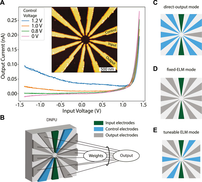
FIGURE 1. Dopant Network Processing Units as tuneable extreme learning machines: (A) IV curves measured between an input and an output electrode of a 12-electrode dopant network processing unit (DNPU), for different control voltages applied to a third control electrode (0 V is applied to the other electrodes), exhibiting negative differential resistance (NDR) when the control voltage increases (orange and blue curves). Inset: atomic force microscope (AFM) image of the DNPU. (B) Schematic of a DNPU used in the “tuneable ELM mode”, with input (green), output (grey) and control (blue) electrodes. The final output of the system is obtained by linearly combining the output currents with tuneable weights. (C) Schematic of the conventional, ‘direct-output mode’. In this case there is a single output (without linear weight factor), while the other electrodes are either used as input or control. (D) Schematic of the ‘fixed-ELM mode’: all electrodes are either inputs or outputs, where the latter are linearly combined to form the output. (E) Schematic of the “tuneable ELM mode”, which is a hybrid of the modes shown in (C) and (D).

In-matter artificial evolution is a material-learning approach in which (digital) computer-controlled evolution is used to manipulate a physical system. It allows the exploitation of complex physical effects, even if these effects are a priori unknown (Miller et al., 2014). Off-chip gradient descent is an approach where an artificial neural network (ANN) is trained to emulate the behaviour of the physical DNPU. This allows the use of standard deep-learning methods to determine the control voltages that are needed to reach a desired functionality (Ruiz Euler et al., 2020). Gradient descent in matter is a method that uses lock-in techniques to extract the gradient in the output with respect to the tuneable parameters by perturbing these parameters in parallel with different frequencies. Using the extracted gradient, it is possible to gradually move towards a desired functionality directly in the material system (Boon et al., 2021).

Another popular framework for utilising the complexity of disordered material systems is reservoir computing (RC). Independently developed RC schemes are echo state networks (ESNs) (Jaeger, 2010), liquid state machines (LSMs) (Maass et al., 2002), and the backpropagation-decorrelation (BPDC) on-line learning rule (Steil, 2004). Generally, the concept of RC was used in combination with recurrent neural networks (RNNs), which exhibit time-dependent (dynamic) behaviour (Lukoševičius and Jaeger, 2009). Here, the network (reservoir) projects input values non-linearly into a high-dimensional space of its reservoir states. To train such a network to perform a certain task, a linear, supervised reservoir readout layer is used to map the reservoir states to a desired output. As only the weights of the readout layer need to be trained, while the random network itself remains fixed during the training process, the training is relatively fast and efficient as compared to other neural network training methods (Tanaka et al., 2019). Its general applicability makes RC a suitable approach to utilise disordered material-based networks to perform desired computations, as has been shown, for example, in network of carbon nanotubes (Dale et al., 2016) and polymers (Usami et al., 2021). Another approach that linearly combines the output states of a network is that of extreme learning machines (ELMs) (Wang et al., 2021). Recent work shows that a physical ELM is equivalent to a physical RC system without time dynamics. An opto-electronic network is used to implement both an RC system and an ELM, based on a switch that turns a feedback loop on or off, changing the network from a time-dependent to a time-independent system (Ortín et al., 2015). Figure 1B) illustrates a 12-electrode DNPU operated in the tuneable ELM mode, where the black lines indicate the weighted connections of the readout layer mapping the DNPU’s output states (currents) to the desired output of the network.

In the present study we move from 8-electrode DNPUs used in our previous work (Chen et al., 2020; Ruiz Euler et al., 2020; Ruiz-Euler et al., 2021) to a 12-electrode DNPU to increase the computational capabilities of DNPUs based on boron-doped silicon. To further increase the computational capabilities of this 12 electrode DNPU, we operate this DNPU in the tuneable ELM mode. This tuneable ELM approach is inspired by the work of Dale et al, (2017), who showed that by combining the concept of RC with in-matter artificial evolution, it is possible to obtain a reservoir capable of reaching higher accuracies for RC benchmark tasks (Dale et al., 2016; Dale et al., 2017). Their work mainly focusses on the use of micron-scale carbon nanotube/polymer mixtures. DNPUs are different from these systems in several ways. On the one hand, they have a smaller footprint and are silicon-based, which may facilitate scaling and integration with conventional electronics. On the other hand, DNPUs do not exhibit time dynamics at the timescales of our measurements, which holds if the measurements are performed below 1 MHz (Tertilt et al., 2022). This makes these systems, in their present form, unsuitable to process data directly in the time domain, but more suitable for the ELM approach. The advantage of physical ELMs over physical RC systems is the compatibility with the off-chip gradient descent training technique (Ruiz Euler et al., 2020). This training technique allows incorporation of the DNPU performing the ELM function in bigger networks of coupled DNPUs and other ANN elements to create a new combined network that can be trained in one training run, after which the task can be implemented in the material platform. This could lead to a universal training technique allowing for the use of different material platforms (e.g., a DNPU as tuneable non-linear ELM combined with memristor technology for linear operations) to be optimised at the same time.

In Figure 1A, we show that a DNPU needs so-called control or tuning electrodes to achieve negative differential resistance (NDR). NDR is necessary to perform complex non-linear classification tasks such as achieved by the XOR Boolean logic gate (Bose et al., 2015; Chen et al., 2020). When moving from the single-output mode to the tuneable ELM mode, the question is to what degree tuneability is necessary to extract the most non-linear computation from a DNPU. This is investigated by studying the computational power of a DNPU in the tuneable ELM operation mode for different numbers of control (N_C) and output (N_O) electrodes, using two input electrodes. To quantify computational power we use the Vapnik-Chervonenkis, VC dimension (Ruiz-Euler et al., 2021), defined as the maximum number of non-collinear points that can be classified into all possible binary groups. Since it is a priori not known how many control and output electrodes are needed to realise the highest computational capability, we study multiple tuneable ELM modes, going from the standard direct-output mode (N_C = 9, N_O = 1, Figure 1C) to the fixed-ELM mode (N_C = 0, N_O = 10, Figure 1D). As an example, a tuneable ELM mode with N_C = 4, N_O = 6 is schematically represented in Figure 1E. First, we search for the optimal operation mode for performing binary classification tasks. For the optimal operation mode, we demonstrate the use of the off-chip gradient descent training technique (Ruiz Euler et al., 2020) to perform the formant-based vowel recognition benchmark task (Hillenbrand, 2009) with up to five emulated DNPUs in parallel. Finally, we will use the vowel recognition benchmark to show that using DNPUs as tuneable ELMs allows one to reduce the number of parameters that need to be tuned and stored as compared to an ANN counterpart. Our results emphasise the power of in-matter computing and underline the importance of combining different material platforms in a way that optimises their computational capabilities.

Results

VC dimension analysis

In Figure 2A the measurement scheme of the VC dimension analysis is presented. To perform this analysis, seven input points are defined in a two-dimensional voltage input space (as represented by the two waveforms in the left part of Figure 2A). These points are chosen within the working range of −1.1 to 1.1 V of the DNPU that we used for our study. In Figure 2B, the points used to create the input voltage waveforms V_in1, V_in2 are plotted against each other. The first four input points are chosen such that for the fixed-ELM mode VC dimension four can be realised. To avoid collinearity, the other points are chosen by placing them collinearly on the line connecting two points and shifting them from this line to lift collinearity. Point 5 is placed in between point 1 and 3 and shifted along the V_in1 input. Point 6 is placed in between points 2 and 4 and shifted along the V_in2 axis. Point 7 is placed in between points 1 and 4 and shifted both along the V_in1 and V_in2 axis. The shifts are chosen in a similar way as by Ruiz-Euler et al, (2021) and such that a good spread of points is obtained. Using these input points, the complexity of the task can be varied by the number of points that need to be correctly labelled by the tuneable DNPU ELM (Figure 2A, middle part), where a perceptron is used to determine when the points are correctly labelled (see Methods). For each n input points there are 2ⁿ possible labels. In Figure 2A, the DNPU and the linear layer are trained to yield as output the binary label [0000110], which is one of the 2⁷ = 128 labels for VC dimension 7.

FIGURE 2

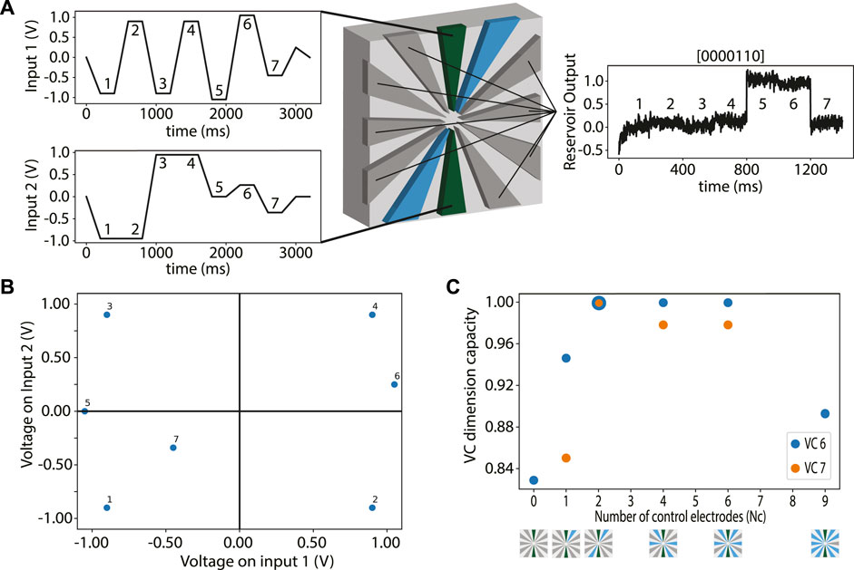
FIGURE 2. VC dimension analysis: (A) Schematic of the VC dimension benchmark for the raw input waveforms on the left using the DNPU (inputs: green, controls: blue, outputs: grey) and the readout layer in a tuneable ELM operation mode, with N_C = 2 control electrodes and N_O = 8 output electrodes (middle). The output waveform of label [0000110] for VC dimension seven is displayed on the right, where only the output at the plateaus of the input is shown. (B) Schematic of the seven voltage input points labelled one to seven to indicate which points are used for the analysis of the VC dimension 1–7. (C) The capacity (fraction of correct labels) for the different operation modes, indicated by the number of control electrodes used. Blue: VC dimension 6 (6 input points). Orange: VC dimension 7 (7 input points, only for the tuneable ELM modes). The DNPU schematics at the x-axis show the electrode configurations.

The training of the DNPU ELM is performed using a combination of a computer-assisted genetic algorithm (GA) (Such et al., 2017), to find the voltages needed to tune the ELM, and pseudoinverse learning (Tapson and van Schaik, 2013), to find the optimal weights in the linear readout layer. For each genome (set of control voltages) in the genetic algorithm, new weights for the readout layer are found using pseudoinverse learning, after which the output of the network is mapped to a class probability using a perceptron (see Methods). For VC dimension 6 (blue points) and 7 (orange points) several different tuneable ELM modes have been studied, see Figure 2C: N_C = 0, 1, 2, 4, six and nine for VC dimension 6. The N_C = 0 and N_C = 9 cases are the direct output and fixed-ELM modes, respectively. All values of N_C in between correspond to the tuneable ELM modes. Because for VC dimension six the tuneable ELM modes have the highest computational capacity, we only analyse these further for VC dimension 7. We observe that the N_C = 2 mode has the highest computational capability, since this operation mode has the highest capacity for VC dimension 7.

We now investigate how diversified the outputs from the terminals are when increasing the number of output terminals of a DNPU. In the field of RC and ELMs, in general, having more output states (output channels) in the network results in the capability of solving more complex tasks. However, this is only valid when the output states are linearly separable from one another (Legenstein and Maass, 2007; Dale et al., 2019). The linear separability of the output states can be quantified by calculating the rank of the output matrix, where the highest possible rank equals the number of output states (Legenstein and Maass, 2007). In our case, for both the full-ELM mode (N_C = 0) and the optimal tuneable ELM mode (N_C = 2, for the case used to generate Figure 3B) the rank of the output matrices is 7, meaning that there are seven linearly separable outputs. Here we expect that the increase in the VC dimension for the N_C = 2 case originates from the added tuneability the control electrodes provide. To investigate this behaviour, we analyse the correlations in the DNPU output states. This is done by calculating the Pearson correlation coefficient between all the output currents of the fixed-ELM mode, as shown in Figure 3A. It is observed that most of the correlations between the outputs are relatively high (dark blue). Outputs 1 and 10 as well as five and six even have a correlation coefficient of 1.00, meaning that they provide the same information. Therefore, using output electrodes one and six instead as control electrodes does not result in a loss of information, while allowing to tune the DNPU towards a more complex output response. Based on this observation, the choice which electrodes to use as control for the N_C = 1, two modes is straightforward. For the other two tuneable ELM modes (N_C = 4, 6) the control electrodes were chosen such that at least one output or input electrode is in between the control electrodes, resulting in the DNPU schematics shown in Figure 2C. To further illustrate this choice. We show the correlation matrices for N_C = 2 for the label [0000101] in Figure 3B. On average, the correlation coefficients are closer to 0, showing the increased variability between the outputs. This also shows the limitation of using the rank of the output matrix to analyse the linear separability of the output states. Although we know how many output states are linearly separable, we do not gain information about the degree of separability. Here the correlation coefficients we calculated help to gain a more in-depth understanding of the behaviour of the output states. Since the number of output states limits the performance of the ELM, it is likely that better results can be achieved if the DNPU has more electrodes to both allow for a higher degree of tuneability and an increase of the number of output states. In this case it might be possible to achieve a single set of control voltages capable of solving VC dimension 7, where, for the N_C = 2 case, we had to retrain the DNPU multiple times to get the necessary information in the output states.

FIGURE 3

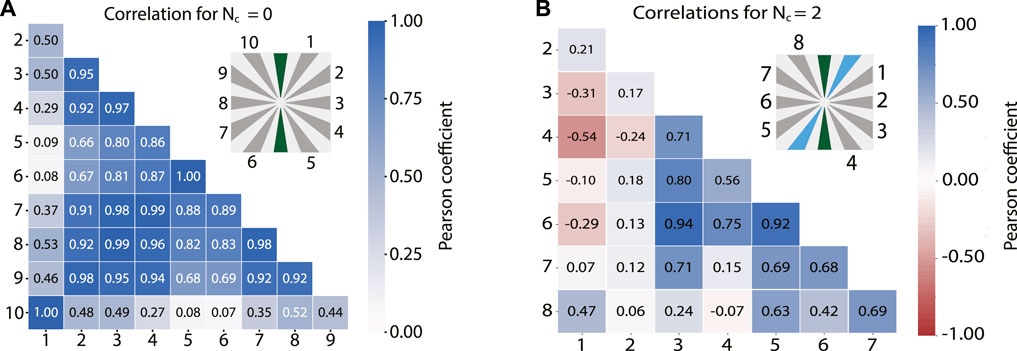
FIGURE 3. Correlation matrices. (A) Correlation matrix of the output currents of the DNPU for the fixed ELM mode (N_C = 0) for VC dimension 7. The darker the blue, the higher the correlation in the output currents. (B) Correlation plot for label 5 ([0000101]) of the outputs of the DNPU in the N_C = 2 tuneable ELM mode.

Vowel recognition using tuneable DNPU ELMs

To demonstrate the capability of the DNPU to perform more complex tasks, we focus on the Hillenbrand formant-based vowel recognition benchmark task (Hillenbrand, 1995). For this task, we emulate the behaviour of multiple DNPUs in parallel. The behaviour of all DNPUs is derived from a single physical DNPU, so we “cloned” a single DNPU. Formant-based vowel recognition is a classification benchmark with a limited number of features and classes, making it a task that can be solved with a limited number of DNPU ELMs. Hillenbrand, 1995) extracted the formants from recordings of a spoken vowel at different times, which are the broad spectral acoustic maxima caused by acoustic resonances in the human vocal tract. This allows the transformation of a task that is commonly performed using dynamic systems to a static benchmark task, making it compatible with DNPUs. Adult male/female as well as boy/girl speakers each pronounced 12 different vowels. From the recordings, a dataset was constructed by first extracting the fundamental frequency or pitch f₀, which is the lowest frequency present in a spoken vowel. This frequency is directly linked to the size of the speaker’s vocal cords. Therefore, men tend to have a low f₀ and women a high f₀. This is a useful measure to take into account when classifying over different ages and genders, as is done in this benchmark (Pernet and Belin, 2012).

After determining f₀, Hillenbrand et al. extracted four formants before the vowel is spoken (known as the “steady state”) and three formants at 20%, 50% and 80% of the spoken vowel duration. In Figure 4A we show a spectrogram of the vowel “oa” pronounced by an adult male, where the vertical features indicate the different formant frequencies and the horizontal lines the times at which they have been extracted. This results in a total of 14 features to be used as the inputs for the task. See Methods for an elaboration on the Hillenbrand data set and how the formants are mapped to the input for the DNPU.

FIGURE 4

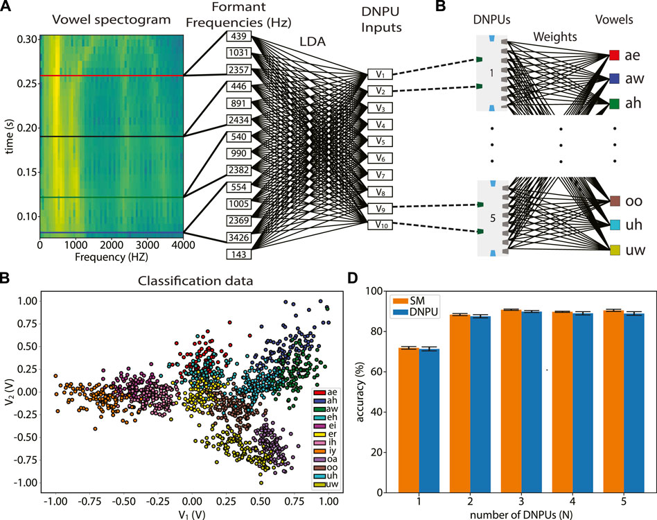
FIGURE 4. Spoken vowel recognition task: (A) Left: spectrogram of an adult male pronouncing “oa”. The horizontal lines indicate the times at which the formants are extracted. Right: mapping of formant frequencies to voltages V₁-V₁₀ using linear discriminant analysis (LDA). (B) V₂ versus V₁ for all 12 vowels, showing overlap, especially for V₂. (C) Vowel classification by N DNPUs in parallel, with a linear readout layer: V₁ and V₂ are inputs to DNPU₁, V₃ and V₄ are inputs to DNPU_2, etc. (D) Classification accuracies for N clones of the physical DNPU and of the surrogate model (SM) of the DNPU.

To use a single DNPU in the N_C = 2 tuneable ELM mode, we need flexibility in the number of inputs. To reduce this number, while still using the information from all 14 features, we use a linear discriminant analysis (LDA), where the input data are linearly mapped to a feature space in which classes have the highest separation (between-class covariance) and lowest within-class covariance, see Supplementary Note S1. After this linear mapping, the input data are normalised to the DNPU input range (−1.0 to 1.0 V). This results in 10 new inputs ordered from the best (V₁) to the worst (V₁₀) classifying input, see Figure 4A. In Figure 4B, V₂ is plotted against V₁. It is seen that the vowels have less overlap when projected to V₁ than to V₂, as is expected when using LDA. To demonstrate the computational capabilities of the DNPUs without needing to fabricate several of them, we use the single DNPU analysed above and measure its output currents when either V₁ and V₂, V₃ and V₄, etc., are applied as input voltages. This corresponds to putting N = one to five identical “cloned” DNPUs in parallel. Effectively, this corresponds to using five different DNPUs, because the control voltages of the cloned DNPUs will be different, leading to completely different input-output characteristics (in the next paragraph we explain how the control voltages are determined). For the cases with N < 5, the last 2×(5−N) inputs are discarded. Finally, we use a single linear readout layer with as inputs the measured currents, as stored in a digital computer, of the N clones of the DNPU; see Figure 4C. We call this method of performing the vowel recognition task, where we use a physical device in combination with operations performed in a computer, a “hybrid” method. We note that the measured currents contain noise and other uncertainties that are also present in a fully physical implementation.

In addition to the network with the cloned physical DNPU, a network is created with N clones of an ANN surrogate model (SM) of the DNPU that accurately emulates its behaviour (Ruiz Euler et al., 2020). To train this network for the vowel recognition task, we use the off-chip gradient descent-based training technique we introduced in Ref. (Ruiz Euler et al., 2020). We extend that work by including the linear readout layer in a complete ANN model of the full network (the SM and the linear readout layer; see Figure 4C). This allows us to use standard deep-learning methods to train the complete network for the vowel recognition task. The found N pairs of control voltages are applied to the physical DNPU, after which the vowel recognition is performed with the hybrid method.

Figure 4D shows the accuracies in the vowel recognition after the training, both for the networks with N clones using the DNPU SM (orange, SM method) and the physical DNPU (blue, hybrid method). For each N, we performed six training runs (see “Methods”), of which we chose the five attempts with the highest recognition accuracy to remove potential outliers. The average values and standard deviations of these five attempts were used to obtain the reported accuracies and error bars. We observe an increase in average accuracy from 71.4% to 89.9% for the hybrid method between N = 1 and N = 3. The saturation in accuracy when N is further increased is attributed to the limited added information in V₇-V₁₀. This can be directly linked to the LDA method, where the first LDA components have the largest linear separability (least overlap) and the last LDA components the smallest. We elaborate on this in Supplementary Note S1 and provide an illustration in Supplementary Figure S1.

We also observe in Figure 4D that transferring the control voltages found in the SM method to the hybrid method results in very limited performance loss (from 90.6% to 89.9% for N = 3). This shows the robustness of the SM method. The small performance loss is attributed to remaining model uncertainties in the SM and the inability of the SM to account for noise. In Supplementary Figure S2 we show that when replacing the LDA by a trainable linear layer with 14 inputs and 2N outputs in a further extended ANN model, we can increase the highest accuracy obtained in the vowel recognition task from 90.6% to 92.6% for the SM method. A similar improvement is expected for the hybrid method.

Parameter reduction using DNPU ELMs

In this subsection, we show that the number of tuneable parameters needed in the vowel recognition task using DNPUs is, for a comparable accuracy, much less than using ANNs. We consider the network structure discussed in the previous subsection; see Figure 4. We use ANNs with two inputs and eight outputs, equal to those of the DNPU in the optimal tuneable ELM mode (N_C = 2, N_O = 8; see Figure 2). To reach a comparable recognition accuracy as with (cloned) DNPUs, the ANNs can be much smaller than the ANN used in the surrogate model (SM) of the DNPU. We use as ANN structure a fully-connected non-linear network between the inputs and the outputs with a ReLU activation function (see “Methods”). Using N = one to five of these small ANNs, illustrated in Figure 5A with the red boxes, we make a network with the same structure as that in Figure 4, but with the ANNs replacing the (cloned) DNPUs. We train this network and use it to perform the vowel recognition task from the previous subsection. Figure 5B compares the achieved average accuracy and error (green) to the ones achieved using the DNPU (blue). The accuracy and error were obtained in the same way as in the previous subsection (extracted from five of the six training runs). We see that, especially for high N, the average accuracies of the hybrid measurements using cloned DNPUs are quite close to those of the ANNs (89.9%, as compared to 91.4% for N = 3).

FIGURE 5

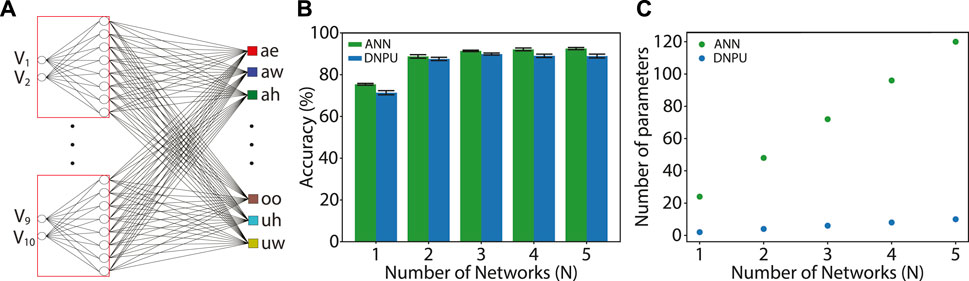
FIGURE 5. Parameter reduction using DNPUs: (A) Same network as in Figure 4C, but with the DNPUs replaced by single-layer fully-connected ANNs (red boxes). (B) Vowel recognition accuracy for the network with ANNs (green) as compared with the network with DNPUs (blue, same data as in Figure 4D). (C) Number of tuneable parameters for the network with ANNs (green) compared with the network with DNPUs (blue).

Since one of the important limitations of deep learning is the storage and retrieval of the values of the parameters used in an ANN (Xu et al., 2018), it is important to reduce the number of parameters. For an ANN, the number of parameters is equal to the number of weights and biases. In Figure 5C, the number of parameters (weights + biases for the ANNs and control voltages for the DNPU) of the ANN replacing the DNPU in the network is plotted against N (green: 24N). For the DNPU case, the number of parameters is equal to the number of control voltages (blue: 2N). The reason why the number of parameters for the DNPU case is smaller than that for the ANN case is that the control voltages of the DNPU have a global effect on the outputs (Chen et al., 2020). While for the DNPU one parameter influences all outputs, for the ANN one parameter influences only one output. In the context of ELM/RC frameworks, this is not a surprising result. However, it does emphasize an important advantage of implementing ELMs and RCs in analog hardware. We note that in the consideration of the number of parameters, we did not take account the weights in the linear readout layer. The reason is that we want to focus on the capabilities of the DNPU itself, which can be exploited in various other tasks than only vowel recognition. We conclude that their global tuning capability in combination with their non-linear input-output relation can make DNPUs a powerful tool for in-matter computation.

Discussion

We have studied the computational power of a dopant network processing unit (DNPU), consisting of a region with boron dopants at the surface of a silicon substrate, contacted with 12 electrodes that can be used as data inputs, controls and outputs. We used the complex non-linear dependence between input voltages and output currents of the DNPU, tuned by voltages applied to the control electrodes, in combination with a linear readout layer. Three modes of operation were considered: (1) the “fixed-ELM mode”, (2) the “direct-output mode” and (3) the “tuneable ELM mode”. In the fixed-ELM mode (1), where the DNPU cannot be tuned, all electrodes are used as inputs or outputs. In the direct-output mode (2), the electrodes are used as inputs, tuneable controls and one or more outputs, without using a readout layer. The tuneable ELM mode (3) is a combination of 1 and 2, where the DNPU can be partially tuned by control voltages. We found that the tuneable ELM mode provides the highest computational power, as quantified by the Vapnik-Chervonenkis (VC) dimension. For the case of two data inputs, we found optimal computation power with two controls and eight outputs. The fact that the fixed-ELM mode (10 outputs) has suboptimal computing power was rationalised by considering the output correlation matrix, which shows strong correlations between the two outputs adjacent to the each of the two inputs. In that case the computation power can be increased by using one of these outputs to as a control electrode, leading to a total of two controls. We conclude from this analysis that consideration of the output correlation matrix is important for optimizing the operation mode of a complex tuneable ELM.

We solved the vowel recognition benchmark task by a hybrid network of emulated DNPUs in the optimal tuneable ELM mode in combination with a common linear readout layer, where the dimension of the input data are reduced while maximising the class separation, using linear discriminant analysis (LDA). As training method, an off-chip gradient descent method was applied using a surrogate model (SM) of the physical DNPU, yielding pairs of control voltages that we applied to the physical DNPU for validation. The noise present in the physical DNPU and deviations from the SM lead to only a small decrease in the accuracy of the vowel recognition task in this hybrid method, as compared to using the SM. Since the different pairs of control voltages in the hybrid method effectively correspond to using different DNPUs, the approach is equivalent to a network using different physical DNPUs. It should therefore be possible to extend this approach to large and fully physical networks with a large number of DNPUs, where also the LDA and the linear readout layer are realised by physical systems such as memristors (Yao et al., 2020) and optical networks (Feldmann et al., 2021). Since training of the latter systems is also done by physically implementing the parameters found by artificial neural networks (ANNs) (Yao et al., 2020; Feldmann et al., 2021), it should be possible to incorporate the training of these physical networks in the off-chip training technique in a similar way as demonstrated in the present work. This could potentially lead to physical networks trained for classification tasks that outperform ANNs regarding inference. We showed that the global, non-linear tuneability of a DNPU requires fewer parameters than a minimal ANN that has similar input-output behaviour. Since these parameters should be stored in memory and retrieved for each recognition task, the use of DNPUs instead of ANNs will be less memory intensive.

The vowel recognition task demonstrated in this work was performed with an accuracy of 89.9% on the test dataset by emulating the behaviour of multiple DNPUs from one physical DNPU. An increase to 92.6% accuracy was shown to be possible by training the DNPU and all linear layers instead of employing LDA. These accuracies are similar to those reported in other work: 89% using spin-torque nano-oscillator (Romera et al., 2018) and 93% accuracy using an optical system (Wright et al., 2022). It should be noted however, that in both these other approaches a subset of the data was used that only included female speakers and seven vowels, making the task easier to solve. Since we include both female and male voices of adults and children on all 12 vowels, the classification task is intrinsically more difficult. As we reach similar accuracies on this harder task, we deem it worthwhile exploring our approach further, preferably at room temperature.

The present work shows the power of using designless disordered systems, such as DNPUs, for computation and provides insight into optimally harnessing their computation power. Building on this, we have indicated how such systems can be combined with other physical systems, exploiting each system’s optimal operation type (such as linear vs. non-linear), to create combined networks for analog computing. On the side of the DNPUs, several optimisation steps still need to be taken, such as consistent room temperature operation, increasing the number of electrodes and going beyond two inputs. Besides this, interconnecting technologies is always a non-trivial step that should also be made in this case. At the same time, we did show the importance of non-linear computation and indicated how DNPUs as tuneable ELMs could be optimised to fulfil this role in future analog hardware systems.

Materials and methods

Dopant network processing units

The DNPU used in this work is fabricated in a similar fashion as the one in Chen et al. (2020). The main difference is the number of electrodes: 12 instead of 8. These electrodes are made by e-beam evaporation of 1 nm Ti and 25 nm Pd, placed on top of a boron doped silicon substrate in a circle with a diameter of 300 nm. The boron concentration under the contacts is approximately 2×10¹⁹ cm^-3, which creates an ohmic contact between the electrodes and the substrate. Using the electrodes as a mask, the silicon is etched such that the boron concentration at the receded silicon surface is reduced to approximately 5×10¹⁷ cm^-3, resulting in variable-range hopping at 77K (Chen et al., 2020).

Measurements

All DNPU measurements are performed using a customised dipstick to insert the device into liquid nitrogen (77K). To measure its behaviour, the DNPU is wire bonded to a printed circuit board (PCB) that has 12 IV converters connected, allowing us to use up to 12 output channels. These IV convertors have either 10 MΩ or 100 MΩ feedback resistances, allowing us to measure a current range of −400 nA to 400 nA or −40 nA to 40 nA, respectively. Output electrodes that are close to the input/control electrodes have relatively large output currents and are connected to the 10MΩ IV converters. This allows measuring the full output current range. The electrodes further away from the input/control electrodes are connected to the 100 MΩ IV converters, such that the relatively small output currents can be determined more accurately. We calculate the measured voltages back to current values in nA. During the measurements, the voltages are applied and measured using a national instruments compactDAQ (NI cDAQ-9132) with two modules, one for digital-to-analogue conversion (NI-9264) and one for analogue-to-digital conversion (NI-9202). This measurement system is automated using Python (https://github.com/BraiNEdarwin).

Vapnik chervonenkis dimension training

To train the network (DNPU + linear readout layer) to yield all the binary labels of the corresponding VC dimension n we combine a genetic algorithm (Such et al., 2017) (GA) with pseudoinverse learning (Tapson and van Schaik, 2013). This is done by randomly initialising a set of 25 genomes of control voltages in the range −1.1 to 1.1 V as optimisable parameters. For each genome the current waveforms of all the N_O outputs of the DNPU are measured for the input waveforms given in Figure 2A. This yields elements of an array X of size n×N_O that are linearly combined to obtain the target output waveforms. The N_O weights W of the linear readout layer are calculated using the pseudo-inverse learning method, which solves (Tapson and van Schaik, 2013)

$W=Y_t{X}^{+}(1)$

where Y_t is the target output waveform (consisting of a sequence of 0’s and 1’s) and X⁺ is the pseudoinverse of X. The 25 obtained network output waveforms $Y=W\bullet X$ are evaluated and ranked based on their fitness (F). In this work we define the fitness as the correlation between the actual and the target output waveforms (Y and Y_t), multiplied by a sigmoid function of the separation (sep) between the lowest high (binary 1) and the highest low (binary 0) state, see Eq. 28:

$F=\mathrm{c}\mathrm{o}\mathrm{r}\mathrm{r}\left(Y,Y_t\right)\ast \frac{1}{1+e^{-2\ast \left(\mathrm{s}\mathrm{e}\mathrm{p}-2\right)}}(2)$

Based on the fitness ranking of the present genomes, the next-generation of genomes is spawned by: (1) keeping the five best genomes from the previous generation; (2) slightly altering the five best genomes by introducing small fluctuations to the genes (voltages); (3) generating five genomes by cross-breeding (blend alpha-beta crossover (BLX alpha-beta)) between the five best performing genomes with a certain probability; (4) five genomes are obtained via crossbreeding between the top five and five random genomes; (5) the last five genomes are randomly generated. For details, we refer to https://github.com/BraiNEdarwin. The GA is performed for 25 generations.

After the GA optimization, the combination of control voltages corresponding to the genome with the highest fitness is applied to the DNPU. To determine whether the correct labels are obtained by the DNPU and the linear readout layer we use a perceptron. We train the perceptron with the output waveforms and the correct labels. The perceptron is trained for 200 epochs using adaptive moment estimation (Adam) gradient descent for 200 epochs using a binary cross-entropy loss function (Paszke et al., 2019), with a learning rate of 7 × 10⁻³, beta coefficients for running averages of (0.9, 0.999), a numerical stability constant ε = 10^–3, and a weight decay of 0. After training the perceptron, the accuracy is determined by calculating the correctly obtained labels divided by the total number of labels, where a label is identified as found when 100% accuracy is achieved. For each label, we make two attempt runs of the whole algorithm. A label is correctly classified/found when an accuracy of 100% is reached in one of the two attempts.

Hillenbrand dataset

The Hillenbrand dataset consists of 12 vowels spoken by male, female, boy and girl speakers. For each of these speakers the duration of the vowel and the fundamental frequency is stored. Besides the fundamental frequency, 13 formants are extracted per speaker, four at the steady state (before speaking) and 3 at 20%, 50% and 80% of the spoken vowel. This has been done for 1,669 recordings. In some cases not all formants could be determined. In these cases the frequency of the formant is denoted as a zero. We removed these samples from the dataset, which leaves us with 1,373 recordings. For our analysis we do not take the duration of the recording as a network input. We map the formant data to voltages using a linear weight matrix, normalising the voltages such that they lie in the DNPUs voltage range (−1.1 V, 1.1 V). The weight matrix is generated using the linear discriminant analysis (LDA) function from the Python sklearn library (Pedregosa, 2011). See Supplementary Note S1 for more details about the LDA.

Off-chip gradient descent

The off-chip gradient descent method uses an artificial neural network (ANN) trained on the input-output data of the DNPU. This is done by following the approach used by Ruiz Euler et al, (2020), where the number of activation electrodes (input + control electrodes) for the case N_c = 2, N_o = 8 is reduced from seven to four and the number of output electrodes is increased from one to 8. We take 4,850,000 samples to train the ANN. The ANN consists of five fully connected hidden layers, each with 90 nodes and ReLU activation functions. The ANN with its weights and biases forms the surrogate model (SM) of the DNPU.

Next, we combine N = one to five cloned SMs with a fully connected linear readout layer (Figure 4C) and train the combined network for the vowel recognition task using gradient descent with respect to the optimisable parameters, which are the 2N SM control voltages and the weights and biases of the readout layer. The internal parameters of the SM are kept constant. For the vowel recognition training, the 1,373 recordings from which the formants are extracted are separated into train, validation and test data (861, 256 and 256 recordings, respectively). The validation dataset is used to prevent overfitting on the training dataset. After each training epoch, the found set of parameters is only saved if the loss function for the validation data is also lower than for the previous set of parameters, giving as a final result the set of parameters with the lowest validation loss. For the calculation of the losses, the cross-entropy loss function is implemented using PyTorch (Paszke et al., 2019). The parameter optimization was done using Adam for 500 epochs, with a learning rate of 5 × 10⁻², beta coefficients for running averages of (0.9,0.999), a numerical stability constant of 1 × 10⁻⁸, and a weight decay of 0. The results reported in the main text are obtained for the test dataset using the final parameters. In total, six different random initialisations and divisions of the training and validation data are used for training, keeping the test data unchanged.

In the comparison of the number of parameters (Figure 5), the small ANNs, with two inputs and eight outputs, have 16 weights and eight biases. These small ANNs are incorporated in the network described above, where each cloned DNPU SM is replaced by a small ANN. The training of this network occurs in exactly the same way as the network with the cloned SMs, where the 16N weights and 8N biases take over the role of the 2N DNPU control voltages.

Data availability statement

The original contributions presented in the study are included in the article/Supplementary Material, further inquiries can be directed to the corresponding author.

Author contributions

WGvdW and PAB conceived and supervised the project. BvdV designed the experiments. BvdV fabricated the samples. BvdV and PJL performed the measurements and simulations. BvdV and PJL analysed the data with input from all authors. H-CRE and UA-I provided theoretical input. H-CRE and UA-I contributed to the measurement script. BvdV and WGvdW wrote the manuscript and all authors contributed to revisions. All authors listed have made a substantial, direct, and intellectual contribution to the work and approved it for publication.

Acknowledgments

We thank MH. Siekman and J. G. M. Sanderink for technical support.

Funding

We acknowledge financial support from the Dutch Research Council (NWO) Natuurkunde Projectruimte Grant Nos. 680–91-114, the HTSM Grant Nos. 16237, from the HYBRAIN project funded by the European Union’s Horizon Europe research and innovation programme under Grant Agreement No 101046878. This work was further funded by the Deutsche Forschungsgemeinschaft (DFG, German Research Foundation) through project 433682494—SFB 1459.

Conflict of interest

The authors declare that the research was conducted in the absence of any commercial or financial relationships that could be construed as a potential conflict of interest.

Publisher’s note

All claims expressed in this article are solely those of the authors and do not necessarily represent those of their affiliated organizations, or those of the publisher, the editors and the reviewers. Any product that may be evaluated in this article, or claim that may be made by its manufacturer, is not guaranteed or endorsed by the publisher.

Supplementary material

The Supplementary Material for this article can be found online at: https://www.frontiersin.org/articles/10.3389/fnano.2023.1055527/full#supplementary-material

References

Boon, M. N., Ruiz Euler, H-C., Chen, T., van de Ven, B., Ibarra, U. A., Bobbert, P. A., et al. (2021). Gradient descent in materio. Available at: https://arxiv.org/abs/2105.11233. (arXiv).

Google Scholar

Bose, S. K., Lawrence, C. P., Liu, Z., Makarenko, K. S., van Damme, R. M. J., Broersma, H. J., et al. (2015). Evolution of a designless nanoparticle network into reconfigurable Boolean logic. Nat. Nanotechnol. 10, 1048–1052. doi:10.1038/nnano.2015.207

PubMed Abstract | CrossRef Full Text | Google Scholar

Chen, T., van Gelder, J., van de Ven, B., Amitonov, S. V., de Wilde, B., Ruiz Euler, H. C., et al. (2020). Classification with a disordered dopant-atom network in silicon. Nature 577, 341–345. doi:10.1038/s41586-019-1901-0

PubMed Abstract | CrossRef Full Text | Google Scholar

Dale, M., Miller, J. F., Stepney, S., and Trefzer, M. A. (2019). A substrate-independent framework to characterize reservoir computers. Proc. R. Soc. A Math. Phys. Eng. Sci. 475, 20180723–20180819. doi:10.1098/rspa.2018.0723

PubMed Abstract | CrossRef Full Text | Google Scholar

Dale, M., Miller, J. F., Stepney, S., and Trefzer, M. A. (2016). Evolving carbon nanotube reservoir computers. Available at: https://eprints.whiterose.ac.uk/113745/ (White Rose research online).

Google Scholar

Dale, M., Stepney, S., Miller, J. F., and Trefzer, M. (2017). “Reservoir computing in materio: An evaluation of configuration through evolution,” in 2016 IEEE Symp. Ser. Comput. Intell. SSCI 2016, Athens, Greece, 06-09 December 2016. doi:10.1109/SSCI.2016.7850170

CrossRef Full Text | Google Scholar

Feldmann, J., Youngblood, N., Karpov, M., Gehring, H., Li, X., Stappers, M., et al. (2021). Parallel convolutional processing using an integrated photonic tensor core. Nature 589, 52–58. doi:10.1038/s41586-020-03070-1

PubMed Abstract | CrossRef Full Text | Google Scholar

Hillenbrand, J. M. (1995). Vowel Data. rdrr.io. Available at: https://rdrr.io/cran/phonTools/man/h95.html#heading-0.

Google Scholar

Jaeger, H. (2010). The “echo state” approach to analysing and training recurrent neural networks – with an Erratum note, 223. doi:10.1054/nepr.2001.0035

CrossRef Full Text | Google Scholar

Kaspar, C., Ravoo, B. J., van der Wiel, W. G., Wegner, S. V., and Pernice, W. H. P. (2021). The rise of intelligent matter. Nature 594, 345–355. doi:10.1038/s41586-021-03453-y

PubMed Abstract | CrossRef Full Text | Google Scholar

Legenstein, R., and Maass, W. (2007). Edge of chaos and prediction of computational performance for neural circuit models. Neural Netw. 20, 323–334. doi:10.1016/j.neunet.2007.04.017

PubMed Abstract | CrossRef Full Text | Google Scholar

Lukoševičius, M., and Jaeger, H. (2009). Reservoir computing approaches to recurrent neural network training. Comput. Sci. Rev. 3, 127–149. doi:10.1016/j.cosrev.2009.03.005

CrossRef Full Text | Google Scholar

Maass, W., Natschläger, T., and Markram, H. (2002). Real-time computing without stable states: A new framework for neural computation based on perturbations. Neural Comput. 14, 2531–2560. doi:10.1162/089976602760407955

PubMed Abstract | CrossRef Full Text | Google Scholar

Miller, J. F., and Downing, K. (2002). “Evolution in materio: Looking beyond the silicon box,” in Proc. - NASA/DoD Conf. Evolvable Hardware, 167–176. EH 2002-Janua.

Google Scholar

Miller, J. F., Harding, S. L., and Tufte, G. (2014). Evolution-in-materio: Evolving computation in materials. Evol. Intell. 7, 49–67. doi:10.1007/s12065-014-0106-6

CrossRef Full Text | Google Scholar

Miller, J. F., Hickinbotham, S. J., and Amos, M. (2018). In materio computation using carbon nanotubes. Nat. Comput. Ser., 33–43. doi:10.1007/978-3-319-65826-1_3

CrossRef Full Text | Google Scholar

Ortín, S., Soriano, M. C., Pesquera, L., Brunner, D., San-Martin, D., Fischer, I., et al. (2015). A unified framework for reservoir computing and extreme learning machines based on a single time-delayed neuron. Sci. Rep. 5, 14945–15011. doi:10.1038/srep14945

PubMed Abstract | CrossRef Full Text | Google Scholar

Paszke, A., Gross, S., Massa, F., Lerer, A., Bradbury, J., Chanan, G., et al. (2019). PyTorch: An imperative style, high-performance deep learning library. NeurIPS proceedings. Available at: https://papers.nips.cc/paper/2019/hash/bdbca288fee7f92f2bfa9f7012727740-Abstract.html.

Google Scholar

Pernet, C. R., and Belin, P. (2012). The role of pitch and timbre in voice gender categorization. Front. Psychol. 3, 23–11. doi:10.3389/fpsyg.2012.00023

PubMed Abstract | CrossRef Full Text | Google Scholar

Pedregosa, F. (2011). Scikit-learn: Machine learning in Python. J. Mach. Learn. Res. 12, 2825–2830.

Google Scholar

Romera, M., Talatchian, P., Tsunegi, S., Abreu Araujo, F., Cros, V., Bortolotti, P., et al. (2018). Vowel recognition with four coupled spin-torque nano-oscillators. Nature 563, 230–234. doi:10.1038/s41586-018-0632-y

PubMed Abstract | CrossRef Full Text | Google Scholar

Ruiz Euler, H. C., Boon, M. N., Wildeboer, J. T., van de Ven, B., Chen, T., Broersma, H., et al. (2020). A deep-learning approach to realizing functionality in nanoelectronic devices. Nat. Nanotechnol. 15, 992–998. doi:10.1038/s41565-020-00779-y

PubMed Abstract | CrossRef Full Text | Google Scholar

Ruiz-Euler, H.-C., Alegre-Ibarra, U., van de Ven, B., Broersma, H., Bobbert, P. A., and van der Wiel, W. G. (2021). Dopant network processing units: Towards efficient neural network emulators with high-capacity nanoelectronic nodes. Neuromorphic Comput. Eng. 1, 024002. doi:10.1088/2634-4386/ac1a7f

CrossRef Full Text | Google Scholar

Steil, J. J. (2004). “Backpropagation-Decorrelation: Online recurrent learning with O(N) complexity,” in IEEE Int. Conf. Neural Networks - Conf. Proc., Budapest, Hungary, 25-29 July 2004, 843–848.

Google Scholar

Such, F. P., Madhavan, V., Conti, E., Lehman, J., Stanley, K. O., and Clune, J. (2017). Deep neuroevolution: Genetic algorithms are a competitive alternative for training deep neural networks for reinforcement learning. Available at: https://arxiv.org/abs/1712.06567 (arXiv).

Google Scholar

Sze, V., Chen, Y. H., Yang, T. J., and Emer, J. S. (2017). Efficient processing of deep neural networks: A tutorial and survey. Proc. IEEE. 105, 2295–2329. doi:10.1109/jproc.2017.2761740

CrossRef Full Text | Google Scholar

Tanaka, G., Yamane, T., Heroux, J. B., Nakane, R., Kanazawa, N., Takeda, S., et al. (2019). Recent advances in physical reservoir computing: A review. Neural Netw. 115, 100–123. doi:10.1016/j.neunet.2019.03.005

PubMed Abstract | CrossRef Full Text | Google Scholar

Tapson, J., and van Schaik, A. (2013). Learning the pseudoinverse solution to network weights. Neural Netw. 45, 94–100. doi:10.1016/j.neunet.2013.02.008

PubMed Abstract | CrossRef Full Text | Google Scholar

Tertilt, H., Bakker, J., Becker, M., de Wilde, B., Klanberg, I., Geurts, B. J., et al. (2022). Hopping-transport mechanism for reconfigurable logic in disordered dopant networks. Phys. Rev. Appl. 17, 064025. doi:10.1103/PhysRevApplied.17.064025

CrossRef Full Text | Google Scholar

Usami, Y., Ven, B., Mathew, D. G., Chen, T., Kotooka, T., Kawashima, Y., et al. (2021). In-Materio reservoir computing in a sulfonated polyaniline network. Adv. Mater. 1–9, 2102688. doi:10.1002/adma.202102688

PubMed Abstract | CrossRef Full Text | Google Scholar

Wang, J., Lu, S., Wang, S., and Zhang, Y. (2021). A review on extreme learning machine. Multimed. Tools Appl. 81, 41611–41660. doi:10.1007/s11042-021-11007-7

CrossRef Full Text | Google Scholar

Wright, L. G., Onodera, T., Stein, M. M., Wang, T., Schachter, D. T., Hu, Z., et al. (2022). Deep physical neural networks enabled by a backpropagation algorithm for arbitrary physical systems. Nature 601, 549–555. doi:10.1038/s41586-021-04223-6

PubMed Abstract | CrossRef Full Text | Google Scholar

Xu, X., Ding, Y., Hu, S. X., Niemier, M., Cong, J., Hu, Y., et al. (2018). Scaling for edge inference of deep neural networks. Nat. Electron. 1, 216–222. doi:10.1038/s41928-018-0059-3

CrossRef Full Text | Google Scholar

Yao, P., Wu, H., Gao, B., Tang, J., Zhang, Q., Zhang, W., et al. (2020). Fully hardware-implemented memristor convolutional neural network. Nature 577, 641–646. doi:10.1038/s41586-020-1942-4

PubMed Abstract | CrossRef Full Text | Google Scholar

Zauner, K. P. (2005). From prescriptive programming of solid-state devices to orchestrated self-organisation of informed matter. Lect. Notes Comput. Sci. 3566, 47–55.

CrossRef Full Text | Google Scholar