Energy-efficient and noise-tolerant neuromorphic computing based on memristors and domino logic

1 Introduction

During the last decade, significant advancements have been made in the accuracy of neural network models for many artificial intelligence (AI) tasks such as object classification (Rueckauer et al., 2017), voice recognition (Dahl et al., 2011), machine translation (Seide et al., 2011), and more. Three main factors are responsible for this progress: 1) vast amounts of data that are available to train large neural network models, 2) continuous growth of processing power (i.e.,better/faster graphics processing units (GPUs), memory,etc.), and 3) development and innovation in the neural network architecture and training algorithms. However, these developments have come at the cost of significant resource requirements (compute resources, energy, etc.) for both training and inference (Hendy and Merkel, 2022), which has stymied AI solutions on edge devices. Edge devices like mobile phones, implantable medical devices, wireless sensors, and others, have stringent size, weight, and power (SWaP), which calls for new approaches like neuromorphic computing to implement intelligent processing on these platforms.

Custom neuromorphic hardware platforms are gaining popularity in this area, owing to their ability to efficiently perform complex tasks that are analogous of the physical processes underlying biological nervous systems (Douglas et al., 1995). A key feature of these systems is that they overcome the limitations caused by the von Neumann bottleneck by collocating computation and memory (Nandakumar et al., 2018). While modern digital complementary-metal-oxide-semiconductor (CMOS) technology is used to replicate the behavior of the neurons, the absence of a device that can efficiently perform synaptic operations stunted progress for several years. However, recent advancements in nanoscale materials and realization of devices such as memristors have opened possibilities for developing compact memory device arrays that are potentially transformative for the design of ultra energy-efficient neuromorphic systems.

Previous work has studied several aspects of memristor-based neuromorphic systems, including device properties, reliability, crossbar implementation, on-chip training, quantization, and much more (Schuman et al., 2017; Sung et al., 2018). One of the most power-efficient design approaches is combining memristor synapses with an integrate-and-fire (IF) neuron design. The energy efficiency of the IF neuron comes from i.) all-or-nothing representation of information and ii.) little-to-no short-circuit current between the neuron’s input and the synapses driving it (since they are just driving the membrane capacitor). In this work, we explore a similar idea applied to networks of binary neurons inspired by domino logic. Domino logic, a type of dynamic logic, separates a circuit into pre-charge and evaluation phases to avoid short circuit current and reduce power consumption. Here, we propose a domino logic style neuron that uses memristor-based RC delays for evaluation and offers good power efficiency. The specific novel contributions of our work are:

• Design of a memristor-based domino logic circuit that encodes information using delay

• Combination of multiple domino logic circuits with an arbiter to create binary neurons

• Integration of dynamic pipelining techniques with domino logic-based binary neurons

• Analysis and comparison of the proposed design for a handwritten digit classification task

The rest of this paper is organized as follows: Section 2 provides background and related work on memristor-based neuromorphic computing, as well as quantized neural networks, including neural networks with binary neurons. Section 3 details the design approach employed in this work, from basic building blocks to multilayer neural network synchronization strategy. In Section 4, we outline the strategy used for analyzing the effects of metastability and noise, particularly in the arbiter circuits, on the network-level performance. Section 5 provides results and comparisons of our design for handwritten digit classification. Finally Section 6 concludes this work.

2 Background and related work

2.1 Memristor-based neuromorphic computing

Memristor is an umbrella term for describing a broad class of memory technologies that follow a state-dependent Ohm’s law (Chua, 2014). Physical realization of memristors comes in several forms, including resistive random access memory (ReRAM), spin transfer torque RAM, phase change memory, ferroelectric RAM, and others (Chen, 2016). In essence, these devices store a non-volatile conductance (or resistance), which can be modified by providing a large write voltage and can be read using a smaller read voltage. The conductance is bounded between 2 extreme values, G_min and G_max. Memristors are particularly attractive for neuromorphic computing because they exhibit behavioral similarity to biological synapses, combining storage, adaptation, and physical connectivity in one device. Moreover, combining multiple memristors into high-density crossbars enables the efficient computation of vector-matrix multiplication (VMM), where the (voltage) input vector to the crossbar columns are multiplied by the matrix of memristor conductances to produce the (current) output vector.

Huge numbers of VMM operations are performed in neural networks during training and inference. When implementing neural network weights as memristor conductances in hardware, there will be no need for sparse design off chip weight storage and data movement as in most of digital based designs (Jouppi et al., 2017; Davies et al., 2018). This yields high energy efficiency, which is an important factor for AI on edge devices (Lee and Wong, 2016). Computation on information based VMM can be represented by currents, voltages (voltage mode), or a combination of the two, each approach has its own set of strengths and weaknesses (Merkel and Kudithipudi, 2017). Voltage-mode based VMM circuits, are the most common approach, in which the inputs are represented as voltages, and the outputs are represented as currents. The current-mode VMM (Merkel, 2019) has some advantages such as low supply voltage, current-mode design techniques, etc., but current distribution can be challenging (Marinella et al., 2018; Sinangil et al., 2020). Charge-based VMM is another approach aiming to perform dot product operation, using voltage inputs and to charge binary-weighted capacitors and performing summations through charge redistribution among capacitors via switched capacitor circuit principles (Lee and Wong, 2016). The main advantage of this approach that there is no static power in the circuit and there is no limitation in technology node down scaling. However, multiple clock cycles are needed to perform the multiplication operation. Time-based VMM approach is another way to implement addition in the analog domain by using a chain of buffers. The delay of each buffer in each stage can be modified according to the weight input summation for each stage (Everson et al., 2018). In time-domain computing, the values are encoded as discrete arrival times of signal edges (Freye et al., 2022). Another implementation of time-based VMM is discussed in (Bavandpour et al., 2019; Sahay et al., 2020), in which memristor-dependent currents are summed and integrated on a capacitor and then the charge is converted back to the time-domain representation.

2.2 Quantized neural networks

Quantization methods for deep learning are becoming popular for accelerating training, reducing model size, and mapping neural networks to specialized hardware. The simplest quantization methods use rounding to reduce activation and weight precision after training. This usually results in large drops in accuracy between the full-precision and quantized models. Other methods quantize weights, activations, and sometimes gradients during training, resulting in better performance (Hubara et al., 2017). In this work, we only quantize weights and activations. The core idea is to use quantized values during forward propagation and full-precision gradient estimates during backward propagation. For activations, we use a simple threshold model on the forward pass:

$x=\frac{1}{2}\mathrm{sign}\left(s\right)+\frac{1}{2}(1)$

where sign (⋅) is 1 if the argument is non-negative and −1 otherwise. Since the sign has a gradient that is zero everywhere it will stall the backpropagation algorithm and nothing will be learned. To fix this, we approximate the gradient as

$\frac{\partial x}{\partial s}\approx \frac{1}{1+\exp \left(-ks\right)}\left(1-\frac{1}{1+\exp \left(-ks\right)}\right),(2)$

where k was empirically chosen as 2. In other words, on the backward pass, the gradient is calculated as if the activation had been a logistic sigmoid function. Of course, we note that the threshold activation function is indeed a logistic sigmoid with a k value of +∞.

For weights, we use the following quantization technique:

$w_q=2\times \frac{\mathrm{r}\mathrm{o}\mathrm{u}\mathrm{n}\mathrm{d}\left(\left(2^Q-1\right)\frac{\mathrm{c}\mathrm{l}\mathrm{i}\mathrm{p}\left(w,-\mathrm{1,1}\right)+1}{2}\right)}{2^Q-1}-1(3)$

where Q is the desired number of bits for the weight, round (⋅) rounds to the nearest integer and clip (w, a, b) = max (a, min (b, w)), where a ≤ b. For backpropagation, we estimate the gradient as ∂J/∂w ≈ ∂J/∂w_q

3 Design approach

3.1 Overview

The core of the design uses domino logic style neuron based on memristor RC delays. In essence, memristors are used as a configurable RC delay. The delay of the memristor RC circuit represents synaptic weight computations and a simple binary neuron activation function represented by an inverter, as shown in Figure 1A. The operation of the synaptic weight matrix is divided into two phases: pre-charge and evaluation. When the clock signal ϕ is low, the dynamic node v_d (input to the inverter) is pre-charged to V_dd through a PMOS transistor. When the clock is high, evaluation starts and the dynamic node discharges at a rate depending on the pull-down network (RC time constant). Once the node reaches the threshold value of the inverter, the neuron’s output will go high. During the evaluation phase, the voltage on the dynamic node of neuron i in layer l evolves as

$v_{di}^l\left(t\right)=V_{dd}\times \exp \left(-\underset{0}{\overset{t}{\int }}\frac{G_i^l\left(\xi \right)}{C_d}\mathrm{d}\xi \right)(4)$

where $G_i^l$ is the equivalent pull down conductance. A memristor only contributes to the pull-down conductance when its selector transistor is on. Assuming that memristor conductance values are constant during the evaluation phase and input voltages are binary values, i.e., $v_{xj}^{l-1}\in \left\{0,V_{dd}\right\}$, then $G_i^l$ is a piecewise constant function written as:

$G_i^l\left(t\right)=\frac{1}{V_{dd}}{\displaystyle \sum _{j=1}^{N_{l-1}}}{v}_{xj}^{l-1}\left(t\right)G_{ij}^l(5)$

where N_l−1 is the number of neurons in the previous layer, plus 1 to account for the bias input.

FIGURE 1

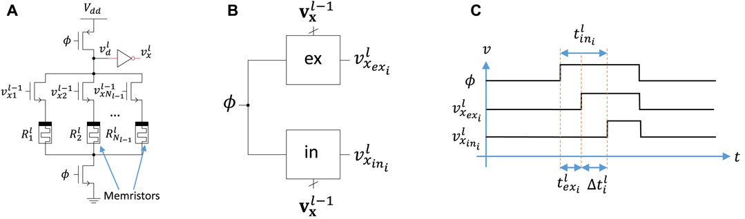
FIGURE 1. (A) Domino logic-style neuron circuit schematic. (B) Two domino circuits (ex and in) enable both positive and negative weights. (C) Information is encoded as the time difference between the excitatory and inhibitory rising edges.

We use a simple parasitic model for the capacitance in (Eq. 4), where each 1T1R synapse contributes one unit of capacitance C to the dynamic node from the NMOS drain. Assuming the PMOS transistor has minimal sizing, and the inverter has 2:1 PMOS:NMOS sizes ration, the total capacitance is estimated as

$C_d=\left(4+N_{l-1}\right)C=\left(4+N_{l-1}\right)A_{min}\frac{k_{ox}{ϵ}_0}{t_{ox}},(6)$

where A_min is the minimum transistor area, k_ox is the relative permittivity of SiO₂, ϵ₀ is the permittivity of free space, and t_ox is the transistor gate oxide thickness. Bounds on the time that it takes to discharge the dynamic node to the inverter threshold will be important to set an appropriate clock frequency. From (Eqs. 4–6), the minimum discharge time will be

$t_{min}^l=-\ln \left(\frac{\theta }{V_{dd}}\right)\frac{\left(4+N_{l-1}\right)C}{N_{l-1}{G}_{min}}=\frac{\beta }{N_{l-1}{G}_{min}}(7)$

where θ is the threhold voltage of the inverter.

Notice that this expression is approximately independent of N_l−1 as N_l−1 becomes large, meaning that these neurons are self-normalizing. That is, the maximum excitability of a neuron from the activity of one-presynptic neuron is constant regardless of fan-in. In contrast to the minimum discharge time, the maximum time will be infinite if we ignore leakage through selector transistors. However, we need to ensure that the dynamic node does not take longer to discharge than the evaluation period. Otherwise, there will be information lost. Therefore, we set a bound on the bias, which corresponds to a 1T1R cell that has a constant gate voltage of V_dd:

$G_{i0}^l\ge \frac{\beta }{T/2},(8)$

where T is the clock period. This ensures that $t_{max}^l=T/2$.

Figure 2 shows how the leakage current could affect the neuron behavior with increasing numbers of synapses. Here, we assume all of the synapse transistors are off, and each of the conductances is set to the maximum value, which will maximize the leakage current. The plot shows the final voltage on the dynamic node during a 50 ns evaluation period. As the number of synaptic input increases, both the capacitance on the dynamic node and the total leakage current increase. This has the effect of maintaining a relatively large voltage on the dynamic node, even with a large synaptic fan-in. In fact, as the number of synapses becomes large, the increased capacitance dominates, causing the effect of leakage to decrease. In all cases tested, the leakage current was not enough to discharge the dynamic node to the inverter’s threshold.

FIGURE 2

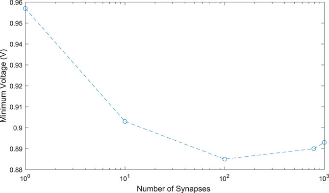
FIGURE 2. Effect of leakage current on the dynamic node versus the number of synaptic inputs.

To represent positive and negative weights, two of domino logic style neurons are used, inhibitory neuron to represent negative weight components and excitatory neuron to represent positive weight components as shown in Figure 1B. The time difference between nodes (inhibitory and excitatory) to reach the threshold of the inverter can be given as:

$\mathrm{\Delta }{t}_i^l=t_{e{x}_i}^l-t_{i{n}_i}^l=\beta V_{dd}\left(\frac{1}{{\mathbf{v}}_{\mathbf{x}}^{l-1}\cdot {\mathbf{G}}_{e{x}_i}^l}-\frac{1}{{\mathbf{v}}_{\mathbf{x}}^{l-1}\cdot {\mathbf{G}}_{i{n}_i}^l}\right)(9)$

This time difference encodes the input to the neuron’s binary activation function. Figure 1C shows an example where the excitatory domino circuit discharges faster than the inhibitory, leading to a positive value of Δt.

In this paper, we are interested in binary neurons, so it will be sufficient to know if $\mathrm{\Delta }{t}_i^l$ is negative or positive, which can be calculated using an arbiter circuit, the details of which are discussed later. First, though, it is important to point out how (Eq. 9) corresponds to pre-synaptic neuron outputs, weights, and the post-synaptic neuron inputs. The neuron input is $\mathrm{\Delta }{t}_i^l$, and we define the unitless version of it as $s_i^l=\mathrm{\Delta }{t}_i^l/(T/2)\in [-\mathrm{1,1}]$. The vector of pre-synaptic neuron outputs are ${\mathbf{v}}_{\mathbf{x}}^{l-1}$, and the unitless version is ${\mathbf{x}}^{l-1}={\mathbf{v}}_{\mathbf{x}}^{l-1}/V_{dd}\in [\mathrm{0,1}]$. Finally, the weights are related to the conductances ${\mathbf{G}}_{e{x}_i}^l$ and ${\mathbf{G}}_{i{n}_i}^l$. There are infinite ways to map a weight $w_{ij}^l$ to two conductances $G_{e{x}_{ij}}^l$ and $G_{i{n}_{ij}}^l$. In this work, we use a power optimized scheme, where minimum conductance values are used for the excitatory component and inhibitory component when the weights are negative and positive, respectively. Then, a linear function maps the opposite component:

$G_{e{x}_{ij}}^l=G_{min}+\left(G_{max}-G_{min}\right)\mathrm{m}\mathrm{a}\mathrm{x}\left(0,w_{ij}^l\right)(10)$

$G_{i{n}_{ij}}^l=G_{min}-\left(G_{max}-G_{min}\right)\mathrm{m}\mathrm{i}\mathrm{n}\left(0,w_{ij}^l\right)(11)$

Now, (Eq. 9) can be rewritten completely in terms of unitless values as:

$s_i^l={\beta }^{\prime }\left(\frac{1}{{\mathbf{x}}^{l-1}\cdot {\mathbf{w}}_{e{x}_i}^l}-\frac{1}{{\mathbf{x}}^{l-1}\cdot {\mathbf{w}}_{i{n}_i}^l}\right)(12)$

where ${\mathbf{w}}_{e{x}_i}^l={\mathbf{G}}_{e{x}_i}^l/G_{max}$ and ${\mathbf{w}}_{i{n}_i}^l={\mathbf{G}}_{i{n}_i}^l/G_{max}$, and β′ = 2β/(TG_max). Contrast this with the usual dot product input of a neural network:

$s_i^l={\mathbf{x}}^{l-1}\cdot {\mathbf{w}}_i^l(13)$

In other words, the neuron input of our design has a non-linear relationship with pre-synaptic neuron outputs and the weights, whereas typical formulations of neural networks have a linear relationship. This non-linearity stems from the natural non-linearity of RC circuits, and to remove it would require an additional evaluation phase, such as the method proposed in Bavandpour et al. (2019). Instead, we opt to keep the hardware as simple as possible and we note that the non-linearity could be accounted for in two ways. On one hand, the behavior of (Eq. 12) could be modeled directly in Tensorflow. While this would be the simplest solution, we have found that this leads to several simulation challenges. For example, it is easy for (Eq. 12) to have undefined values when inputs or weights become small. In addition, we observed unstable learning and, in some cases, inability to converge when working directly with (Eq. 12).

Interestingly, though, because our neurons are binary, only the sign of $s_i^l$ is important, and we can use (Eq. 13) for training. Figure 3 compares the values in (Eq. 9), (Eq. 12), and (Eq. 13). Here, we performed 1000 Monte Carlo simulations with uniformly-distributed weights between −1 and 1, and Bernoulli-distributed inputs with probability value 0.5. From the plot, one can observe that the normal dot product operation in (Eq. 13), which we refer to as “software” maps non-linearly to the excitatory-inhibitory time difference as well as the normalized version of the time difference, referred to as “hardware”. The ranges of the hardware values are inversely proportional to the ranges of the software values, which is expected due to the inverse relationships in (Eq. 9) and (Eq. 12). Critically, all of the datapoints are in the lower-left and upper-right quadrants, meaning that the sign of the software and hardware data are always the same. In other words, the non-linear behavior of the neuron’s input will not affect its output. The next section discusses how this sign is captured using an arbiter to yield a binary activation function.

FIGURE 3

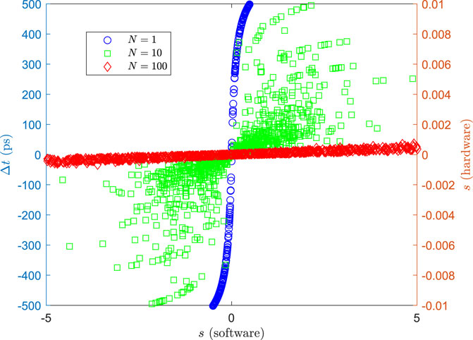
FIGURE 3. Time difference between excitatory and inhibitory domino circuits (Eq. 9) and unitless neuron input (Eq. 12) vs. a normal dot product input (Eq. 13).

3.2 Arbiter design and placement

We explored two possible designs for implementing the arbiter-based activation function that converts the time difference between the excitatory and inhibitory domino circuits into a binary value:

$v_{x_i}^l=\left\{\begin{array}{cc}0,\hfill & \hfill \mathrm{\Delta }{t}_i^l\le 0\\ V_{dd},\hfill & \hfill \mathrm{\Delta }{t}_i^l>0\end{array}\right.(14)$

Initially, we designed the arbiter as shown in Figure 4A. Here, NOR gates are used to disable the inhibitory (excitatory) circuit from discharging once the excitatory (inhibitory) circuit crosses the inverter threshold. An advantage of this approach is that only one of the domino circuits will fully discharge. For example, if the excitatory domino circuit discharges more quickly, it will cause the inhibitory circuit to go back into the pre-charge phase before it reaches the inverter threshold. This will reduce dynamic power consumed during the pre-charge phase. However, we observed that this approach has poor stability (seen in the waveform in Figure 4A especially for small Δt, and often led to oscillations as well as incorrect outputs.

FIGURE 4

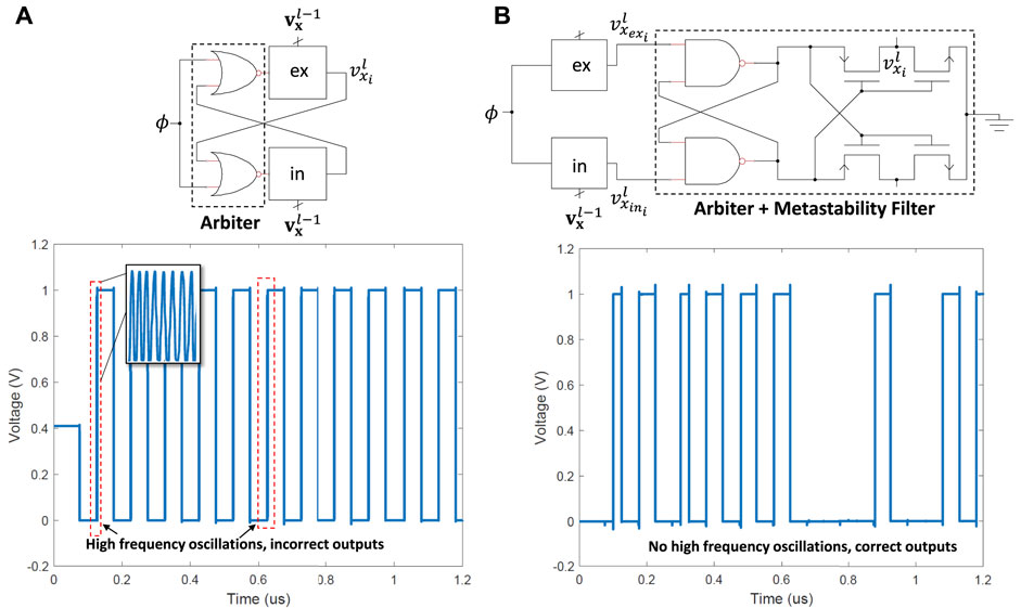
FIGURE 4. (A) Domino logic style neuron with NOR gate as an arbiter, showing oscillatory behavior at the output node due to unstable feedback. (B) Simplification of domino logic style neuron with NAND gate-based arbiter, which eliminates oscillatory behavior.

The second design is shown in Figure 4B, which uses cross-coupled NAND gates and includes a metastability filter to ensure the output doesn’t remain long in an invalid logic state and consequently, it is possible for that design to have that behaviour and enter metastability. In addition, NOR gate two large PMOS transistors in series, which means more capacitance and more delay compared to the NAND gate. The main advantage of this design is that the memristor domino circuits are not included in the feedback path, so the circuit’s stability is not dependent on the memristor states. This is the design that we used for the rest of this paper.

3.3 Synchronization strategy

In order to implement large multi-layer neural networks information from one layer needs to be transferred to the next layer. Synchronizing the transfer of information between layers is critical, and here we explore three techniques with various tradeoffs. In this section, we use the XOR problem as a case study, where our multi-layer perceptron (MLP) neural network consists of 2 inputs, 2 hidden neurons, and 1 output. The output should be ‘0’ when both inputs are the same and ‘1’ when the inputs are different.

3.3.1 Method 1: Multiple clocks with different duty cycles

The simplest synchronization strategy employs one clock per layer as shown in Figure 5. Notice that the neuron and synapse designs discussed earlier are easily integrated into a crossbar-like circuit for efficient implementation. Here, three clocks are used, corresponding to the input (Clk), hidden layer (Clk-1), and output layer (Clk-2). The inputs are Vxex1-1 and Vxex2-1 and the final output is output. For a given input, first all clocks are ‘0’ to pre-charge all domino circuits. Then, Clk becomes ‘1’ for input evaluation, enabling the input to be forwarded to the hidden layer. Then, the clocks of each layer transition to ‘1’ one-at-a-time and remain at ‘1’ until all layers have been evaluated. This technique has no sequencing overhead. However, the disadvantage of this technique is that each layer has to wait for all of the previous layers to finish before it performs any evaluation. Generally, the cycle time is the sum of logic delay and sequencing over head. The logic delay depends on the discharging rate of the pull down network which mainly depends on the memristor state during the evaluation phase.

FIGURE 5

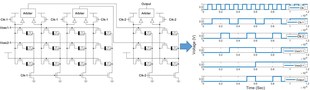
FIGURE 5. The MLP schematic and simulation for the XOR problem using multiple overlapping clocks with different duty cycles.

3.3.2 Method 2: Flip-flop pipelining

The throughput of the design can be improved using conventional pipelining with flip-flips, shown in Figure 6. Here, a single clock Clk controls D flip-flops between layers, which hold evaluation results from the previous layer until the subsequent layer completes its evaluation. This is the classical clocking strategy and has been widely used due to its robustness. In this method, the entire network can be pipelined across layers and each neuron can perform evaluations on every clock cycle. The disadvantage of this approach is the sequencing overhead (time and area) of the flip-flop.

FIGURE 6

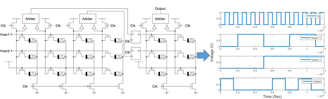
FIGURE 6. The MLP schematic and simulation for the XOR problem using multiple overlapping clocks with conventional pipelining based on D flip-flops.

3.3.3 Method 3: Dynamic pipelining

If clocks are overlapped, flip-flops could be eliminated and this is the third approach that is called the skew tolerant domino (Harris and Horowitz, 1997), shown in Figure 7. The idea is that the overlapping clocks ensure that the evaluation of a neuron in the subsequent layer has enough time to evaluate before the previous layer neurons starts their pre-charging phase. Here, three overlapped clocks, Clk-0, Clk-1, and Clk-2 are used for the input, hidden, and output layers, repsectively. These clocks can be generate using simple delay circuits based on, e.g. inverter chains. When the previous layer neurons starts their pre-charging phase, the dynamic gates will pre-charged to V_dd and therefore the static gates will be discharged to ground. This means that the input to the subsequent layer falls low, seemingly violating the monotonicity rule. The monotonicity rule states that inputs to dynamic gates must make only low to high transitions while the gates are in the evaluation phase. However, the domino logic in the subsequent layer will remain at whatever value it evaluated based on the results of the first layer when its inputs fall low because both the pull-down transistors and the pre-charge transistor will be off (Harris and Horowitz, 1997). Therefore, the neurons will keep their value even when previous layer pre-charges. Hence, there is no need for a latch or a flip-flop. This method has improved throughput over the multiple duty cycle method, but does not have the flip-flop area overhead associated with conventional pipelining. The rest of our simulations are based on this technique.

FIGURE 7

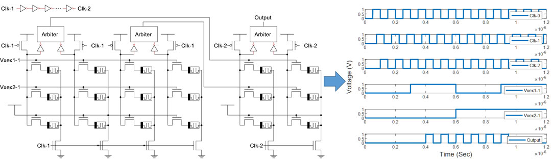
FIGURE 7. The MLP schematic and simulation for the XOR problem using skew-tolerant dynamic pipelining.

4 Noise modeling

A key component of our design is the arbiter-based binary activation function. Arbiters are essential parts of many digital and mixed-signal designs such as memories and microprocessors (Kim and Dutton, 1990). However, these circuits could cause system failure due to metastability issues. In the proposed circuit, there will be stochastic behaviour of the neuron’s output for small differences in arrival times of the edge of the excitatory and inhibitory signals at the arbiter’s inputs. In particular, when the value of Δt is close to the arbiter’s aperture time (measured to be approximately 2 ps), it may enter a metastable state. Combined with noise, the metastable state will stochastically resolve to either ‘0’ or ‘1.’ Figure 8A shows the distribution of Δt for hidden layer neurons in an MLP network that we trained to classify handwritten digits from the MNIST dataset. The hidden is relatively small, with only 100 neurons, so the network does not give good accuracy. However, the point here is to show the distribution, which is approximately normal. This is expected, since trained neural networks will tend to have normally-distributed weights, so the dot product of pre-synaptic neuron outputs with post-synaptic neuron weight vectors will also be normally distributed. In this case, the mean is around 100 ps, but for other datasets and network sizes, the mean may be centered closer to 0 or at a negative value. In fact, as the size of the layer increases, it is expected that the mean will be closer to 0. This means, that arbiter inputs may often be within the aperture window, potentially leading to stochastic behavior. Figure 8B shows a Monte Carlo simulation of the arbiter output for a small Δt in the presence of noise. Here, the Δt is positive, and should result in an output of ‘1’ but in many samples, the arbiter output is ‘0’. Figure 9 shows a box plot of the mismatched neuron outputs between an ideal software simulation, where noise is not considered, and a hardware simulation with different levels of noise for the MNIST dataset. In this case, to keep the simulation tractable, the network only has 10 hidden neurons, and already there are some mismatched neuron outputs.

FIGURE 8

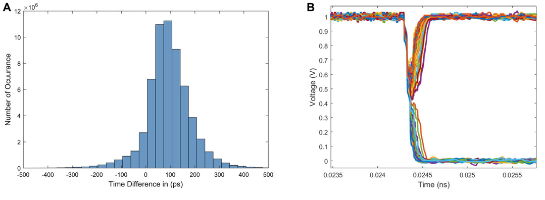
FIGURE 8. (A) Distribution of Δt across 100 hidden neurons for 60,000 handwritten digit inputs. (B) Arbiter output for small Δt value in the presence of noise.

FIGURE 9

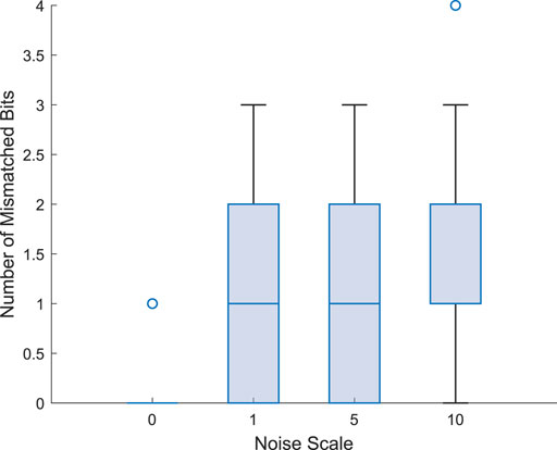
FIGURE 9. The mismatched bits with different levels of noise.

To capture this behavior, we developed a simple stochastic model of the arbiter by simulating its behavior with different levels of transient noise (low, moderate, and high). The inputs to the arbiter are the time difference Δt between the excitatory and inhibitory signals. These two signals are swept from −10 ps to 10 ps. The simulations were performed 100 times for each run, and the neuron’s output probability was calculated after. The results are shown in Figure 10A. The data are fit to a sigmoid function:

$\frac{a}{1+\exp \left(-bx\right)}(15)$

where a and b are the fitting parameters for sigmoid function. For low noise: a = 99.93, b = 7.394. For moderate noise: a = 99.59, b = 2.681. For high noise: a = 98.77, b = 1.119. Note that other sources of noise such as process variations will also contribute to changes in the neuron probability for small differences in Δt. For example, consider Figure 10B, which shows the simulation of the arbiter under different process CMOS process corners. The overall effect of the different corners is to modify the slope of the sigmoid curve. Qualitatively similar behavior also results from variations in voltage and temperature.

FIGURE 10

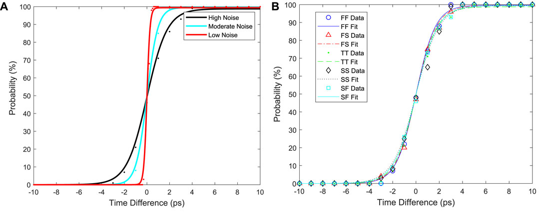
FIGURE 10. (A) The probability of a neuron’s output being equal to ‘1’ as a function of input time difference between excitatory and inhibitory domino circuits. (B) The effect of process variations on the neuron’s output probability for the high noise case.

5 Results and analysis

5.1 Simulation approach

Simulation of large neural networks in electronic solvers like SPICE is prohibitively slow. We use a combination of SPICE (Synopsys HSPICE) and Tensorflow in order to have fast simulations while still capturing key hardware behavior. Our simulation strategy is shown in Figure 11. The key aspects of the circuit behavior discussed in the previous sections have been captured using HSPICE simulations with a predictive technology 130 nm bulk CMOS transistor model (https://ptm.asu.edu/) and memristor parameters based on the memristor proposed in (Prezioso et al., 2015), which has ON and OFF conductance values of G_min = 5 × 10⁻⁷ and G_max = 5 × 10⁻⁵ and programming voltage magnitudes near 1 V. In this work, only a subset of the device conductance range is used: G_min = 1 × 10⁻⁶ S and G_max = 1 × 10⁻⁵ S. Since the device has approximately linear behavior at low voltages that are below the programming threshold, we have modeled it as a resistor. Tensorflow is used to train the neural network to get the weights, which are converted into conductances based on the weight mapping in (Eq. 10) and (Eq. 11). Finally, another Tensorflow model with identical neural network topology but more accurate hardware behavior (e.g., stochastic behavior of neurons, conductance-based weights, etc.) is used to estimate the hardware performance on the dataset.

FIGURE 11

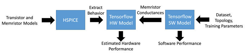
FIGURE 11. Simulation strategy used in this work, which combines SPICE-level simulation with Tensorflow neural network simulation.

5.2 Performance on the MNIST dataset

We tested the proposed design approach for an MLP with 1000 hidden neurons on the MNIST handwritten digit dataset (http://yann.lecun.com/exdb/mnist/). The results are shown in Figure 12A. Without considering noise, the software and hardware simulations produce almost identical results, with accuracies in the high 90s. These accuracies hold approximately constant across different levels of weight precision, from 3 to 10 bits. Note that 1- and 2-bit precision results were much lower and are not included in the plot. As noise effects are added to the simulation, the accuracy generally decreases. Low and moderate noise results are almost identical, while high noise gives a clear drop in accuracy. However, even with high noise magnitude, the degradation is less than 2%. We have also explored the effects of conductance variations on the proposed hardware design. These variations may arise from imprecise programming or drift of conductance values over time. Small conductance variations (e.g., 10%) have negligible effects on the test accuracy while larger variations (20% and more) can start to have considerable effects. Note that the effects of conductance variations are more pronounced at higher levels of weight precisions, which may motivate employing lower-precision devices or fewer of devices’ conductance levels.

FIGURE 12

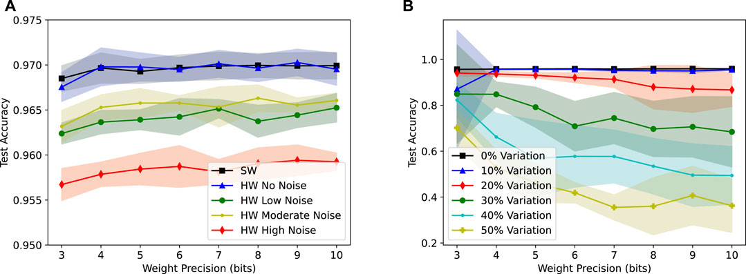
FIGURE 12. (A) Test accuracy of the software and proposed hardware implementations of an MLP with 1000 hidden neurons on the MNIST varying levels of noise. (B) Test accuracy of the hardware under varying levels of conductance variations.

5.3 Power analysis and comparison with other works

The power consumption of the proposed design was modeled by assuming that most of the power is consumed when a neuron pre-charges. The justification for this is that, especially for neurons with high fan-in the switching capacitance of the neuron’s dynamic node will be much larger than the capacitance at other nodes in the circuit. Therefore, the power can be formulated as

$P\approx 3\times \left(1+\eta \right){\displaystyle \sum _{l=2}^L}\alpha C^l{V}_{dd}^{2}f(16)$

where η is a fitting parameter that comes from the extra power associated with the inverter, arbiter, etc., α is the switching activity factor, L is the number of layers, and C^l is the total switching capacitance of the layer. For the dynamic pipelining synchronization scheme, α = 1, since each layer will pre-charge every clock cycle. In addition, the value of C^l is 3C times twice the number of synapses in a the layer (to account for both excitatory and inhibitory). The factor of 3 comes from each synapse’s source, drain, and memristor capacitance. We have empirically found η ≈ 0.19. In Figure 13, we show the power consumption for 100 randomly-sized 3-layer networks vs. the number of synapses and neurons in the network. For each network, both the inputs and weights were generated randomly. Furthermore, the network used a clock frequency of 10 MHz. From this data, we estimate the energy efficiency of our design to be approximately 1.26 fJ per classification per synapse. A comparison with similar works that designed MLPs for MNIST classification is shown in Table 1. Our work has slightly better energy efficiency than that reported in Yakopcic et al. (2015) while giving much better accuracy. 2T2R are needed to represent positive and negative weights. For our work, the number of transistors per neuron is 20. For Yakopcic et al. (2015) we estimate the number of transistors per neuron to be 4, and the number of transistors per neuron in (Jiang et al., 2018) is 30 (15 for excitatory and 15 for inhibitory).

FIGURE 13

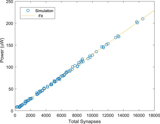
FIGURE 13. Power consumption vs. total number of synapses for the proposed design.

TABLE 1

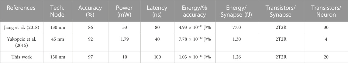
TABLE 1. Comparison of memristor-based neuromorphic designs on MNIST classification.

6 Conclusion and future work

This paper presented a novel architecture for memristor-based neuromorphic computing using domino logic. The key behavioral elements of the hardware, including noise-induced stochasticity, were captured in behavioral simulations using Tensorflow, and the design was analyzed on an MNIST classification task. Results indicate that the proposed design has slightly better energy efficiency (1.26 fJ/synapse) than competing approaches while providing much higher accuracy (97%). Possible avenues for future work include design of on-chip training circuitry and further energy reduction using additional low-power design techniques.

Data availability statement

The original contributions presented in the study are included in the article/supplementary material, further inquiries can be directed to the corresponding author.

Author contributions

HH helped design all circuits, carried out all simulations, analyzed the data, and wrote the manuscript. CM conceived the domino logic design idea, helped design all circuits, wrote the manuscript, and supervised the study.

Funding

Funding for this work was provided by the Rochester Institute of Technology Computer Engineering Department.

Conflict of interest

The authors declare that the research was conducted in the absence of any commercial or financial relationships that could be construed as a potential conflict of interest.

Publisher’s note

All claims expressed in this article are solely those of the authors and do not necessarily represent those of their affiliated organizations, or those of the publisher, the editors and the reviewers. Any product that may be evaluated in this article, or claim that may be made by its manufacturer, is not guaranteed or endorsed by the publisher.

References

Bavandpour, M., Sahay, S., Mahmoodi, M. R., and Strukov, D. (2019). Efficient mixed-signal neurocomputing via successive integration and rescaling. IEEE Trans. Very Large Scale Integration Syst. 28, 823–827. doi:10.1109/tvlsi.2019.2946516

CrossRef Full Text | Google Scholar

Chen, A. (2016). A review of emerging non-volatile memory (nvm) technologies and applications. Solid-State Electron. 125, 25–38. doi:10.1016/j.sse.2016.07.006

CrossRef Full Text | Google Scholar

Chua, L. (2014). If it’s pinched it’sa memristor. Semicond. Sci. Technol. 29, 104001. doi:10.1088/0268-1242/29/10/104001

CrossRef Full Text | Google Scholar

Dahl, G. E., Yu, D., Deng, L., and Acero, A. (2011). Context-dependent pre-trained deep neural networks for large-vocabulary speech recognition. IEEE Trans. audio, speech, Lang. Process. 20, 30–42. doi:10.1109/tasl.2011.2134090

CrossRef Full Text | Google Scholar

Davies, M., Srinivasa, N., Lin, T.-H., Chinya, G., Cao, Y., Choday, S. H., et al. (2018). Loihi: A neuromorphic manycore processor with on-chip learning. Ieee Micro 38, 82–99. doi:10.1109/mm.2018.112130359

CrossRef Full Text | Google Scholar

Douglas, R., Mahowald, M., and Mead, C. (1995). Neuromorphic analogue vlsi. Annu. Rev. Neurosci. 18, 255–281. doi:10.1146/annurev.ne.18.030195.001351

PubMed Abstract | CrossRef Full Text | Google Scholar

Everson, L. R., Liu, M., Pande, N., and Kim, C. H. (2018). “A 104.8 tops/w one-shot time-based neuromorphic chip employing dynamic threshold error correction in 65nm,” in 2018 IEEE Asian Solid-State Circuits Conference (A-SSCC) (Tainan, Taiwan: IEEE), 273–276. doi:10.1109/ASSCC.2018.8579302

CrossRef Full Text | Google Scholar

Freye, F., Lou, J., Bengel, C., Menzel, S., Wiefels, S., and Gemmeke, T. (2022). Memristive devices for time domain compute-in-memory. IEEE J. Explor. Solid-State Comput. Devices Circuits 8, 119–127. doi:10.1109/jxcdc.2022.3217098

CrossRef Full Text | Google Scholar

Harris, D., and Horowitz, M. A. (1997). Skew-tolerant domino circuits. IEEE J. Solid-State Circuits 32, 1702–1711. doi:10.1109/4.641690

CrossRef Full Text | Google Scholar

Hendy, H., and Merkel, C. (2022). Review of spike-based neuromorphic computing for brain-inspired vision: Biology, algorithms, and hardware. J. Electron. Imaging 31, 010901. doi:10.1117/1.jei.31.1.010901

CrossRef Full Text | Google Scholar

Hubara, I., Courbariaux, M., Soudry, D., El-Yaniv, R., and Bengio, Y. (2017). Quantized neural networks: Training neural networks with low precision weights and activations. J. Mach. Learn. Res. 18, 6869–6898.

Google Scholar

Jiang, H., Yamada, K., Ren, Z., Kwok, T., Luo, F., Yang, Q., et al. (2018). “Pulse-width modulation based dot-product engine for neuromorphic computing system using memristor crossbar array,” in 2018 IEEE International Symposium on Circuits and Systems (ISCAS) (Florence, Italy: IEEE), 1–4. doi:10.1109/ISCAS.2018.8351276

CrossRef Full Text | Google Scholar

Jouppi, N. P., Young, C., Patil, N., Patterson, D., Agrawal, G., Bajwa, R., et al. (2017). “In-datacenter performance analysis of a tensor processing unit,” in Proceedings of the 44th annual international symposium on computer architecture (Toronto, ON, Canada: IEEE), 1–12. doi:10.1145/3079856.3080246

CrossRef Full Text | Google Scholar

Kim, L.-S., and Dutton, R. W. (1990). Metastability of cmos latch/flip-flop. IEEE J. solid-state circuits 25, 942–951. doi:10.1109/4.58286

CrossRef Full Text | Google Scholar

Lee, E. H., and Wong, S. S. (2016). Analysis and design of a passive switched-capacitor matrix multiplier for approximate computing. IEEE J. Solid-State Circuits 52, 261–271. doi:10.1109/jssc.2016.2599536

CrossRef Full Text | Google Scholar

Marinella, M. J., Agarwal, S., Hsia, A., Richter, I., Jacobs-Gedrim, R., Niroula, J., et al. (2018). Multiscale co-design analysis of energy, latency, area, and accuracy of a reram analog neural training accelerator. IEEE J. Emerg. Sel. Top. Circuits Syst. 8, 86–101. doi:10.1109/jetcas.2018.2796379

CrossRef Full Text | Google Scholar

Merkel, C. (2019). “Current-mode memristor crossbars for neuromorphic computing,” in Proceedings of the 7th Annual Neuro-inspired Computational Elements Workshop, 1–6. doi:10.1145/3320288.3320298

CrossRef Full Text | Google Scholar

Merkel, C., and Kudithipudi, D. (2017). “Neuromemristive systems: A circuit design perspective,” in Advances in neuromorphic hardware exploiting emerging nanoscale devices. Cognitive systems monographs. Editor M. Suri (New Delhi: Springer), Vol. 31, 45–64. doi:10.1007/978-81-322-3703-7_3

CrossRef Full Text | Google Scholar

Nandakumar, S., Kulkarni, S. R., Babu, A. V., and Rajendran, B. (2018). Building brain-inspired computing systems: Examining the role of nanoscale devices. IEEE Nanotechnol. Mag. 12, 19–35. doi:10.1109/mnano.2018.2845078

CrossRef Full Text | Google Scholar

Prezioso, M., Merrikh-Bayat, F., Hoskins, B., Adam, G. C., Likharev, K. K., and Strukov, D. B. (2015). Training and operation of an integrated neuromorphic network based on metal-oxide memristors. Nature 521, 61–64. doi:10.1038/nature14441

PubMed Abstract | CrossRef Full Text | Google Scholar

Rueckauer, B., Lungu, I.-A., Hu, Y., Pfeiffer, M., and Liu, S.-C. (2017). Conversion of continuous-valued deep networks to efficient event-driven networks for image classification. Front. Neurosci. 11, 682. doi:10.3389/fnins.2017.00682

PubMed Abstract | CrossRef Full Text | Google Scholar

Sahay, S., Bavandpour, M., Mahmoodi, M. R., and Strukov, D. (2020). Energy-efficient moderate precision time-domain mixed-signal vector-by-matrix multiplier exploiting 1t-1r arrays. IEEE J. Explor. Solid-State Comput. Devices Circuits 6, 18–26. doi:10.1109/jxcdc.2020.2981048

CrossRef Full Text | Google Scholar

Schuman, C. D., Potok, T. E., Patton, R. M., Birdwell, J. D., Dean, M. E., Rose, G. S., et al. (2017). A survey of neuromorphic computing and neural networks in hardware. arXiv preprint arXiv:1705.06963.

Google Scholar

Seide, F., Li, G., and Yu, D. (2011). “Conversational speech transcription using context-dependent deep neural networks,” in Twelfth annual conference of the international speech communication association. doi:10.5555/3042573.3042574

CrossRef Full Text | Google Scholar

Sinangil, M. E., Erbagci, B., Naous, R., Akarvardar, K., Sun, D., Khwa, W.-S., et al. (2020). A 7-nm compute-in-memory sram macro supporting multi-bit input, weight and output and achieving 351 tops/w and 372.4 gops. IEEE J. Solid-State Circuits 56, 188–198. doi:10.1109/jssc.2020.3031290

CrossRef Full Text | Google Scholar

Sung, C., Hwang, H., and Yoo, I. K. (2018). Perspective: A review on memristive hardware for neuromorphic computation. J. Appl. Phys. 124, 151903. doi:10.1063/1.5037835

CrossRef Full Text | Google Scholar

Yakopcic, C., Hasan, R., and Taha, T. M. (2015). “Memristor based neuromorphic circuit for ex-situ training of multi-layer neural network algorithms,” in 2015 International Joint Conference on Neural Networks (IJCNN) (Killarney, Ireland: IEEE), 1–7. doi:10.1109/IJCNN.2015.7280813

CrossRef Full Text | Google Scholar