A Lyapunov-Stable Adaptive Method to Approximate Sensorimotor Models for Sensor-Based Control

1. Introduction

Robots are widely used in industry to perform a myriad of sensor-based applications ranging from visually servoed pick-and-place tasks to force-regulated workpiece assemblies (Nof, 1999). Their accurate operation is largely due to the fact that industrial robots rely on fixed settings that enable the exact characterization of the tasks' sensorimotor model. Although this full characterization requirement is fairly acceptable in industrial environments, it is too stringent for many service applications where the mechanical, perceptual and environment conditions are not exactly known or might suddenly change (Navarro-Alarcon et al., 2019), e.g., in domestic robotics (where environments are highly dynamic), field robotics (where variable morphologies are needed to navigate complex workspaces), autonomous systems (where robots must adapt and operate after malfunctions), to name a few cases.

In contrast to industrial robots, the human brain has a high degree of adaptability that allows it to continuously learn sensorimotor relations. The brain can seemingly coordinate the body (whose morphology persistently changes throughout life) under multiple circumstances: severe injuries, amputations, manipulating tools, using prosthetics, etc. It can also recalibrate corrupted or modified perceptual systems: a classical example is the manipulation experiment performed in Kohler (1962) with image inverting goggles that altered a subject's visual system. In infants, motor babbling is used for obtaining (partly from scratch and partly innate) a coarse sensorimotor model that is gradually refined with repetitions (Von Hofsten, 1982). Providing robots with similar incremental and life-long adaptation capabilities is precisely our goal in this paper.

From an automatic control point of view, a sensorimotor model is needed for coordinating input motions of a mechanism with output sensor signals (Huang and Lin, 1994), e.g., controlling the shape of a manipulated soft object based on vision (Navarro-Alarcon et al., 2016) or controlling the balance of a walking machine based on a gyroscope (Yu et al., 2018). In the visual servoing literature, the model is typically represented by the so-called interaction matrix (Hutchinson et al., 1996; Cherubini et al., 2015), which is computed based on kinematic relations between the robot's configuration and the camera's image projections. In the general case, sensorimotor models depend on the physics involved in constructing the output sensory signal; If this information is uncertain (e.g., due to bending of robot links, repositioning of external sensors, deformation of objects), the robot may no longer properly coordinate actions with perception. Therefore, it is important to develop methods that can efficiently provide robots with the capability to adapt to unforeseen changes of the sensorimotor conditions.

Classical methods in robotics to compute this model (see Sigaud et al., 2011 for a review) can be roughly classified into structure-based and structure-free approaches (Navarro-Alarcon et al., 2019). The former category represents “calibration-like” techniques [e.g., off-line (Wei et al., 1986) or adaptive (Wang et al., 2008; Liu et al., 2013; Navarro-Alarcon et al., 2015)] that aim to identify the unknown model parameters. These approaches are easy to implement, however, they require exact knowledge of the analytical structure of the sensory signal (which might not be available or subject to large uncertainties). Also, since the resulting model is fixed to the mechanical/perceptual/environmental setup that was used for computing it, these methods are not robust to unforeseen changes.

For the latter (structure-free) category, we can further distinguish between two main types (Navarro-Alarcon et al., 2019): instantaneous and distributed estimation. The first type performs online numerical approximations of the unknown model (whose structure does not need to be known); Some common implementations include e.g., Broyden-like methods (Hosoda and Asada, 1994; Jagersand et al., 1997; Alambeigi et al., 2018) and iterative gradient descent rules (Navarro-Alarcon et al., 2015; Yip et al., 2017). These methods are robust to sudden configuration changes, yet, as the sensorimotor mappings are continuously updated, they do not preserve knowledge of previous estimations (i.e., it's model is only valid for the current local configuration). The second type distributes the estimation problem amongst multiple computing units; The most common implementation is based on (highly nonlinear) connectionists architectures (Li and Cheah, 2014; Lyu and Cheah, 2018; Hu et al., 2019). These approaches require very large amounts of training data to properly constrain the learning algorithm, which is impractical in many situations. Other distributed implementations (based on SOM-like sensorimotor “patches,” Kohonen, 2013) are reported e.g., in Zahra and Navarro-Alarcon (2019), Pierris and Dahl (2017), and Escobar-Juarez et al. (2016), yet, the stability properties of its algorithms are not rigorously analyzed.

As a solution to these issues, in this paper we propose a new approach that approximates unknown sensorimotor models based on local data observations only. In contrast to previous state-of-the-art methods, our adaptive algorithm has the following original features:

• It requires few data observations to train and constrain the algorithm (which allows to implement it in real-time).

• The number of minimum data points to train it can be analytically obtained (which makes data collection more effective).

• The stability of its update rule can be rigorously proved (which enables to deterministically predict its performance).

The proposed method is general enough to be used with different types of sensor signals and robot mechanisms.

The rest of the manuscript is organized as follows: section 2 presents preliminaries, section 3 describes the proposed method, section 4 reports the conducted numerical study, and section 5 gives final conclusions.

2. Preliminaries

2.1. Notation

Along this note we use very standard notation. Column vectors are denoted with bold small letters m and matrices with bold capital letters M. Time evolving variables are represented as m_t, where the subscript ∗_t denotes the discrete time instant. Gradients of functions $b=\beta (\text{m}):{M}\mapsto {B}$ are denoted as ∇β(m) = (∂β/∂m)^⊺.

2.2. Configuration Dependant Feedback

Consider a fully-actuated robotic system whose instantaneous configuration vector (modeling e.g., end-effector positions in a manipulator, orientation in a robot head, etc.) is denoted by the vector ${\text{x}}_t\in {ℝ}^n$. Such model can only be used to represent traditional rigid systems, thus, it excludes soft/continuum mechanisms (Falkenhahn et al., 2015) or robots driven by elastic actuators (Wang et al., 2016). Without loss of generality, we assume that its coordinates are all represented using the same unitless range¹. To perform a task, the robot is equipped with a sensing system that continuously measure a physical quantity whose instantaneous values depend on x_t. Some examples of these types of configuration-dependent feedback signals are: geometric features in an image (Tirindelli et al., 2020), forces applied onto a compliant surface (Navarro-Alarcon et al., 2014; Bouyarmane et al., 2019), proximity to an object (Cherubini and Chaumette, 2013), intensity of an audio source (Magassouba et al., 2016), attitude of a balancing body (Defoort and Murakami, 2009), shape of a manipulated object (Navarro-Alarcon and Liu, 2018), temperature from a heat source (Saponaro et al., 2015), etc.

Let ${\text{y}}_t\in {ℝ}^m$ denote the vector of feedback features that quantify the task; Its coordinates might be constructed with raw measurements or be the result of some processing. We model the instantaneous relation between this sensor signal and the robot's configuration as (Chaumette and Hutchinson, 2006):

$\begin{array}{ll}{\text{y}}_t=f({\text{x}}_t):{ℝ}^n\mapsto {ℝ}^m& (1)\end{array}$

Remark 1. Along this paper, we assume that the feedback feature functional f(x_t) is smooth (at least twice differentiable) and its Jacobian matrix has a full row/column rank (which guarantees the existence of its (pseudo-)inverse).

2.3. Uncalibrated Sensorimotor Control

In our formulation of the problem, it is assumed that the robotic system is controlled via a standard position/velocity interface (as in e.g., Whitney, 1969; Siciliano, 1990), a situation that closely models the majority of commercial robots. With position interfaces, the motor action ${\text{u}}_t\in {ℝ}^n$ represents the following displacement difference:

$\begin{array}{ll}{\text{x}}_{t+1}-{\text{x}}_t={\text{u}}_t& (2)\end{array}$

Such kinematic control interface renders the typical stiff behavior present in industrial robots (for this model, external forces do not affect the robot's trajectories). The methods in this paper are formulated using position commands, however, these can be easily transformed into robot velocities ${\text{v}}_t\in {ℝ}^n$ by dividing u_t by the servo controller's time step dt as follows u_t/dt = v_t.

The expression that describes how the motor actions result in changes of feedback features is represented by the first-order difference model²:

$\begin{array}{ll}{\text{y}}_{t+1}={\text{y}}_t+\text{A}({\text{x}}_t){\text{u}}_t={\text{y}}_t+{\delta }_t& (3)\end{array}$

where the configuration-dependent matrix $\text{A}({\text{x}}_t)=\partial f/\partial {\text{x}}_t\in {ℝ}^{m\times n}$ represents the traditional sensor Jacobian matrix of the system (also known as the interaction matrix in the visual servoing literature; Hutchinson et al., 1996). To simplify notation, throughout this paper we shall omit its dependency on x_t and denote it as A_t = A(x_t). The flow vector ${\delta }_t={\text{A}}_t{\text{u}}_t\in {ℝ}^m$ represents the sensor changes that result from the action u_t. Figure 1 conceptually depicts these quantities.

FIGURE 1

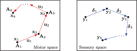
Figure 1. Representation of a configuration trajectory x_t, its associated transformation matrices A_t and motor actions u_t, that produce the measurements y_t and sensory changes δ_t.

The sensorimotor control problem consists in computing the necessary motor actions for the robot to achieve a desired sensor configuration. Without loss of generality, in this note, such configuration is characterized as the regulation of the feature vector y_t toward a constant target y^*. The necessary motor action to reach the target can be computed by minimizing the following quadratic cost function:

$\begin{array}{ll}J=\left|\right|\lambda sat({\text{y}}_t-{\text{y}}^{*})+{\text{A}}_t{\text{u}}_t|{|}^2& (4)\end{array}$

where λ > 0 is a gain and sat(·) a standard saturation function (defined as in e.g., Chang et al., 2018). The rationale behind the minimization of the cost (4) is to find an incremental motor command u_t that forward-projects into the sensory space (via the interaction matrix A_t) as a vector pointing toward the target y^*. By iteratively commanding these motions, the distance $\left|\right|{\text{y}}_t-{\text{y}}^{*}\left|\right|$ is expected to be asymptotically minimized.

To obtain u_t, let us first compute the extremum ∇J(u_t) = 0, which yields the normal equation

$\begin{array}{ll}{\text{A}}_t^{⊺}{\text{A}}_t{\text{u}}_t=-\lambda {\text{A}}_t^{⊺}sat({\text{y}}_t-{\text{y}}^{*})& (5)\end{array}$

Solving (5) for u_t, gives rise to the motor command that minimizes J:

$\begin{array}{ll}{\text{u}}_t=-\lambda {\text{A}}_t^{\#}sat({\text{y}}_t-{\text{y}}^{*})& (6)\end{array}$

where ${\text{A}}_t^{\#}\in {ℝ}^{n\times m}$ is a generalized pseudo-inverse matrix satisfying ${\text{A}}_t{\text{A}}_t^{\#}{\text{A}}_t={\text{A}}_t$ (Nakamura, 1991), whose existence is guaranteed as A_t has a full column/row rank (depending on whichever is larger n or m). Yet, note that for the case where m > n, the cost function J can only be locally minimized.

Note that the computation of (6) requires exact knowledge of A_t. To analytically calculate this matrix, we need to fully calibrate the system, which is too restrictive for applications where the sensorimotor model is unavailable or might suddenly change. This situation may happen if the mechanical structure of the robot is altered (e.g., due to bendings or damage of links), or the configuration of the perceptual system is changed (e.g., due to relocating external sensors), or the geometry of a manipulated object changes (e.g., due to grasping forces deforming a soft body), to name a few cases. Without this information, the robot may not properly coordinate actions with perception. In the following section, we describe our proposed solution.

3. Methods

3.1. Discrete Configuration Space

Since the (generally non-linear) feature functional (1) is smooth, the Jacobian matrix A_t = ∂f/∂x_t is also expected to smoothly change along the robot's configuration space. This situation means that a local estimation $\hat{\text{A}}$ of the true matrix A_t around a configuration point x_i is also valid around the surrounding neighborhood (Sang and Tao, 2012). We exploit this simple yet powerful idea to develop a computational method that distributes the model estimation problem amongst various units that specialize in a local sensorimotor map.

It has been proved in the sensor-based control community (Cheah et al., 2003) that rough estimations of A_t (combined with the rectifying action of feedback) are sufficient for guiding the robot with sensory signals. However, note that large deviations from such configuration point x_i may result in model inaccuracies. Therefore, the local neighborhoods cannot be too large.

Consider a system with N computing units distributed around the robot's configuration space (see Figure 2). The location of these units can be defined with many approaches, e.g., with self-organization (Kohonen, 2001), random distributions, uniform distributions, etc. (Haykin, 2009). To each unit, we associate the following 3-tuple:

$\begin{array}{ll}{z}^l=\left\{\begin{array}{ccc}{\text{w}}^l& {\hat{\text{A}}}_t^l& {{D}}^l\end{array}\right\},\text{for}l=1,\dots ,N& (7)\end{array}$

The weight vector w^l ∈ ℝⁿ represents a configuration x_t of the robot where ${\text{w}}^l={\text{x}}_t$. The matrix ${\hat{\text{A}}}_t^l\in {ℝ}^{n\times m}$ stands for a local approximation of ${\text{A}}_t({\text{w}}^l)$ evaluated at the point w^l. The purpose of the structure ${{D}}^l$ is to store sensor and motor observations d_t = {x_t, u_t, δ_t}, that are collected around the vicinity of w^l through babbling-like motions (Saegusa et al., 2009). The structure ${{D}}^l$ is constructed as follows:

$\begin{array}{ll}{{D}}^l={\left[\begin{array}{cccc}{\text{d}}_1& {\text{d}}_2& \cdots & {\text{d}}_{\tau }\end{array}\right]}^{⊺}& (8)\end{array}$

for τ > 0 as the total number of observations, which once collected, they remain constant during the learning stage. Note that x_i and x_i+1 are typically not consecutive time instances. The total number τ of observations is assumed to satisfy τ > mn.

FIGURE 2

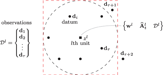
Figure 2. Representation of the lth computing unit and the neighboring data used to approximate the local sensorimotor model. The black and red dashed depict the Gaussian and its square approximation.

3.2. Initial Learning Stage

We propose an adaptive method to iteratively compute the local transformation matrix from data observations. To this end, consider the following quadratic cost function for the lth unit:

$\begin{array}{l}{Q}^l=\frac{1}{2}{\displaystyle \sum _{k=1}^{\tau }}{h}^{lk}{\left|\right|{\hat{\text{A}}}_t^l{\text{u}}_k-{\delta }_k\left|\right|}^2\\ =\frac{1}{2}{\displaystyle \sum _{k=1}^{\tau }}{h}^{lk}{\left|\right|\text{F}({\text{u}}_k){\hat{\text{a}}}_t^l-{\delta }_k\left|\right|}^2& (9)\end{array}$

for $\text{F}({\text{u}}_k)\in {ℝ}^{m\times mn}$ as a regression-like matrix defined as

$\begin{array}{ll}\text{F}({\text{u}}_k)=\left[\begin{array}{cccc}{\text{u}}_k^{⊺}& 0_n^{⊺}& \cdots & 0_n^{⊺}\\ 0_n^{⊺}& {\text{u}}_k^{⊺}& \cdots & 0_n^{⊺}\\ ⋮& ⋮& \ddots & ⋮\\ 0_n^{⊺}& 0_n^{⊺}& \cdots & {\text{u}}_k^{⊺}\end{array}\right]& (10)\end{array}$

and a vector of adaptive parameters ${\hat{\text{a}}}_t^l\in {ℝ}^{nm}$ constructed as:

$\begin{array}{ll}{\hat{\text{a}}}_t^l={\left[\begin{array}{cccc}{â}_t^{l11}& {â}_t^{l12}& \cdots & {â}_t^{lmn}\end{array}\right]}^{⊺}& (11)\end{array}$

where the scalar ${â}_t^{lij}$ denotes the ith row jth column element of the matrix ${\hat{\text{A}}}_t^l$.

The scalar h^lk represents a Gaussian neighborhood function centered at the lth unit and computed as:

$\begin{array}{ll}{h}^{lk}=exp\left(-\frac{\left|\right|{\text{w}}^l-{\text{x}}_k|{|}^2}{2{\sigma }^2}\right)& (12)\end{array}$

where σ > 0 (representing the standard deviation) is used to control the width of the neighborhood. By using h^lk, the observations' contribution to the cost (9) proportionally decreases with the distance to w^l. The dimension of the neighborhood is defined such that h ≈ 0 is never satisfied for any of its observations x^k. In practice, it is common to approximate the Gaussian shape with a simple “square” region, which presents the highest approximation error around its corners (see e.g., Figure 2 where the sampling point d_τ+1 is within its boundary).

To compute an accurate sensorimotor model, the data points in (8) should be as distinctive as possible (i.e., the motor observations u_t should not be collinear). This requirement can be fairly achieved by covering the uncertain configuration with curved/random motions.

The following gradient descent rule is used for approximating the transformation matrix A_t at the lth unit:

$\begin{array}{l}{\hat{\text{a}}}_{t+1}^l={\hat{\text{a}}}_t^l-\gamma \nabla Q^l({\hat{\text{a}}}_t^l)\\ ={\hat{\text{a}}}_t^l-\gamma {\displaystyle \sum _{k=1}^{\tau }}{h}^{lk}\text{F}{({\text{u}}_k)}^{⊺}\left({\hat{\text{A}}}_t^l{\text{u}}_k-{\delta }_k\right)& (13)\end{array}$

for γ > 0 as a positive learning gain. For ease of implementation, the update rule (13) can be equivalently expressed in scalar form as:

$\begin{array}{ll}{â}_{t+1}^{lij}={â}_t^{lij}-\gamma {\displaystyle \sum _{k=1}^{\tau }}{h}^{lk}{u}_k^j\left\{\left({\displaystyle \sum _{r=1}^n}{â}_t^{lir}{u}_k^r\right)-{\delta }_k^i\right\}& (14)\end{array}$

where $u_k^j$ and ${\delta }_k^i$ denote the jth and ith components of the vectors u_k and δ_k, respectively.

Remark 2. There are other estimation methods in the literature that also make use of Gaussian functions, e.g., radial basis functions (RBF) (Li and Cheah, 2014) to name an instance. However, RBF (in its standard formulation) use configuration-dependent Gaussians to modulate a set of weights (which provide non-linear approximation capabilities), whereas in our case, the Gaussians are used but within the weights' adaptation law to proportionally scale the contribution of the collected sensory-motor data (our method provides a linear approximation within the neighborhood). Our Gaussian weighted approach most closely resembles the one used in self organizing maps (SOM) (Kohonen, 2013) to combine surrounding data observations.

3.3. Lyapunov Stability

In this section, we analyse the stability properties of the proposed update rule by using discrete-time Lyapunov theory (Bof et al., 2018). To this end, let us first assume that the transformation matrix satisfies:

$\begin{array}{ll}\text{A}({\text{w}}^l)=\partial f/\partial \text{x}({\text{w}}^l)\approx \text{A}({\text{x}}_j)& (15)\end{array}$

for any configuration x_j around the neighborhood defined by ${{D}}^l$ (this situation implies that A(·) is constant around the vicinity of w^l). Therefore, we can locally express around w^l the sensor changes as:

$\begin{array}{ll}{\delta }_k=\text{F}({\text{u}}_k){\text{a}}^l& (16)\end{array}$

where a^l = [a^l11, a^l12, …, a^lmn]^⊺ ∈ ℝ^mn denotes the vector of constant parameters, for a^lij as the ith row jth column of the unknown matrix A(w^l). To simplify notation, we shall denote F_k = F(u_k).

Proposition 1. For a number mn of linearly independent vectors u_k, the adaptive update rule (13) asymptotically minimizes the magnitude of the parameter estimation error $\left|\right|{\hat{\text{a}}}_t^l-{\text{a}}^l\left|\right|$.

Proof: Consider the following quadratic (energy-like) function:

$\begin{array}{ll}{V}_t^l={\left|\right|{\hat{\text{a}}}_t^l-{\text{a}}^l\left|\right|}^2& (17)\end{array}$

Computing the forward difference of $V_t^l$ yields:

$\begin{array}{l}{V}_{t+1}^l-V_t^l={\left|\right|{\hat{\text{a}}}_{t+1}^l-{\text{a}}^l\left|\right|}^2-{\left|\right|{\hat{\text{a}}}_t^l-{\text{a}}^l\left|\right|}^2\\ ={\left|\right|\left[\text{I}-\gamma {\displaystyle \sum _{k=1}^{\tau }}{h}^{lk}{\text{F}}_k^{⊺}{\text{F}}_k\right]\left({\hat{\text{a}}}_t^l-{\text{a}}^l\right)\left|\right|}^2\\ -{\left|\right|{\hat{\text{a}}}_t^l-{\text{a}}^l\left|\right|}^2=-{\left({\hat{\text{a}}}_t^l-{\text{a}}^l\right)}^{⊺}\Omega \left({\hat{\text{a}}}_t^l-{\text{a}}^l\right)\end{array}$

for a symmetric matrix Ω ∈ ℝ^mn×mn defined as follows:

$\begin{array}{l}\Omega =\text{I}-{\left[\text{I}-\gamma {\displaystyle \sum _{k=1}^{\tau }}{h}^{lk}{\text{F}}_k^{⊺}{\text{F}}_k\right]}^2\\ =2\gamma {\displaystyle \sum _{k=1}^{\tau }}{h}^{lk}{\text{F}}_k^{⊺}{\text{F}}_k-{\gamma }^2{\left[{\displaystyle \sum _{k=1}^{\tau }}{h}^{lk}{\text{F}}_k^{⊺}{\text{F}}_k\right]}^2\\ =\gamma {\Phi }^{⊺}{\displaystyle \underset{\text{C}}{{\displaystyle \underbrace{(2\text{H}-\gamma \text{H}\Phi {\Phi }^{⊺}\text{H})}}}}\Phi & (18)\end{array}$

with $\text{H}=diag(h^{l1}{\text{I}}_{\tau },\dots ,h^{l\tau }{\text{I}}_{\tau })\in {ℝ}^{m\tau \times m\tau }$ as a positive-definite diagonal matrix, ${\text{I}}_{\tau }\in {ℝ}^{\tau \times \tau }$ as an identity matrix and Φ ∈ ℝ^mτ×mn constructed with τ matrices F_k as follows:

$\begin{array}{ll}\Phi ={\left[\begin{array}{cccc}{\text{F}}_1^{⊺}& {\text{F}}_2^{⊺}& \cdots & {\text{F}}_{\tau }^{⊺}\end{array}\right]}^{⊺}& (19)\end{array}$

To prove the asymptotic stability of (13), we must first prove the positive-definiteness of the dissipation-like matrix Ω (van der Schaft, 2000). To this end, note that since the “tall” observations' matrix Φ is exactly known and H is diagonal and positive (hence full-rank), we can always find a gain γ > 0 to guarantee that the symmetric matrix

$\begin{array}{ll}\text{C}=2\text{H}-\gamma \text{H}\Phi {\Phi }^{⊺}\text{H}>0,& (20)\end{array}$

is also positive-definite, and therefore, full-rank. Next, let us re-arrange mn linearly independent row vectors from Φ as follows:

$\begin{array}{ll}\left[\begin{array}{cccc}{\text{u}}_1^{⊺}& 0_n^{⊺}& \cdots & 0_n^{⊺}\\ {\text{u}}_2^{⊺}& 0_n^{⊺}& \cdots & 0_n^{⊺}\\ ⋮& ⋮& ⋮& ⋮\\ {\text{u}}_n^{⊺}& 0_n^{⊺}& \cdots & 0_n^{⊺}\\ 0_n^{⊺}& {\text{u}}_{n+1}^{⊺}& \cdots & 0_n^{⊺}\\ 0_n^{⊺}& {\text{u}}_{n+2}^{⊺}& \cdots & 0_n^{⊺}\\ ⋮& ⋮& \ddots & ⋮\\ 0_n^{⊺}& 0_n^{⊺}& \cdots & {\text{u}}_{mn-1}^{⊺}\\ 0_n^{⊺}& 0_n^{⊺}& \cdots & {\text{u}}_{mn}^{⊺}\end{array}\right]& (21)\end{array}$

which shows that Φ has a full column rank, hence, the matrix Ω = γΦ^⊺CΦ > 0 is positive-definite. This condition implies that $V_{t+1}^l-V_t^l<0$ for any $\left|\right|{\hat{\text{a}}}_t^l-{\text{a}}^l\left|\right|\ne 0$. Asymptotic stability of the parameter's estimation error directly follows by invoking Lyapunov's direct method (Bof et al., 2018).

Remark 3. There are two conditions that need to be satisfied to ensure the algorithm's stability. The first condition is related to the magnitude of the learning gain γ. Large gain values may lead to numerical instabilities, which is a common situation in discrete-time adaptive systems. To find a “small enough” gain γ > 0, we can conduct the simple 1D search shown in Algorithm 1. An eigenvalue test on C can be used to verify (20). The second condition is related to the linear independence (i.e., the non-collinearity) of the motor actions u_t. Such independent vectors are needed for providing a sufficient number of constraints to the estimation algorithm (this condition can be easily satisfied by performing random babbling-like motions).

ALGORITHM 1

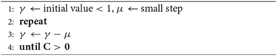
Algorithm 1. Compute a suitable γ.

3.4. Localized Adaptation

Once the cost function (9) has been minimized, the computed transformation matrix ${\hat{\text{A}}}_t$ locally approximates the robot's sensorimotor model around the lth unit. Note that the stability of the total N units is analogous the analysis shown in the previous section; A global analysis is out of the scope of this work.

The associated local training data (8) must then be released from memory to allow for new relations to be learnt—if needed. However, for the case where changes in the sensorimotor conditions occur, the model may contain inaccuracies in some or all computing units, and thus, its transformation matrices cannot be used for controlling the robot's motion. To cope with this issue, we need to first quantitatively assess such errors. For that, the following weighted distortion metric is introduced:

$\begin{array}{ll}{U}_t={\text{e}}_t^{⊺}\text{B}{\text{e}}_t& (22)\end{array}$

where B > 0 denotes a positive-definite diagonal weight matrix to homogenize different scales in the approximation error ${\text{e}}_t={\hat{\text{A}}}^s{\text{u}}_t-{\delta }_t\in {ℝ}^m$. The scalar index s is found by solving the search problem:

$\begin{array}{ll}s={\displaystyle \underset{j}{arg min}}||{\text{w}}^j-{\text{x}}_t||& (23)\end{array}$

To enable adaptation of problematic units, we evaluate the magnitude of the metric U_t, and if found to be larger than an arbitrary threshold U_t > |ε|, new motion and sensor data must be collected around the sth computing unit to construct the revised structure ${{D}}^s$ by using a push approach:

$\begin{array}{ll}{\text{d}}_1\leftarrow \left[\begin{array}{ccc}{\text{x}}_t& {\text{u}}_t& {\delta }_t\end{array}\right]& (24)\end{array}$

that updates the topmost observation and discards the oldest (bottom) data, so as to keep a constant number τ of data points. The transformation matrices are then computed with the new data.

3.5. Motion Controller

The update rule (13) computes an adaptive transformation matrix ${\hat{\text{A}}}_t^l$ for each of the N units in the system. To provide a smooth transition between different units, let us introduce the matrix ${\text{L}}_t\in {ℝ}^{m\times n}$ which is updated as follows³:

$\begin{array}{ll}{\text{L}}_{t+1}={\text{L}}_t-\eta ({\text{L}}_t-{\hat{\text{A}}}_t^s)& (25)\end{array}$

where η > 0 is a tuning gain. The above matrix represents a filtered version of ${\hat{\text{A}}}_t^s$, where s denotes the index of the active unit, as defined in (23). With this approach, the transformation matrix smoothly changes between adjacent neighborhoods, while providing stable values in the vicinity of the active unit; It can be seen as a continuous interpolation between adjacent neighborhoods.

The motor command with adaptive model is implemented as follows:

$\begin{array}{ll}{\text{u}}_t=-\lambda {\text{L}}_t^{\#}sat({\text{y}}_t-{\text{y}}^{*})& (26)\end{array}$

The stability of this kinematic control method can be analyzed with its resulting closed-loop first-order system (a practice also commonly adopted with visual servoing controllers; Chaumette and Hutchinson, 2006). To this end, we use a small displacement approach (motivated by the local target provided by the saturation function), where we introduce the increment vector $\text{i}=-sat({\text{y}}_t-{\text{y}}^{*})$ and define the local reference position $\overline{\text{y}}={\text{y}}_t+\text{i}\in {ℝ}^m$. Let us consider the case when the N units have minimized the cost functions (9). Note that the asymptotic minimization of $\left|\right|{\hat{\text{a}}}_t^l-{\text{a}}^l\left|\right|$ implies that ${\hat{\text{A}}}_t^s$ inherits the rank properties of A_t, hence, the existence of the pseudo-inverse in (26) is guaranteed; A regularization term (see e.g., Tikhonov et al., 2013) can further be used to robustify the computation of ${\text{L}}_t^{\#}$.

Proposition 2. For n ≥ m (i.e., more/equal motor actions than feedback features), the “stiff” kinematic control input (26) provides the local feedback error ${\text{y}}_t-\overline{\text{y}}$ with asymptotic stability.

Proof: Substitution of the controller (26) into the difference model (3) yields the closed-loop system:

$\begin{array}{l}{\text{y}}_{t+1}={\text{y}}_t-\lambda sat({\text{y}}_t-{\text{y}}^{*})={\text{y}}_t+\lambda \text{i}\pm \lambda {\text{y}}_t\\ ={\text{y}}_t-\lambda {\text{y}}_t+\lambda \overline{\text{y}}={\text{y}}_t-\lambda ({\text{y}}_t-\overline{\text{y}})& (27)\end{array}$

Adding $\pm \overline{\text{y}}$ to (27) and after some algebraic operation, we obtain:

$\begin{array}{ll}({\text{y}}_{t+1}-\overline{\text{y}})=(1-\lambda )({\text{y}}_t-\overline{\text{y}})& (28)\end{array}$

which for a gain satisfying 0 < λ < 1, it implies local asymptotic stability of the small displacement error $({\text{y}}_t-\overline{\text{y}})$ (Kuo, 1992).

Remark 4. Note that the above stability analysis assumes that robot's trajectories are not perturbed by external forces and that the estimated interaction matrix locally satisfies ${\text{A}}_t{\text{L}}_t^{\#}{\text{A}}_t\approx {\text{A}}_t$ around the active neighborhood.

4. Case of Study

In this section, we validate the performance of the proposed method with numerical simulations and experiments. A vision-based manipulation task with a deformable cable is used as our case of study (Bretl and McCarthy, 2014): It consists in the robot actively deforming the object into a desired shape by using visual feedback of the cable's contour (see e.g., Zhu et al., 2018). Soft object manipulation tasks are challenging—and relevant to the fundamental problem addressed here—since the sensorimotor models of deformable objects are typically unknown or subject to large uncertainties (Sanchez et al., 2018). Therefore, the transformation matrix relating the shape feature functional and the robot motions is difficult to compute. The proposed algorithm will be used to adaptively approximate the unknown model. Figure 3 conceptually depicts the setup of this sensorimotor control problem.

FIGURE 3

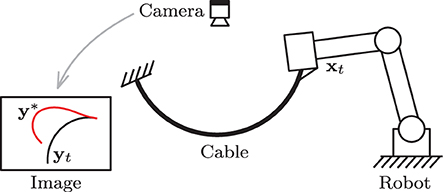
Figure 3. Representation of the cable manipulation case of study, where a vision sensor continuously measures the cable's feedback shape y_t, which must be actively deformed toward y*.

4.1. Simulation Setup

For this study, we consider a planar robot arm that rigidly grasps one end of an elastic cable, whose other end is static; We assume that the total motion of this composed cable-robot system remains on the plane. A monocular vision sensor observes the manipulated cable and measures its 2D contour in real-time. The dynamic behavior of the elastic cable is simulated as in Wakamatsu and Hirai (2004) by using the minimum energy principle (Hamill, 2014), whose solution is computed using the CasADi framework (Andersson et al., 2019). The cable is assumed to have negligible plastic behavior. All numerical simulation algorithms are implemented in MATLAB. The cable simulation code is publicly available at https://github.com/Jihong-Zhu/cableModelling2D.

Let the long vector ${\text{s}}_t\in {ℝ}^{2\alpha }$ represents the 2D profile of the cable, which is simulated using a resolution of α = 100 data points. To perform the task, we must compute a vector of feedback features y_t that characterizes the object's configuration. For that, we use the approach described in Digumarti et al. (2019) and Navarro-Alarcon and Liu (2018) that approximates s_t with truncated Fourier series (in our case, we used four harmonics), and then constructs y_t with the respective Fourier coefficients (Collewet and Chaumette, 2000). The use of these coefficients as feedback signals enable us to obtain a compact representation of the object's configuration, however, it complicates the analytical derivation of the matrix A_t.

4.2. Approximation of the Matrix A_t

To construct the data structure (8), we collect τ = 40 data observations d_t at random locations around the manipulation workspace. Next, we define local neighborhoods centered at the configuration points w¹ = [0.3, 0.5], w² = [0.5, 0.5], w³ = [0.5, 0.3], and w⁴ = [0.5, 0.5]. These neighborhoods are defined with a standard deviation of σ = 1.3. With the collected observations, l = 1, …, 4 matrices ${\hat{\text{A}}}_t^l$ are computed using the update rule (14).

Figure 4 depicts the measured shape (black solid line) of the cable at the four points w^l and the shape that is approximated (red dashed line) with the feedback feature vector y_t (i.e the Fourier coefficients). It shows that four harmonics provide sufficient accuracy for representing the object's configuration. To evaluate the accuracy of the computed discrete configuration space and its associated matrices ${\hat{\text{A}}}_t^l$, we conduct the following test: The robot is commanded to move the cable along a circular trajectory that passes through the four points w^l. The following energy function is computed throughout this trajectory:

$\begin{array}{ll}G={\left|\right|{\delta }_t-{\hat{\text{A}}}_t^l{\text{u}}_t\left|\right|}^2& (29)\end{array}$

which quantifies the accuracy of the local differential mapping (3). The index l switches (based on the solution of 23) as the robot enters a different neighborhood.

FIGURE 4

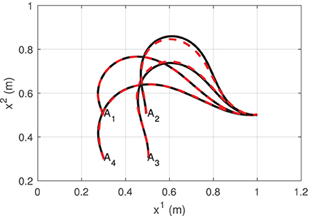
Figure 4. Various configurations of the visually measured cable profile (black solid line) and its approximation with Fourier series (red dashed line).

Figure 5 depicts the profile of the function G along the trajectory. We can see that this error function increases as the robot approaches the neighborhood's boundary. The “switch” label indicates the time instant when ${\text{A}}_t^l$ switches to different (more accurate) matrix, an action that decreases the magnitude of G. This result confirms that the proposed adaptive algorithm provides local directional information on how the motor actions transform into sensor changes.

FIGURE 5

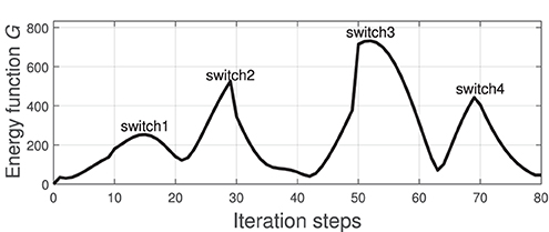
Figure 5. Profile of the function G that is computed along the circular trajectory passing through the points in Figure 4; The “switch” label indicates the instant when ${\hat{\text{A}}}_t^l$ switches to different one.

4.3. Sensor-Guided Motion

In this section, we make use of the approximated sensorimotor model to guide the motion of a robotic system based on feedback features. To this end, various cable shapes are defined as target configurations y^* (to provide physically feasible targets, these shapes are collected from previous sensor observations). The target configurations are then given to the motion controller (26) to automatically perform the task. The controller implemented with saturation bounds of |sat(·)| ≤ 2 and a feedback gain λ = 0.1.

Figure 6 depicts the progression of the cable shapes obtained during these numerical simulations. The initial y₀ and the intermediate configurations are represented with solid black curves, whereas the final shape y^* is represented with red dashed curves. To assess the accuracy of the controller, the following cost function is computed throughout the shaping motions:

$\begin{array}{ll}E=\left|\right|{\text{y}}_t-{\text{y}}^{*}|{|}^2& (30)\end{array}$

For these four shaping actions, Figure 7 depicts the time evolution of the function E. This figure clearly shows that the feedback error is asymptotically minimized.

FIGURE 6

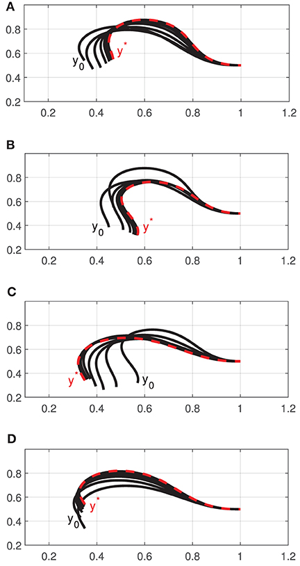
Figure 6. Initial and final configurations of four different shape control simulations (A–D), using a single robot manipulator.

FIGURE 7

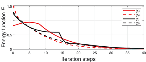
Figure 7. Minimization process of the energy function E.

Now, consider the setup depicted in Figure 8, which has two 3-DOF robots jointly manipulating the deformable cable. For this more complex scenario, the total configuration vector x_t must be constructed with the 3-DOF pose (position and orientation) vectors of both robot manipulators as ${\text{x}}_t={{[}^L{\text{x}}_t^{⊺},{}^R{\text{x}}_t^{⊺}]}^{⊺}$ ∈ ℝ⁶. Training of the sensorimotor model is done similarly as with the single-robot case described above; The same feedback gains and controller parameters are also used in this test.

FIGURE 8

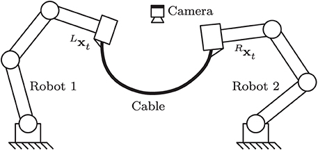
Figure 8. Representation of a two-robot setup where both systems must jointly shape the cable into a desired form.

Figure 9 depicts the initial shape y₀ and intermediate configurations (black solid curves), as well as the respective final shape y^* (red dashed curve) of the cable. Note that as more input DOF can be controlled by the robotic system, the object can be actively deformed into more complex configurations (cf. the achieved S-shape curve with the profiles in Figure 6). The result demonstrates that the approximated sensorimotor model provides sufficient directional information to the controller to properly “steer” the feature vector y_t toward the target y^*.

FIGURE 9

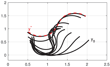
Figure 9. Initial and final configurations of the shape control simulation with two robots.

We now compare the performance of our method (using the same manipulation task shown in Figures 8, 9) with two state-of-the-art approaches commonly used for guiding robots with unknown sensorimotor models. To this end, we consider the classical Broyden update rule (Broyden, 1965) and the recursive least-squares (RLS) (Hosoda and Asada, 1994). These two methods are used for estimating the matrix A that is needed to compute the control input (6). To compare their performance, the cost function E is evaluated throughout their respective trajectories; The same feedback gain λ = 0.1 is used for these three methods. Figure 10 depicts the time evolution of E computed with the three methods. This result demonstrates that the performance of our method is comparable to the other two classical approaches.

FIGURE 10

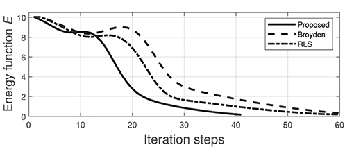
Figure 10. Minimization process of the energy function E.

4.4. Experiments

To validate the proposed theory, we developed an experimental platform composed of a three degrees-of-freedom serial robotic manipulator (DOBOT Magician), a Linux-based motion control system (Ubuntu 16.04), and a USB Webcam (Logitech C270); Image processing is performed by using the OpenCV libraries (Bradski, 2000). A sampling time of dt ≈ 0.04 s is used in our Linux-based control system. In this setup, the robot rigidly grasps an elastic piece of pneumatic air tubing, whose other end is attached to the ground. The 3-DOF mechanism has a double parallelogram structure that enables to control the gripper's x-y-z position while keeping a constant orientation. For this experimental study, we only control 2-DOF of the robot such it manipulates the tubing with plane motions. Figure 11 depicts the setup.

FIGURE 11

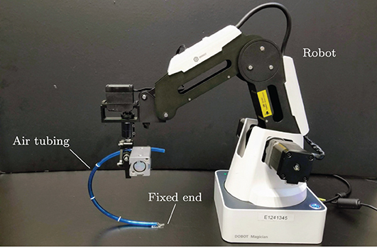
Figure 11. The experimental robotic setup.

We conduct similar vision-guided experiments with the platform as the ones described in the previous section. For these tasks, the elastic tubing must be automatically positioned into a desired contour. The configuration dependant feedback for this task is computed with the observed contour of the object by using two harmonic terms (Navarro-Alarcon and Liu, 2018). The sensorimotor model is similarly approximated around four configuration points (as in Figure 4), by performing random motions and collecting sensor data.

Figure 12 depicts snapshots of the conducted experiments, where we can see the initial and final configurations of the system. The red curves represent the (static) target configuration y^*. For these two targets, Figure 13 depicts the respective time evolution profiles of the energy function E, where we can clearly see that the feedback error is asymptotically minimized. The control inputs u_t used during the experiments are depicted in Figures 14, 15. These motion commands are computed from raw vision measurements and a saturation threshold of ±1 is applied to its values. This results demonstrate that the approximated model can be used to locally guide motions of the robot with sensor feedback.

FIGURE 12

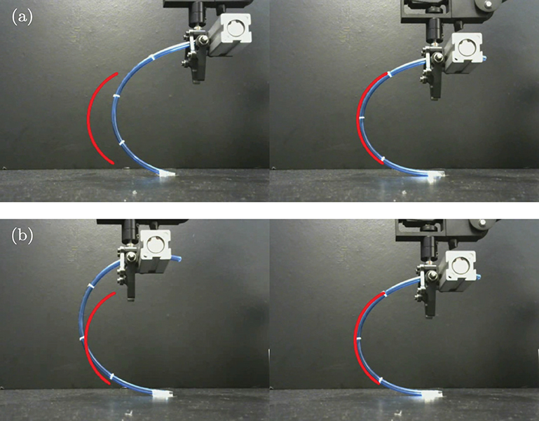
Figure 12. Snapshots of the initial (left) and final (right) configurations for two shape control experiments (a) and (b), where the red curve represents the target shape.

FIGURE 13

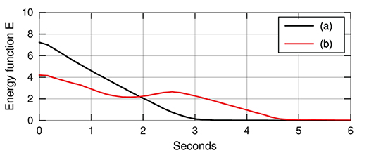
Figure 13. Asymptotic minimization of the error functional E obtained with the experiments shown in Figure 12.

FIGURE 14

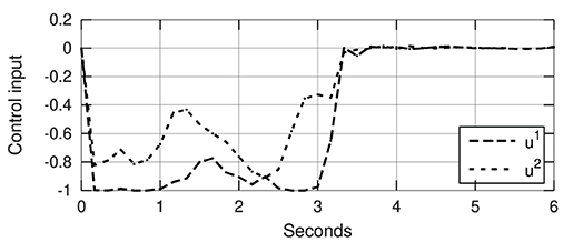
Figure 14. Control input (with normalized units of pixel/s) of the experiment shown in Figure 12a.

FIGURE 15

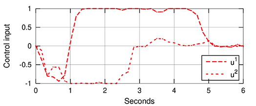
Figure 15. Control input (with normalized units of pixel/s) of the experiment shown in Figure 12b.

5. Conclusion

In this paper, we describe a method to estimate sensorimotor relations of robotic systems. For that, we present a novel adaptive rule that computes local sensorimotor relations in real-time; The stability of this algorithm is rigorously analyzed and its convergence conditions are derived. A motion controller to coordinate sensor measurements and robot motions is proposed. Simulation and experimental results with a cable manipulation case of study are reported to validate the theory.

The main idea behind the proposed method is to divide the robot's configuration workspace into discrete nodes, and then, locally approximate at each node the mappings between robot motions and sensor changes. This approach resembles the estimation of piecewise linear systems, except that in our case, the computed model represents a differential Jacobian-like relation. The key to guarantee the stability of the algorithm lies in collecting sufficient linear independent motor actions (such condition can be achieved by performing random babbling motions).

The main limitation of the proposed algorithm is the local nature of its model, which can be improved by increasing the density of the distributed computing units. Another issue is related to the scalability of its discretized configuration space. Note that for 3D spaces, the method can fairly well approximate the sensorimotor model, yet for multiple DOF (e.g., more than 6) the data is difficult to manage and visualize.

As future work, we would like to implement our adaptive method with other sensing modalities and mechanical configurations, e.g., with an eye-in-hand visual servoing (where the camera orientation is arbitrary) and with variable morphology manipulators (where the link's length and joint's configuration are not known).

Data Availability Statement

The original contributions presented in the study are included in the article/supplementary material, further inquiries can be directed to the corresponding author/s.

Author Contributions

DN-A conceived the algorithm and drafted the manuscript. JQ and JZ performed the numerical simulation results. AC analyzed the theory and revised the paper. All authors contributed to the article and approved the submitted version.

Funding

This research work was supported in part by the Research Grants Council (RGC) of Hong Kong under grant number 14203917, in part by PROCORE-France/Hong Kong Joint Research Scheme sponsored by the RGC and the Consulate General of France in Hong Kong under grant F-PolyU503/18, in part by the Chinese National Engineering Research Centre for Steel Construction (Hong Kong Branch) at PolyU under grant BBV8, in part by the Key-Area Research and Development Program of Guangdong Province 2020 under project 76 and in part by The Hong Kong Polytechnic University under grant G-YBYT.

Conflict of Interest

The authors declare that the research was conducted in the absence of any commercial or financial relationships that could be construed as a potential conflict of interest.

Footnotes

1. ^This can be easily obtained with constant kinematic transformations.

2. ^This difference equation represents the discrete-time model of the robot's differential sensor kinematics.

3. ^For simplicity, we initialize L₀ = 0_n×n with a zero matrix.

References

Alambeigi, F., Wang, Z., Hegeman, R., Liu, Y., and Armand, M. (2018). A robust data-driven approach for online learning and manipulation of unmodeled 3-d heterogeneous compliant objects. IEEE Robot. Autom. Lett. 3, 4140–4147. doi: 10.1109/LRA.2018.2863376

CrossRef Full Text | Google Scholar

Andersson, J. A. E., Gillis, J., Horn, G., Rawlings, J. B., and Diehl, M. (2019). CasADi-A software framework for nonlinear optimization and optimal control. Math. Prog. Comp. 11, 1–36. doi: 10.1007/s12532-018-0139-4

CrossRef Full Text | Google Scholar

Bof, N., Carli, R., and Schenato, L. (2018). Lyapunov theory for discrete time systems. CoRR abs/1809.05289. Available online at: https://arxiv.org/abs/1809.05289

Bouyarmane, K., Chappellet, K., Vaillant, J., and Kheddar, A. (2019). Quadratic programming for multirobot and task-space force control. IEEE Trans. Robot. 35, 64–77. doi: 10.1109/TRO.2018.2876782

CrossRef Full Text | Google Scholar

Bradski, G. (2000). The OpenCV library. Dr. Dobb's J. Softw. Tools 25, 122–125.

Bretl, T., and McCarthy, Z. (2014). Quasi-static manipulation of a Kirchhoff elastic rod based on a geometric analysis of equilibrium configurations. Int. J. Robot. Res. 33, 48–68. doi: 10.1177/0278364912473169

CrossRef Full Text | Google Scholar

Broyden, C. G. (1965). A class of methods for solving nonlinear simultaneous equations. Math. Comp. 19, 577–593. doi: 10.1090/S0025-5718-1965-0198670-6

CrossRef Full Text | Google Scholar

Chang, H., Wang, S., and Sun, P. (2018). Omniwheel touchdown characteristics and adaptive saturated control for a human support robot. IEEE Access 6, 51174–51186. doi: 10.1109/ACCESS.2018.2869836

CrossRef Full Text | Google Scholar

Chaumette, F., and Hutchinson, S. (2006). Visual servo control. Part I: Basic approaches. IEEE Robot. Autom. Mag. 13, 82–90. doi: 10.1109/MRA.2006.250573

CrossRef Full Text | Google Scholar

Cheah, C. C., Hirano, M., Kawamura, S., and Arimoto, S. (2003). Approximate Jacobian control for robots with uncertain kinematics and dynamics. IEEE Trans. Robot. Autom. 19, 692–702. doi: 10.1109/TRA.2003.814517

CrossRef Full Text | Google Scholar

Cherubini, A., and Chaumette, F. (2013). Visual navigation of a mobile robot with laser-based collision avoidance. Int. J. Robot. Res. 32, 189–205. doi: 10.1177/0278364912460413

CrossRef Full Text | Google Scholar

Cherubini, A., Passama, R., Fraisse, P., and Crosnier, A. (2015). A unified multimodal control framework for human-robot interaction. Robot. Auton. Syst. 70, 106–115. doi: 10.1016/j.robot.2015.03.002

CrossRef Full Text | Google Scholar

Collewet, C., and Chaumette, F. (2000). “A contour approach for image-based control on objects with complex shape,” in Proceedings of IEEE/RSJ International Conference on Intelligent Robots and Systems, Vol. 1 (Takamatsu), 751–756. doi: 10.1109/IROS.2000.894694

CrossRef Full Text | Google Scholar

Defoort, M., and Murakami, T. (2009). Sliding-mode control scheme for an intelligent bicycle. IEEE Trans. Indus. Electron. 56, 3357–3368. doi: 10.1109/TIE.2009.2017096

CrossRef Full Text | Google Scholar

Digumarti, K. M., Trimmer, B., Conn, A. T., and Rossiter, J. (2019). Quantifying dynamic shapes in soft morphologies. Soft Robot. 1, 1–12. doi: 10.1089/soro.2018.0105

PubMed Abstract | CrossRef Full Text | Google Scholar

Escobar-Juarez, E., Schillaci, G., Hermosillo-Valadez, J., and Lara-Guzman, B. (2016). A self-organized internal models architecture for coding sensory–motor schemes. Front. Robot. AI 3:22. doi: 10.3389/frobt.2016.00022

CrossRef Full Text | Google Scholar

Falkenhahn, V., Mahl, T., Hildebrandt, A., Neumann, R., and Sawodny, O. (2015). Dynamic modeling of bellows-actuated continuum robots using the euler-lagrange formalism. IEEE Trans. Robot. 31, 1483–1496. doi: 10.1109/TRO.2015.2496826

CrossRef Full Text | Google Scholar

Hamill, P. (2014). A Student's Guide to Lagrangians and Hamiltonians. New York, NY: Cambridge University Press.

Google Scholar

Haykin, S. (2009). Neural Networks and Learning Machines. Ontario: Prentice Hall.

PubMed Abstract | Google Scholar

Hosoda, K., and Asada, M. (1994). “Versatile visual servoing without knowledge of true Jacobian,” in Proceedings of IEEE/RSJ International Conference on Intelligent Robots and Systems, Vol. 1 (Munich), 186–193. doi: 10.1109/IROS.1994.407392

CrossRef Full Text | Google Scholar

Hu, Z., Han, T., Sun, P., Pan, J., and Manocha, D. (2019). 3-D deformable object manipulation using deep neural networks. IEEE Robot. Autom. Lett. 4, 4255–4261. doi: 10.1109/LRA.2019.2930476

CrossRef Full Text | Google Scholar

Huang, J., and Lin, C.-F. (1994). On a robust nonlinear servomechanism problem. IEEE Trans. Autom. Control 39, 1510–1513. doi: 10.1109/9.299646

CrossRef Full Text | Google Scholar

Hutchinson, S., Hager, G., and Corke, P. (1996). A tutorial on visual servo control. IEEE Trans. Robot. Autom. 12, 651–670. doi: 10.1109/70.538972

CrossRef Full Text | Google Scholar

Jagersand, M., Fuentes, O., and Nelson, R. (1997). “Experimental evaluation of uncalibrated visual servoing for precision manipulation,” in Proceedings of IEEE International Conference on Robotics and Automation, Vol. 4 (Albuquerque, NM), 2874–2880. doi: 10.1109/ROBOT.1997.606723

CrossRef Full Text | Google Scholar

Kohler, I. (1962). Experiments with goggles. Sci. Am. 206, 62–73. doi: 10.1038/scientificamerican0562-62

PubMed Abstract | CrossRef Full Text | Google Scholar

Kohonen, T. (2001). Self-Organizing Maps. Berlin; Heidelberg: Springer. doi: 10.1007/978-3-642-56927-2

CrossRef Full Text | Google Scholar

Kohonen, T. (2013). Essentials of the self-organizing map. Neural Netw. 37, 52–65. doi: 10.1016/j.neunet.2012.09.018

PubMed Abstract | CrossRef Full Text | Google Scholar

Kuo, B. (1992). Digital Control Systems. Electrical Engineering. New York, NY: Oxford University Press.

Google Scholar

Li, X., and Cheah, C. C. (2014). Adaptive neural network control of robot based on a unified objective bound. IEEE Trans. Control Syst. Technol. 22, 1032–1043. doi: 10.1109/TCST.2013.2293498

CrossRef Full Text | Google Scholar

Liu, Y.-H., Wang, H., Chen, W., and Zhou, D. (2013). Adaptive visual servoing using common image features with unknown geometric parameters. Automatica 49, 2453–2460. doi: 10.1016/j.automatica.2013.04.018

CrossRef Full Text | Google Scholar

Lyu, S., and Cheah, C. C. (2018). “Vision based neural network control of robot manipulators with unknown sensory Jacobian matrix,” in IEEE/ASME International Conference on Advanced Intelligent Mechatronics (Auckland), 1222–1227. doi: 10.1109/AIM.2018.8452467

CrossRef Full Text | Google Scholar

Magassouba, A., Bertin, N., and Chaumette, F. (2016). “Audio-based robot control from interchannel level difference and absolute sound energy,” in Proceedings of IEEE International Conference on Intelligent Robots and Systems (Daejeon), 1992–1999. doi: 10.1109/IROS.2016.7759314

CrossRef Full Text | Google Scholar

Nakamura, Y. (1991). Advanced Robotics: Redundancy and Optimization. Boston, MA: Addison-Wesley Longman.

Google Scholar

Navarro-Alarcon, D., Cherubini, A., and Li, X. (2019). “On model adaptation for sensorimotor control of robots,” in Chinese Control Conference (Guangzhou), 2548–2552. doi: 10.23919/ChiCC.2019.8865825

CrossRef Full Text | Google Scholar

Navarro-Alarcon, D., and Liu, Y.-H. (2018). Fourier-based shape servoing: a new feedback method to actively deform soft objects into desired 2D image shapes. IEEE Trans. Robot. 34, 272–279. doi: 10.1109/TRO.2017.2765333

CrossRef Full Text | Google Scholar

Navarro-Alarcon, D., Liu, Y.-H., Romero, J. G., and Li, P. (2014). Energy shaping methods for asymptotic force regulation of compliant mechanical systems. IEEE Trans. Control Syst. Technol. 22, 2376–2383. doi: 10.1109/TCST.2014.2309659

CrossRef Full Text | Google Scholar

Navarro-Alarcon, D., Yip, H., Wang, Z., Liu, Y.-H., Zhong, F., Zhang, T., et al. (2016). Automatic 3D manipulation of soft objects by robotic arms with adaptive deformation model. IEEE Trans. Robot. 32, 429–441. doi: 10.1109/TRO.2016.2533639

CrossRef Full Text | Google Scholar

Navarro-Alarcon, D., Yip, H. M., Wang, Z., Liu, Y.-H., Lin, W., and Li, P. (2015). “Adaptive image-based positioning of RCM mechanisms using angle and distance features,” in IEEE/RSJ International Conference on Intelligent Robots and Systems (Hamburg), 5403–5409. doi: 10.1109/IROS.2015.7354141

CrossRef Full Text | Google Scholar

Nof, S. (1999). Handbook of Industrial Robotics. New Jersey, NJ: John Wiley & Sons. doi: 10.1002/9780470172506

CrossRef Full Text | Google Scholar

Pierris, G., and Dahl, T. S. (2017). Learning robot control using a hierarchical som-based encoding. IEEE Trans. Cogn. Dev. Syst. 9, 30–43. doi: 10.1109/TCDS.2017.2657744

CrossRef Full Text | Google Scholar

Saegusa, R., Metta, G., Sandini, G., and Sakka, S. (2009). “Active motor babbling for sensorimotor learning,” in International Conference on Robotics and Biomimetics (Bangkok), 794–799. doi: 10.1109/ROBIO.2009.4913101

CrossRef Full Text | Google Scholar

Sanchez, J., Corrales, J.-A., Bouzgarrou, B.-C., and Mezouar, Y. (2018). Robotic manipulation and sensing of deformable objects in domestic and industrial applications: a survey. Int. J. Robot. Res. 37, 688–716. doi: 10.1177/0278364918779698

CrossRef Full Text | Google Scholar

Sang, Q., and Tao, G. (2012). Adaptive control of piecewise linear systems: the state tracking case. IEEE Trans. Autom. Control 57, 522–528. doi: 10.1109/TAC.2011.2164738

CrossRef Full Text | Google Scholar

Saponaro, P., Sorensen, S., Kolagunda, A., and Kambhamettu, C. (2015). “Material classification with thermal imagery,” in IEEE Conference on Computer Vision and Pattern Recognition (Boston, MA), 4649–4656. doi: 10.1109/CVPR.2015.7299096

CrossRef Full Text | Google Scholar

Siciliano, B. (1990). Kinematic control of redundant robot manipulators: a tutorial. J. Intell. Robot. Syst. 3, 201–212. doi: 10.1007/BF00126069

CrossRef Full Text | Google Scholar

Sigaud, O., Salaün, C., and Padois, V. (2011). On-line regression algorithms for learning mechanical models of robots: a survey. Rob. Auton. Syst. 59, 1115–1129. doi: 10.1016/j.robot.2011.07.006

CrossRef Full Text | Google Scholar

Tikhonov, A., Goncharsky, A., Stepanov, V., and Yagola, A. (2013). Numerical Methods for the Solution of Ill-Posed Problems. Mathematics and Its Applications. Dordrecht: Springer Netherlands.

Google Scholar

Tirindelli, M., Victorova, M., Esteban, J., Kim, S. T., Navarro-Alarcon, D., Zheng, Y. P., et al. (2020). Force-ultrasound fusion: Bringing spine robotic-us to the next “level”. IEEE Robot. Autom. Lett. 5, 5661–5668. doi: 10.1109/LRA.2020.3009069

CrossRef Full Text | Google Scholar

van der Schaft, A. (2000). L₂-Gain and Passivity Techniques in Nonlinear Control. London: Springer. doi: 10.1007/978-1-4471-0507-7

CrossRef Full Text | Google Scholar

Von Hofsten, C. (1982). Eye-hand coordination in the newborn. Dev. Psychol. 18:450. doi: 10.1037/0012-1649.18.3.450

CrossRef Full Text | Google Scholar

Wakamatsu, H., and Hirai, S. (2004). Static modeling of linear object deformation based on differential geometry. Int. J. Robot. Res. 23, 293–311. doi: 10.1177/0278364904041882

CrossRef Full Text | Google Scholar

Wang, H., Liu, Y.-H., and Zhou, D. (2008). Adaptive visual servoing using point and line features with an uncalibrated eye-in-hand camera. IEEE Trans. Robot. 24, 843–857. doi: 10.1109/TRO.2008.2001356

CrossRef Full Text | Google Scholar

Wang, Z., Yip, H. M., Navarro-Alarcon, D., Li, P., Liu, Y., Sun, D., et al. (2016). Design of a novel compliant safe robot joint with multiple working states. IEEE/ASME Trans. Mechatron. 21, 1193–1198. doi: 10.1109/TMECH.2015.2500602

CrossRef Full Text | Google Scholar

Wei, G.-Q., Arbter, K., and Hirzinger, G. (1986). Active self-calibration of robotic eyes and hand-eye relationships with model identification. IEEE Trans. Robot. Autom. 14, 158–166. doi: 10.1109/70.660864

CrossRef Full Text | Google Scholar

Whitney, D. (1969). Resolved motion rate control of manipulators and human prostheses. IEEE Trans. Man-Mach. Syst. 10, 47–53. doi: 10.1109/TMMS.1969.299896

CrossRef Full Text | Google Scholar

Yip, H. M., Navarro-Alarcon, D., and Liu, Y. (2017). “An image-based uterus positioning interface using adaline networks for robot-assisted hysterectomy,” in IEEE International Conference on Real-time Computing and Robotics (Okinawa), 182–187. doi: 10.1109/RCAR.2017.8311857

CrossRef Full Text | Google Scholar

Yu, C., Zhou, L., Qian, H., and Xu, Y. (2018). “Posture correction of quadruped robot for adaptive slope walking,” in IEEE International Conference on Robotics and Biomimetics (Malaysia), 1220–1225. doi: 10.1109/ROBIO.2018.8665093

CrossRef Full Text | Google Scholar

Zahra, O., and Navarro-Alarcon, D. (2019). “A self-organizing network with varying density structure for characterizing sensorimotor transformations in robotic systems,” in Towards Autonomous Robotic Systems, eds K. Althoefer, J. Konstantinova, K. Zhang (London: Springer), 167–178. doi: 10.1007/978-3-030-25332-5_15

CrossRef Full Text | Google Scholar

Zhu, J., Navarro, B., Fraisse, P., Crosnier, A., and Cherubini, A. (2018). “Dual-arm robotic manipulation of flexible cables,” in IEEE/RSJ Int. Conf. on Robots and Intelligent Systems (Madrid), 479–484. doi: 10.1109/IROS.2018.8593780

CrossRef Full Text | Google Scholar