Multi-Modal Image Fusion Based on Matrix Product State of Tensor

1. Introduction

The purpose of image fusion is to synthesize multiple images of the same scene into a fusion image containing part or all information of each source image (Zhang, 2004). The fused image contains more information than each source image, thus, it is more suitable for machine processing and human visual perception. Image fusion has a wide range of applications in many fields, such as computer vision, remote sensing, medical imaging, and video surveillance (Goshtasby and Nikolov, 2007). The same type of sensors acquire information in a similar way, so the single-modal image fusion cannot provide information of the same scene from different aspects. On the contrary, multi-modal image fusion (Ma et al., 2019) realizes the complementarity of different features of the same scene through fusing the images collected by different types of sensors and generates an informative image for subsequent processing. As typical multi-modal images, infrared and visible images, CT and MRI images can provide distinctive features and complementary information, that is, infrared images can capture thermal radiation signal and visible images can capture reflected light signal; CT is mainly used for signal acquisition of sclerous tissue (e.g., bones), and MRI is mainly used for signal acquisition of soft tissue. Therefore, multi-modal image fusion has a wide range of applications in engineering practice.

To realize image fusion, many scholars have proposed a large number of fusion algorithms in recent years. In general, the fusion methods can be divided into two categories: the spatial-domain methods and the transform-domain methods. The typical methods in the first category include the weighted average method and principal component analysis (PCA) method (Yu et al., 2011) and so on. They fuse the gray values of image pixels directly. Although the direct operation on the pixels has low complexity, the fusion process is less robust to noise, and the results cannot meet the needs of the application in most cases. To overcome this shortcoming, a fusion method based on transform is proposed (Burt and Adelson, 1983; Haribabu and Bindu, 2017; Li et al., 2019). In general, the transform-based methods obtain the transformed coefficients of an image using a certain set of base functions, then fuse these coefficients through certain fusion rules, and finally obtain the final fused image through the corresponding inverse transform. For example, Burt and Adelson (1983) formed a laplacian pyramid (LP) by desampling and filtering source images, and then designed different fusion strategies at each layer. Finally, the fused image is obtained by applying the inverse transform on the fusion coefficients. Haribabu and Bindu (2017) first decomposed the source images by using discrete wavelet transform (DWT) and fused the coefficients with predefined fusion rules, and then obtained the final image by applying the inverse discrete wavelet transform on fused coefficients. Because the transform-based method employs the average weighted fusion rules for the low-frequency components which carry the most energy of the image, there will be something wrong with the contrast loss of the final fused image.

In addition to traditional spatial-domain and transform-domain methods, sparse representation (SR) has been extensively used in image fusion in recent years (Yang and Li, 2010; Jiang and Wang, 2014; Liu et al., 2016; Zhang and Levine, 2016). The SR method assumes that the signal to be processed satisfies y ∈ Rⁿ, then y = Dx, where D ∈ R^n×m(n << m) is an overcomplete dictionary, and n is the dimensions of the signal and m is the number of atoms in the dictionary D which is formed by a set of image subblocks, x is the sparse coefficients vector. The fused image is reconstructed by means of fusing the sparse coefficients. Although the SR-based method has achieved many results in the field of image fusion, some detailed information will be lost in the reconstructed image (e.g., the edges and textures tend to be smoothed), which limits the ability of the SR to express images (Yang and Li, 2010). To solve this problem, some scholars proposed some improved algorithms (Jiang and Wang, 2014; Liu et al., 2016). For instance, Jiang and Wang (2014) used morphological component analysis (MCA) to represent the source images more effectively. The MCA method first applied SR to separate the source images into two parts: cartoon and texture, then different fusion rules were designed to fuse these two parts respectively. Finally, a fused image with rich information was obtained, and more characteristic features of the source images were preserved.

As an extension of the vector and matrix, the tensor (Kolda and Bader, 2009) plays an important role in the high-dimensional data processing. In the field of computer science and technology, a tensor is a multi-dimensional array. It can be extended to some common data types, for example, a zero-order tensor can be defined as a constant, the tensor of order 1 is defined as a vector, the tensor of order 2 is defined as a matrix, the tensor of order 3 and the tensor of order N (N ≥ 3) is called high-order tensor. In essence, tensor decomposition is a high-order generalization of matrix decomposition, which is mainly applied to dimensionality reduction, sparse data filling, and implicit relationship mining. The information processing method based on tensor is more suitable for the processing of high-dimensional data and the extraction of feature information than vector and matrix, therefore, some relevant applications have been emerged in recent years (Bengua et al., 2015, 2017a,b; Zhang et al., 2016). In view of the excellent performance of tensors in representing high-dimensional data and feature extraction, a tensor-based high-order singular value decomposition method (HOSVD) (Liang et al., 2012) was applied to image fusion and achieved good results. In this method, the source image is initialized into a tensor which is subsequently decomposed into several sub-tensors by using a sliding window technique. Then, the HOSVD is applied on each sub-tensors to extract the corresponding features which are fused by employing certain fusion rules.

Since HOSVD is an approximate decomposition method, it will lead to the loss of information in the process of image fusion. At the same time, the calculation process is large and a stable closed-form solution cannot be obtained. To avoid loss of detailed information, a novel method based on matrix product state (MPS) is proposed to fuse the multi-modal images. Compared with HOSVD, MPS achieves the improvement of HOSVD and achieves the purpose of acquisition image information accurately. Moreover, being different from SR who linearly represents images by using atoms in an overcomplete dictionary, MPS decomposes image tensor into MPS. The main difference is that SR is approximate decomposition, while MPS is accurate decomposition. Therefore, in terms of signal reconstruction, MPS has better performance in signal expression. The main contributions of the article are outlined as follows: (i) Considering that image fusion depends more on local information of the source images and dividing the image into blocks can get more details of each pixel, the two source images are first divided into several sub-image blocks, and then the corresponding sub-image blocks are initialized into sub-tensors; (ii) We perform the MPS on each sub-tensor separately to obtain the corresponding core matrixes. The core matrixes are fused using the fusion rule based on the sigmoid function which incorporates the conventional choose-max strategy and the weighted average strategy. This fusion strategy can preserve the features of the multi-modal source images and reduce the loss of contrast to the greatest extent; (iii) Due to the application of MPS, the computational complexity of image fusion based on tensor is reduced dramatically. Hence, MPS decomposition is realized by computing a series of sub-tensors with maximum order 3. Moreover, a stable closed-form solution can also be obtained in the proposed algorithm.

The rest of the article is organized as follows. Section 2 introduces the theory of matrix product decomposition. In section 3, the algorithm principle and the fusion steps are detailly discussed. Subsequently, the results of the experiments are presented in section 4. Finally, some conclusions are drawn in section 5.

2. MPS for Tensor

2.1. Tensor

Tensor is a generalization of the vector. A vector is a kind of tensor with order 1. For simplicity and accuracy of the following expressions, first, we introduce some notations about tensors. The tensor of order 0 is a constant, represented by lowercase letter x; the tensor of order 1 is a vector represented by a bold lowercase letter x; the tensor of order 2 is a matrix represented by a bold capital letter X; the tensor of order 3 is a tensor represented by bold capital letters in italics X. In this way, a tensor of order N and the size of each dimension are I₁ × I₂ × ⋯ × I_N can be expressed as $X\in R^{I_1\times I_2\times \cdots \times I_N}$, where I_i corresponds to the length of the i-th dimension. In general, we use x_i1 ⋯ x_iN to represent the (i₁, ⋯ , i_N)-th element of X.

2.2. MPS for Tensor

The MPS decomposition (Perez-Garcia et al., 2006; Schollwock, 2011; Schuch et al., 2011; Sanz et al., 2016) aims to decompose an N-dimensional tensor X into the corresponding left-right orthogonal factor matrix and a core matrix. First, all the dimensions of an N-dimensional tensor X are rearranged, which lets the dimension K corresponding to the number of images to be fused, for example, if the number of source images is equal to 2, then K = 2. Additionally, the tensor X satisfies $X\in R^{I_1\times \cdots \times I_{n-1}\times K\times I_n\times \cdots \times I_N}$, I₁ ≥ ⋯ ≥ I_n−1, I_n ≤ ⋯ ≤ I_N, then the elements in the tensor X can be expressed in the form of MPS, and the schematic diagram of MPS form of X is shown in Figure 1:

$\begin{array}{ll}{x}_{i_1\cdots k\cdots i_N}=x_{i_1\cdots i_n\cdots i_N}^{(k)}\approx {\text{L}}_{i_1}^{(1)}\cdots {\text{L}}_{i_{n-1}}^{(n-1)}{\text{C}}_k^{(n)}{\text{R}}_{i_n}^{(n+1)}\cdots {\text{R}}_{i_N}^{(N+1)}.& (1)\end{array}$

${\mathbf{\text{L}}}_{i_j}^{(j)}$ and ${\mathbf{\text{R}}}_{i_{(j-1)}}^{(j)}$ mentioned in the above formula are called left-right orthogonal factor matrix with size δ_j−1 × δ_j, where δ₀ = δ_N+1 = 1, and they are all orthogonal:

$\begin{array}{ll}{\displaystyle \sum _{i_j=1}^{I_j}}(L_{i_j}^{(j)}{)}^T{\text{L}}_{i_j}^{(j)}=\text{I},(j=1,\cdots ,n-1)& (2)\end{array}$

and

$\begin{array}{ll}{\displaystyle \sum _{i_{j-1}=1}^{I_{j-1}}}{\text{R}}_{i_{j-1}}^{(j)}(R_{i_{j-1}}^{(j)}{)}^T=\text{I},(j=n+1,\cdots ,N+1),& (3)\end{array}$

where I is an identity matrix, ${\mathbf{\text{C}}}_k^n$ is called core matrix.

FIGURE 1

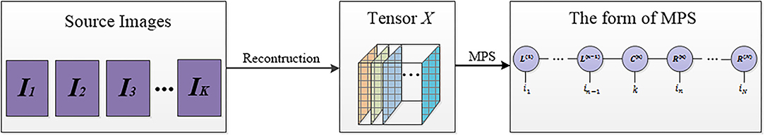
Figure 1. The matrix product state (MPS) form of X.

A tensor X can be decomposed into the form of (1) through two series of SVD decomposition. The process includes a left-to-right sweep and a right-to-left sweep. We summarize it in Algorithm 1.

ALGORITHM 1

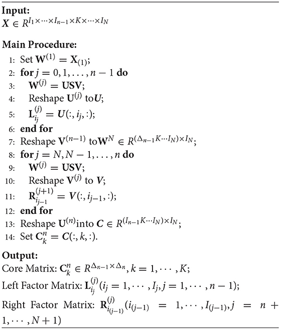
Algorithm 1. Feature Extraction based on MPS

3. Image Fusion Based on MPS

In this section, the whole process of image fusion will be described. The source images which have been reconstructed into tensors are decomposed into a series of sub-tensors by using the sliding window technology. The graphical representation of the sliding window technology is shown in Figure 2. Then MPS is applied to the decomposed sub-tensors to obtain the core matrixes, and the sigmoid function is used for the fusion of each pair of core matrixes to obtain the fused core matrixes.

FIGURE 2

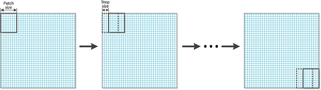
Figure 2. The graphical representation of the sliding window technology.

The specific theoretical concepts of decomposition and fusion are described in sections 3.1, 3.2, respectively, and the overall process of image fusion proposed in this article is described in section 3.3.

3.1. Tensor Decomposition by MPS

For the two source images A and B with sizes of M × N, we use them to construct a tensor X with dimension M × N × 2. Taking into account the importance of local information of the source image, a sliding window technology is used to decompose it into several sub-tensors F with dimension $\overline{M}\times \overline{N}\times 2$, and the sliding step p used should satisfy $p\le min\left\{\overline{M},\overline{N}\right\}$; the sub-tensor F is obtained by the Algorithm 2, as follows. In Algorithm 2, the fix((M − patch size)/stepsize) represents the nearest integer to (M − patch size)/stepsize and fix((N − patch size)/stepsize) represents the nearest integer to (N − patch size)/stepsize. Then, MPS is applied to each of the sub-tensors.

ALGORITHM 2

Algorithm 2. The Sub-tensor obtained by Sliding Window Technology

3.2. Design of Fusion Rule

We introduce the sigmoid function as the fusion rule of the characteristic coefficients, the fusion coefficient of each core matrix can be defined as follows:

$\begin{array}{ll}{e}_i(l)={\displaystyle \sum _{m=1}^{\bar{M}}}{\displaystyle \sum _{n=1}^{\bar{N}}}|{\text{C}}_i(m,n,l)|l=1,2& (4)\end{array}$

where the subscript i indicates the number of each sub-image, and l is the label of the corresponding source image.

For e_i(l) obtained in the previous section, the fusion rule is selected by comparing the values of e_i(1) and e_i(2). When e_i(1) is much less or much more than e_i(2), we use the Max rule, and when the relationship between e_i(1) and e_i(2) satisfy the other relation, we use weighted fusion to fuse the corresponding coefficient matrix and then get the final fusion coefficient matrix. The function is as follows:

$\begin{array}{l}{D}_i=\frac{1}{1+exp(-kln(\frac{e_i(1)}{e_i(2)}))}\\ \times {\text{C}}_i(:,:,1)+\frac{exp(-kln(\frac{e_i(1)}{e_i(2)}))}{1+exp(-kln(\frac{e_i(1)}{e_i(2)}))}\times {\text{C}}_i(:,:,2)& (5)\end{array}$

where k is the shrinkage factor of the mentioned sigmoid function. After D_i is obtained, each of the fused sub-image blocks F_i can be reconstructed by the inverse operations of MPS. Then the sub-image blocks F_i is used to obtain the final fused image G.

To make the process of decomposition and fusion more concrete, the first group of the experiment images is used as an example to make a flowchart as shown in Figure 3:

FIGURE 3

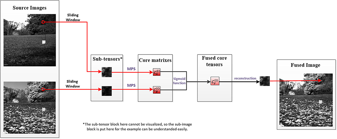
Figure 3. An example for visualizing the process of decomposition and fusion.

3.3. The Process of Image Fusion Based on MPS

The process of image fusion based on MPS can be divided into the seven steps as follows

1. Input two source images;

2. Reconstructed the two source images into a third-order tensor, and the sub-tensors are extracted by sliding window technology;

3. Matrix product state decomposition is used on sub-tensors to obtain left and right factor matrixes and core matrixes;

4. Compare the vectors representing source image 1 and source image 2 in the core matrixes obtained in step 3, and obtain the fused matrixes by corresponding their quantitative relations to different situations of the sigmoid function, and then construct it as sub-tensors;

5. Multiply the fused sub-tensors by left and right factor tensors to obtain sub-images;

6. Sub-images addition;

7. Output fused image.

The specific flowchart is shown in Figure 4.

FIGURE 4

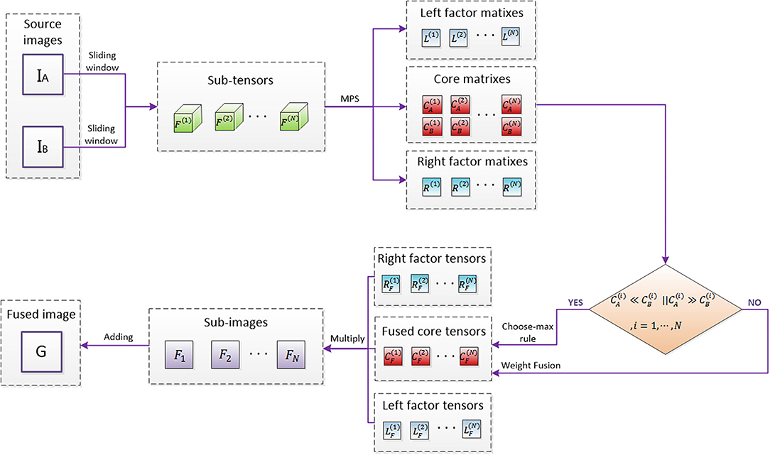
Figure 4. Fusion flowchart based on MPS.

4. Experiments

4.1. Objective Evaluation Metrics

1. Standard deviation (SD)

SD is defined as follows:

$\begin{array}{ll}SD=\sqrt{\frac{1}{H\times W}{\displaystyle \sum _{x=1}^H}{\displaystyle \sum _{y=1}^W}{(F(x,y)-\mu )}^2},& (6)\end{array}$

where μ is the average value of the fused image, H and W are the length and width of the image, respectively. SD is mainly used to measure the contrast of the fused image.

2. Mutual information (MI)

Mutual information is defined as follows:

$\begin{array}{ll}MI={\displaystyle \sum _{x=1}^L}{\displaystyle \sum _{y=1}^L}{h}_{R,F}(i,j)lo{g}_2\frac{h_{R,F}(i,j)}{h_R(i)+h_F(j)},& (7)\end{array}$

where h_R,F(i, j) is the normalized joint distribution gray histogram between the source image R and the fused image F, h_R(i) and h_F(j) are the normalized marginal distribution histogram of the two source images, respectively, L is the number of gray levels.

3. Structural similarity (SSIM)

Structural similarity is defined as follows:

$\begin{array}{ll}SSIM(x,y)=(\frac{2{\mu }_x{\mu }_y+c_1}{{\mu }_x^2+{\mu }_y^2+1}{)}^{\alpha }(\frac{2{\sigma }_x{\sigma }_y+c_1}{{\sigma }_x^2+{\sigma }_y^2+1}{)}^{\beta }(\frac{{\sigma }_{xy}+c_3}{{\sigma }_x{\sigma }_y+c_3}{)}^{\gamma },& (8)\end{array}$

where μ_x and μ_y are the average value of x and y. The middle term represents the similarity of contrast, σ_x and σ_y is the SD of x and y. The right term characterizes the structural similarity, and σ_xy is the covariance of x and y. The c₁, c₂, and c₃ are three constants, and the parameters α, β, and γ, respectively, adjust the contribution of the three terms. SSIM can calculate the similarity between the fused image and the source image. Its value which is between 0 and 1 is closer to 1, the more similar the two images are. The average value of the fused image and the two source images A and B is taken as the final evaluation metric, namely

$\begin{array}{ll}SSIM=\frac{1}{2}(SSI{M}_A+SSI{M}_B).& (9)\end{array}$

4. Gradient based fusion metric (Q_G)

Q_G is defined as follows:

$\begin{array}{ll}{Q}_G=\frac{{\displaystyle {\sum }_{x=1}^H}{\displaystyle {\sum }_{y=1}^W}(Q_{AF}(x,y)w_A(x,y)+Q_{BF}(x,y)w_B(x,y))}{{\displaystyle {\sum }_{x=1}^H}{\displaystyle {\sum }_{y=1}^W}(w_A(x,y)+w_B(x,y))},& (10)\end{array}$

where Q_AF(x, y) = Q_AFg(x, y)Q_AFα(x, y), at each pixel (x, y),Q_AFg(x, y) and Q_AFα(x, y) denote the edge strength and orientation preservation values. Q_BF(x, y) is defined as the same as Q_AF(x, y). The weighting factors w_A(x, y) and w_B(x, y) indicate the significance of Q_AF(x, y) and Q_BF(x, y). Q_G is an important fusion image quality evaluation method computing the amount of gradient information that is injected into the fused image from the source image.

5. Phase congruency based fusion metric (Q_P)

The Q_P is defined as follows:

$\begin{array}{ll}{Q}_P={(P_p)}^{\alpha }{(P_M)}^{\beta }{(P_m)}^{\gamma },& (11)\end{array}$

where p, M, and m refer to phase congruency, maximum, and minimum moments. The parameters α, β, and γ are set to 1 in this article. For more detailed information on parameters, please refer to the article Hong (2000). Q_P measures the extent that the salient features in the source image are preserved.

4.2. Study of Patch Size and Step Size

Considering the sliding window technology is used, we will first study the respective influence of the size of the sub-image block and the step size of the sliding window on the performance of the fusion image experimentally. In the following statement we use patch size and step size to call the two factors briefly. To obtain the optimal patch size and step size, we will use a pair of infrared and visible images as source images, as shown in Figures 5A,B. In the experiment of patch size, the patch size is set to 2 × 2, 4 × 4, 6 × 6, 8 × 8, 10 × 10, 12 × 12, 14 × 14, 16 × 16, 18 × 18, and 20 × 20 with the step size fixed to 1 and shrinkage factor fixed to 200. In the experiment of step size, the step size is set to 1, 2, 4, 6, 8, and 10 with the patch size fixed to 16 × 16 and the shrinkage factor fixed to 200. The experimental results based on the objective evaluation metrics are shown in Tables 1, 2. The output fused images are shown in Figures 5, 6.

FIGURE 5

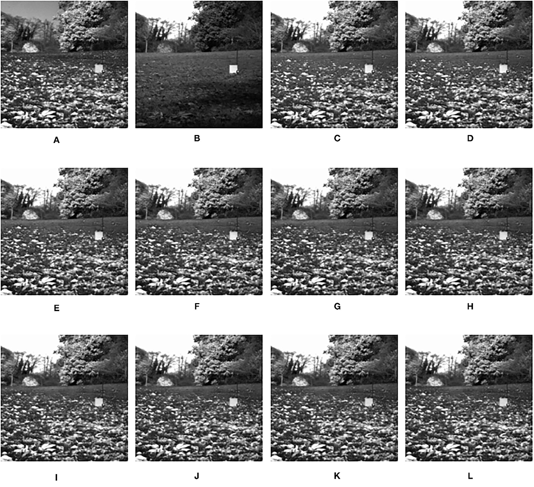
Figure 5. The output fused images in patch size experiment. (A) original image (infrared image); (B) original image (visible image); (C) patch of size 2 × 2; (D) patch of size 4 × 4; (E) patch of size 6 × 6; (F) patch of size 8 × 8; (G) patch of size 10 × 10; (H) patch of size 12 × 12; (I) patch of size 14 × 14; (J) patch of size 16 × 16; (K) patch of size 18 × 18; (L) patch of size 20 × 20.

TABLE 1

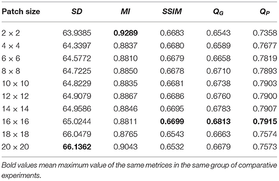
Table 1. The influence of patch size.

TABLE 2

Table 2. The influence of step size.

FIGURE 6

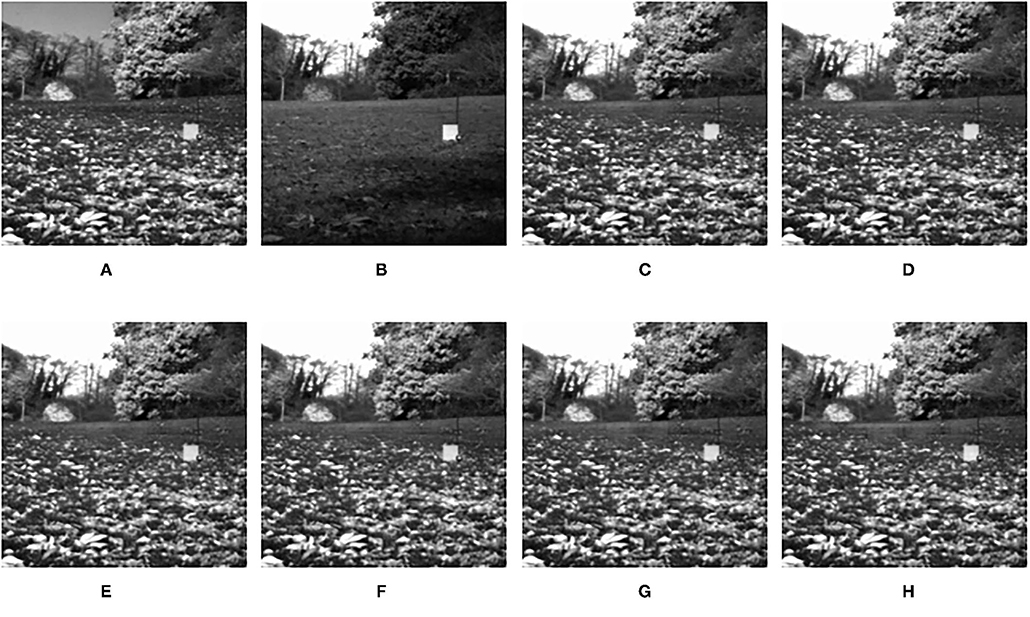
Figure 6. The output fused images in step size experiment. (A) original image (infrared image); (B) original image (visible image); (C) step size = 1; (D) step size = 2; (E) step size = 4; (F) step size = 6; (G) step size = 8; (H) step size = 10.

It can be seen clearly from Table 1, in most cases, that the best results can be obtained when the size of the sub-image block is 16 × 16. According to simple analysis, when the sub-image block is too small, the image characteristics cannot be effectively represented. Additionally, it can be seen from Table 2 that when the step size is 1, the best result can be obtained. According to simple analysis, when the step size is too large, local information of the image may be lost or cannot be displayed well. Therefore, the in following experiments, the patch size was set to 16 × 16, and the step size was set to 1.

4.3. Computation Complexity

The computation time of each group of experimental images is recorded when different fusion algorithms are used. Experimental results show that the complexity of the proposed algorithm is lower than other algorithms. The results are shown in Table 3 as follows:

TABLE 3

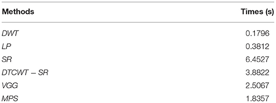
Table 3. Computation times of different algorithms.

All the codes are performed under MATLAB R2014a running on computer equipment with an Intel i7-7700K CPU (4.2 GHz) and 16 GB of RAM. As can be seen from the table, compared with SR and Dual-tree complex wavelet transform-sparse representation (DTCWT-SR), the running of the proposed algorithm is faster. In general, the computational complexity of the proposed algorithm is reduced.

4.4. Experimental Results and Discussion

In this section, the effectiveness of the proposed method is further verified by comparing the experimental results of this algorithm with other fusion methods. The comparison methods used are DWT (Haribabu and Bindu, 2017) and LP (Burt and Adelson, 1983), SR-based methods (Liu et al., 2016), VGG-Net (Hui et al., 2018), and DTCWT-SR (Singh et al., 2012). In addition to the infrared and visible images used in the previous section, CT and MRI medical images are also used for contrast experiments. The performance of each algorithm is evaluated by calculating the evaluation metrics based on the fusion results. In the experiment, all the experimental source image size is 256 × 256, the fixed patch size is 16 × 16, the step size is 1, and the shrinkage factor k is 200. The proposed method and several comparison algorithms are applied to nine pairs of source images. The experimental results are shown in Figures 7–15, respectively. The objective evaluation metrics values of the nine pairs of images are shown in Tables 4, 5.

FIGURE 7

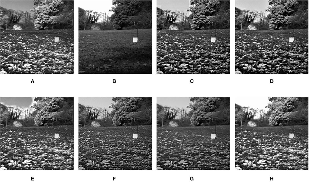
Figure 7. Comparison experimental results of infrared and visible images. (A) original figure (infrared image); (B) original figure (visible image); (C) discrete wavelet transform (DWT); (D) laplacian pyramid (LP); (E) sparse representation (SR); (F) Dual-tree complex wavelet transform-sparse representation (DTCWT-SR); (G) VGG; (H) Matrix product state (MPS).

TABLE 4

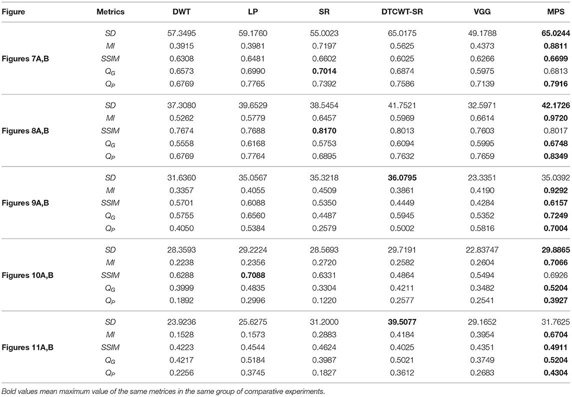
Table 4. Comparison of objective evaluation metrics of infrared and visible images.

TABLE 5

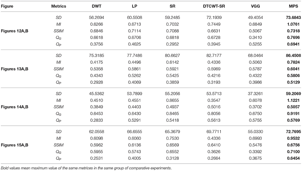
Table 5. Comparison of objective evaluation metrics of CT and MRI images.

It can be seen from the table that in most cases, the algorithm proposed in this article can achieve optimal results, especially for CT and MRI images, the various metrics of the results of MPS are much higher than other methods. For infrared and visible images, the method in this article can also achieve optimal results under more than half of the evaluation metrics. These results show that the proposed method is better than other methods for multi-modal image fusion. This advantage mainly benefits from two aspects: (i) The sliding window method is adopted to divide the image into several sub-images, so the local information of the image can be captured well; (ii) MPS method is an accurate decomposition and reconstruction method, so in the process of image fusion, there will be no loss of information due to the solution.

Further analysis of the experimental results shows that: (i) On the whole, VGG-Net has the worst performance in all cases. Compared with other comparison methods, there is a big gap in various evaluation metrics. This is because the information captured is insufficient in the layer-by-layer feature extraction of the source image, and when the details of the fusion image are weighted by the final weight graph, the contrast of the initial detail part of the fusion image is reduced; (ii) Among the two multi-scale methods used, DWT fusion method performs poorly. This is because the DWT method is based on Haar wavelet to achieve fusion, which can only capture image features in horizontal and vertical directions but cannot capture more basic features of the image; LP method is better than the DWT method because the Laplacian pyramid generates only one band-pass component at each scale, which reduces the possibility of being affected by noise; (iii) The results obtained by SR method are better than other multi-scale methods in most cases but not as good as the proposed method. This is because the signal representation ability of SR is better than that of multi-scale transformation, and errors will occur in the process of signal reconstruction, which is unavoidable for the SR method. The method proposed in this article can effectively avoid this problem by non-destructive tensor reconstruction. In addition, the “max-L1” rule of direct fusion in the spatial domain will lead to spatial inconsistency, which affects the performance of the SR method; (iv) DTCWT-SR is an method that multi-scale method combined with SR method. By comparing the objective evaluation metrics, the fusion performance of the algorithm is better than SR in some aspects, but it is still poor compared with MPS.

In addition to objective evaluation, the performance of the algorithm in this article is also discussed through some visual comparisons of the fused images. In general, the proposed method achieves the best visual effect among all the fusion images.

The fusion results of infrared-visible images are shown in Figures 7–11. It can be seen from the figure that the method proposed in this article has good adaptability, and the fusion images are obtained to retain the information of the infrared and visible images, respectively. In Figure 7, both the multi-scale fusion method and SR show varying degrees of artificial traces at the junction between the trees and the sky in the upper left corner, while DTCWT-SR and VGG-Net resulted in severe contrast loss. In Figure 8, the white squares in infrared picture are dimming in varying degrees in DWT, LP, SR, DTCWT-SR, and VGG-Net methods, and the leaf luster in the visible image is not well-displayed in the VGG-Net method. In Figure 9, DWT and SR show the phenomenon of information loss. LP, DTCWT-SR, and VGG can get relatively complete fusion images, but the brightness is weaker than MPS. The clarity of the billboard in the upper left corner of the fused image is better in the MPS method. In Figure 10, the fused images obtained by DWT and SR show some small black blocks, that is information loss, while the human shape brightness on the right side of the images obtained by LP, DTCWT-SR, and VGG method is low. The reason for these shortcomings is the fusion rules used in the fusion process all have a certain degree of weighting on the source image. Our fusion rules based on the sigmoid function can well avoid these shortcomings, that is, in the image, whose colors are only black and white, the weight of the white part of the image will be much larger than that of the black part, thus, evolving into the Choose-max rule. In Figure 11, compared with the other five comparison methods, it can be seen that the human figure on the right and the branch on the lower right corner of the fusion image obtained by MPS have the highest resolution.

FIGURE 8

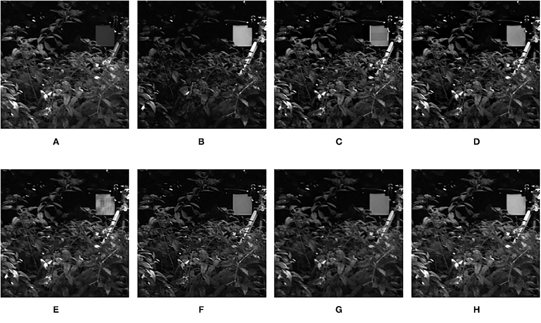
Figure 8. Comparison experimental results of infrared and visible images. (A) original image (infrared image); (B) original image (visible image); (C) DWT; (D) LP; (E) SR; (F) DTCWT-SR; (G) VGG; (H) MPS.

FIGURE 9

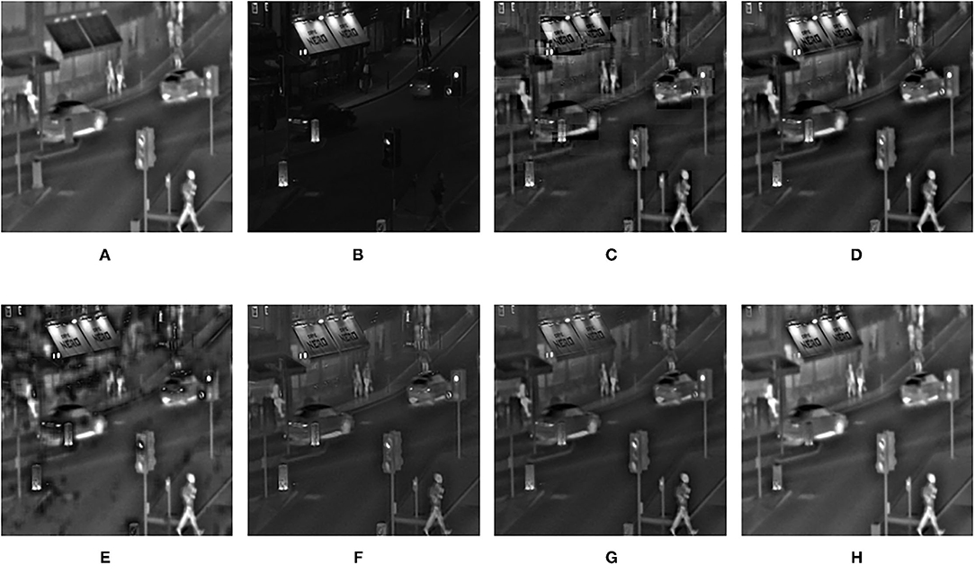
Figure 9. Comparison experimental results of infrared and visible images. (A) original image (infrared image); (B) original image (visible image); (C) DWT; (D) LP; (E) SR; (F) DTCWT-SR; (G) VGG; (H) MPS.

FIGURE 10

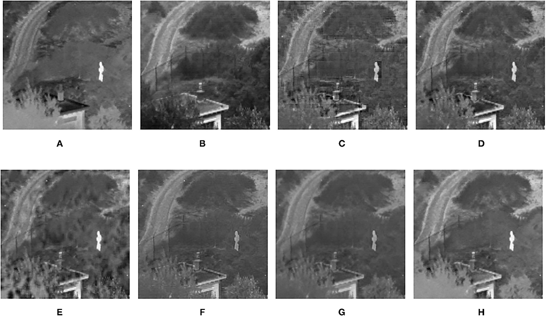
Figure 10. Comparison experimental results of infrared and visible images. (A) original image (infrared image); (B) original image (visible image); (C) DWT; (D) LP; (E) SR; (F) DTCWT-SR; (G) VGG; (H) MPS.

FIGURE 11

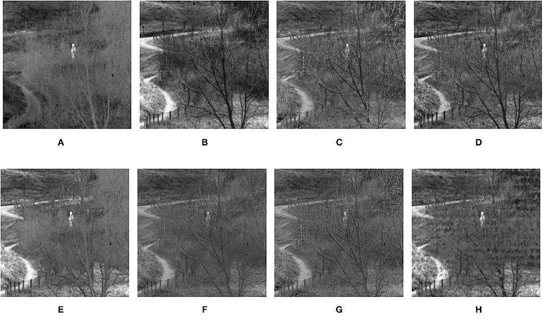
Figure 11. Comparison experimental results of infrared and visible images. (A) original image (infrared image); (B) original image (visible image); (C) DWT; (D) LP; (E) SR; (F) DTCWT-SR; (G) VGG; (H) MPS.

Figures 12–15 are the fusion results of CT and MRI medical images. It can be seen from the experimental results that the DWT method cannot to be applied to the fusion of medical images, and the other four methods can obtain a complete image. In Figure 12, LP, DTCWT-SR, and VGG-Net methods have no loss in details, but the sharpness of the light and dark junction is insufficient, the edge is blurred, and the contrast is lost. However, the bottom of the fused image obtained by the SR method is fractured, indicating that there is information loss. In Figure 13, the spine in the lower right corner and the jaw in the lower left corner of the image obtained by MPS were more clear than the other five methods, the brain vein was also clearer, and the contrast was higher than the other five methods. In Figure 14, the fused images obtained by LP and SR methods were fractured at the lower right corner. Although DTCWT-SR and VGG methods obtained relatively complete fusion images, there is a certain degree of contrast loss. In Figure 15, LP, DTCWT-SR, and VGG-Net methods have some contrast loss, especially in the middle part, at the same time, the image obtained by the SR method presents spatial dislocation at both sides of the eyeball and a certain degree of distortion appears at the position of white connection of the two images. The SR method also has similar shortcomings in this regard, please refer to the lower right corner of the image.

FIGURE 12

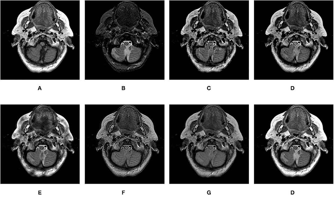
Figure 12. Comparison experimental results of CT and MRI images. (A) original image (CT); (B) original image (MRI); (C) DWT; (D) LP; (E) SR; (F) DTCWT-SR; (G) VGG; (H) MPS.

FIGURE 13

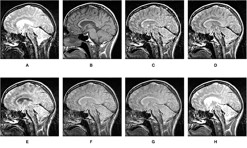
Figure 13. Comparison experimental results of CT and MRI images. (A) original image (CT); (B) original image (MRI); (C) DWT; (D) LP; (E) SR; (F) DTCWT-SR; (G) VGG; (H) MPS.

FIGURE 14

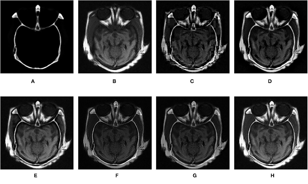
Figure 14. Comparison experimental results of CT and MRI images. (A) original image (CT); (B) original image (MRI); (C) DWT; (D) LP; (E) SR; (F) DTCWT-SR; (G) VGG; (H) MPS.

FIGURE 15

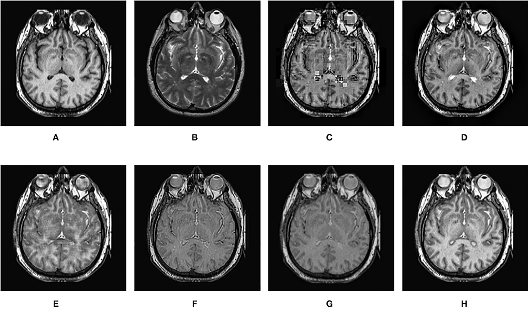
Figure 15. Comparison experimental results of CT and MRI images. (A) original image (CT); (B) original image (MRI); (C) DWT; (D) LP; (E) SR; (F) DTCWT-SR; (G) VGG; (H) MPS.

5. Conclusion

In this article, we propose a method based on MPS for multi-modal image fusion. First, the source images are initialized into a three-dimensional tensor, and then the tensor is decomposed into several sub-tensors by using a sliding window to obtain the corresponding features. The core matrix is fused by the fusion rule based on the sigmoid function, and the fused image is obtained by multiplying the left-right factor matrix. In this article, we use a sliding window to avoid blocking effects, and fully consider the local information of the source images by dividing the source image into a set of sub-images. The experimental results show that the proposed algorithm is feasible and effective for image fusion. Being different from the average fusion rule of the multi-scale method and the “Max-L1” fusion rule of the SR method, the fusion rule based on the sigmoid function used in the article is more effective, but it also makes the fusion process more complicated of the proposed method. Future study will focus on further exploring a more effective fusion rule to improve the fusion results.

Data Availability Statement

The original contributions presented in the study are included in the article/supplementary material, further inquiries can be directed to the corresponding author/s.

Author Contributions

YL designed the algorithm. RW performed experiments and wrote this article. QG, DS, and DZ revised the manuscript. All authors confirmed the submitted version.

Funding

This work was supported by Nature Science Foundation of Anhui (2008085MF183), The Key Science Program of Anhui Education Department (KJ2018A0012), The Research Fund for Doctor of Anhui University (J01003266), and National Natural Science Foundation of China (NSFC)(61402004).

Conflict of Interest

The authors declare that the research was conducted in the absence of any commercial or financial relationships that could be construed as a potential conflict of interest.

Publisher's Note

All claims expressed in this article are solely those of the authors and do not necessarily represent those of their affiliated organizations, or those of the publisher, the editors and the reviewers. Any product that may be evaluated in this article, or claim that may be made by its manufacturer, is not guaranteed or endorsed by the publisher.

Acknowledgments

The authors would like to thank the members in the lab for discussion and valuable suggestions for this study.

References

Bengua, J. A., Phien, H. N., and Tuan, H. D. (2015). “Optimal feature extraction and classification of tensors via matrix product state decomposition,” in 2015 IEEE International Congress on Big Data, 669–672. doi: 10.1109/BigDataCongress.2015.105

CrossRef Full Text | Google Scholar

Bengua, J. A., Phien, H. N., Tuan, H. D., Do, M. N. (2017a). Efficient tensor completion for color image and video recovery: low-rank tensor train. IEEE Trans. Image Process. 26, 2466–2479. doi: 10.1109/TIP.2017.2672439

PubMed Abstract | CrossRef Full Text | Google Scholar

Bengua, J. A., Phien, H. N., Tuan, H. D., and Do, M. N. (2017b). Matrix product state for higher-order tensor compression and classification. IEEE Trans. Signal Process. 65, 4019–4030. doi: 10.1109/TSP.2017.2703882

CrossRef Full Text | Google Scholar

Burt, P., and Adelson, E. (1983). The Laplacian pyramid as a compact image code. IEEE Trans. Commun. 31, 532–540. doi: 10.1109/TCOM.1983.1095851

CrossRef Full Text

Goshtasby, A., and Nikolov, S. (2007). Image fusion: advances in the state of the art. Inform. Fusion 8, 114–118. doi: 10.1016/j.inffus.2006.04.001

CrossRef Full Text | Google Scholar

Haribabu, M., and Bindu, C. H. (2017). “Visibility based multi modal medical image fusion with DWT,” in IEEE Int. Conf. Power, Control, Signals and Instrum. Eng., 1561–1566. doi: 10.1109/ICPCSI.2017.8391973

CrossRef Full Text | Google Scholar

Hong, R. (2000). Objective image fusion performance measure. Military Tech. Courier 56, 181–193. doi: 10.5937/vojtehg0802181B

CrossRef Full Text | Google Scholar

Hui, L., Wu, X. J., and Kittler, J. (2018). “Infrared and visible image fusion using a deep learning framework,” in International Conference on Pattern Recognition 2018.

PubMed Abstract | Google Scholar

Jiang, Y., and Wang, M. (2014). Image fusion with morphological component analysis. Inform. Fusion 18, 107–118. doi: 10.1016/j.inffus.2013.06.001

CrossRef Full Text | Google Scholar

Kolda, T. G., and Bader, B. W. (2009). Tensor decompositions and applications. SIAM Rev. 51, 455–500. doi: 10.1137/07070111X

CrossRef Full Text | Google Scholar

Li, W. S., Du, J., Zhao, Z. M., and Long, J. (2019). Fusion of medical sensors using adaptive cloud model in local Laplacian pyramid domain. IEEE Trans. Biomed. Eng. 66, 1172–1183. doi: 10.1109/TBME.2018.2869432

PubMed Abstract | CrossRef Full Text | Google Scholar

Liang, J. L., He, Y., Liu, D., and Zeng, J. (2012). Image fusion using higher order singular value decomposition. IEEE Trans. Image Process. 21, 2898–2909. doi: 10.1109/TIP.2012.2183140

PubMed Abstract | CrossRef Full Text | Google Scholar

Liu, Y., Chen, X., Ward, R. K., and Wang, Z. J. (2016). Image fusion with convolutional sparse representation. IEEE Signal Process. Lett. 23, 1882–1886. doi: 10.1109/LSP.2016.2618776

PubMed Abstract | CrossRef Full Text | Google Scholar

Ma, J., Ma, Y., and Li, C. (2019). Infrared and visible image fusion methods and applications: a survey. Inform. Fusion 45, 153–178. doi: 10.1016/j.inffus.2018.02.004

CrossRef Full Text | Google Scholar

Perez-Garcia, D., Verstraete, F., Wolf, M. M., and Cirac, J. I. (2006). Matrix product state representations. Physics 7, 401–430. doi: 10.26421/QIC7.5-6-1

CrossRef Full Text | Google Scholar

Sanz, M., Egusquiza, I. L., Candia, R. D., Lamata, L., and Solano, E. (2016). Entanglement classification with matrix product states. Sci. Rep. 6:30188. doi: 10.1038/srep30188

PubMed Abstract | CrossRef Full Text | Google Scholar

Schollwock, U. (2011). The density-matrix renormalization group in the age of matrix product states. Ann. Phys. 326, 96–192. doi: 10.1016/j.aop.2010.09.012

CrossRef Full Text | Google Scholar

Schuch, N., Perez-Garcia, D., and Cirac, I. (2011). Classifying quantum phases using matrix product states and projected entangled pair states. Phys. Rev. 84, 667–673. doi: 10.1103/PhysRevB.84.165139

CrossRef Full Text | Google Scholar

Singh, R., Srivastava, R., Prakash, O., and Khare, A. (2012). “DTCWT based multimodal medical image fusion,” in International conference on Signal, Image and Video processing (ICSIVP-2012), 403–407.

Google Scholar

Yang, B., and Li, S. (2010). Multifocus image fusion and restoration with sparse representation. IEEE Trans. Instrument. Measure. 59, 884–892. doi: 10.1109/TIM.2009.2026612

CrossRef Full Text | Google Scholar

Yu, P., Sun, Q. S., and Xia, D. (2011). Image fusion framework based on decomposition of PCA. Comput. Eng. 37, 210–213.

Google Scholar

Zhang, Q., and Levine, M. D. (2016). Robust multi-focus image fusion using multi-task sparse representation and spatial context. IEEE Trans. Image Process. 25, 2045–2058. doi: 10.1109/TIP.2016.2524212

PubMed Abstract | CrossRef Full Text | Google Scholar

Zhang, X., Wen, G., and Dai, W. (2016). A tensor decomposition-based anomaly detection algorithm for hyperspectral image. IEEE Trans. Geosci. Remote Sens. 54, 5801–5820. doi: 10.1109/TGRS.2016.2572400

CrossRef Full Text | Google Scholar

Zhang, Y. (2004). Understanding image fusion. Photogrammetr. Eng. Remote Sens. 70, 657–661.

Google Scholar