Decision making under uncertainty: a neural model based on partially observable Markov decision processes

Introduction

To survive in a constantly changing and uncertain environment, animals must solve the problem of learning to choose actions based on noisy sensory information and incomplete knowledge of the world. Neurophysiological and psychophysical experiments suggest that the brain relies on probabilistic representations of the world and performs Bayesian inference using these representations to estimate task-relevant quantities (sometimes called “hidden or latent states”) (Knill and Richards, 1996; Rao et al., 2002; Doya et al., 2007). A number of computational models have been proposed to demonstrate how Bayesian inference could be performed in biologically plausible networks of neurons (Rao, 2004, 2005; Yu and Dayan, 2005; Zemel et al., 2005; Ma et al., 2006; Beck et al., 2008; Deneve, 2008). A question that has received less attention is how such probabilistic representations could be utilized to learn actions that maximize expected reward.

In this article, we propose a neural model for action selection and decision making that combines probabilistic representations of the environment with a reinforcement-based learning mechanism to select actions that maximize total expected future reward. The model leverages recent advances in three different fields: (1) neural models of Bayesian inference, (2) the theory of optimal decision making under uncertainty based on partially observable Markov decision processes (POMDPs), and (3) algorithms for temporal difference (TD) learning in reinforcement learning theory.

The new model postulates that decisions are made not based on a unitary estimate of “state” but rather the entire posterior probability distribution over states (the “belief state”) (see also Dayan and Daw, 2008; Frazier and Yu, 2008; Shenoy et al., 2009, 2011). This allows the model to take actions based on the current degree of uncertainty in its estimates. It allows, for example, “information-gathering” actions that can be used to reduce the current uncertainty in an estimate of a task-relevant quantity before committing to a decision. We show how a network of neurons can learn to map belief states to appropriate actions for maximizing expected reward.

We illustrate the proposed model by applying it to the well-known random dots motion discrimination task. We show that after learning, model neurons representing belief state exhibit responses similar to those of LIP neurons in primate cerebral cortex. The appropriate threshold for switching from gathering information to making a decision is learned as part of the reward maximization process through TD learning. After learning, the temporal evolution of reward prediction error (TD error) in the model shares similarities with the responses of midbrain dopaminergic neurons in monkeys performing the random dots task. We also show that the model can learn time-dependent decision making strategies, predicting a collapsing decision threshold for tasks with deadlines.

The model ascribes concrete computational roles to the neocortex and the basal ganglia. Cortical circuits are hypothesized to compute belief states (posterior distributions over states). These belief states are received as inputs by neurons in the striatum in the basal ganglia. Striatal neurons are assumed to represent behaviorally relevant points in belief space which are learned from experience. The model suggests that the striatal/STN-GPe-GPi/SNr network selects the appropriate action for a particular belief state while the striatal-SNc/VTA network computes the value (total expected future reward) for a belief state. The dopaminergic outputs from SNc/VTA are assumed to convey the TD reward prediction error that modulates learning in the striatum-GP/SN networks. Our model thus resembles previous “actor-critic” models of the basal ganglia (Barto, 1995; Houk et al., 1995) but differs in the use of belief states for action selection and value computation.

Model

We first introduce the theory of partially observable Markov decision processes. We then describe the three main components of the model: (1) neural computation of belief states, (2) learning the value of a belief state, and (3) learning the appropriate action for a belief state.

Partially Observable Markov Decision Processes (POMDPs)

Partially observable Markov decision processes (POMDPs) provide a formal probabilistic framework for solving tasks involving action selection and decision making under uncertainty (see Kaelbling et al., 1998 for an introduction). In POMDPs, when an animal executes an action a, the state of the world (or environment) is assumed to change from the current state s’ to a new state s according to the transition probability distribution (or Markov “dynamics”) T(s’, a, s) = P(s|s’, a). A measurement or observation o about the new state s is then generated by the environment according to the probability distribution P(o|s) and the animal receives a real-valued reward r = R(s’, a) (which can be 0, denoting no reward, or some positive or negative value). We focus in this paper on the discrete case: a state is assumed to be one of N discrete values {1, 2, …, N} and an action can be one of K discrete values {1, 2, …, K}. The observations can be discrete or continuous, although in the simulations, we use discrete observations.

The goal of the agent is to maximize the expected sum of future rewards:

where t is a discrete representation of time and takes on the values 0, 1, 2, 3, …, and γ is a “discount factor” between 0 and 1. Equation (1) expresses the general “infinite-horizon” case; a similar equation holds for the finite-horizon case where the expectation is over finite episodes or trials and the discount factor γ can be set to 1. The latter applies, for example, in tasks such as the random dots task studied in the Results section, where trials are of finite duration.

Since the animal does not know the true state of the world, it must choose actions based on the history of observations and actions. This information is succinctly captured by the “belief state,” which is the posterior probability distribution over states at time t, given past observations and actions. When the states are discrete, the belief state is a vector b_t whose size is the number of states. The ith component of b_t is the posterior probability of state i: b_t(i) = P(s_t = i|o_t, a_t−1, o_t−1,…,a₀, o₀).

The belief state can be computed recursively over time from the previous belief state using Bayes rule:

where k is a normalization constant. The simplification of conditional dependencies in the equations above follows from the Markov assumption (current state only depends on previous state and action, and current observation only depends on current state).

The goal then becomes one of maximizing the expected future reward in Eq. (1) by finding an optimal “policy” π which maps a belief state b_t to an appropriate action a_t: π (b_t) = a_t.

Note that in traditional reinforcement learning, states are mapped to actions whereas a POMDP policy maps a belief state (a probability distribution over states) to an action. This adds considerable computational power because it allows the animal to consider the current uncertainty in its state estimates while choosing actions, and if need be, perform “information-gathering” actions to reduce uncertainty.

Methods for solving POMDPs typically rely on estimating the value of a belief state, which, for a fixed policy π, is defined as the expected sum of rewards obtained by starting from the current belief state and executing actions according to π:

This can be rewritten in a recursive form known as Bellman’s equation (Bellman, 1957) for the policy π defined over belief states:

The recursive form is useful because it enables one to derive an online learning rule for value estimation as described below.

Figure 1 summarizes the POMDP model of decision making and the computational elements needed to solve a POMDP problem.

FIGURE 1

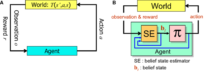
Figure 1. The POMDP model. (A) When the animal executes an action a in the state s’, the environment (“World”) generates a new state s according to the transition probability T(s’,a,s). The animal receives an observation o of the new state according to P(o|s) and a reward r = R(s’,a). (B) In order to solve the POMDP problem, the animal maintains a belief b_t which is a probability distribution over states of the world. This belief is computed iteratively using Bayesian inference by the belief state estimator SE. An action for the current time step is provided by the learned policy π, which maps belief states to actions.

A Neural Model for Learning Actions in POMDPs

We propose here a model for learning POMDP policies that could be implemented in neural circuitry. The model leverages recent advances in POMDP solvers in the field of artificial intelligence as well as ideas from reinforcement learning theory.

Before proceeding to the model, we note that the space of beliefs is continuous (each component of the belief state vector is a probability between 0 and 1) and typically high-dimensional (number of dimensions is one less than the number of states). This makes the problem of finding optimal policies very difficult. In fact, finding exact solutions to general POMDP problems has been proved to be a computationally hard problem (e.g., the finite-horizon case is “PSPACE-hard”; Papadimitriou and Tsitsiklis, 1987). However, one can typically find approximate solutions, many of which work well in practice. Our model is most closely related to a popular class of approximation algorithms known as point-based POMDP solvers (Hauskrecht, 2000; Pineau et al., 2003; Spaan and Vlassis, 2005; Kurniawati et al., 2008). The idea is to discretize the belief space with a finite set of belief points and compute value for these belief points rather than the entire belief space. For learning value, our model relies on the temporal-difference (TD) framework (Sutton and Barto, 1981; Sutton, 1988; Sutton and Barto, 1998) in reinforcement learning theory, a framework that has also proved useful in understanding dopaminergic responses in the primate brain (Schultz et al., 1997).

Neural computation of belief

A prerequisite for a neural POMDP model is being able to compute the belief state b_t in neural circuitry. Several models have been proposed for neural implementation of Bayesian inference (see Rao, 2007 for a review). We focus here on one potential implementation. Recall that the belief state is updated at each time step according to the following equation:

where b_t(i) is the ith component of the belief vector b_t and represents the posterior probability of state i.

Equation (2) combines information from the current observation (P(o_t|s_t)) with feedback from the past time step (b_t−1), suggesting a neural implementation based on a recurrent network, for example, a leaky integrator network:

where v denotes the vector of output firing rates, o denotes the input observation vector, f₁ is a potentially non-linear function describing the feedforward transformation of the input, M is the matrix of recurrent synaptic weights, and g₁ is a dendritic filtering function.

The above differential equation can be rewritten in discrete form as:

where v_t(i) is the ith component of the vector v, f and g are functions derived from f₁ and g₁, and M(i,j) is the synaptic weight value in the ith row and jth column of M.

To make the connection between Eq. (4) and Bayesian inference, note that the belief update Eq. (2) requires a product of two sources of information (current observation and feedback) whereas Eq. (4) involves a sum of observation- and feedback-related terms. This apparent divide can be bridged by performing belief updates in the log domain:

This suggests that Eq. (4) could neurally implement Bayesian inference over time as follows: the log likelihood log P(o_t|s_t = i) is computed by the feedforward term f(o_t) while the feedback conveys the log of the predicted distribution, i.e., logΣ_jT(j, a_t−1,i)b_t−1(j), for the current time step. The latter is computed from the activities v_t−1(j) from the previous time step and the recurrent weights M(i,j), which is defined for each action a. The divisive normalization in Eq. (2) reduces in the equation above to the log k term, which is subtractive and could therefore be implemented via inhibition.

A neural model as sketched above for approximate Bayesian inference but using a linear recurrent network was first explored in (Rao, 2004). Here we have followed the slightly different implementation in (Rao, 2005) that uses the non-linear network given by Eq. (3). As shown in (Rao, 2005), if one interprets Eq. (3) as the membrane potential dynamics in a stochastic integrate-and-fire neuron model, the vector of instantaneous firing rates in the network at time t can be shown to approximate the posterior probability (belief vector b_t) at time t. We assume below that the proposed neural POMDP model receives as input such a belief representation.

In general, the hidden state s_t may consist of several different random variables relevant to a task. For example, in the random dots motion discrimination task (see Results section), motion direction and coherence (percentage of dots moving in the same direction) are hidden random variables that can be independently set by the experimenter. In a given task, some of the random variables may be conditional independent of others given certain observations. There may also be complex dependencies between the observed and unobserved (hidden) variables. Thus, in the general case, Bayesian inference of hidden states could be performed using the framework of probabilistic graphical models (Koller and Friedman, 2009) and a message-passing algorithm for inference such as belief propagation (Pearl, 1988). We refer the reader to Rao (2005) for one possible implementation of belief propagation in neural circuits.

Many other neural models for Bayesian inference have been proposed (Yu and Dayan, 2005; Zemel et al., 2005; Ma et al., 2006; Beck et al., 2008; Deneve, 2008). Any of these could in principle be used instead of the model described above, as long as the appropriate belief state b_t is computed at time t.

Neural computation of value

Recall that the value of a belief state, for a fixed policy π, can be expressed in recursive form using Bellman’s equation:

The above recursive form suggests a strategy for learning the values of belief states in an online (input-by-input) fashion by minimizing the error function:

This is the squared temporal difference (TD) error (Sutton, 1988) computed from estimates of value for the beliefs at the current and the next time step.

The model estimates value using a three-layer network as shown in Figure 2A. Similar networks for function approximation, sometimes called “radial-basis function” networks (Haykin, 2008), have been used to model a number of aspects of brain function (Marr, 1969; Albus, 1971; Poggio, 1990; Salinas and Abbott, 1995; Pouget and Sejnowski, 1997; Deneve and Pouget, 2003).

FIGURE 2

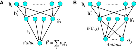
Figure 2. Neural implementation of belief-based value estimation and action selection. (A) Value estimation network. Input to the network is a belief state vector b_t and the output is an estimate of its value. The denote learned “belief points” which are the “centers” or means of the Gaussian basis functions g_i. The can be interpreted as synaptic weights (see text). (B) Action selection network.

The input layer receives the belief state b_t as input from the belief computation network discussed above. The hidden layer represents a set of Gaussian “basis” functions whose centers (means) denote a set of belief points. Each hidden layer neuron i is activated in proportion to how close the current input belief state is to its preferred belief point :

where g_i(b_t) denotes the firing rate of the ith hidden layer neuron, ||x|| denotes the square root of the sum of squared elements of vector x, and σ² is a variance parameter.

The belief points can be regarded as synaptic weights from the input layer to hidden neuron i. To see this, note that the output g_i(b_t) of each hidden layer neuron i is computed using an exponential activation function whose input is given by where c is a constant and l is also a constant if b_t and are normalized to be of constant length in the network. Thus, in effect, each belief point acts multiplicatively on the input b_t in the same manner as a traditional synaptic weight vector. These synaptic weight vectors (“basis belief points”) can be learned from input beliefs b_t as described below.

The output of the network is given by:

where v_i is the synaptic weight from hidden layer neuron i to the output neuron (we assume a single output neuron in the model, though this can be generalized to a distributed representation of value using multiple output neurons).

The synaptic weights v_i and can be learned by performing gradient descent at each time step on the following error function based on Eq. (5), after substituting for V^π:

The synaptic weights at time t are adapted according to:

where α₁ and α₂ are constants governing the rate of learning, and δ_{t + 1} is the TD error . It can be seen that both sets of synaptic weights are adapted in proportion to the TD error . However, unlike previous models, TD learning here is based on belief states.

A more interesting observation is that the learning rule (7) for the belief basis vectors is similar to traditional unsupervised competitive learning rules (e.g., self-organizing maps; Haykin, 2008) where a weight vector (or “prototype vector” in competitive learning parlance) is changed in proportion to how similar it is to an input (“soft competition”; cf. the term). However, unlike traditional unsupervised learning, learning here is also influenced by rewards and value due to the presence of the TD error term δ_{t + 1} in the learning rule. The learned basis vectors therefore do not simply capture the statistics of the inputs but do so in a manner that minimizes the error in prediction of value.

Neural computation of actions

The network for action selection (Figure 2B) is similar to the value estimation network. Although in general the action selection network could use a separate set of input-to-hidden layer basis vectors, we assume for the sake of parsimony that the same input-to-hidden layer basis vectors (belief points) are used by the value and action selection networks. The output layer of the action selection network represents the set of K possible actions, one of which is selected probabilistically at a given time step. Making action selection probabilistic allows the model to explore the reward space during the early phase of learning and to remain sensitive to non-stationary elements of the environment such as changes in reward contingencies.

In the model, the probability of choosing action a_j for an input belief b_t is given by:

where W(i,j) represents the synaptic weight from hidden neuron i to output neuron j and Z is the normalization constant. The parameter λ governs the degree of competition: as λ approaches 0, action selection approaches a winner-take-all mode; larger values of λ allow more diverse selection of actions, permitting exploration. In the simulations, we used a fixed value of λ to allow a small amount of exploration at any stage in the learning process. The action selection model described above leads to a relatively simple learning rule for W (see below), but we note here that other probabilistic action selection methods could potentially be used as well.

We now derive a simple learning rule for the action weights W. Suppose that the action a_j has just been executed. If the action results in an increase in value (i.e., positive TD error δ_{t + 1}), we would like to maximize the probability P(a_j|b_t); if it causes a decrease in value (negative TD error δ_{t + 1}), we would like to minimize P(a_j|b_t). This is equivalent to maximizing P(a_j|b_t)when δ_{t + 1} is positive and maximizing 1/P(a_j|b_t) when δ_{t + 1} is negative. The desired result can therefore be achieved by maximizing the function or equivalently, maximizing , which is equal to δ_{t + 1} log P(a_j|b_t). Thus, we would like to find a set of weights W(i,j)* such that:

Substituting Eq. (8) into Eq. (9) and ignoring the normalization constant log Z, we obtain the function:

An approximate solution to the optimization problem in (9) can be obtained by performing gradient ascent on J_t, resulting in the following learning rule for W(i,j) when an action a_j was executed at time t (α₃ here is the learning rate):

In other words, after an action a_j is chosen and executed, the weights W(i,j) for that action are adapted in proportion to δ_{t + 1}g_i(b_t) which is the TD error weighted by the corresponding hidden neuron’s firing rate. This has the desired effect of increasing the probability of an action if it resulted in an increase in value (positive TD error) and decreasing the probability if it caused a decrease in value (negative TD error). The rule for learning actions can therefore be seen as implementing Thorndike’s well-known “law of effect” in reinforcement learning (Thorndike, 1911).

Mapping the Model to Neuroanatomy

We postulate that the probabilistic computation of beliefs in Eq. (2) is implemented within the recurrent circuits of the neocortex. Support for such a hypothesis comes from experimental studies suggesting that perception and action involve various forms of Bayesian inference, at least some of which may be implemented in the neocortex (see, for example, review chapters in Rao et al., 2002; Doya et al., 2007).

We further postulate that the outputs of cortical circuits (i.e., belief states) are conveyed as inputs to the basal ganglia, which implements the value and action selection networks in the model. In particular, we suggest that the striatum/STN-GPe-GPi/SNr network computes actions while the striatum-SNc/VTA network computes value (Figure 3). This is similar to “actor-critic” models of the basal ganglia (Barto, 1995; Houk et al., 1995), where the critic evaluates the value of the current world state and the actor selects an appropriate action. In contrast to this traditional model, the “critic” in our model evaluates the value of the current belief state rather than the world state (which is unavailable), and the “actor” selects actions based on the entire belief state.

FIGURE 3

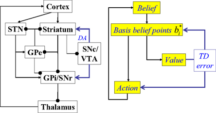
Figure 3. Suggested mapping of elements of the model to components of the cortex-basal ganglia network. STN, subthalamic nucleus; GPe, globus pallidus, external segment; GPi, Globus pallidus, internal segment; SNc, substantia nigra pars compacta; SNr, substantia nigra pars reticulata; VTA, ventral tegmental area; DA, dopaminergic responses. The model suggests that cortical circuits compute belief states, which are provided as input to the striatum (and STN). Cortico-striatal synapses are assumed to maintain a compact learned representation of cortical belief space (“basis belief points”). The dopaminergic responses of SNc/VTA neurons are assumed to represent reward prediction (TD) errors based on striatal activations. The GPe-GPi/SNr network, in conjunction with the thalamus, is assumed to implement action selection based on the compact belief representation in the striatum/STN.

In Figure 3, the input to the striatum consists of the outputs of various cortical areas which are assumed to represent belief states computed from sensory, motor, and limbic inputs. The striatum implements the hidden layer: the basis belief points are assumed to be learned in the cortico-striatal connections. The striatum-SNc/VTA network estimates the value , which is used to compute the TD prediction error . We postulate that the dopaminergic output from SNc/VTA represents this belief-based TD prediction error, which modulates the learning of belief points as well as the weights v_i and W.

The interpretation of dopaminergic outputs in the basal ganglia as representing prediction error is consistent with previous TD-based models of dopaminergic responses (Schultz et al., 1997). However, the model above further predicts that these responses are a function of the animal’s internally computed beliefs about a stimulus, rather than the stimulus itself. To test this prediction, one could vary the uncertainty associated with a stimulus and examine whether there are corresponding changes in the dopaminergic responses. Interestingly, results from such an experiment have recently been published by Nomoto et al. (2010). We compare their results to the model’s predictions in a section below.

Results

The Random Dots Task

We tested the neural POMDP model derived above in the well-known random dots motion discrimination task used to study decision making in primates (Shadlen and Newsome, 2001). We focus specifically on the reaction-time version of the task (Roitman and Shadlen, 2002) where the animal can choose to make a decision at any time. In this task, the stimulus consists of an image sequence showing a group of moving dots, a fixed fraction of which are randomly selected at each frame and moved in a fixed direction (for example, either left or right). The rest of the dots are moved in random directions. The fraction of dots moving in the same direction is called the motion strength or coherence of the stimulus.

The animal’s task is to decide the direction of motion of the coherently moving dots for a given input sequence. The animal learns the task by being rewarded if it makes an eye movement to a target on the left side of its fixation point if the motion is to the left, and to a target on the right if the motion is to the right. A wealth of data exists on the psychophysical performance of humans and monkeys on this task, as well as the neural responses observed in brain areas such as MT and LIP in monkeys performing this task (see Roitman and Shadlen, 2002; Shadlen and Newsome, 2001 and references therein).

Example I: Random Dots with Known Coherence

In the first set of experiments, we illustrate the model using a simplified version of the random dots task where the coherence value chosen at the beginning of the trial is known. This reduces the problem to that of deciding from noisy observations the underlying direction of coherent motion, given a fixed known coherence. We tackle the case of unknown coherence in a later section.

We model the task using a POMDP as follows: there are two underlying hidden states representing the two possible directions of coherent motion (leftward or rightward). In each trial, the experimenter chooses one of these hidden states (either leftward or rightward) and provides the animal with observations of this hidden state in the form of an image sequence of random dots at the chosen coherence. Note that the hidden state remains the same until the end of the trial. Using only the sequence of observed images seen so far, the animal must choose one of the following actions: sample one more time step (to reduce uncertainty), make a leftward eye movement (indicating choice of leftward motion), or make a rightward eye movement (indicating choice of rightward motion).

We use the notation S_L to represent the state corresponding to leftward motion and S_R to represent rightward motion. Thus, at any given time t, the state s_t can be either S_L or S_R (although within a trial, the state once selected remains unchanged). The animal receives noisy measurements or observations o_t of the hidden state based on P(o_t|s_t, c_t), where c_t is the current coherence value. We assume the coherence value is randomly chosen for each trial from a set {C₁, C₂,…, C_Q} of possible coherence values, and remains the same within a trial. At each time step t, the animal must choose from one of three actions {A_S, A_L, A_R} denoting sample, leftward eye movement, and rightward eye movement respectively.

The animal receives a reward for choosing the correct action, i.e., action A_L when the true state is S_L and action A_R when the true state is S_R. We model this reward as a positive number (e.g., between +10 and +30; here, +20). An incorrect choice produces a large penalty (e.g., between −100 and −400; here, −400) simulating the time-out used for errors in monkey experiments (Roitman and Shadlen, 2002). We assume the animal is motivated by hunger or thirst to make a decision as quickly as possible. This is modeled using a small negative reward (penalty of −1) for each time step spent sampling. We have experimented with a range of reward/punishment values and found that the results remain qualitatively the same as long as there is a large penalty for incorrect decisions, a moderate positive reward for correct decisions, and a small penalty for each time step spent sampling.

The transition probabilities P(s_t|s_{t − 1}, a_{t − 1}) for the task are as follows: the state remains unchanged (self-transitions have probability 1) as long as the sample action A_S is executed. Likewise, P(c_t|c_{t − 1,} A_S) = 1. When the animal chooses A_L or A_R, a new trial begins, with a new state (S_L or S_R) and a new coherence C_k (from {C₁, C₂,…, C_Q}) chosen uniformly at random.

In the first set of experiments, we trained the model on 6000 trials of leftward or rightward motion. Inputs o_t were generated according to P(o_t|s_t, c_t) based on the current coherence value and state (direction). For these simulations, o_t was one of two values O_L and O_R corresponding to observing leftward and rightward motion respectively. The probability P(o = O_L|s = S_L, c = C_k) was fixed to a value between 0.5 and 1 based on the coherence value C_k, with 0.5 corresponding to 0% coherence and 1 corresponding to 100%. The probability P(o = O_R|s = S_R, c = C_k) was defined similarly.

The belief state b_t over the unknown direction of motion was computed using a slight variant of Eq. (2) using the current input o_t, the known coherence value c_t = C_k, the known transition and observation models T and P(o_t|s_t,c_t), and the previous belief state:

The belief over S_L was computed as b_t(S_L) = 1−b_t(S_R). For the simulations described here, we used the above equation directly since our focus here is on how the value function and policy are learned, given belief states. A more sophisticated implementation could utilize one of the models for inference cited in the section Neural computation of belief, with the likelihood information provided by motion processing neurons in MT and recurrent connections implementing the feedback from the previous time step.

The resulting belief state vector b_t was fed as input to the networks in Figure 2. The basis belief points , value weights v_i, and action weights W were learned using the equations above (parameters: α₁ = α₃ = 0.0005, α₂ = 2.5 × 10⁻⁷, γ = 1, λ = 1, σ² = 0.05). The number of output units was three for the action network and one for the value network. A more realistic implementation could utilize populations of neurons to represent the two directions of motions and estimate posterior probabilities from population activity; for simplicity, we assume here that the two posterior probabilities are represented directly by two units.

The number of hidden units used in the first set of simulations was 11. We found that qualitatively similar results are obtained for other values. The number of hidden units determines the precision with which the belief space can be partitioned and mapped to appropriate actions. A complicated task could require a larger number of hidden neurons to partition the belief space in an intricate manner for mapping portions of the belief space to the appropriate value and actions.

The input-to-hidden weights were initialized to evenly span the range between [0 1] and [1 0]. Similar results were obtained for other choices of initial parameters (e.g., uniformly random initialization).

Learning to solve the task

The process of learning is captured in Figure 4, which shows the total reward received over the last 500 time steps as a function of time. As seen in the plot, learning is rapid over the first 1500 or so time steps before the amount of reward received fluctuates around an approximately stable value. Although 1500 time steps may seem large, it should be remembered that a trial can last between a few to several hundred time steps; therefore, 1500 time steps actually span a reasonably small number of motion trials.

FIGURE 4

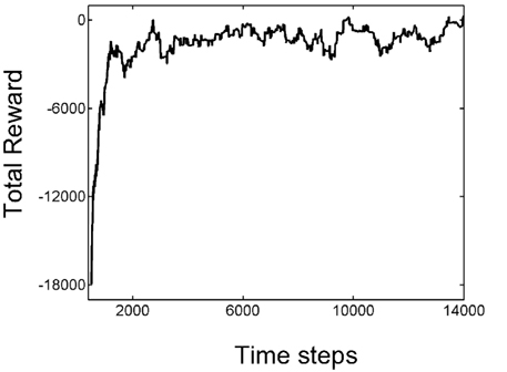
Figure 4. Learning the random dots task. The plot shows the total reward received over the last 500 time steps as a function of the number of time steps encountered thus far. Note the rapid increase in total reward in the first 1500 or so times steps as a result of trial-and-error learning, followed by slower convergence to an approximately stable value near 0.

Figure 5 shows the value function learned by the value estimation network for input belief states before and after learning (left and right panels respectively).

FIGURE 5

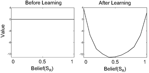
Figure 5. Learning values for beliefs in the value estimation network. The plots show the value for belief over the S_R (rightward motion) state. The full belief state is simply [Belief(S_R) 1-Belief(S_R)]. Before learning begins, all values for belief states are initialized to 0 (left panel). After learning, highly uncertain belief states (Belief(S_R) near 0.5) have low value while belief states near 0 or 1 (high certainty about states S_L or S_R respectively) have high values.

Before learning, all values are 0 because the weights v_i are initialized to 0. After learning, the network predicts a high value for belief states that have low uncertainty. This is because at the two extremes of belief, the hidden state is highly likely to be either S_L (belief(S_R) near 0) or S_R (belief(S_R) near 1). In either case, selecting the appropriate action (as in Figure 6) results in a large positive reward on average. On the other hand, for belief values near 0.5, uncertainty is high – further sampling is required to reduce uncertainty (each sample costing −1 per time step). Choosing A_L or A_R in these uncertain belief states has a high probability of resulting in an incorrect choice and a large negative reward. Therefore, belief states near [0.5 0.5] have a much lower value compared to belief states near [0 1] or [1 0].

FIGURE 6

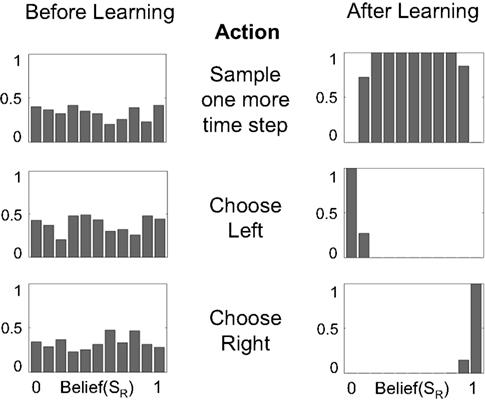
Figure 6. Mapping beliefs to actions: policy learning in the action selection network. The plots depict the probability of choosing the sample, left, or right actions (A_S, A_L, A_R) as a function of belief for state S_R (rightward motion). The “Sample” action is chosen with high probability when the current state is uncertain (belief is between 0.2 and 0.8, top right plot). The “Choose Left” action has a high probability when the belief for S_R is near 0 (i.e., the belief for S_L is high) and the “Choose Right” action when belief for S_R is near 1.

Learning actions

Figure 6 shows the policy learned by the action selection network based on the TD prediction error produced by the value estimation network. Starting from uniform probabilities (Figure 6, left panels), the network selects the “Sample” action A_S with high probability when there is uncertainty in the belief state about the true hidden state (Figure 6, top right panel). The “Sample” action thus helps to decrease this uncertainty by allowing more evidence to be gathered. The network chooses the Left or Right action only when the belief for S_R is close to 0 or 1, i.e., the true state is highly likely to be S_L or S_R respectively (Figure 6, lower right panels).

Performance of the trained network

The performance of the model on the task depends on the coherence of the stimulus and is quantified by the psychometric function in Figure 7 (left panel). For comparison, the psychometric function for a monkey performing the same task (Roitman and Shadlen, 2002) is shown in the right panel. A sigmoid function (cumulative Weibull) was used to fit the data points in both plots. Performance in the model varies from chance (50% correct) to 100% correct as motion strength is increased from 0 to 100%.

FIGURE 7

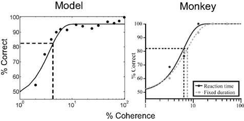
Figure 7. Performance of the model: psychometric function. The plots show performance accuracy as a function of motion coherence for the model (left) and a monkey (data from Roitman and Shadlen, 2002). A sigmoid (cumulative Weibull) function was fit to the data in both cases and the psychophysical threshold (coherence achieving 82% accuracy) was calculated (dotted lines). (Note: only the reaction time, not the fixed duration version of the task, is considered in this article).

Accuracies above 90% are already achieved for coherences 8% and above, similar to the monkey data. 100% accuracy in the model is consistently achieved only for the 100% coherence case due to the probabilistic method used for action selection (see section Neural computation of actions); the value of the action selection parameter λ could be decreased after learning to obtain a winner-take-all scheme with less stochasticity.

The vertical dotted line in each plot in Figure 7 indicates the psychophysical threshold: the motion coherence that yields 82% accuracy (as given by horizontal dotted line). This threshold was approximately 4.3% coherence in the model (in the monkey, this is 6.8%; Figure 7, right panel). The threshold in the model is a function of the parameters used for the networks and for learning.

We did not attempt to quantitatively fit a particular monkey’s data, preferring to focus instead on qualitative matches. It should be noted that the model learns to solve the random dots task from scratch over the course of several hundred trials, with the only guidance provided being the reward/penalty at the end of a trial. This makes fitting curves, such as the psychometric function, to a particular monkey difficult, compared to previous models of the random dots task that are not based on learning and which therefore allow easier parameter fitting.

Figure 8 (left panel) shows the mean reaction time for correct choices as a function of motion coherence, along with a straight line fit from least squares regression. As expected, stimuli with low motion coherence require longer reaction times (more sampling actions) than high coherence stimuli, the average reaction time ranging from about 680 time steps (2% coherence) to less than 10 time steps (37% coherence and above). The reaction time data for the same monkey as in Figure 7 is shown in Figure 8 (right panel).

FIGURE 8

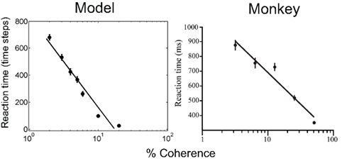
Figure 8. Performance of the model: reaction time. The plots show reaction time for correct trials as a function of motion coherence for the model (left) and a monkey (data from Roitman and Shadlen, 2002). A least squares straight line fit to the data in semilog coordinates is shown in both cases.

LIP responses as beliefs

The learned policy in Figure 6 predicts that the model should select the “Sample” action to decrease uncertainty about the stimulus until the posterior probability (belief) for one of the two states S_L or S_R reaches a high value, at which point the appropriate action A_L or A_R is selected. With such a policy, if the true state is, for example, S_L, the belief for S_L would rise in a random walk-like fashion as “Sample” actions are executed and new observations made, until the belief reaches a high value near 1 when A_L is selected with high probability.

Figure 9 (left panel) shows the responses of a model neuron representing the belief for S_L over time for stimuli of different coherences (solid traces are cases where the underlying state was S_L, dashed traces are cases where the underlying state was S_R). As expected from the reaction time data, the belief responses show a direct dependence on stimulus coherence, with a faster rate of increase in belief for higher coherence values (solid traces). This faster rate of growth arises because each observation provides evidence in proportion to the likelihood P(o_t|s_t, c_t), which is larger for higher coherence values. The faster rate of growth in belief, as illustrated in Figure 9, manifests itself as faster reaction times for high coherence stimuli (Figure 8).

FIGURE 9

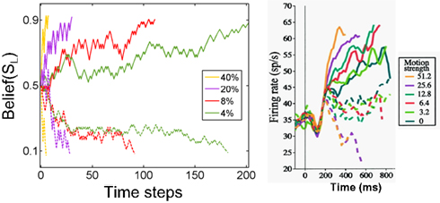
Figure 9. Belief computation in the model compared to LIP responses. The plot on the left shows responses of a model neuron representing belief (posterior probability) for leftward motion (state S_L) for stimuli moving leftward (solid) and rightward (dashed) with motion coherences 4, 8, 20, and 40% respectively. The model chose the correct action in each case. The panel on the right shows average responses of 54 neurons in cortical area LIP in a monkey (figure adapted from Roitman and Shadlen, 2002). The solid lines are for motion in the direction preferred by the neuron and dashed lines are for motion in the opposite direction. Belief responses in the model exhibit a random walk-like ramping behavior similar to LIP responses, with faster rates of growth for higher coherence values.

The random walk-like ramping behavior of the belief computing neurons in the model is comparable to the responses of cortical neurons in area LIP in the monkey (Figure 9, right panel) (Roitman and Shadlen, 2002). The model thus posits that LIP responses are proportional to or a direct function of belief (posterior probability) over a particular task-relevant variable.¹

Unlike previous models of LIP responses, the POMDP model suggests an interpretation of the LIP data in terms of maximizing total expected future reward within a general framework for probabilistic reasoning under uncertainty. Thus, parameters such as the threshold for making a decision emerge naturally within the POMDP framework as a result of maximizing reward. As the model responses in Figure 9 illustrate, the threshold for the particular implementation of the model presented in this section is around 0.9. This is not a fixed threshold because action selection in the model is stochastic – actions are selected probabilistically (see section Neural computation of actions): there is a higher probability that a terminating action (A_L or A_R) will be selected once the belief values are near 0.9 or above.

Learning of belief states: a role for the cortico-striatal pathway

The hidden layer neurons in Figure 2 learn basis functions in their synaptic weights to represent input beliefs from the belief computation network. These neurons thus become selective for portions of the belief space that are most frequently encountered during decision making and that help maximize reward, as prescribed by the learning rule in Eq. (7).

Since the belief vector is continuous valued and typically high-dimensional, the transformation from the input layer to hidden layer in Figure 2 can be regarded as a form of dimensionality reduction of the input data. The hidden layer neurons correspond to striatal neurons in the model (Figure 3). Thus, the model suggests a role for the cortico-striatal pathway in reducing the dimensionality of cortical belief representations, allowing striatal neurons to efficiently represent cortical beliefs in a compressed form. Interestingly, Bar-Gad et al. (2003) independently proposed a reinforcement-driven dimensionality reduction role for the cortico-striatal pathway but without reference to belief states. Simultaneously, in the field of artificial intelligence, Roy et al. (2005) proposed dimensionality reduction of belief states (they called it “belief compression”) as an efficient way to solve large-scale POMDP problems.

Figure 10 shows examples of learned hidden layer representations of the belief space for two different motion coherences. Figure 10A shows samples of input beliefs when motion coherence is fixed to 30%. These beliefs are received as inputs by the value estimation and action selection networks in Figure 2 during learning.

FIGURE 10

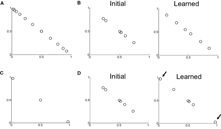
Figure 10. Learning of belief basis functions in the model. (A) Samples of input beliefs for a set of trials where motion coherence was set to 30%. (B) (Left) Initial randomly selected basis belief points in the network (input to hidden layer weights). (Right) Belief basis points learned by the network for predicting value for the belief distribution in (A). Note that learning has caused the belief points to spread out so as to sufficiently capture the input belief distribution shown in (A) to predict value. (C) Distribution of input beliefs when motion coherence is set to 95%. (D) (Left) Initial randomly selected basis belief points (same as in B left panel). (Right) Basis belief points after learning. The arrows indicate the two belief points that underwent the most change from their initial values – these now lie at the two extremes to better approximate the input distribution of beliefs in (C) and more accurately predict value.

When initialized to random values (Figure 10B, left panel), the input-to-hidden layer weights adapt to the input distribution of beliefs according to Eq. (7) and converge to the values shown in Figure 10B (“Learned”). These learned “belief points” span a wider range of the belief space to better approximate the value function for the set of possible input beliefs in Figure 10A. When motion coherence is fixed to a very high value (95%), the input belief distribution is sparse and skewed (Figure 10C). Learning in this case causes two of the weight values to move to the two extremes of the belief space (arrows in Figure 10D) in order to account for the input beliefs in this region of belief space in Figure 10C and better predict value. The remaining belief points are left relatively unchanged near the center of the belief space due to the sparse nature of the input belief distribution in this case.

Dopamine and reward prediction error

The anatomical mapping of elements of the model to basal ganglia anatomy in Figure 3 suggests that reward prediction error (i.e., the TD error) in the model could correspond to dopaminergic (DA) signals from SNc and VTA. This makes the proposed model similar to previously proposed actor-critic models of the basal ganglia (Barto, 1995; Houk et al., 1995) and TD models of DA responses (Schultz et al., 1997). One important difference however is that value in the present model is computed over belief states. This difference is less important for simple instrumental conditioning tasks such as those that have typically been used to study dopaminergic responses in the SNc/VTA (Mirenowicz and Schultz, 1994). In these experiments, monkeys learn to respond to a sound and press a key to get a juice reward. The degree of uncertainty about the stimulus and reward is small, compared to the random dots task.

We first present a comparison of model TD responses to DA responses seen in the simple conditioning task of (Mirenowicz and Schultz, 1994). In a subsequent section, we present comparisons with DA responses for the random dots task.

To illustrate TD responses in the model for simple conditioning, we reduced the uncertainty in the random dots task to 0 and tracked the evolution of the TD error. Figure 11A shows the TD error in the model during the course of learning with motion coherence set to 100%. Before training (t = 1), the TD error at the start of the trial is 0 (values initialized to 0) and at the end of the trial, this error is equal to the reward (+20) because the value predicted is 0. As learning proceeds, the predicted value (Eq. 6) becomes increasingly accurate and the TD error at the end of the trial decreases (Figure 11A; trials at t = 1000 and 2500) until it becomes approximately 0 (t = 6500), indicating successful prediction of the reward. Simultaneously, as a consequence of TD learning, the value for the belief state at the start of the trial is now equal to the reward (since reward is assured on every trial for the 100% coherence case, once the correct actions have been learned). Thus, after learning, the TD error at the start of the trial is now positive and equal to the amount of expected reward (+20) (see Figure 11A, last panel).

FIGURE 11

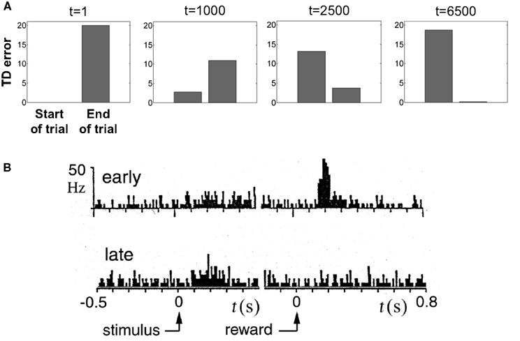
Figure 11. Reward prediction (TD) error during learning. (A) Evolution of TD error in the model during the course of learning the belief-state-to-action mapping for the 100% coherence condition (no stimulus uncertainty). Before learning (t = 1), TD error is large at the end of the trial and 0 at the start. After learning, the error at the end of the trial is reduced to almost 0 (t = 6500) while the error at the start is large. (B) Dopamine response in a SNc/VTA neuron hypothesized to represent reward prediction errors (adapted from Mirenowicz and Schultz, 1994). Before learning (“early”), the dopamine response is large at the end of the trial following reward delivery. After learning (“late”), there is little or no response at the end of the trial but a noticeable increase in response at the start of the trial after presentation of the stimulus. Compare with t = 1 and t = 6500 in (A).

This behavior of the TD error in the model (Figure 11A) is similar to phasic DA responses in SNc/VTA as reported by Schultz and colleagues (Figure 11B) for their simple instrumental conditioning task (Mirenowicz and Schultz, 1994). The interesting issue of how the TD error changes as stimulus uncertainty is varied is addressed in a later section.

Example II: Random Dots Task with Unknown Coherence

In the previous section, we considered the case where only motion direction was unknown and the coherence value was given in each trial. This situation is described by the graphical model (Koller and Friedman, 2009) in Figure 12A, where d_t represents the direction of motion at time t, c_t the coherence, o_t the observation, and a_t the action. The simulations in the previous section assumed motion direction d_t is the sole hidden random variable; the values for the other variables (except a_t) were given. The action a_t was obtained from the learned policy based on the belief over d_t.

FIGURE 12

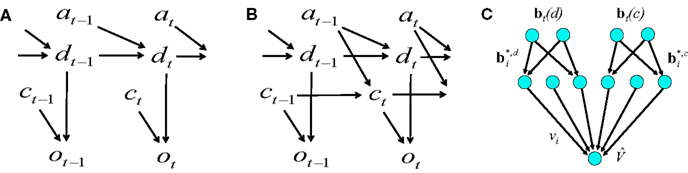
Figure 12. Probabilistic graphical models and value estimation network for the random dots task. (A) Graphical model used for the case of known coherence. The hidden variable is motion direction d_t while the coherence c_t, observation o_t, and the previously executed action a_t-1 are assumed to be known. The action a_t is obtained from the learned policy based on the belief over d_t. (B) Graphical model used for the case of unknown coherence. The hidden variables include motion direction d_t and coherence c_t. The value function and policy are computed based on belief over both d_t and c_t. (C) Network for value estimation. Belief basis points and are learned separately for the two hidden variables d_t and c_t, but activations of all hidden units are combined to predict the value .

We now examine the case where both the direction of motion and coherence are unknown. The graphical model is shown in Figure 12B. The only known variables are the observations up to time t and the actions up to time t − 1. This corresponds more closely to the problem faced by the animal.

Suppose d_t can be one of the values in {1, 2,…, N} (each number denotes a direction of motion; the two-alternative case corresponds to the values 1 and 2 representing leftward and rightward motion respectively). Similarly, c_t can be one of {1, 2, …, Q}, each representing a particular coherence value.

Then, the belief state at time t is given by:

This belief state can be computed as in Eq. (2) by defining the transition probabilities jointly over d_t and c_t. The belief over d_t and c_t can then computed by marginalizing:

Alternatively, one can estimate these marginals directly by performing Bayesian inference over the graphical model in Figure 12B using, for example, a local message-passing algorithm such as belief propagation (Pearl, 1988) (see Rao, 2005, for a possible neural implementation). This has the advantage that conditional independencies between variables (such as d_t and c_t) can be exploited, allowing the model to scale to larger scale problems.

Figure 12C shows the value estimation network used to learn the POMDP policy. Note that the output value depends on both the belief over direction as well as belief over coherence. Separate belief basis points are learned for the two types of beliefs. A similar network is used for learning the policy, but with hidden-to-output connections analogous to Figure 2B. The fact that the two types of beliefs are decoupled makes it easier for the network to discover over the course of the trials that the reward depends on determining the correct direction, irrespective of coherence value.

To illustrate this model, we simulated the case where there are two directions of motion (N = 2) denoted by L and R, corresponding to leftward and rightward motion respectively, and two coherence values (Q = 2) denoted by E and H, corresponding to an “Easy” coherence (60%) and a “Hard” coherence (8%) respectively.

The model was exposed to 4000 trials, with the motion direction and coherence selected uniformly at random for each trial. The rewards and penalties were the same as in the previous section (+20 reward for correct decisions, −400 for errors, and −1 for each sampling action). The number of hidden units, shared by the value and action networks, was 25 each for belief over direction and coherence. The other parameters were set as follows: α₁ = 3 × 10⁻⁴, α₂ = 2.5 × 10⁻⁸, α₃ = 4 × 10⁻⁶, γ = 1, λ = 0.5, σ² = 0.05.

Figure 13A shows the learned value function as a joint function of belief over coherence (E = “Easy”) and belief over direction (L = “Left”). The value function is ‘U’ shaped as a function of belief over direction, similar to Figure 5 for the known coherence case, signifying again that higher value is attached to highly certain belief about direction. More interestingly, the overall value decreases as belief in coherence goes from “Easy” (Belief(E) = 1) to “Hard” (Belief(E) = 0), signifying a greater expected reward for an “Easy” trial compared to a “Hard” trial. This observation is depicted more explicitly in Figures 13B,C.

FIGURE 13

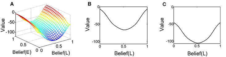
Figure 13. The learned value function. (A) The learned value as a joint function of beliefs over coherence (E = “Easy”) and direction (L = “Left”). The Belief(E) axis represents the belief (posterior probability) that the current trial is an “Easy” coherence trial (i.e., coherence = 60%). The Belief(L) axis represents the belief that the motion direction is Leftward. Note the overall decrease in value as Belief(E) falls to 0, indicating a “Hard” trial (coherence = 8%). (B,C) Two slices of the value function in (A) for Belief(E) = 1 and 0 respectively. There is a drop in overall value for the hard coherence case (C). Also note the similarity to the learned value function in Figure 5 for the known coherence case.

The corresponding learned policy is shown in Figure 14. As in Figure 6, the policy advocates sampling when there is uncertainty in the two types of beliefs but the choice of Left or Right action depends on the belief in a particular direction crossing an approximate threshold, regardless of whether coherence value is “Hard” or “Easy” (Figures 14B,C). The model was thus correctly able to discover the dependence of reward on direction and the lack of dependence on coherence value (“Hard” or “Easy”).²

FIGURE 14

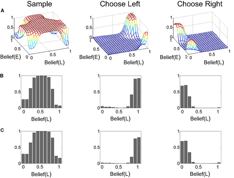
Figure 14. The learned policy. (A) The learned policy as a joint function of beliefs over coherence (E = “Easy”) and direction (L = “Left”). The policy advocates sampling when there is uncertainty in beliefs and chooses the appropriate action (Left/Right) when belief in a particular direction crosses an approximate threshold. (B,C) The policy function in (A) for Belief(E) = 1 and 0 respectively. The policies for these two special cases are similar to the one for the known coherence case (Figure 6).

Figure 15 (left panel) shows the temporal evolution of beliefs for example trials with 60% and 8% coherence (“Easy” and “Hard” trials). The belief trajectory over direction (the marginal posterior probability) resembles LIP responses in the monkey (compare with Figure 9).

FIGURE 15

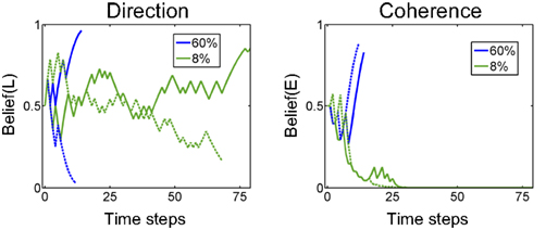
Figure 15. Examples of belief computation. The plots show examples of the evolution of belief state over time for 60% coherence (blue) and 8% coherence (green). Belief(L) denotes belief that motion direction is Leftward. Belief(E) is the belief that the current trial is an “Easy” coherence trial (coherence = 60%). The solid lines represent a trial in which motion was in the leftward direction while dotted lines represent a rightward motion trial.

The belief trajectory over coherence in Figure 15 (right panel) shows that the model can correctly infer coherence type (“Easy” or “Hard”) for both directions of motion. Interestingly, for the “Hard” trials (8% coherence), the model’s belief that the trial is “Hard” converges relatively early (green solid and dashed lines in Figure 15 (right panel), showing Belief(E) going to 0), but the model commits to a Left or Right action only when belief in a direction reaches a high enough value.

Comparison with Dopamine Responses In the Random Dots Task

In this section, we compare model predictions regarding reward prediction error (TD error) with recently reported results on dopamine responses from SNc neurons in monkeys performing the random dots task (Nomoto et al., 2010).

We first describe the model’s predictions. Consider an “Easy” coherence trial where the direction of motion is leftward (L). The model starts with a belief state of [0.5 0.5] over direction (and coherence); subsequent updates push Belief(L) higher, which corresponds to climbing the ramp in the value function in Figure 13A. The TD error tracks the differences in value as we climb this ramp. For an “Easy” trial, one might expect large positive TD errors as the belief rapidly goes from [0.5 0.5] to higher values (see solid blue belief trace in Figure 15) with smaller but positive TD errors (on average) as the decision threshold approaches.

Figure 16A (left panel) shows this prediction for the model learned in the previous section (for the unknown coherence and direction case). The plot shows how reward prediction (TD) error in the model evolves over time in “Easy” motion coherence trials (coherence = 60%). The TD error shown was averaged over correct trials in a set of 1000 trials containing a uniformly random mixture of “Easy” and “Hard” trials. An arbitrary delay of four time steps from motion onset at 0 was used for visualization in the plot, with TD error assumed to be 0 for these time steps. As predicted, the average TD error is large and positive initially, and gradually decreases to 0.

FIGURE 16

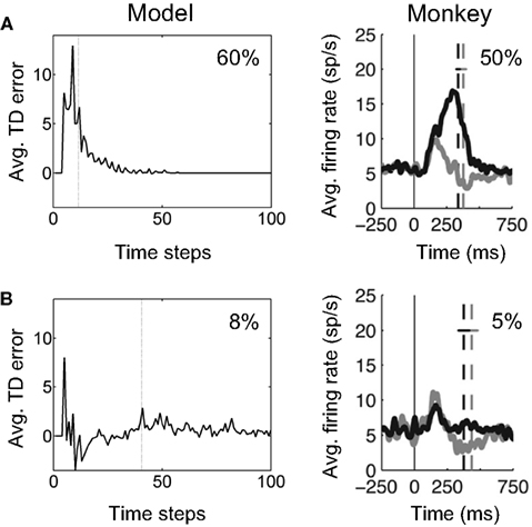
Figure 16. Reward prediction error and dopamine responses in the random dots task. (A) The plot on the left shows the temporal evolution of reward prediction (TD) error in the model, averaged over trials with “Easy” motion coherence (coherence = 60%). The dotted line shows the average reaction time. The plot on the right shows the average firing rate of dopamine neurons in SNc in a monkey performing the random dots task at 50% motion coherence. The dashed line shows average time of saccade onset. The gray trace and line show the case where the amount of reward was reduced (not modeled here; see Nomoto et al., 2010). (B) (Left) Reward prediction (TD) error in the model averaged over trials with “Hard” motion coherence (coherence = 8%). (Right) Average firing rate of the same dopamine neurons as in (A) but for trials with 5% motion coherence. (Dopamine plots adapted from Nomoto et al., 2010).

For comparison, Figure 16A (right panel) shows the average firing rate of 35 dopamine neurons in SNc in a monkey performing the random dots task for 50% motion coherence trials (data from Nomoto et al., 2010). Nomoto et al. present results from two monkeys (K and L) and report an initial dopamine response that is independent of trial type (direction and coherence) and a later response that depends on trial type.³ In the data in Figure 16A (right panel), which is from their monkey K, the initial response includes the smaller peak occurring before 200 ms; the trial-type dependent response is the rest of the response including the larger peak. The model suggests an explanation for this trial-type dependent part of the response.

For “Hard” motion coherence trials (coherence = 8%), the average TD error in the model is shown in Figure 16B (left panel). The model predicts an initial positive response followed by a negative prediction error on average due to the “Hard” trial. Figure 16B (right panel) shows the average firing rate for the same dopamine neurons as Figure 16A but for trials with 5% motion coherence. The trial-type dependent response is noticeably smaller than for the 50% coherence case, as predicted by the model. The negative part of the prediction error is not as apparent in the black trace in Figure 16B, although it can be seen in the gray trace (small-reward condition).

The model also predicts that upon reward delivery at the end of a correct trial, TD error should be larger for the “Hard” (8% coherence) case due to its smaller expected value (see Figure 13). This prediction is shown in Figure 17A. In the monkey experiments (Nomoto et al., 2010), after the monkey had made a decision, a feedback tone was presented: a high-pitch tone signaled delivery of reward after the tone (i.e., a correct trial) and a low-pitch tone signaled no reward (error trial). The tone type thus acted as a sure indicator of reward. Figure 17B shows the population dopamine response of the same SNc neurons as in Figure 16 but at the time of the reward tone for correct trials (black trace). As predicted by the model, the dopamine response after reward tone is larger for lower coherences.

FIGURE 17

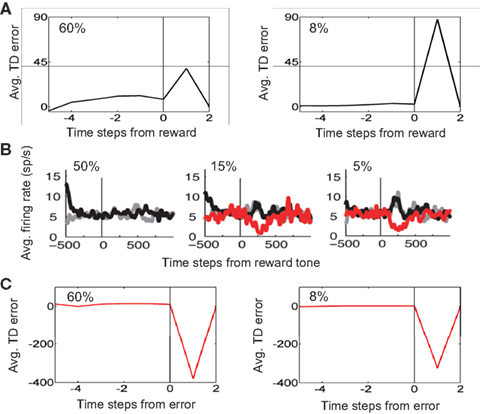
Figure 17. Reward prediction error at the end of a trial. (A) Average reward prediction (TD) error at the end of correct trials for the 60% coherence case (left) and the 8% coherence case (right). The vertical line denotes the time of reward delivery. Right after reward delivery, TD error is larger for the 8% coherence case due to its smaller expected value (see Figure 13). (B) Population dopamine responses of SNc neurons in the same monkey as in Figure 16 but after the monkey has made a decision and a feedback tone indicating reward or no reward is presented. (Plots adapted from Nomoto et al., 2010). The black and red traces show dopamine response for correct and error trials respectively. The gray traces show the case where the amount of reward was reduced (see (Nomoto et al., 2010) for details). (C) Average reward prediction (TD) error at the end of error trials for the 60% coherence case (left) and the 8% coherence case (right). The absence of reward (or negative reward/penalty in the current model) causes a negative reward prediction error, with a slightly larger error for the higher coherence case due to its higher expected value (see Figure 13).

Finally, in the case of an error trial, the model predicts that the absence of reward (or presence of a negative reward/penalty as in the simulations) should cause a negative reward prediction error and this error should be slightly larger for the higher coherence case due to its higher expected value (see Figure 13). This prediction is shown in Figure 17C, which compares average reward prediction (TD) error at the end of error trials for the 60% coherence case (left) and the 8% coherence case (right). The population dopamine responses for error trials are depicted by red traces in Figure 17B.

Example III: Decision Making Under a Deadline

Our final set of results illustrates how the model can be extended to learn time-varying policies for tasks with a deadline. Suppose a task has to be solved by time T (otherwise, a large penalty is incurred). We will examine this situation in the context of a random dots task where the animal has to make a decision by time T in each trial (in contrast, both the experimental data and simulations discussed above involved the dots task with no deadline).

Figure 18A shows the network used for learning the value function. Note the additional input node representing elapsed time t, measured from the start of the trial. The network includes basis neurons for elapsed time, each neuron preferring a particular time . The activation function is the same as before:

where is a variance parameter. In the simulations, was set to progressively larger values for larger loosely inspired by the fact that an animal’s uncertainty about time increases with elapsed time (Leon and Shadlen, 2003). Specifically, both and were set arbitrarily to 1.25ⁱ for i = 1,…, 65. The number of hidden units for direction, coherence, and time was 65. The deadline T was set to 20 time steps, with a large penalty (−2000) if a left/right decision was not reached before the deadline. Other parameters included: +20 reward for correct decisions, −400 for errors, −1 for each sampling action, α₁ = 2.5 × 10⁻⁵, α₂ = 4 × 10⁻⁸, α₃ = 1 × 10⁻⁵, γ = 1, λ = 1.5, σ² = 0.08. The model was trained on 6000 trials, with motion direction (Left/Right) and coherence (Easy/Hard) selected uniformly at random for each trial.

FIGURE 18

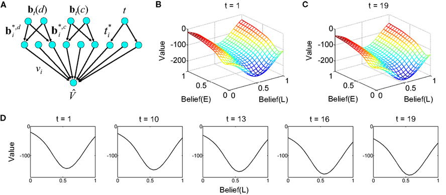
Figure 18. Decision making under a deadline. (A) Network used for learning value as a function of beliefs and elapsed time. The same input and hidden units were used for the action selection network (not shown). (B,C) Learned value function for time t = 1 and t = 19 within a trial with deadline at t = 20. Axis labels are as in Figure 13A. Note the drop in overall value in (C) for t = 19. The progressive drop in value as a function of elapsed time is depicted in (D) for a slice through the value function at Belief(E) = 1.

Figures 18B,C show the learned value function for the beginning (t = 1) and near the end of a trial (t = 19) before the deadline at t = 20. The shape of the value function remains approximately the same, but the overall value drops noticeably over time. Figure 18D illustrates this progressive drop in value over time for a slice through the value function at Belief(E) = 1.

The learned policy, which is a function of elapsed time, is shown in Figure 19. For the purposes of illustration, only the portion of the policy for hard coherence (specifically, for Belief(E) = 0) is shown, but the policy learned by the model covers all values of Belief(E).

FIGURE 19

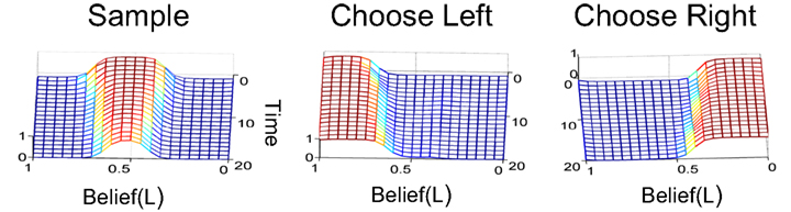
Figure 19. Collapsing decision threshold in the model. The learned policy as a joint function of elapsed time and belief over direction (L = “Left”), shown here for Belief(E) = 0. The trial begins at time 0, with a deadline at time 20 when the trial is terminated. Compare with the learned policies in Figures 6 and 14. Note the gradual decrease in threshold over time for choosing a Left/Right action, a phenomenon that has been called a “collapsing” bound in the decision making literature (e.g., Churchland et al., 2008).

As seen in Figure 19, during the early phase of a trial, the “Sample” action is preferred with high probability; the “Choose Left” action is chosen only if Belief(L) exceeds a high threshold (conversely for “Choose Right”). Such a policy is similar to the ones we encountered before in Figures 6 and 14 for the deadline-free case.

More interestingly, as we approach the deadline, the threshold for the “Choose Left” action collapses to a value close to 0.5 (and likewise for “Choose Right”), suggesting that the model has learned it is better to pick one of these two actions (at the risk of committing an error) than to reach the deadline and incur a larger penalty. Such a “collapsing” bound or decision threshold has also been predicted by previous theoretical studies (e.g., Latham et al., 2007; Frazier and Yu, 2008) and has found some experimental support (Churchland et al., 2008).

Conclusions

The mechanisms by which animals learn to choose actions in the face of uncertainty remains an important open problem in neuroscience. The model presented in this paper proposes that actions are chosen based on the entire posterior distribution over task-relevant states (the “belief state”) rather than a single “optimal” estimate of the state. This allows an animal to take into account the current uncertainty in its state estimates when selecting actions, permitting the animal to perform information gathering actions for reducing uncertainty and choosing overt actions only when (and if) uncertainty is sufficiently reduced.

We formalized the proposed approach using the framework of partially observable Markov decision processes (POMDPs) and presented a neural model for solving POMDPs. The model relies on TD learning for mapping beliefs to values and actions. We illustrated the model using the well-known random dots task and presented results showing that (a) the temporal evolution of beliefs in the model shares similarities with the responses of cortical neurons in area LIP in the monkey, (b) the threshold for selecting overt actions emerges naturally as a consequence of learning to maximize rewards, (c) the model exhibits psychometric and chronometric functions that are qualitatively similar to those in monkeys, (d) the time course of reward prediction error (TD error) in the model when stimulus uncertainty is varied resembles the responses of dopaminergic neurons in SNc in monkeys performing the random dots task, and (e) the model predicts a time-dependent strategy for decision making under a deadline, with a collapsing decision threshold consistent with some previous theoretical and experimental studies.

The model proposed here builds on the seminal work of Daw, Dayan, and others who have explored the use of POMDP and related models for explaining various aspects of decision making and suggested systems-level architectures (Daw et al., 2006; Dayan and Daw, 2008; Frazier and Yu, 2008). A question that has remained unaddressed is how networks of neurons can learn to solve POMDP problems from experience. This article proposes one possible neural implementation based on TD learning and separate but interconnected networks for belief computation, value function approximation, and action selection.

We suggest that networks in the cortex implement Bayesian inference and convey the resulting beliefs (posterior distributions) to value estimation and action selection networks. The massive convergence of cortical outputs onto the striatum (the “input” structure of the basal ganglia) and the well-known role of the basal ganglia in reward-mediated action make the basal ganglia an attractive candidate for implementing the value estimation and action selection networks in the model. Such an implementation is consistent with previous “actor-critic” models of the basal ganglia (Barto, 1995; Houk et al., 1995) but unlike previous models, the actor and critic in this case compute their outputs based on posterior distributions derived from cortical networks rather than a single state.

The hypothesis that striatal neurons learn a compact representation of cortical belief states (Eq. 7) is related to the idea of “belief compression” in the POMDP literature (Roy et al., 2005), where is the goal is to reduce the dimensionality of the belief space for efficient offline value function estimation. Our model also exploits the idea that belief space can typically be dramatically compressed but utilizes an online learning algorithm to find belief points tuned to the needs of the task at hand. The compact representation of belief space in the striatum suggested by the model also shares similarities with the dimensionality reduction theory of basal ganglia function (Bar-Gad et al., 2003). The model we have presented predicts that altering the relationship between stimulus uncertainty and optimal actions in a given task should alter the striatal representation.

The general idea of optimizing policies for decision making by maximizing reward has previously been suggested in the context of drift–diffusion and sequential probability ratio test (SPRT) models (Gold and Shadlen, 2002; Simen et al., 2006; Bogacz and Gurney, 2007). The POMDP model shows how the idea of maximizing rewards can be unified with the powerful Bayesian approach to handling uncertainty by maintaining beliefs over task-related world states.

Our formulation of the problem within a reinforcement learning framework is also closely related to the work of Latham et al. (2007), who were among the first to derive an optimal policy for the random dots task based on certain assumptions about the statistics of MT neurons and their tuning to direction. Ishii et al. (2002) proposed a model for controlling exploration versus exploitation in POMDPs. Their model approximates the optimal value function using the maximum a posteriori (MAP) state instead of the entire belief state (see Chrisman, 1992, for a related model). Such models cannot, for example, learn information-gathering actions as part of the policy in order to reduce uncertainty, a key requirement for tasks such as the random dots task.

The model we have proposed extends naturally to decision making with arbitrary numbers of choices (e.g., random dots tasks with number of directions greater than 2; Churchland et al., 2008): one could add more directions of motion to the hidden state and compute the posterior distribution (belief) over this expanded state vector. LIP responses are then still interpreted as representing belief over a particular direction. Such a model avoids the difficulty encountered when trying to extend the likelihood ratio model of LIP responses (Gold and Shadlen, 2001) from two choices, where a ratio is natural, to a larger number of choices, requiring one to decide which two quantities to compute the ratio over.

The interpretation of LIP responses as beliefs predicts that increasing the number of directions of motion to n should cause the initial (pre-motion) response to drop from 0.5 in the two-alternative case to a value closer to 1/n. Such a drop in the pre-motion response is seen in Figure 3 in Churchland et al. (2008), who compared the two-alternative case to the four-alternative case. The average drop was not an exact halving of the firing rate but a rate slightly higher than half. The model also predicts, for a given coherence, the same ramping of the firing rate to threshold as in the two-alternative case. However, since the response starts lower in the four-alternative case, there is a larger firing rate excursion from start to threshold, resulting in a longer reaction time. These observations are consistent with the results reported in Churchland et al. (2008, see, for example, their Figure 6).

It has been shown that LIP neurons can be modulated by other variables such as value (Platt and Glimcher, 1999; Sugrue et al., 2004). Such findings are not inconsistent with the model we have proposed. Cortical neurons in the model are assumed to represent beliefs over a variety of task-relevant variables. Thus, LIP may represent beliefs not just over direction of motion but also over other variables including value. Similarly, although the model focuses on the cortico-basal-ganglia network, it does not rule out a parallel decision making circuit involving LIP, FEF, and the colliculus. The model as proposed suggests a role for the cortico-basal-ganglia network in learning a task such as the dots task. Outputs from the basal ganglia reach both the colliculus (from SNr) and frontal areas such as FEF via the thalamus (VA/VL nuclei), allowing the basal ganglia to influence both collicular and cortical representations. Thus, it is possible that LIP, FEF, and the colliculus operate as a decision network in parallel with the cortex-basal ganglia loop (see Lo and Wang, 2006, for related ideas).

The belief computation network required by the current model is similar to previously proposed networks for implementing Bayesian inference in hidden Markov models (HMMs) (e.g., Rao, 2004; Yu and Dayan, 2005; Zemel et al., 2005; Beck et al., 2008; Deneve, 2008) but with one crucial difference: Bayesian inference in the POMDP model involves actions. The model thus provides a functional explanation for the feedback connections from motor cortical areas to sensory areas, namely, that these feedback connections carry information about executed actions to sensory areas, where belief states are updated as suggested by Eq. (2). This is a novel prediction not made by traditional HMM models of sensory areas. Similarly, the “actor-critic” network in the model is not a traditional radial basis function (RBF) network because learning of the belief basis vectors is influenced not only by the statistics of the inputs but also by reward and estimated value (see Eq. 7).

We illustrated the ability of the model to learn a time-dependent policy using a network with an input node that represents elapsed time (Figure 18A). Neurons that maintain a representation of elapsed time have previously been reported in cortical area LIP (Leon and Shadlen, 2003). A more realistic implementation of the model that we hope to explore in the future is to maintain a belief over elapsed time rather than a single point estimate. We also hope to apply the time-dependent model to tasks involving “Abort” actions (Kiani and Shadlen, 2009): this would involve adding the abort action to the set of overt actions and allowing the POMDP formulation to titrate the benefits of choosing the abort action versus one of the other actions based on the time to the deadline and the reward structure of the task.

For a task with a deadline, the model learned a time-dependent policy with a “collapsing” decision threshold (Latham et al., 2007; Frazier and Yu, 2008). The model predicts a similar collapsing threshold for reaction-time tasks. This is because each time step spent sampling in the model incurs a penalty, resulting in an overall decrease in value with elapsed time similar to that in Figure 18. Interestingly, a collapsing decision threshold for the random dots reaction-time task was reported in (Churchland et al., 2008). Their results suggest an equivalent implementation that keeps the threshold constant but adds a time-dependent “urgency signal” to the beliefs. Churchland et al. (2008) estimate such an urgency signal from LIP responses to 0% coherence motion. We intend to explore the implications of this alternate implementation in future work.

On the computational front, several questions await further study: how does the proposed model scale to large-scale POMDP problems such as those faced by an animal in non-laboratory settings? How does the performance of the model compare with approximation algorithms for POMDPs suggested in the artificial intelligence literature? What types of convergence properties can be proved for the model? Empirical results from varying model parameters for the random dots problem suggest that the model converges to an appropriate value function and policy under a variety of conditions but rigorous theoretical guarantees could potentially be derived by leveraging past results on the convergence of TD learning (Sutton, 1988; Dayan, 1992; Dayan and Sejnowski, 1994) and TD learning with function approximation (Tsitsiklis and Van Roy, 1997; Tadić, 1999).

Another open issue is how the transition and observation models (or more generally, the parameters and structure of a graphical model) for a given POMDP problem could be learned from experience. Algorithms in machine learning, such as the expectation-maximization (EM) algorithm (Dempster et al., 1977), offer possible solutions, but their neural plausibility is unclear. Learning the underlying “latent” structure for complex reinforcement learning tasks thus remains an important issue for future research (see also Gershman and Niv, 2010).

Finally, the mapping of model components to the anatomy of the basal ganglia in Figure 3 is decidedly simplistic. Although the model is consistent with previously proposed “actor-critic” models of the basal ganglia, we would like to investigate how the computations required by the model could be implemented by the microarchitecture of networks involving the striatum, subthalamic nucleus, globus pallidus, and substantia nigra. Are the predicted properties of neurons in such a detailed model consistent with known properties of neurons in these networks? How are the actions learned by maximizing reward transferred to long-term cortical and subcortical representations? We hope to investigate these issues in future work.

Conflict of Interest Statement

The author declares that the research was conducted in the absence of any commercial or financial relationships that could be construed as a potential conflict of interest.

Acknowledgments

I am grateful to the two reviewers for their detailed comments and suggestions. I also thank Erick Chastain, Geoff Gordon, Yanping Huang, Michael Shadlen, Pradeep Shenoy, Deepak Verma, and Angela Yu for useful discussions. Part of this manuscript was written at the scenic Whiteley Center at Friday Harbor Laboratories – I thank the Center for my stay there. This work was supported by NSF grant 0622252, NIH NINDS grant NS-65186, the ONR Cognitive Science Program, and the Packard Foundation.

Footnotes

1. ^The simulations here assume known coherence; for the unknown coherence case, similar responses are obtained when considering the marginal posterior probability over direction (see section Example II: Random Dots Task with Unknown Coherence and Figure 15).
2. ^The middle range of values for Belief(E) usually co-occurs with the middle range of values for Belief(L) (and not very high or very low Belief(L) values). This accounts for the near 0 probabilities for the Left/Right actions in the figure even for very high and very low Belief(L) values, when Belief(E) is in the middle range.
3. ^The dopamine response for monkey L in (Nomoto et al., 2010) appears to be more bimodal than monkey K, with a large part of the trial-type dependent response occurring after saccade onset. One would need to extend the POMDP model to include a post-saccade delay period as in their experiment to more accurately model such a result.

References

Albus, J. S. (1971). Theory of cerebellar function. Math. Biosci. 10, 25–61.

CrossRef Full Text

Bar-Gad, I., Morris, G., and Bergman, H. (2003). Information processing, dimensionality reduction and reinforcement learning in the basal ganglia. Prog. Neurobiol. 71, 439–473.

Pubmed Abstract | Pubmed Full Text | CrossRef Full Text

Barto, A. G. (1995). “Adaptive critics and the basal ganglia,” in Models of Information Processing in the Basal Ganglia, eds J. C. Houk, J. L. Davis, and D. G. Beiser (Cambridge, MA, MIT Press), 215–232.

Beck, J. M., Ma, W. J., Kiani, R., Hanks, T., Churchland, A. K., Roitman, J., Shadlen, M. N., Latham, P. E., and Pouget, A. (2008). Probabilistic population codes for Bayesian decision making. Neuron 60, 1142–1152.

Pubmed Abstract | Pubmed Full Text | CrossRef Full Text

Bellman, R. (1957). Dynamic Programming. Princeton University Press, Princeton, NJ.

Bogacz, R., and Gurney, K. (2007). The basal ganglia and cortex implement optimal decision making between alternative actions. Neural Comput. 19, 442–477.

Pubmed Abstract | Pubmed Full Text | CrossRef Full Text

Churchland, A. K., Kiani, R., and Shadlen, M. N. (2008). Decision-making with multiple alternatives. Nat. Neurosci. 11, 693–702.

Pubmed Abstract | Pubmed Full Text | CrossRef Full Text

Chrisman, L. (1992). Reinforcement learning with perceptual aliasing: The perceptual distinctions approach. Proc. Natl. Conf. Artif. Intell. 183–188.

Daw, N. D., Courville, A. C., and Touretzky, D. S. (2006). Representation and timing in theories of the dopamine system. Neural Comput. 18, 1637–1677.

Pubmed Abstract | Pubmed Full Text | CrossRef Full Text

Dayan, P. (1992). The convergence of TD(λ) for general λ. Mach. Learn. 8, 341–362.

CrossRef Full Text

Dayan, P., and Sejnowski, T. J. (1994). TD(λ) converges with probability 1. Mach. Learn. 14, 295–301.

CrossRef Full Text

Dayan, P., and Daw, N. D. (2008). Decision theory, reinforcement learning, and the brain. Cogn. Affect. Behav. Neurosci. 8, 429–453.

Pubmed Abstract | Pubmed Full Text | CrossRef Full Text

Dempster, A. P., Laird, N. M., and Rubin, D. B. (1977). Maximum likelihood from incomplete data via the EM algorithm. J. R. Stat. Soc. B. 39, 1–38.

Deneve, S. (2008). Bayesian spiking neurons I: inference. Neural Comput. 20, 91–117.

Pubmed Abstract | Pubmed Full Text | CrossRef Full Text

Deneve, S., and Pouget, A. (2003). Basis functions for object-centered representations. Neuron 37, 347–359.

Pubmed Abstract | Pubmed Full Text | CrossRef Full Text

Doya, K., Ishii, S., Pouget, A., and Rao, R. P. N. (eds) .(2007). Bayesian Brain: Probabilistic Approaches to Neural Coding. Cambridge, MA, MIT Press.

Frazier, P., and Yu, A. J. (2008). Sequential hypothesis testing under stochastic deadlines. Adv. Neural Inf. Process Syst. 20, 465–472.

Gershman, S. J., and Niv, Y. (2010). Learning latent structure: carving nature at its joints. Curr. Opin. Neurobiol. 20, 251–256.

Pubmed Abstract | Pubmed Full Text | CrossRef Full Text

Gold, J. I., and Shadlen, M. N. (2001). Neural computations that underlie decisions about sensory stimuli. Trends in Cog. Sci. 5, 10–16.

CrossRef Full Text

Gold, J. I., and Shadlen, M. N. (2002). Banburismus and the brain: decoding the relationship between sensory stimuli, decisions, and reward. Neuron 36, 299–308.

Pubmed Abstract | Pubmed Full Text | CrossRef Full Text

Hauskrecht, M. (2000). Value-function approximations for partially observable Markov decision processes. J. Artif. Intell. Res. 13, 33–94.

Haykin, S. (2008). Neural Networks and Learning Machines. New Jersey, Prentice Hall.

Houk, J. C., Adams, J. L., and Barto, A. G. (1995). “A model of how the basal ganglia generates and uses neural signals that predict reinforcement,” in Models of Information Processing in the Basal Ganglia, eds J. C. Houk, J. L. Davis, and D. G. Beiserb (Cambridge, MA: MIT Press), 249–274.

Ishii, S., Yoshida, W., and Yoshimoto, J. (2002). Control of exploitation-exploration meta-parameters in reinforcement learning. Neural Netw. 15, 665–687.

Pubmed Abstract | Pubmed Full Text | CrossRef Full Text

Kaelbling, L. P., Littman, M. L., and Cassandra, A. R. (1998). Planning and acting in partially observable stochastic domains. Artif. Intell. 101, 99–134.

CrossRef Full Text

Kiani, R., and Shadlen, M. N. (2009). Representation of confidence associated with a decision by neurons in the parietal cortex. Science 324, 759–764.

Pubmed Abstract | Pubmed Full Text | CrossRef Full Text

Knill, D. C., and Richards, W. (eds).(1996). Perception as Bayesian Inference. Cambridge, UK: Cambridge University Press.

Koller, D., and Friedman, N. (2009). Probabilistic Graphical Models: Principles and Techniques. Cambridge, MA: MIT Press.

Kurniawati, H., Hsu, D., and Lee, W. S. (2008). SARSOP: efficient point-based POMDP planning by approximating optimally reachable belief spaces. Rob. Sci. Syst. IV, 65–72.

Latham, P. E., Roudi, Y., Ahmadi, M., and Pouget, A. (2007). Deciding when to decide. Soc. Neurosci. Abstracts 740.10/YY10.

Leon, M. I., and Shadlen, M. N. (2003). Representation of time by neurons in the posterior parietal cortex of the Macaque. Neuron 38, 317–327.

Pubmed Abstract | Pubmed Full Text | CrossRef Full Text

Lo, C.-C., and Wang, X.-J. (2006). Cortico-basal ganglia circuit mechanism for a decision threshold in reaction time tasks. Nat. Neurosci. 9, 956–963.

Pubmed Abstract | Pubmed Full Text | CrossRef Full Text

Ma, W. J., Beck, J., Latham, P., and Pouget, A. (2006). Bayesian inference with probabilistic population codes. Nat. Neurosci. 9, 1432–1438.

Pubmed Abstract | Pubmed Full Text | CrossRef Full Text

Marr, D. (1969). A theory of cerebellar cortex. J. Physiol. 202, 437–470.

Pubmed Abstract | Pubmed Full Text

Mirenowicz, J., and Schultz, W. (1994). Importance of unpredictability for reward responses in primate dopamine neurons. J. Neurophysiol. 72, 1024–1027.

Pubmed Abstract | Pubmed Full Text

Nomoto, K., Schultz, W., Watanabe, T., and Sakagami, M. (2010). Temporally extended dopamine responses to perceptually demanding reward-predictive stimuli. J. Neurosci. 30, 10692–10702.

Pubmed Abstract | Pubmed Full Text | CrossRef Full Text

Papadimitriou, C. H., and Tsitsiklis, J. N. (1987). The complexity of Markov decision processses. Math. Oper. Res. 12, 441–450.

CrossRef Full Text

Pearl, J. (1988). Probabilistic Reasoning in Intelligent Systems: Networks of Plausible Inference. San Mateo, CA: Morgan Kaufmann.

Pineau, J., Gordon, G., and Thrun, S. (2003). Point-based value iteration: an anytime algorithm for POMDPs. Proc. Int. Joint Conf. Artif. Intell. 1025–1032.

Platt, M. L., and Glimcher, P. W. (1999). Neural correlates of decision variables in parietal cortex. Nature 400, 233–238.

Pubmed Abstract | Pubmed Full Text | CrossRef Full Text

Poggio, T. (1990). A theory of how the brain might work. Cold Spring Harb Symp. Quant. Biol. 55, 899–910.

Pubmed Abstract | Pubmed Full Text

Pouget, A., and Sejnowski, T. J. (1997). Spatial transformations in the parietal cortex using basis functions. J. Cogn. Neurosci. 9, 222–237.

CrossRef Full Text

Rao, R. P. N., Olshausen, B. A., and Lewicki, M. S. (eds). (2002). Probabilistic Models of the Brain: Perception and Neural Function. Cambridge, MA: MIT Press.

Rao, R. P. N. (2004). Bayesian computation in recurrent neural circuits. Neural Comput. 16, 1–38.

Pubmed Abstract | Pubmed Full Text | CrossRef Full Text

Rao, R. P. N. (2005). Bayesian inference and attentional modulation in the visual cortex. Neuroreport 16, 1843–1848.

Pubmed Abstract | Pubmed Full Text | CrossRef Full Text

Rao, R. P. N. (2007). “Neural models of Bayesian belief propagation,” in Bayesian Brain: Probabilistic Approaches to Neural Coding, eds K. Doya, S. Ishii, A. Pouget, R. P. N. Rao (Cambridge, MA: MIT Press), 239–268.

Roitman, J. D., and Shadlen, M. N. (2002). Response of neurons in the lateral intraparietal area during a combined visual discrimination reaction time task. J. Neurosci. 22, 9475–9489.

Pubmed Abstract | Pubmed Full Text

Roy, N., Gordon, G., and Thrun, S. (2005). Finding approximate POMDP solutions through belief compression. J. Artif. Intell. Res. 23, 1–40.

CrossRef Full Text

Salinas, E., and Abbott, L. (1995). Transfer of coded information from sensory to motor networks. J. Neurosci. 75, 6461–6474.

Schultz, W., Dayan, P., and Montague, P. R. (1997). A neural substrate of prediction and reward. Science 275, 1593–1599.

Pubmed Abstract | Pubmed Full Text | CrossRef Full Text

Shadlen, M. N., and Newsome, W. T. (2001). Neural basis of a perceptual decision in the parietal cortex (area LIP) of the rhesus monkey. J. Neurophysiol. 86, 1916–1936.

Pubmed Abstract | Pubmed Full Text

Shenoy, P., Rao, R. P. N., and Yu, A. J. (2009). An optimality framework for understanding inhibitory control in countermanding tasks. Soc. Neurosci. Abstracts 803.9.

Shenoy, P., Rao, R. P. N., and Yu, A. J. (2011). A rational decision making framework for inhibitory control. Adv. Neural Inf. Process Syst. 24 (to appear).

Simen, P., Cohen, J. D., and Holmes, P. (2006). Rapid decision threshold modulation by reward rate in a neural network. Neural Netw. 19, 1013–1026.

Pubmed Abstract | Pubmed Full Text | CrossRef Full Text

Spaan, M. T. J., and Vlassis, N. (2005). Perseus: randomized point-based value iteration for POMDPs. J. Artif. Intell. Res. 24, 195–220.

Sugrue, L. P., Corrado, G. S., and Newsome, W. T. (2004). Matching behavior and the representation of value in the parietal cortex. Science 304, 1782–1787.

Pubmed Abstract | Pubmed Full Text | CrossRef Full Text

Sutton, R. S. (1988). Learning to predict by the methods of temporal differences. Mach. Learn. 3, 9–44.

CrossRef Full Text

Sutton, R. S., and Barto, A. G. (1981). Toward a modern theory of adaptive networks: expectation and prediction. Psychol. Rev. 88, 135–170.

Pubmed Abstract | Pubmed Full Text | CrossRef Full Text

Sutton, R. S., and Barto, A. G. (1998). Reinforcement Learning. Cambridge, MA: MIT Press.

Tadić, V. (1999). “Convergence analysis of temporal-difference learning algorithms with linear function approximation,” in Proceedings of the Twelfth Annual Conference on Computational Learning theory, New York, NY, ACM, 193–202.

Thorndike, E. L. (1911). Animal Intelligence. New York: Macmillan.

Tsitsiklis, J. N., and Van Roy, B. (1997). An analysis of temporal-difference learning with function approximation. IEEE Trans. Automat. Contr. 42, 674–690.

CrossRef Full Text

Yu, A., and Dayan, P. (2005). Inference, attention, and decision in a Bayesian neural architecture. Adv. Neural Inf. Process. Syst. 17, 1577–1584.

Zemel, R. S., Huys, Q. J. M., Natarajan, R., and Dayan, P. (2005). Probabilistic computation in spiking populations. Adv. Neural Inf. Process Syst. 17, 1609–1616.