Dynamics of networks of excitatory and inhibitory neurons in response to time-dependent inputs

1 Introduction

Networks of neurons in the central nervous system are driven by stimuli that vary on a wide range of time scales, and need to encode these stimuli by the pattern of firing of their constituent neurons. To understand how this encoding is performed, one needs to understand the relationship between the input to the network (the set of spike trains of all neurons that are pre-synaptic to a given network) and its output (the set of spike trains of all neurons in the network). This is a question that is extremely hard to address experimentally, since one has typically access only to a very small fraction of neurons in a network (with the retina being a notable exception Pillow et al., 2008), or access to variables that only reflect population activity, such as the multi-unit activity (MUA) or local field potential (LFP). It is also very hard to address in general in theoretical models, since inputs and outputs live in a high-dimensional space.

A simpler question, and a useful first step, is to understand the relationship between the mean inputs to a network and its population firing rate (i.e., average instantaneous probability that a neuron in the network emits an action potential). However, even this question can be difficult to answer in the space of all possible time-dependent inputs. A natural strategy to study this question is to start with time-independent inputs. One then computes how the mean population rate depends on the mean input (in other words, computing a network “f–I curve”). The next step is to add to the time-independent input a sinusoidal input with weak amplitude, so that the population firing rate will depend linearly on the input, and therefore oscillate with the same frequency as the input. One can then characterize the dynamics of the network with only two functions: the amplitude and the phase of the population firing rate modulation as a function of frequency. These two quantities together characterize the transfer function of the network, and can be used to reconstruct the dynamics of the population in response to arbitrary time-dependent inputs, provided the amplitude of the time-dependent variations in the input is sufficiently small.

In the present paper, we investigate systematically the properties of this transfer function as a function of the connectivity of the network, for networks composed of two-populations, one excitatory (E), one inhibitory (I). Such networks have been extremely popular as simplified models of local networks in neocortex (Wilson and Cowan, 1972; van Vreeswijk and Sompolinsky, 1996; Amit and Brunel, 1997), hippocampus (Tsodyks et al., 1997), as well as other structures. Surprisingly however, extensive characterization of this transfer function is lacking, even for simple models. In fact, the goal of the present paper is to study this question systematically in two classes of models (1) “firing rate” models in which individual neurons are not described explicitly, rather all dynamical variables describe population quantities like average firing rates or average synaptic inputs (Wilson and Cowan, 1972; Ermentrout, 1998; Dayan and Abbott, 2001) (2) fully connected networks of leaky integrate-and-fire (LIF) neurons, in the presence of white noise (Brunel and Hansel, 2006). These two types of models have the advantage that the transfer function can be computed analytically, as a function of network parameters, provided the network is in a so-called “asynchronous state,” i.e., a state in which the population firing rate goes to a stable fixed point for time-independent inputs.

For each network model, we first characterize the region of stability of asynchronous states in the space of the parameters characterizing the coupling. Instabilities can arise through four qualitatively different mechanisms, which have been characterized extensively: (i) the “rate” instability (when the firing rate of the network can no longer be held at a given value, because of the excitatory feedback), present in all models; (ii) an oscillatory instability due to the E–I loop (Brunel and Wang, 2003), also present in both models; (iii) an oscillatory instability due to the delays in the I–I connections (Brunel and Hakim, 1999, 2008; Brunel and Wang, 2003; Brunel and Hansel, 2006), present in both models, provided delays are present in I–I connections, and finally; (iv) instability due to single neuron resonances at integer multiples of their firing rates, when the noise level is sufficiently small (Abbott and van Vreeswijk, 1993; Hansel and Mato, 2003; Brunel and Hansel, 2006). The last type of instability is only present in networks of spiking neurons.

We then characterize regions with qualitatively different types of transfer functions, in the space of coupling parameters, in both models. Transfer functions are characterized both in terms of the behavior of the gain as a function of frequency (i.e., monotonically decaying as a function of frequency, or with a single or multiple resonant peaks), and in terms of the phase relationship between E and I cells, again as a function of frequency. We relate qualitatively different types of transfer function with nearby instabilities. Finally, we compare the behaviors of rate model and network of integrate-and-fire neurons, and point out similarities and differences between both models.

2 Models

We investigate the dynamics of a network composed of two-populations of neurons, one excitatory (E), the other inhibitory (I; see Figure 1). The network received average, time-dependent inputs μ_E,ext and μ_I,_ext to E and I populations, respectively. All types of connections are potentially present in the model, with strengths J_EE (E → E), J_IE (E → I), J_EI (I → E), J_II (I → I). We consider in this paper two types of models: a rate model and a network of LIF neurons.

FIGURE 1

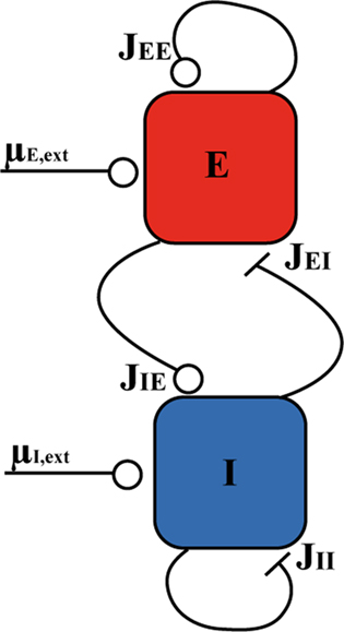
Figure 1. Schematic diagram of the network model. An open circle means that the connection is excitatory and a bar means that it is inhibitory.

2.1 Rate Models

In the simplest rate model, the instantaneous firing rates at time t, r_E,_I(t) of E and I populations, are given by (see, e.g., Wilson and Cowan, 1972; Tsodyks et al., 1997; Ermentrout, 1998; Dayan and Abbott, 2001; Murphy and Miller, 2009):

where τ_E,_I characterize the time constant of firing rate dynamics, while F_E,I(x) are the static transfer functions that describe the relationship between a mean synaptic input and an average firing rate in stationary conditions. Various types of response functions F_E,I(x) have been used in the literature. Here, in order to simplify the analysis, we take this function to be threshold-linear (see, e.g., Ben-Yishai et al., 1995; Hansel and Sompolinsky, 1998; Roxin et al., 2005)

In the simplest rate model [Eqs (1,2)], synaptic time constants are ignored. Another class of rate models assumes instantaneous firing rate dynamics, and dynamical variables are assumed to represent average synaptic currents (Ermentrout, 1998). Since synaptic time constants are known to play an important role in shaping the dynamics of the activity of neurons, we investigate a rate model in which both neuronal and synaptic time constants are present. Real synaptic currents are characterized by three qualitatively distinct time constants: a latency (interval between pre-synaptic spike and the beginning of the post-synaptic response), a rise time, and a decay time (see, e.g., Destexhe et al., 1998). The simplest way to implement such synaptic currents in a rate model is through two synaptic variables s_ab(t) and x_ab(t) (where a, b = E, I denote the post/pre-synaptic population, respectively) whose dynamics are described by the following equations

where D_ab, τ_rab, τ_sab are the latencies, rise times, and decay times of synaptic currents from population b to population a (see, e.g., Brunel and Wang, 2003). In this model, Eqs (1,2) are replaced by

where a = E, I. Note that Eqs (1,2) are recovered when D_ab = 0, τ_rab = 0, τ_sab = 0 for all a, b.

We also consider a version of the model where only the latency is described (Roxin et al., 2005). In this case, Eqs (4,5,6) are replaced by

This model corresponds to a special case of Eqs (4–6) with τ_rab = τ_sab = 0 for all a, b.

2.2 Network of Leaky Integrate-and-Fire Neurons

In this model E and I populations are composed of N_E, N_I LIF neurons (see, e.g., Tuckwell, 1988; Dayan and Abbott, 2001), with N_E + N_I = N. Each neuron i of population a is described by its membrane potential V_i(t), which obeys

where τ_ma is the membrane time constant of neurons in population a = E, I, V_rest = −70 mV is the resting membrane potential, ση_i(t) is a noise term modeling the variability in external inputs received by neurons in addition to the “signal” μ_a,ext(t), where σ is the standard deviation of the noise and η_i(t) is a white noise of unit variance, uncorrelated from neuron to neuron. Finally, s_ij(t) are individual synaptic currents from neuron j ∈ b = E, I to neuron i ∈ a = E, I, modeled as in the rate model with the help of an additional synaptic variable x_ij:

where again D_ab, τ_rab, τ_sab are the latencies, rise times, and decay times of synaptic currents from population b to population a. The sum over k represents a sum over all spikes of pre-synaptic neuron j, that occur at times Note the factor τ_ma in front of this sum, which is chosen such that (i) both x and s variables are dimensionless; (ii) the total charge of individual PSCs is independent of synaptic time constants. In this model, action potentials occur when the voltage crosses V_thr = −50 mV. At the time of the action potential, the voltage is reset at V_reset = −60 mV. For simplicity, no refractory period is included.

The instantaneous firing rate of each population r_E,I(t) is given by the sum of the number of spikes of the corresponding population in a time window dt

In numerical simulations, r_E,I(t) are computed from simulating a network of N_E = 2000 and N_I = 500 neurons, except in Figure 9 where N_E = 8000 and N_I = 2000, using a Runge–Kutta second order method with a time step dt = 0.01 ms. In the mean-field analysis, one takes the limit N → ∞, dt → 0 (see below).

2.3 External Inputs and Response of the Network

In this paper, we consider external inputs of the form

where μ_a0 is a constant external drive, and μ_a1 is the amplitude of a sinusoidal modulation in the average input at a frequency ω = 2πf.

We assume μ_a1 is sufficiently small so that the response of the network firing rate is linear in μ_a1. If this assumption is satisfied, then the firing rate response is given by

where r_a0 is a constant firing rate in absence of time-dependent modulation in the input (in other words, the background activity of the network), while r_a1(ω) describes how the instantaneous firing rate is modulated by a sinusoidal input at frequency ω. It is a complex function which describes the gain and the phase of the modulation at frequency ω. In the following, we call r_a0 the static transfer function of the network, while r_a1(ω) is the dynamical transfer function of the network. The motivation for computing the response to sinusoidal inputs is twofold: (1) one can then reconstruct the response of the network to arbitrary-time dependent inputs; (2) oscillations are observed in many regions of the central nervous system, and are therefore a common type of input for post-synaptic structures.

3 Analytical Methods

The analysis of the network response is performed in three steps. (1) we compute the background activity as a function of the mean drive (static transfer function); (2) we check whether background activity with a constant firing rate is stable; (3) we compute the dynamical response of the network. The outcome of the analysis is therefore both the region of stability of states with time-independent firing rate (i.e., asynchronous states in networks of spiking neurons) in the space of parameters characterizing the network, and the dynamical transfer function as a function of such parameters. We now briefly outline how these three steps are performed in practice.

3.1 Static Transfer Function

3.1.1 Rate models

In the rate model, with constant external inputs (μ_a1 = 0 for a = E, I), the stationary firing rates are given by

where I_a0 is the synaptic input received by population a. In this paper, we only consider the situation where both input currents are suprathreshold (I_a0 > 0 for both a = E, I).

When I_a0 > 0 for both a = E, I, we have

It is sometimes useful to rewrite both equations as follows

where X and Y measure the strength of feed-forward and feedback inhibition, respectively:

and α₀ is the ratio of the external inputs to the I population, divided by the external inputs to the E population, α₀ = μ_I0/μ_E0. Note that in this model X should be smaller than one in order for the E rate to be positive.

3.1.2 LIF network

In a network of LIF neurons, the steady-state firing rates are given by

where Φ_a(I) is given by

is the standard current-to-rate transduction function of LIF neurons in the presence of white noise (see, e.g., Siegert, 1951; Amit and Tsodyks, 1991).

3.2 Linear Stability Analysis of the Fixed Point

We use standard methods to perform the linear stability analysis of the fixed points of both rate model (see, e.g., Wilson and Cowan, 1972; Roxin et al., 2005) and network of integrate-and-fire neurons (see, e.g., Abbott and van Vreeswijk, 1993; Brunel and Hakim, 1999; Brunel, 2000; Brunel and Hansel, 2006).

The basic idea is to add a small perturbation to the steady-state firing rate,

and to compute the eigenvalues λ of the system by solving the resulting equations at first order in δr_as. Instabilities arise when at least one eigenvalue has positive real part.

In the simplest rate model [Eqs (1,2)], the eigenvalues can be computed explicitly as a solution to the following quadratic equation:

As soon as delays are included, the eigenvalues no longer have simple analytical expressions. In order to compute the eigenvalues, we use the following strategy. The first step is, for a given perturbation in the rate δr_b(t)e^λt, to compute the resulting perturbation in the average synaptic variables

where, for synaptic currents defined by Eqs (4,5),

For λ = iω, S behaves as a low-pass filter with an additional delay (see Figures 2C,D).

FIGURE 2

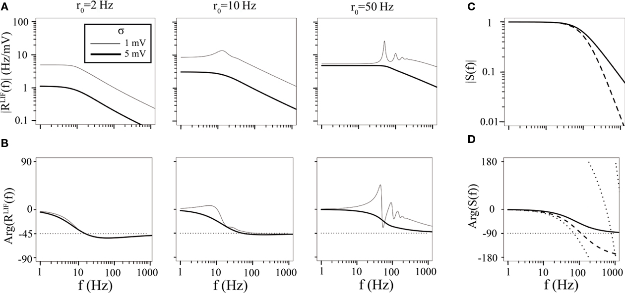
Figure 2. Neuronal (R^LIF) and synaptic (S) transfer functions. (A) Modulus (amplitude) of R^LIF as a function of frequency, for several values of the mean firing rate r₀ and the amplitude of the noise σ. R^LIF| is proportional to the slope of the static transfer function at low frequencies, and decays as at high frequency. It shows resonances at integer multiples of r₀ at high firing rates and low noise. (B) Argument (phase shift) of the R^LIF as a function of frequency, for several values of the mean firing rate r₀ and the amplitude of the noise σ. (C) Modulus of S, for τ_s = 2 ms, τ_r = 0 ms (full line) and τ_s = 2 ms, τ_r = 1 ms (dashed line). Note that the modulus is independent of the delay. It decreases at high frequency as 1/(fτ_s) when the rise time is zero, and 1/(f²τ_sτ_r) when both rise and decay times are non-zero. (D) Argument of S, for three parameter sets: D = 0 ms, τ_s = 2 ms, τ_r = 0 ms (full line); D = 0 ms, τ_s = 2 ms, τ_r = 1 ms (dashed line); and D = 1 ms, τ_s = 2 ms, τ_r = 1 ms (dotted line).

From the perturbation in the individual synaptic variables, we can easily compute the perturbation in total average currents to neurons in a population

The second step is, from a perturbation in total average currents, to compute the perturbation in the instantaneous firing rate,

where, for the rate model,

while for the network of integrate-and-fire neurons (Brunel and Hakim, 1999; Brunel et al., 2001)

where y_t = V_thr − (V_rest + I_a0)/σ, y_t = V_rest − (V_rest + I_a0)/σ, and

where M is a confluent hypergeometric function (Abramowitz and Stegun, 1970). The function R^LIF is shown in Figure 2 for λ = iω. This figure shows some of the main qualitative features of R^LIF: (i) when noise is large, it behaves as a low-pass filter, with a decay at high frequency in while resonances are present when noise is small; (ii) the gain depends markedly on both noise level, and mean firing rate.

The last step is to insert Eqs (27,29) in Eq. (30), and to divide both sides by e^λt. Eliminating δr_as, we find that the eigenvalues λ should satisfy

where

describes the net effect of the firing rate of population b on population a. Note that the three terms in the r.h.s. of Eq. (34) potentially lead to three distinct instabilities, mediated by E → E, I → I, or the E → I → E feedback loop, respectively.

Note that in the simplest rate model, S_ab(λ) = 1, R_a(λ) is given by Eq. (31), and Eq. (34) reduces to Eq. (26).

Equation (34) is solved numerically, using a globally convergent Newton routine which tracks the solutions λ = α + iβ to this equation, starting from many different initial conditions. Models are considered stable only if the routine converges toward negative αs for any initial condition.

3.3 Dynamical Transfer Function

Once linear stability of the background state has been checked, we can calculate the response of the system when the input has an additional oscillatory component. The oscillatory response of population firing rates is given by

where in the above equations A_ab is given by Eq. (35) in which λ = iω, and R_a is given by Eq. (31) for the rate models, Eq. (32) for the network of integrate-and-fire neurons, in which λ = iω.

4 Results

4.1 One-Population Model

It is useful to start by summarizing the dynamics of a network of a single population of neurons, before moving to the two-population network. In a rate model, the stationary firing rate r₀ is given by

where μ₀ is the external input, and J is the recurrent coupling (excitatory if J > 0, inhibitory if J < 0). In a network of LIF neurons, the stationary firing rate r₀ is given by

Linear stability analysis of the system shows that the eigenvalues λ satisfy

where R(λ) is given by Eq. (31/32) for rate model/network of LIF neurons, respectively, and S(λ) = 1 for the simplest rate model, and is otherwise given by Eq. (28).

When the asynchronous state is stable, the dynamical transfer function is

In the absence of coupling, the network firing rate behaves as a low-pass filter (see the gray curves in Figure 3), except in the LIF network in the small noise regime where resonances appear at the single neuron firing frequency (see, e.g., Knight, 1972; Brunel et al., 2001; Fourcaud and Brunel, 2002; Fourcaud-Trocmé et al., 2003 and Figure 2 – regime not shown in Figure 3).

FIGURE 3

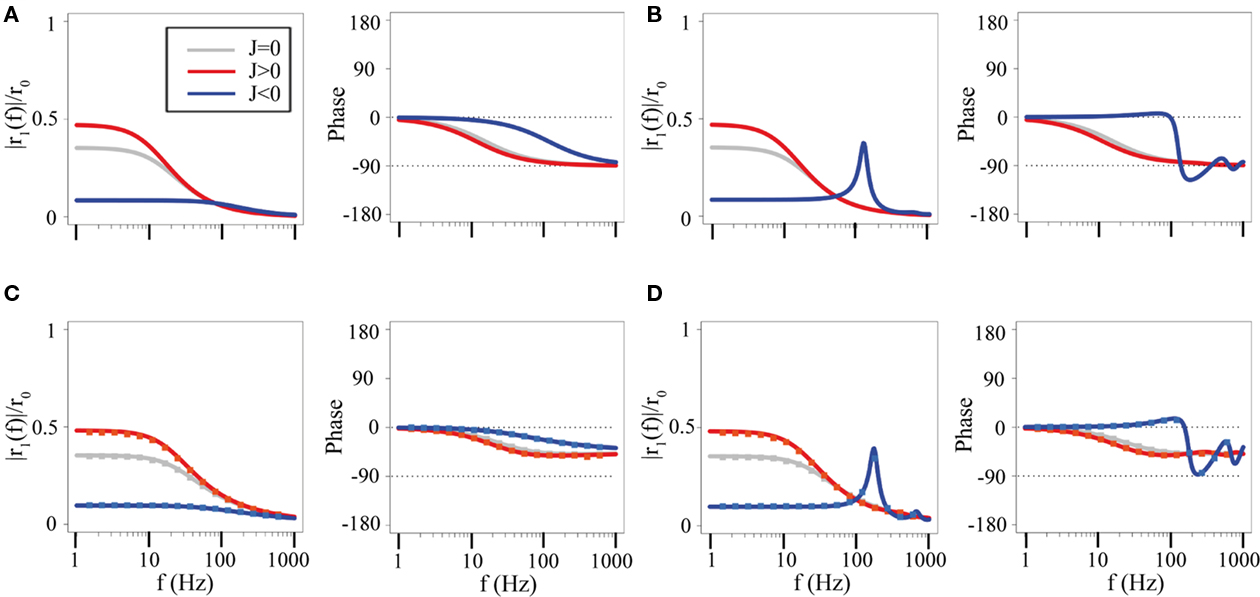
Figure 3. Dynamics of one-population networks. Amplitude and phase shift of the network rate response to an oscillatory input at frequency f. (A) Rate model with no delays, τ = 10 ms. Gray line: unconnected network (J = 0). Red line: excitatory network (J = 0.25). Blue line: inhibitory network (J = −6.5). (B) Rate model with a delay, D = 2 ms. Otherwise same parameters as in (A). (C) Network of LIF neurons (τ_m = 10 ms, r₀ = 15 Hz, σ = 5 mV) with no delay. Lines: analytical expression, Eq. (39); Squares: numerical simulations of a network of 2000 neurons. As in A, gray: unconnected network (J = 0 mV); Red: excitatory network (J = 5 mV); Blue: inhibitory network (J = −50 mV). (D) Network of LIF neurons with delay D = 2 ms. Other parameters as in (C).

In an excitatory network (J > 0), the asynchronous state is stable provided J < J_c where J_c = 1 (rate model), J_c = 1/Φ′(Φ⁻¹(r₀)) (LIF network). When J = J_c, one of the eigenvalues becomes equal to zero, signaling the onset of a saddle-node bifurcation. This is the much-studied rate instability: because of the excitatory feedback, the network cannot maintain its rate at a value r₀. Rather, the rate either decreases to a smaller value (typically close to zero), or increases to a larger value (typically close to maximal firing rate). When J < J_c, the effect of excitatory coupling is to amplify the response at low frequencies (the much-studied amplification effect, see Figure 3, red curves, and Seung, 2003), while at the same time slowing down the dynamics (through a reduction of the cut-off frequency, see, e.g., Seung, 2003). This effect is present in all models, independently of synaptic characteristics.

In the simplest inhibitory network (no synaptic time constants), the asynchronous state is always stable. Introducing a delay in synaptic transmission leads to an oscillatory instability (through a Hopf bifurcation) at a frequency ω. In the rate model in which no rise and decay times are present, the frequency ω satisfies the equation tan(ωD) = −τω, whose solution is ω ∼ π/2D when D ≪ τ (Roxin et al., 2005; Brunel and Hakim, 2008). This instability leads to an oscillation due to delayed inhibitory feedback when |J| > |J_c|, which has been characterized in many different inhibitory network models (see Brunel and Hakim, 2008 for a review). When |J| < |J_c|, the effect of inhibitory coupling is to suppress the response at low frequencies, which leads to an increase in the cut-off frequency (see, e.g., Seung, 2003). In the absence of delays, the response of the network is basically the response of a low-pass filter. In the presence of a delay, the response shows a resonance at a frequency close to the frequency of the oscillation at the Hopf bifurcation (see Figures 3B,D, blue curves).

4.2 Two-Population Rate Models

4.2.1 Stability of the asynchronous state in the simplest rate model

In the simplest rate model, the eigenvalues of the linear stability matrix are given by Eq. (26). From this equation it is easy to compute the conditions the coupling parameters must satisfy on the two possible types of instability lines.

A saddle-node bifurcation occurs when λ = 0; this happens whenever

or equivalently 1 + Y = 0. This instability corresponds to the rate instability induced by excitatory feedback onto the excitatory population, which is already present in the one-population model. The presence of feedback inhibition (as measured by the parameter Y) stabilizes the network with respect to this instability.

A Hopf bifurcation occurs when λ = iω this happens whenever

This bifurcation is a new feature of the two-population model; it depends both on E–E feedback and the E–I feedback loop. The two bifurcation lines are shown in Figure 4.

FIGURE 4

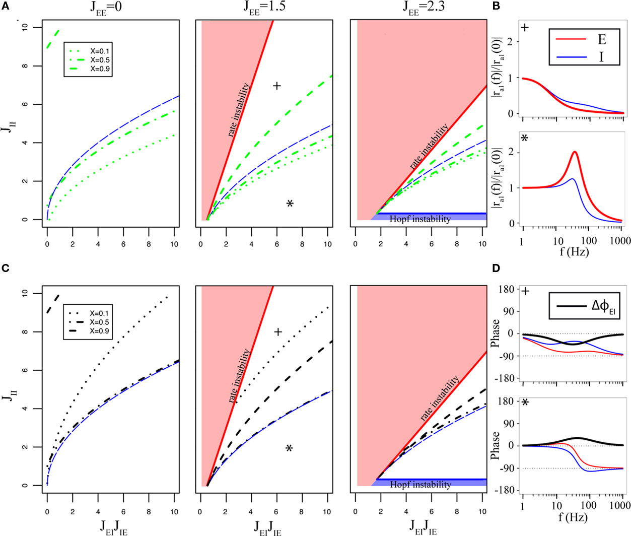
Figure 4. Qualitative behaviors of the network transfer function in the simplest two-population rate model. (A) Behaviors of the amplitude of the E network in the J_EIJ_IE − J_II plane, for three different values of J_EE (indicated at the top of the corresponding panels). Red/blue areas show regions in which the asynchronous state is unstable due to the rate/Hopf instability, respectively. Above the dashed blue line, eigenvalues are real; below the line, they have a non-zero imaginary part. Green dashed/dotted lines indicate the boundary of the region in which the transfer function is of the low-pass type (above the lines) or resonant (below the lines), for different values of X (indicated on left panel). (B) Amplitude vs frequency curves, for two representative examples [+: J_EE = 1.5, J_EIJ_IE = 6, J_II = 7, X = 0.5, *: J_EE = 1.5, J_EIJ_IE = 7, J_II = 1, X = 0.5, both indicated by the corresponding symbols in the middle panel of (A)]. Both panels show the amplitude of the modulation of the E (red) and I (blue) populations. (C) Behaviors of the phase shift between E and I populations. Same conventions as in A except that black dashed/dotted lines indicate the boundary of the region in which the I population leads the E population at all frequencies (above the lines), or the opposite (below the lines), again for different values of X (indicated on left panel). (D) Phase vs frequency curves for two representative examples [+: J_EE = 1.5, J_EIJ_IE = 6, J_II = 8, X = 0.5. *: J_EE = 1.5, J_EIJ_IE = 8, J_II = 2, X = 0.5, again indicated by the corresponding symbols in the middle panel of (C)]. Both panels show the phase shift of the E (red) and I (blue) populations with respect to the input, as well as the phase shift between E and I populations (black). In all cases, τ_E = τ_I = 10 ms.

4.2.2 Dynamical transfer function in the simplest rate model

For a two-population rate model, the dynamical transfer function is given by Eqs (36,37), which can be rewritten for the simplest rate model as

Where is the effective time constant of the population a,

In writing Eqs (40,41), we have assumed that α₁ ≡ μ_I1/μ_E1 is equal to α₀ = μ_I0/μ_E0. This would be the case if both E and I networks receive inputs from the same structures. If E and I networks receive different types of inputs, then we could in principle have α₁ ≠ α₀. In this case, we would need to define two effective feed-forward parameters X₀ (strength of “static” feed-forward inhibition) and X₁ (strength of “dynamic” feed-forward inhibition), proportional to α₀ and α₁, respectively.

We focus here on two quantities: the amplitude of the excitatory transfer function |r_EI(ω)|, and the phase shift between the two-populations, ΔΦ_EI(ω). In this model, it is easy to show (see Appendix) that the amplitude of the transfer function can have only two qualitatively different behaviors: (i) a monotonically decaying function of the frequency ω (“low-pass” behavior – see, e.g., Figure 4B, panel with the cross); or (ii) a function that first increases with frequency, peaks at a finite frequency, and then decays toward zero at high frequencies (see Figure 4B, panel with the star). Note that in the rate model the amplitude of the response does not depend on r_a0. Therefore the examples in the Figures 4, 5, and 6 are shown with amplitudes normalized by r_a1(f = 0) and not r_a0. The regions where both types of behaviors occur are shown in the plane of couplings involving the inhibitory network (self-inhibitory coupling J_II vs strength of EI loop J_EIJ_IE), for different values of J_EE, in Figure 4A. We see that strong values of J_II tend to favor low-pass behavior, while strong values of J_EIJ_IE tend to favor resonant behavior. Close to the saddle-node bifurcation, the transfer function is low-pass, with a zero-frequency response that diverges on the bifurcation line. Close to the Hopf bifurcation, the transfer function is resonant, with a peak that diverges on the bifurcation line, at the frequency of the oscillation that appears on the line.

FIGURE 5

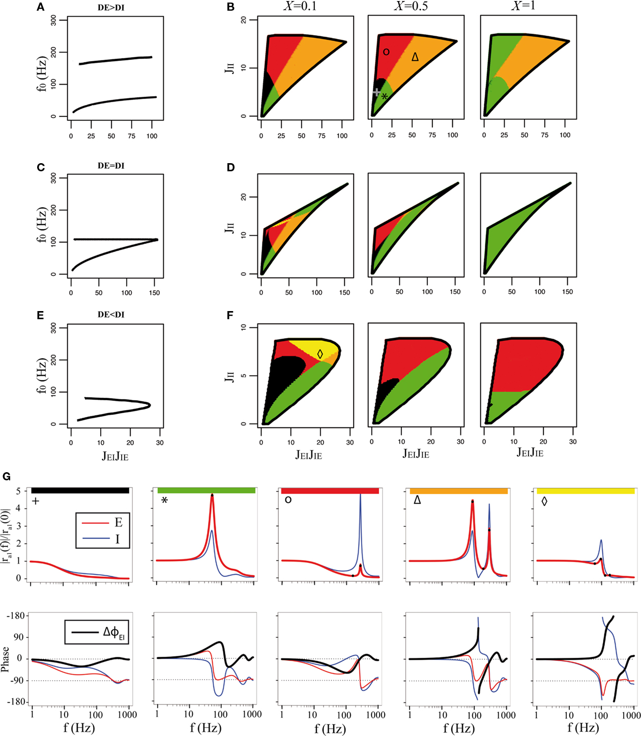
Figure 5. Qualitative behaviors of the rate model with delays, for τE = τI = 10 ms, JEE = 1. 5. (A,B) D_E = 2 ms, D_I = 1 ms, (C,D) D_E = D_I = 1.5 ms; (E,F) D_E = 1 ms, D_I = 2 ms. (A,C,E) frequency of the oscillatory instability on the bifurcation lines, as a function of J_EIJ_IE. (B,D,F) behaviors of the gain of the E network in the J_EIJ_IE − J_II plane for three different values of X (indicated at the top of the corresponding panels). White areas show regions in which the asynchronous state is unstable due to the rate or Hopf instabilities, shown as black lines. The stable region is subdivided in regions of different colors, indicating qualitatively different behaviors of the E transfer function. Colors indicate the number of extrema at non-zero frequencies of the amplitude vs frequency curve (0: black, 1: green, 2: red, 3: orange, 4: yellow). (G) Representative transfer functions (top: amplitude; bottom: phase) for each of the regions. From left to right, J_EIJ_IE = 5, 18, 23, 80, 19; J_II = 5, 4, 15.5, 14, 7. Symbols on the top left of the amplitude plots refer to the location of the network parameters in (B,F). Black dots on top of the red curves indicate the location of the extrema.

FIGURE 6

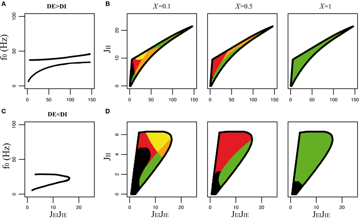
Figure 6. Qualitative behaviors of the rate model with non-zero delays, rise, and decay times (τsEE = τsEI = 2 ms, τsIE = τsII = 5 ms, and τrEE = τrEI = τrIE = τsII = 1 ms). Other parameters: τ_E = 20 ms, τ_I = 10 ms, J_EE = 1.5. (A) Frequency of the oscillatory instabilities as a function of J_EIJ_IE for D_E = 2 ms, D_I = 1 ms. (B) Stability region of the asynchronous state in the J_EIJ_IE − J_II plane, and qualitative behaviors of the E transfer function for D_E = 2 ms, D_I = 1 ms, and three values of X (same color codes as in Figure 5). (C) Frequency of the oscillatory instability for D_E = 1 ms, D_I = 2 ms. (D) Stability region of the asynchronous state, and qualitative behaviors of the E transfer function for D_E = 1 ms, D_I = 2 ms, and three values of X (same color codes as in Figure 5).

The boundary separating the two regions depends on the strength of feed-forward inhibition X: the larger X, the more pronounced the resonant behavior. This is because feed-forward inhibition tends to suppress inputs at low frequencies. In fact, feed-forward inhibition can create a resonance even in the absence of feedback E–I coupling (see Figure 4A, case where J_EE = 0). In the limit X → 1, the resonant behavior becomes present in the whole stable region. Note also that the presence of a resonance is not equivalent to the presence of complex eigenvalues of the linear stability analysis, as happens in a two-variable single neuron model (Richardson et al., 2003): the network can be resonant in the absence of complex eigenvalues, and conversely, the network can be low-pass in the presence of such complex eigenvalues.

Another quantity of interest is the phase shift between excitatory and inhibitory populations. In this model, one can show (see Appendix for details) that again only two qualitatively different behaviors can occur: (i) the excitatory population leads the inhibitory population at all frequencies f (see, e.g., Figure 4D, panel with the cross); or (ii) the opposite occurs and the inhibitory population leads the excitatory population at all f (see, e.g., Figure 4D, panel with the star). The regions where both types of behavior occur are shown in the plane of couplings involving the inhibitory network (self-inhibitory coupling J_II vs strength of EI loop J_EIJ_IE), for different values of J_EE, in Figure 4C. Close to the rate instability, inhibition tends to lead excitation, while the opposite occurs close to the Hopf bifurcation. Note that for all parameters, the phase shift between the two-populations tends to zero in both f → 0 and f → ∞ limits, and that it reaches a maximum at some finite value. In the resonant region, this value is close to the location of the resonant peak (compare Figures 4B,D, panels with the star).

4.3 Rate Model with Non-Zero Synaptic Time Constants

How are the dynamics modified when the synaptic time scales are taken into account in the rate model? We show here that new behaviors emerge, due to the presence of delays in synaptic interactions.

4.3.1 Stability of the asynchronous state

The stability of the asynchronous state can be evaluated by computing the eigenvalues, i.e., the solutions of Eqs (34,35,28,31). We first discuss the stability analysis when synaptic interactions are simply described by a delay (i.e., rise and decay times are equal to zero), and both E and I populations have the same rate time constant. In fact, all the qualitative features of the general case (i.e., with strictly positive rise times and decay times, and/or with τ_E ≠ τ_I) are already present in this simplified model.

The main qualitative changes that occur when delays are introduced are as follows: (1) there is a new oscillatory instability induced by I–I connectivity, which is reached when J_II becomes strong enough (Brunel and Hakim, 1999; Roxin et al., 2005); (2) the oscillatory instability induced by the E–I feedback loop is now present at all values of J_EE. As a result of the new oscillatory instability, the space of parameters for which the asynchronous state is stable is now bounded for any value of J_EE (see Figure 5). The number of distinct bifurcation lines that form the boundary of the region of stability can vary between one and three, depending on parameters. First, the rate instability line is only present when J_EE > 1, as in the simplest rate model without synaptic time constant. Second, there can be either one or two distinct oscillatory instability lines, depending on the relative values of the excitatory and inhibitory delays, D_E and D_I.

When D_E > D_I, there exist two distinct instability lines, characterizing the I–I and E–I scenarios; these two lines cross at some point in the J_II − J_EIJ_IE plane (see Figures 5A,B). The frequencies of the corresponding instabilities remain well separated. The frequency of the I–I instability is generically higher than the frequency of the E–I instability, since the I–I induced-oscillations involve only two synapses from peak to peak (increase in I rate leads to a decrease in I rate due to I feedback, which in turn leads to the next increase in I rate), while E–I induced-oscillations involve four synapses (E rate increases, leading to an increase in I rate, leading to a decrease in E rate, then decrease in I rate, followed by the next increase in E rate). For example, for the parameters of Figure 5A, I–I instability leads to frequencies in the 150 to 200-Hz range, while E–I instability leads to frequencies which are in the 10 to 80-Hz frequency range. When D_E = D_I, the two instability lines meet at a cusp; at this point the frequencies of the two instabilities become equal (Figure 5C). Finally, when D_E < D_I there is a single oscillatory instability line, smoothly connecting the “pure” I–I and “pure” E–I scenarios in the J_II − J_EIJ_IE plane (Figure 5F). In this case the frequency decreases smoothly along the line as the J_II/J_EIJ_IE ratio is decreased. As a result, the region of stability of the asynchronous state exhibits either a triangular shape, when D_E ≥ D_I (see Figures 5B,F) or a D shape, when D_E < D_I (see Figure 5F).

4.3.2 Dynamical transfer function

The next step is to compute the dynamical transfer function, Eqs (36,37). We show in Figure 5 how the qualitative shape of this transfer function depends synaptic parameters and on the connectivity strengths. In the vicinity of the rate instability, the transfer function has either low-pass characteristics (black regions in Figure 5, see a representative transfer function in Figure 5G), or shows a trough followed by a resonant peak, when the system is close to the I–I instability (red region in Figure 5, see a representative transfer function in Figure 5G). In the vicinity of the Hopf bifurcation lines, the transfer function always exhibits resonant peaks, but in qualitatively different ways. There can be a single resonant peak – the typical situation when the stability region is D-shaped, i.e., there is a single bifurcation line (see green, red, and yellow regions in Figure 5, and the corresponding transfer functions in Figure 5G). Note that in the yellow region, there is a second peak in the transfer function at a frequency which is larger than the one of the resonant peak, but its magnitude is always small compared to the amplitude of the other peak. Alternatively, there can be two separate resonant peaks, typically when the stability region is triangular, i.e., with two separate bifurcation lines, with two separate frequencies (see orange regions in Figure 5B, and the transfer function in Figure 5G), and the network is close to the intersection between the two lines. The frequency of the resonant peaks is close to the frequency of the corresponding instabilities. For parameters of Figure 5, the resonant frequency is typically in the gamma range when the system is close to the E–I bifurcation line, while it is typically very high (more than 100 Hz) when the system is close to the I–I line. As in the simplest rate model, the boundary between the different regions also depends on the strength of feed-forward inhibition: in particular, the pure low-pass region tends to disappear as X increases, since a high value of X decreases the response at low frequencies.

The transfer functions can also be classified according to the behavior of the phase shift between excitatory and inhibitory populations. The main new behavior introduced by the presence of synaptic delays is that it is now possible for the phase shift to change sign when the frequency is increased. This leads to a larger number of qualitatively different behaviors for the phase shift. Some of the typical behaviors of the phase shift are represented in Figure 5G. Note in particular that resonances are associated with sharp changes in the phase shift. Close to the E–I instability line, the E population leads the I population at the corresponding resonant frequency.

The behavior of a model with τ_E ≠ τ_I is qualitatively very similar to the one of the model with τ_E = τ_I. The main difference is that the transition between the 1 Hopf and 2 Hopf bifurcation behaviors no longer occurs at D_E = D_I, but for slightly different values of the delays. For example, for τ_E = 20 ms, τ_I = 10 ms, and D_E = 1.5 ms, the transition between both behaviors occurs at D_I ∼ 1.55 ms.

4.3.3 Behavior of the model with finite rise and decay times

A similar analysis can be performed for the rate model with finite delay, rise, and decay times. The qualitative behaviors of the transfer function in the region of stability of the asynchronous state are shown in Figure 6. This figure shows that the same types of behaviors are observed as in Figure 5. At the quantitative level, the frequencies of the instabilities are reduced by the presence of finite rise/decay times (compare Figures 6A,C with Figures 5A,E). This decrease in frequency is stronger for the I–I instability. Consequently, the two possible resonant frequencies are now much closer than in the case in which only delays are present, which decreases the size of the region in which both resonances are observed (compare orange regions in Figures 5 and 6). Another quantitative difference is that phase differences between E and I populations tend to be smaller.

4.4 Network of LIF Neurons

The same analysis can be performed for a network of LIF neurons, as outlined in Section 3.2. Interestingly, the stability analysis of the asynchronous state revealed the same types of instabilities as in the rate model with synaptic time constants, i.e., a rate instability (mostly governed by E–E interactions), and two types of oscillatory instabilities (governed by E–I or I–I interactions). As in the rate model, the two types of oscillatory instabilities merge smoothly in the space of synaptic connection strengths if D_E < D_I, while they remain disjoint if D_E = D_I. There are however a few qualitative differences between the two models:

• The high frequency behavior of the LIF model is different from the rate model: the amplitude of the response decays as , and the phase shifts go to π/4, in the LIF network, as compared to a 1/f decay with a phase shift of π/2 in the rate model (see Section 5)

• In the LIF network, the single neuron transfer function depends both on its average inputs (and therefore its average firing rate) and on the level of noise. As a consequence, the network transfer function changes as a function of both mean and variance of the external inputs.

In this section we first show how the qualitative behaviors of the LIF network compare with those of the rate model (at fixed mean firing rate and level of noise), and then show how external inputs can qualitatively change the network transfer function in the LIF network. This property is not present in a rate model with threshold-linear static transfer function, but can be reproduced with a suitable non-linearity in the static transfer function.

4.4.1 Comparison between LIF network and rate model

Figure 7 shows the behaviors of the transfer function of the LIF network in strong noise regime (σ = 5 mV). To make an explicit comparison with the rate model, we choose to fix the firing rates of E and I populations to specific values (10 Hz and 30 Hz, respectively), independently of the matrix of coupling. This means that on any point of the phase diagrams showed in Figure 7 the external inputs must be computed such that the network has the required mean firing rates. We also need to generalize the definition of the feed-forward and feedback inhibition parameters to the LIF network. A natural generalization is

FIGURE 7

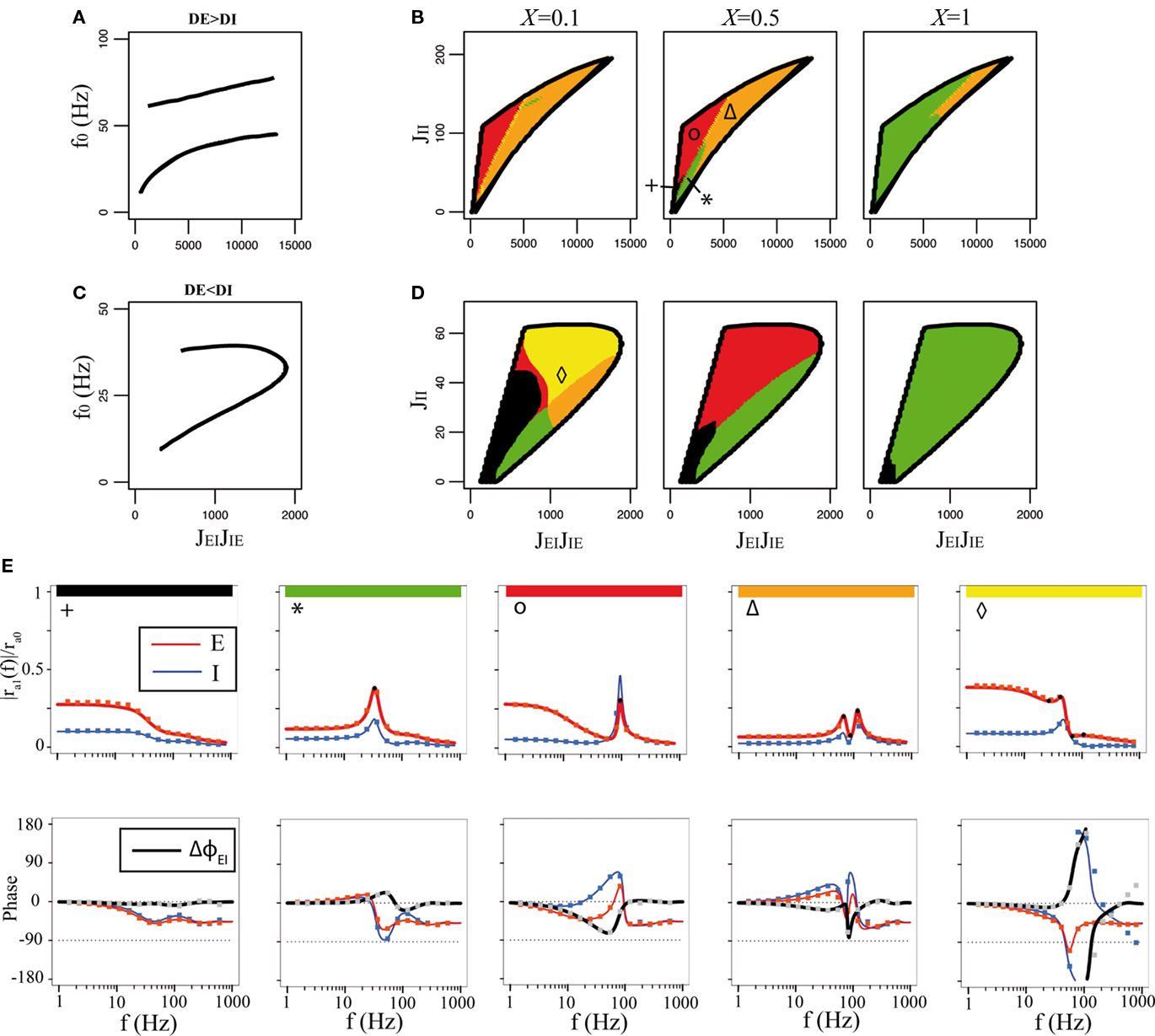
Figure 7. Qualitative behaviors of the network of LIF neurons. Synaptic time constants are the same as in Figure 6. Color codes as in Figure 5. In all cases, r_E0 = 10 Hz, r_I0 = 30 Hz and μ_E1 = 1 mV, τ_mE = 20 ms, τ_mI = 10 ms, J_EE = 25 mV. (A) Frequency of the oscillatory instabilities for D_E = 2 ms, D_I = 1 ms. (B) Stability region of the asynchronous state, and qualitative behaviors of the E transfer function for D_E = 2 ms, D_I = 1 ms, and three values of X. (C) Frequency of the oscillatory instability for D_E = 1 ms, D_I = 2 ms. (D) Stability region of the asynchronous state, and qualitative behaviors of the E transfer function for D_E = 1 ms, D_I = 2 ms, and three values of X. (E) Representative transfer functions of each behavior. Lines: analytical expressions, Eqs (36,37). Squares: numerical simulations of a network of 2000 excitatory neurons and 500 inhibitory neurons. From left to right: J_EIJ_IE = 600, 1300, 2000, 8000, 1100 mV and J_II = 20, 30, 100, 150, 40 mV.

In Eqs (42,43), we see that these parameters are now governed by “effective coupling strengths,” where the coupling strength J_ab is multiplied by the gain of the transfer function of the pre-synaptic population at the corresponding firing rate.

To compare the LIF network with the rate model, we then modulated independently the sinusoidal inputs to the E and I populations, but with a ratio between amplitudes taken in order to keep the feed-forward inhibition parameter X constant in each plot. Synaptic parameters was taken to be identical to the rate model. Figure 7 shows that, qualitatively, the LIF network behaves essentially as the rate model. There are of course quantitative differences due to the fact the transfer function of the LIF neuron is different from that of the rate model. Importantly, the high frequency behavior is different, with a decay of the gain, and a phase shift of 45° at high frequencies in the LIF model, as already mentioned above.

4.4.2 Dependence of the network transfer function on external inputs

In the LIF model, the single-cell transfer function R^LIF depends on the inputs to the network. In particular, changing the overall firing rate alters the static gain of the transfer function Φ, which changes the effective coupling strengths and in turn the effective feed-forward and feedback inhibition parameters.

Figure 8 shows an example of a network where an increased input to both populations led to qualitative changes of the network transfer function. The coupling strengths were chosen such that when the external inputs to both populations increase, the firing rates of both populations first increase. Then, inhibition becomes strong enough to reduce excitatory rates even with the increased external inputs. Interestingly, this leads to a feed-forward parameter X larger than one. The network transfer function goes through a number of changes as the external inputs are varied: at low input strength/low rates, the transfer function is low-pass, due to the fact that the gain of single neuron f–I curves is small, and hence effective coupling strengths are small. When the inputs increase, the slopes of the transfer functions increase, and therefore the effective couplings increase. This leads to a resonant transfer function, due to feedback between E and I populations. Finally, when the inputs increase further, the E rate reaches a peak and then decreases with increased inputs. This leads to a major change of the response to external inputs: the E and I populations are now in antiphase for slowly varying inputs (see Figure 8D). This is due to the fact that X > 1. When X = 1, then the phase shift between the two-populations is 90°, as shown by Figure 8D. In both cases, the phase shift between the two-populations decreases with frequency, and goes to zero in the high frequency limit.

FIGURE 8

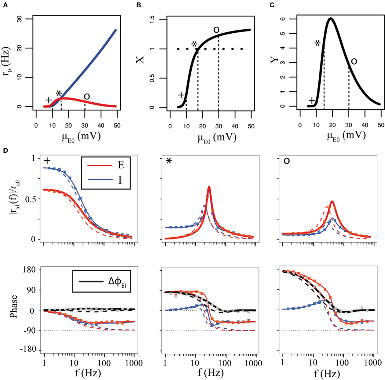
Figure 8. External inputs can change qualitatively the network transfer function. Parameters of the network are μ_E1 = 1 mV, τ_mE = 20 ms, τ_mI = 10 ms, synaptic time constants as in Figure 6B, J_EE = 25 mV, J_EIJ_IE = 6400 mV, J_II = 70 mV. (A) Firing rate of E (red) and I (blue) populations as a function of external input. (B) Feed-forward inhibition parameter X as a function of μ_E0. (C) Feedback inhibition parameter Y as a function of μ_E0. (D) Network transfer functions for three different values of μ_E0, indicated by the corresponding symbols in (A–C). From left to right panel, μ_E0 = 10, 17.4, 30 mV, corresponding to X = 0.2, 1, 1.2, r_E0 = 0.9, 2.8, 1.7 Hz and r_I0 = 0.3, 4.3, 12.3 Hz. Solid lines: analytical expressions for the LIF network, Eqs (36,37). Squares: numerical simulations of the LIF network. Dashed lines : analytical expressions for a rate model with a LIF static transfer function.

A qualitative change in network transfer function with increasing external input is a feature that is not present in a rate model with threshold-linear static transfer function, but it can be obtained using a suitable non-linear transfer function. In particular, Figure 8D shows when one uses a rate model with the static transfer function of the LIF neuron, Eq. (24), one obtains network transfer functions which are very similar to the LIF network.

4.4.3 Dependence of the network transfer function on external noise

The single-cell transfer function also depends on the magnitude of external noise, as shown by Figure 2. In particular, as was characterized in a number of previous studies (Knight, 1972; Brunel et al., 2001; Fourcaud and Brunel, 2002; Fourcaud-Trocmé et al., 2003), the single-cell transfer function exhibits pronounced resonances at integer multiples of the single-cell firing rate at low noise, while these resonances disappear at high noise and the transfer function becomes low-pass.

This qualitative change in the single-cell transfer function affects the network behavior, as seen in Figure 9, which shows the qualitative behaviors of the network transfer function as a function of a parameter g measuring the ratio between inhibitory and excitatory connection strengths (i.e., we choose J_II = J_EI = gJ_EE = gJ_IE), and the strength of external inputs. Parameters are chosen such that the network can potentially have a double resonance, due to E–I feedback coupling and I–I coupling, respectively (the orange region on the plots). The top graphs show the “phase diagram” in the high noise regime (σ = 5 mV) that has been explored so far. We see that the asynchronous state is stable in a finite range of external inputs. As the external inputs increase, the network transfer function develops a single or several resonances, depending on the value of g. Above a critical value of the external inputs the asynchronous state destabilizes due to a Hopf bifurcation, as in Brunel (2000).

FIGURE 9

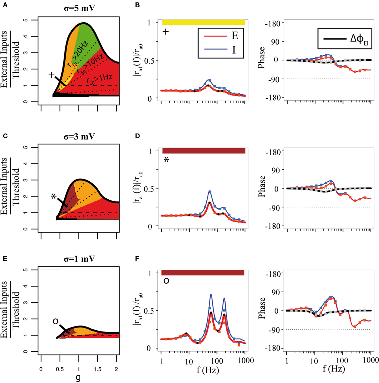
Figure 9. Network transfer functions of LIF model depend on external noise. (A) Qualitative behaviors of the E transfer function in the g − μ_E,0/(V_thr − V_rest) plane for σ = 5 mV. Same color codes as in the Figure 7, with a new region (with five extrema – three maxima and two minima, in brown). Dotted lines are iso-excitatory firing rate lines. Dashed line indicates where the input current is equal to the firing threshold. (B) Representative transfer function in the yellow region [see + sign in (A)]. Full lines: analytical expressions, Eqs (36,37). Squares: numerical simulations of a network of 8000 excitatory neurons and 2000 inhibitory neurons. (C) Same as A, but with σ = 3 mV. (D) Representative transfer function in the brown region in (C). (E) Same as A, but with σ = 1 mV. (F) Representative transfer function in the brown region in E. In all cases, α = 1, μ_E1 = 1 mV (except case F where μ_E1 = 0.5 mV), J_EE = 75 mV. Same time constants as in Figure 6. For (B,D,F) respectively: σ = 5, 3, 1 mV, r_E0 = 11.4, 8.8, 5.9 Hz and r_I0 = 22.8, 17.7, 11.8 Hz.

The other two graphs show how the picture is modified when the level of external noise decreases. There are two main effects: first, the region of stability of the asynchronous state becomes smaller, as expected from previous studies in purely inhibitory networks (Brunel and Hakim, 1999; Brunel and Hansel, 2006); second, qualitatively new behaviors of the network transfer function emerge. In particular, the network can develop a new resonance which is associated with the single-cell resonance (see Figures 9D,F).

5 Discussion

In this paper, we have investigated how the transfer function of an E–I network is controlled by its connectivity and the temporal parameters of its synapses. We have shown that a two-population rate model, as well as a fully connected network of excitatory and inhibitory integrate-and-fire neurons, exhibit many qualitatively different behaviors, from low-pass to multiple resonances. Resonance phenomena appear generically in both models provided inhibition is sufficiently strong. With realistic synaptic currents, oscillatory instabilities can arise due both to the E–I feedback loop and to the I–I connectivity. Close to these instabilities, a single or double resonance can appear, depending on synaptic parameters. We have also shown that for a given level of external input, and in a high noise regime, the behaviors of the network transfer function of LIF networks is qualitatively similar to the rate models with identical synaptic dynamics. However, an important difference is that in the network of LIF neurons the transfer function depends on the level of external inputs, and external noise. In a rate model with a threshold-linear transfer function, the “single-cell” dynamical transfer function is independent of the input. If a sigmoidal static transfer function had been used instead of the threshold-linear one, then the gain at zero-frequency (i.e., the slope of the f–I curve) would depend on the input, which could also lead to qualitative changes of the network transfer function as a function of the input. However, the LIF neuron has the additional feature that the single-cell dynamical transfer function can exhibit qualitative changes as a function of its inputs, such as the appearance of a resonance at single-cell firing frequency when the noise is sufficiently weak.

There is an extensive literature describing the bifurcations of fixed points in firing rate/neural field/neural mass models (see, e.g., Wilson and Cowan, 1972; Borisyuk and Kirillov, 1992; Jansen and Rit, 1995; Roxin et al., 2005; Deco et al., 2008; Spiegler et al., 2010) and of asynchronous states in networks of LIF neurons (see, e.g., Abbott and van Vreeswijk, 1993; Brunel and Hakim, 1999; Brunel, 2000; Hansel and Mato, 2003; Brunel and Hansel, 2006), which has already characterized at length the bifurcations that have been described here. On the other hand, only a few studies have investigated systematically how networks respond to dynamical inputs. Tsodyks et al. (1997) and Murphy and Miller (2009) in particular investigated the dynamics of a rate model in the “inhibition-stabilized” regime, i.e., J_EE > 1 in the rate model. Our analysis is also closely related to finite-size dynamics of networks of integrate-and-fire neurons in the presence of constant external inputs (Brunel and Hakim, 1999; Brunel, 2000; Mattia and Del Giudice, 2002, 2004; Kriener et al., 2008). Dynamics of stochastic versions of rate models have also been recently studied in detail (Bressloff, 2009; Buice et al., 2010). Transfer functions of networks of IF neurons with a specific architecture have also been derived previously in Doiron et al. (2004) and Lindner et al. (2005), where it was shown that global oscillations depend on the correlations in inputs. Transfer functions of gap-junction coupled networks have been studied by Ostojic et al. (2009) and Dugue et al. (2009), where it was shown that gap-junction coupling enhances resonances at the firing frequency of single-cells. The functional consequences of feed-forward inhibition for information transmission have also been studied in a number of recent studies (e.g., Akam and Kullmann, 2010; Kremkow et al., 2010a,b). The present paper is to our knowledge the first detailed comparative study of network transfer functions of both rate models and synaptically coupled networks of LIF neurons.

Input-dependent changes in the network transfer function could underlie several prominent phenomena observed in vivo in different areas. In visual cortex, the power spectrum of the LFP typically decays monotonically at low contrast, while a plateau or even a peak in the gamma frequency emerges at high contrast (Henrie and Shapley, 2005). Input-dependent changes of the transfer function at gamma frequency (due to the emergence of a resonance) has been modeled in a framework similar to ours by Kang et al. (2010). Such input-dependent changes could underlie the high information content of the gamma range in the LFP (Belitski et al., 2008), as shown by Mazzoni et al. (2008). It could also underlie the phenomenon of cross-frequency coupling, through which the power of a fast oscillation is strongly modulated by the phase of a slower oscillation, as is the case in the hippocampus (Bragin et al., 1995) as well as in primary sensory cortices (Whittingstall and Logothetis, 2009; Mazzoni et al., 2010).

This study could be generalized in a number of ways. First, it could be generalized to more realistic single-cell models such as the exponential integrate-and-fire (EIF) neuron (Fourcaud-Trocmé et al., 2003), since an efficient method has been introduced to compute both the static and dynamic single-cell transfer function for this model (Richardson, 2007). Interestingly, the transfer function of the EIF model has a high frequency behavior which is qualitatively identical to the rate model (a 1/f decay at high frequency, associated with a phase shift of 90°). This led Ostojic and Brunel (2011) to propose a reduction of the EIF model to an (adaptive) rate model, whose parameters (time constant and static transfer function) can be computed analytically from the parameters of the underlying EIF model. From these results, we expect the dynamics of networks of EIF neurons to be even closer to rate models, compared to LIF networks, provided of course the noise is sufficiently strong.

A second generalization would be to study networks of more than two-populations. It would be of interest, for example, to understand how the presence of functionally different classes of interneurons affect network dynamics. Finally, it would also be of interest to study the transfer function of randomly connected networks (Brunel and Hakim, 1999; Brunel, 2000), or of networks with more structured connectivity (Ben-Yishai et al., 1995; Roxin et al., 2005).

In this paper, we have computed how the population firing rate reacts to time-dependent inputs. Experimentally, the firing rate of small populations of neurons can be observed through MUA. Another experimental observable is the LFP. In cortex and hippocampus, the LFP is assumed to be related to the average synaptic inputs received by pyramidal cells of the main network. Given a model of how the LFP depends on synaptic currents (e.g., Mazzoni et al., 2008), one could compute the dynamics of the LFP signal using the methods used in this paper.

Finally, this work offers insight into the relationship between network connectivity and experimental observables such as phase shifts of different populations in the network. It could be used to predict network connectivity from observed patterns of resonances and phase shifts, in areas where this information is available.

Conflict of Interest Statement

The authors declare that the research was conducted in the absence of any commercial or financial relationships that could be construed as a potential conflict of interest.

Acknowledgments

We thank Boris Barbour and Vincent Hakim for useful discussions at the initial stage of the project, and for a critical reading of the manuscript. We also thank David Hansel for useful suggestions.

References

Abbott, L. F., and van Vreeswijk, C. (1993). Asynchronous states in a network of pulse-coupled oscillators. Phys. Rev. E 48, 1483–1490.

Abramowitz, M., and Stegun, I. A. (1970). Tables of Mathematical Functions. New York: Dover Publications.

Akam, T., and Kullmann, D. M. (2010). Oscillations and filtering networks support flexible routing of information. Neuron 67, 308–320.

Pubmed Abstract | Pubmed Full Text | CrossRef Full Text

Amit, D. J., and Brunel, N. (1997). Model of global spontaneous activity and local structured activity during delay periods in the cerebral cortex. Cereb. Cortex 7, 237–252.

Pubmed Abstract | Pubmed Full Text | CrossRef Full Text

Amit, D. J., and Tsodyks, M. V. (1991). Quantitative study of attractor neural network retrieving at low spike rates I: substrate – spikes, rates and neuronal gain. Network 2, 259–274.

CrossRef Full Text

Belitski, A., Gretton, A., Magri, C., Murayama, Y., Montemurro, M. A., Logothetis, N. K., and Panzeri, S. (2008). Low-frequency local field potentials and spikes in primary visual cortex convey independent visual information. J. Neurosci. 28, 5696–5709.

Pubmed Abstract | Pubmed Full Text | CrossRef Full Text

Ben-Yishai, R., Lev Bar-Or, R., and Sompolinsky, H. (1995). Theory of orientation tuning in visual cortex. Proc. Natl. Acad. Sci. U.S.A. 92, 3844–3848.

Pubmed Abstract | Pubmed Full Text

Borisyuk, R. M., and Kirillov, A. B. (1992). Bifurcation analysis of a neural network model. Biol. Cybern. 66, 319–325.

Pubmed Abstract | Pubmed Full Text | CrossRef Full Text

Bragin, A., Jando, G., Nadasdy, Z., Hetke, J., Wise, K., and Buzsáki, G. (1995). Gamma (40-100 Hz) oscillation in the hippocampus of the behaving rat. J. Neurosci. 15, 47–60.

Pubmed Abstract | Pubmed Full Text

Bressloff, P. C. (2009). Stochastic neural field theory and the system-size expansion. SIAM J. Appl. Math. 70, 1488–1521.

Brunel, N. (2000). Dynamics of sparsely connected networks of excitatory and inhibitory spiking neurons. J. Comput. Neurosci. 8, 183–208.

Pubmed Abstract | Pubmed Full Text

Brunel, N., Chance, F., Fourcaud, N., and Abbott, L. (2001). Effects of synaptic noise and filtering on the frequency response of spiking neurons. Phys. Rev. Lett. 86, 2186–2189.

Pubmed Abstract | Pubmed Full Text | CrossRef Full Text

Brunel, N., and Hakim, V. (1999). Fast global oscillations in networks of integrate-and-fire neurons with low firing rates. Neural Comput. 11, 1621–1671.

Pubmed Abstract | Pubmed Full Text | CrossRef Full Text

Brunel, N., and Hakim, V. (2008). Sparsely synchronized neuronal oscillations. Chaos 18, 015113.

Pubmed Abstract | Pubmed Full Text

Brunel, N., and Hansel, D. (2006). How noise affects the synchronization properties of networks of inhibitory neurons. Neural Comput. 18, 1066–1110.

Pubmed Abstract | Pubmed Full Text | CrossRef Full Text

Brunel, N., and Wang, X.-J. (2003). What determines the frequency of fast network oscillations with irregular neural discharges? J. Neurophysiol. 90, 415–430.

Pubmed Abstract | Pubmed Full Text | CrossRef Full Text

Buice, M. A., Cowan, J. D., and Chow, C. C. (2010). Systematic fluctuation expansion for neural network activity equations. Neural. Comput. 22, 377–426.

Pubmed Abstract | Pubmed Full Text

Dayan, P., and Abbott, L. (2001). Theoretical Neuroscience. Cambridge: MIT press.

Deco, G., Jirsa, V. K., Robinson, P. A., Breakspear, M., and Friston, K. (2008). The dynamic brain: from spiking neurons to neural masses and cortical fields. PLoS Comput. Biol. 4, e1000092. doi: 10.1371/journal.pcbi.1000092

Pubmed Abstract | Pubmed Full Text | CrossRef Full Text

Destexhe, A., Mainen, Z. F., and Sejnowski, T. J. (1998). “Kinetic models of synaptic transmission,” in Methods in Neuronal Modeling, 2nd Edn, eds C. Koch and I. Segev (Cambridge, MA: MIT press), 1–25.

Doiron, B., Lindner, B., Longtin, A., Maler, L., and Bastian, J. (2004). Oscillatory activity in electrosensory neurons increases with the spatial correlation of the stochastic input stimulus. Phys. Rev. Lett. 93, 048101.

Pubmed Abstract | Pubmed Full Text

Dugue, G. P., Brunel, N., Hakim, V., Schwartz, E., Chat, M., Levesque, M., Courtemanche, R., Lena, C., and Dieudonne, S. (2009). Electrical coupling mediates tunable low-frequency oscillations and resonance in the cerebellar Golgi cell network. Neuron 61, 126–139.

Pubmed Abstract | Pubmed Full Text | CrossRef Full Text

Ermentrout, G. B. (1998). Neural networks as spatio-temporal pattern-forming systems. Rep. Prog. Phys. 61, 353–430.

Fourcaud, N., and Brunel, N. (2002). Dynamics of firing probability of noisy integrate-and-fire neurons. Neural. Comput. 14, 2057–2110.

Pubmed Abstract | Pubmed Full Text

Fourcaud-Trocmé, N., Hansel, D., van Vreeswijk, C., and Brunel, N. (2003). How spike generation mechanisms determine the neuronal response to fluctuating inputs. J. Neurosci. 23, 11628–11640.

Pubmed Abstract | Pubmed Full Text

Hansel, D., and Mato, G. (2003). Asynchronous states and the emergence of synchrony in large networks of interacting excitatory and inhibitory neurons. Neural Comput. 15, 1–56. doi: 10.1371/journal.pcbi.1000239

Pubmed Abstract | Pubmed Full Text | CrossRef Full Text

Hansel, D., and Sompolinsky, H. (1998). “Modeling feature selectivity in local cortical circuits,” in Methods in Neuronal Modeling, 2nd Edn. eds C. Koch and I. Segev (Cambridge, MA: MIT press), 499–567.

Henrie, J. A., and Shapley, R. (2005). LFP power spectra in V1 cortex: the graded effect of stimulus contrast. J. Neurophysiol. 94, 479–490.

Pubmed Abstract | Pubmed Full Text | CrossRef Full Text

Jansen, B. H., and Rit, V. G. (1995). Electroencephalogram and visual evoked potential generation in a mathematical model of coupled cortical columns. Biol. Cybern. 73, 357–366.

Pubmed Abstract | Pubmed Full Text | CrossRef Full Text

Kang, K., Shelley, M., Henrie, J. A., and Shapley, R. (2010). LFP spectral peaks in V1 cortex: network resonance and cortico-cortical feedback. J. Comput. Neurosci. 29, 495–507.

Pubmed Abstract | Pubmed Full Text

Knight, B. W. (1972). Dynamics of encoding in a population of neurons. J. Gen. Physiol. 59, 734–766.

Pubmed Abstract | Pubmed Full Text

Kremkow, J., Aertsen, A., and Kumar, A. (2010a). Gating of signal propagation in spiking neural networks by balanced and correlated excitation and inhibition. J. Neurosci. 30, 15760–15768.

Kremkow, J., Perrinet, L. U., Masson, G. S., and Aertsen, A. (2010b). Functional consequences of correlated excitatory and inhibitory conductances in cortical networks. J. Comput. Neurosci. 28, 579–594.

CrossRef Full Text

Kriener, B., Tetzlaff, T., Aertsen, A., Diesmann, M., and Rotter, S. (2008). Correlations and population dynamics in cortical networks. Neural. Comput. 20, 2185–2226.

Pubmed Abstract | Pubmed Full Text

Lindner, B., Doiron, B., and Longtin, A. (2005). Theory of oscillatory firing induced by spatially correlated noise and delayed inhibitory feedback. Phys. Rev. E. Stat. Nonlin. Soft Matter Phys. 72, 061919.

Pubmed Abstract | Pubmed Full Text

Mattia, M., and Del Giudice, P. (2002). Population dynamics of interacting spiking neurons. Phys. Rev. E 66, 051917.

Mattia, M., and Del Giudice, P. (2004). Finite-size dynamics of inhibitory and excitatory interacting spiking neurons. Phys. Rev. E. Stat. Nonlin. Soft Matter Phys. 70, 052903.

Pubmed Abstract | Pubmed Full Text

Mazzoni, A., Panzeri, S., Logothetis, N. K., and Brunel, N. (2008). Encoding of naturalistic stimuli by local field potential spectra in networks of excitatory and inhibitory neurons. PLoS Comput. Biol. 4, e1000239.

Pubmed Abstract | Pubmed Full Text | CrossRef Full Text

Mazzoni, A., Whittingstall, K., Brunel, N., Logothetis, N. K., and Panzeri, S. (2010). Understanding the relationships between spike rate and delta/gamma frequency bands of LFPs and EEGs using a local cortical network model. Neuroimage 52, 956–972.

Pubmed Abstract | Pubmed Full Text | CrossRef Full Text

Murphy, B. K., and Miller, K. D. (2009). Balanced amplification: a new mechanism of selective amplification of neural activity patterns. Neuron 61, 635–648.

Pubmed Abstract | Pubmed Full Text | CrossRef Full Text

Ostojic, S., and Brunel, N. (2011). From spiking neuron models to linear-nonlinear models. PLoS Comput. Biol. 7, e1001056. doi: 10.1371/journal.pcbi.1001056

Pubmed Abstract | Pubmed Full Text | CrossRef Full Text

Ostojic, S., Brunel, N., and Hakim, V. (2009). Synchronization properties of networks of electrically coupled neurons in the presence of noise and heterogeneities. J. Comput. Neurosci. 26, 369–392.

Pubmed Abstract | Pubmed Full Text

Pillow, J. W., Shlens, J., Paninski, L., Sher, A., Litke, A. M., Chichilnisky, E. J., and Simoncelli, E. P. (2008). Spatio-temporal correlations and visual signalling in a complete neuronal population. Nature 454, 995–999.

Pubmed Abstract | Pubmed Full Text | CrossRef Full Text

Richardson, M., Brunel, N., and Hakim, V. (2003). From subthreshold to firing-rate resonance. J. Neurophysiol. 89, 2538–2554.

Pubmed Abstract | Pubmed Full Text

Richardson, M. J. E. (2007). Firing-rate response of linear and nonlinear integrate-and-fire neurons to modulated current-based and conductance-based synaptic drive. Phys. Rev. E. Stat. Nonlin. Soft Matter Phys. 76, 021919.

Pubmed Abstract | Pubmed Full Text

Roxin, A., Brunel, N., and Hansel, D. (2005). Role of delays in shaping spatiotemporal dynamics of neuronal activity in large networks. Phys. Rev. Lett. 94, 238103.

Pubmed Abstract | Pubmed Full Text

Seung, H. S. (2003). “Amplification, attenuation and integration”, in The Handbook of Brain Theory and Neural Networks, 2nd edn, ed. M. A. Arbib (Cambridge, MA: MIT press), 94–97.

Siegert, A. J. F. (1951). On the first passage time probability problem. Phys. Rev. 81, 617–623.

CrossRef Full Text

Spiegler, A., Kiebel, S. J., Atay, F. M., and Knosche, T. R. (2010). Bifurcation analysis of neural mass models: impact of extrinsic inputs and dendritic time constants. Neuroimage 52, 1041–1058.

Pubmed Abstract | Pubmed Full Text | CrossRef Full Text

Tsodyks, M. V., Skaggs, W. E., Sejnowski, T. J., and McNaughton, B. L. (1997). Paradoxical effects of external modulation of inhibitory interneurons. J. Neurosci. 17, 4382–4388.

Pubmed Abstract | Pubmed Full Text

Tuckwell, H. C. (1988). Introduction to Theoretical Neurobiology. Cambridge: Cambridge University Press.

van Vreeswijk, C., and Sompolinsky, H. (1996). Chaos in neuronal networks with balanced excitatory and inhibitory activity. Science 274, 1724–1726.

Pubmed Abstract | Pubmed Full Text | CrossRef Full Text

Whittingstall, K., and Logothetis, N. K. (2009). Frequency-band coupling in surface EEG reflects spiking activity in monkey visual cortex. Neuron 64, 281–289.

Pubmed Abstract | Pubmed Full Text | CrossRef Full Text

Wilson, H. R., and Cowan, J. D. (1972). Excitatory and inhibitory interactions in localized populations of model neurons. Biophys. J. 12, 1–24.

Pubmed Abstract | Pubmed Full Text