Inferring network dynamics and neuron properties from population recordings

1 Introduction

Brain functions rely on complex dynamics both at the microscopic level of neurons and synapses and at the “mesoscopic” resolution of local cell assemblies, eventually expressed as the concerted activity of macroscopic cortical and sub-cortical areas (Nunez, 2000; Deco et al., 2008). Understanding computational capabilities of this nervous system means to “identify” its emergent multiscale dynamics, possibly starting from the properties of its building blocks and following a bottom-up approach. Knowledge about the mechanisms underlying such dynamics, could in turn suggest innovative approaches to probe the intact brain at work.

A natural choice of microscopic computational unit is the single nervous cell described as a “black box,” whose output is the discharge rate of spikes or the neuron membrane potential in response to an incoming ionic current induced by the synaptic bombardment. Complexity reduction in single-neuron modeling is the result of a trade-off between the tractability of the description and the capability of mimicking almost all the behaviors exhibited by isolated nervous cells (in particular the rich firing patterns; Herz et al., 2006). Administering a suited input, such as stepwise or noisy currents, the linear response properties can be worked out (Knight, 1972b; Sakai, 1992; Wright et al., 1996). Even though neurons described as linear systems might seem a rather rude approximation, a reliable non-linear response to an arbitrary incoming current can be obtained by simply rectifying the input and/or the output of the linear black box with a threshold-linear function in cascade (Sakai, 1992; Poliakov et al., 1997; Köndgen et al., 2008). Direct identification of the non-linear relationship between afferent currents and the membrane voltage has been also proposed, further improving the prediction ability of the detailed timing of emitted spikes by in vitro maintained neurons (Badel et al., 2008).

Nevertheless, inferring detailed single-neuron dynamics from the experiments is not the only obstacle in the challenge of a bottom-up approach aiming at understanding the emergent dynamics of neuronal networks. The connectivity structure and the heterogeneities of both composing nodes and coupling typologies are among the key elements which ultimately determine the ongoing multiscale activity observed through different neurophysiology approaches (Sporns et al., 2004; Deco et al., 2008). The experimentally detailed probing of these network features is still in its infancy (Markram, 2006; Field et al., 2010) and strong limitations come from the unavoidable measure uncertainties. A possible way out is to consider as the basic scale for identification the mesoscopic one, in which computational building blocks are relatively small populations of neurons anatomically and/or functionally homogeneous. To this aim, the Volterra–Wiener theory of non-linear system identification has been often applied (Marmarelis and Naka, 1972; Marmarelis, 1993), also to model multiscale neuronal systems (Song et al., 2009). Alternative dimensional reductions have been phenomenologically introduced (Curto et al., 2009), or derived from the continuity equation for the probability density of the membrane potentials of the neurons in the modeled population (Knight, 1972a,b; Deco et al., 2009).

These population models effectively describe the relationship between input and output firing rates, even under regimes of spontaneous activity in the absence of external stimuli. Nevertheless, they fail to provide an interpretation in which cellular and network mechanisms are responsible for the activity regimes observed and modeled. Here we propose a “middle-out” approach (Noble, 2002) to overcome this drawback: in this approach, besides a bottom-up paradigm to deal with macroscopic scales, links are made available toward the microscopic domain at the cellular level, whose details will be inferred in a top-down manner from the mesoscopic description of pooled neurons.

We pursue such objective by adopting a model-driven identification, which we test on a sparsely connected population of excitatory integrate-and-fire (IF) neurons. Model neurons incorporate a fatigue mechanism underlying the spike frequency adaptation (SFA) to lower discharge rates that follow a transient and sustained depolarization of the cell membrane potential (Koch, 1999; Herz et al., 2006). Networks of such “two-dimensional” IF neurons have a rich repertoire of dynamical regimes, including asynchronous stationary states and limit cycles of almost periodical population bursts of activity (Latham et al., 2000; van Vreeswijk and Hansel, 2001; Fuhrmann et al., 2002). Our model-driven identification relies on a dimensional reduction of the network dynamics derived in Gigante et al. (2007), which uses both a mean-field approximation (Amit and Tsodyks, 1991; Amit and Brunel, 1997) to describe the synaptic currents as a linear combination of the population discharge rates, and a continuity equation for the dynamics of the population density of the membrane potentials (Knight, 1972a, 2000; Brunel and Hakim, 1999; Nykamp and Tranchina, 2000; Mattia and Del Giudice, 2002). We deliver to the network supra-threshold stimuli capable to elicit non-linear reactions of the firing activity. From the transient responses we work out the vector field of the reduced dynamics, and, based on the adopted modeling description, we extract a current-to-rate gain function for the neuronal population along with other properties. We finally exploit the relationship between such network functions and single-neuron features to extract microscopic parameters like the average synaptic conductance between coupled cells.

2 Materials and Methods

2.1 Low-Dimensional Population Dynamics

Even when considering as basic component of a network the leaky IF (LIF) neuron (one of the simplest models of spiking neurons), the dynamic trajectories of such assemblies might be drawn only on a blackboard (the phase space) with a large enough number of dimensions, at least as large as the number of neurons. Besides, the network connectivity is intrinsically heterogeneous such that the matrix of synaptic couplings is often modeled by a random and sparse selection of neuronal contacts with distributed efficacies. The theoretical description of these high-dimensional complex systems is a formidable challenge. A strategy to tackle this problem is to adopt a mean-field approximation (Amit and Tsodyks, 1991; Amit and Brunel, 1997; Brunel and Wang, 2001; Deco et al., 2008), which allows to lump together the plethora of available degrees of freedom by assuming the same statistics for the input currents to different neurons of the same pool. What might be thought of as a rather rough hypothesis has been proved to be a direct consequence of the central limit theorem (Amit and Tsodyks, 1991), which well applies to the large number of connections on the dendritic trees of cortical neurons (Braitenberg and Schüz, 1998). As a result, the membrane potential dynamics of a generic neuron in a statistically homogeneous population is driven by a fluctuating synaptic current modeled as a Gaussian stochastic process whose instantaneous mean E[I_syn(t)] and variance Var[I_syn(t)] are, respectively:

where P_pre is the number of pre-synaptic homogenous populations projecting onto the investigated neuronal pool, C_α is the average number of synaptic contacts per neuron from population α, J_α is the mean post-synaptic current delivered to the membrane potential after the arrival of a pre-synaptic spike from population α (the average synaptic efficacy), and J_αΔJ_α is the SD of these randomly distributed synaptic efficacies. The instantaneous population discharge rate ν_α(t) (i.e., the population emission rate) is the number of spikes N(t,dt) emitted in an infinitesimal time interval dt by the whole pool of N_α neurons, per unit time and cell: ν_α(t) = lim_{dt → 0}𝒩(t,dt)/(N_αdt).

The dynamics of populations composed of “identical” neurons, driven by fluctuating currents with moments μ and σ², can be described by tracking the density p(v,t) of cells with membrane potentials around v at time t. The density p(v,t) obeys a continuity equation where the population discharge rate ν_α is the probability flow crossing a spike emission threshold, which in turn re-enters as an additional probability at the membrane voltage following an action potential. Such “population density” approach has been fruitfully used to work out the detailed dynamics of the population emission rate under mean-field approximation (Knight, 1972a, 2000; Abbott and van Vreeswijk, 1993; Treves, 1993; Brunel and Hakim, 1999; Nykamp and Tranchina, 2000; Mattia and Del Giudice, 2002), finally reducing the phase space to few dimensions: the ν_α’s.

Furthermore, the population density approach allows to take into account also multi-compartment neuron models characterized not only by the somatic membrane potential, but also by other ionic mechanisms widely observed in neurobiology (Knight, 2000; Casti et al., 2002; Brunel et al., 2003; Gigante et al., 2007). Dimensional reductions of the network phase space have been obtained also for these model extensions, by assuming separate timescales for different degrees of freedom or narrow marginal distributions for the ionic-related variables. Among these, the reduction derived in Gigante et al. (2007) provides a mean-field dynamics for ν(t) coupled to the dynamical equation for the average concentration c(t) of ions impinging on the membrane potential, like K⁺. For a single population (we therefore omit the index α) of a quite general class of IF neurons incorporating SFA, the reduced dynamics is described by the following set of ordinary differential equations:

where, in addition to the population emission rate ν, there is a second state variable c representing the average ionic concentration affecting K⁺ conductances and determining the mechanism responsible for the SFA phenomenon. In the absence of firing activity, c relaxes to its equilibrium concentration with a decay time τ_c, ranging from hundreds of milliseconds to seconds (Bhattacharjee and Kaczmarek, 2005). G is the vector field component for the emission rate, a combination of two functions: Φ^(eff) is the “effective gain function,” which returns the output discharge rate of a single-neuron receiving a fluctuating current with moments μ and σ² for a fixed concentration c. It extends the usually adopted single-neuron response function including the effects of an additional inhibitory current implementing the SFA. The gain function Φ^(eff) is not only rigidly shifted in proportion to c, rather it is “effectively” modulated in an activity-dependent manner which takes into account the distribution of membrane potentials in the neuronal pool (Gigante et al., 2007). The second function, τ_ν, provides the “relaxation timescales” of the network.

Both Φ^(eff) and τ_ν depend on the infinitesimal moments of the input current:

where C_rec is the average number of recurrent synaptic contacts, J_rec is the average recurrent synaptic efficacy, J_ext is the average efficacy of synapses with external neurons, J_rec ΔJ_rec and J_ext ΔJ_ext are the SD of the randomly sampled recurrent and external synaptic efficacies, respectively, ν_ext is the average frequency of external spikes, and g_c is the strength of the self-inhibition responsible for the SFA. Equation 3 is a particular instance of Eq. 1, where only two populations of neurons have been considered, the local one providing the recurrent spikes and the external one delivering the barrage of synaptic events originated by remote populations of neurons.

Equation 2 has been proved to reliably predict different non-linear activity regimes and trajectories in the phase space for a network of simplified IF neurons, the VIF model introduced in Fusi and Mattia, 1999; see Section 2.2), although the developed theory applies to a wide class of spiking neuron models. Furthermore, Eq. 2is an ideal representation of the network dynamics for our middle-out approach providing a low-dimensional mesoscopic description of a population of neurons which in turn depends on microscopic elements like the average recurrent synaptic efficacy J_rec and the single-neuron gain function Φ^(eff).

2.2 In Silico Experiments

We evaluated the effectiveness of the identification approach by applying it to in silico experiments: model networks composed of N = 20,000 excitatory IF spiking neurons. Two types of neuron models have been considered with the following dynamics of the membrane potential V(t):

where I_syn(t) is the synaptic incoming current and I_AHP(t) is the activity-dependent afterhyperpolarizing K⁺ current acting as adaptation mechanism for single cell spiking activity. Neuron models differ for the relaxation dynamics: (i) f(V) = V(t)/τ for the standard LIF neuron with exponential decay and time constant τ = 20 ms; (ii) f(V) = β for the simplified IF neuron often adopted in VLSI implementations (VIF neuron; see Fusi and Mattia, 1999) with a constant decay set here to β = 50.9θ/s, where θ is the emission threshold used in this case as unit. In the absence of incoming spikes, V(t) reaches the resting potential we set to 0. For VIF neurons the resting potential is also the minimum value of V, a reflecting barrier constraining V(t) to non-negative values even in the presence of the negative drift − β. Point-like spikes are emitted when V(t) crosses the threshold value θ (set to 20 mV and 1 for LIF and VIF, respectively). After spike emission, V(t) instantaneously drops to a reset potential H (15 mV and 0 for LIF and VIF, respectively), for an absolute refractory period of τ₀ = 2 ms.

The synaptic current I_syn(t) is a linear superposition of post-synaptic potentials induced by instantaneous synaptic transmission of pre-synaptic spikes:

The k-th spike, emitted at t = t_jk by the local pre-synaptic neuron j, affects the post-synaptic membrane potential with a synaptic efficacy J_i after a transmission delay δ_j. Synaptic efficacies are randomly chosen from a Gaussian distribution with mean J_rec and SD ΔJ_rec = 0.25 J_rec. If not otherwise specified, J_rec = 0.101 mV for LIF and J_rec = 0.00697θ for VIF.

The afterhyperpolarizing current I_AHP(t) = −g_cC(t) models somatic K⁺ influx modulated by the intracellular concentration C(t) of Na⁺ and/or Ca²⁺ ions and proportional to the firing activity of the neuron:

where τ_c = 250 ms is the decay time and g_c = 21 mV/s for LIF and g_c = 1.1θ/s for VIF. δ(t–t_k) are the spikes emitted by the neuron receiving the potassium current. We remark that the single-neuron ionic concentration C(t) should not be confused with the adaptation variable at the mesoscopic level c(t), introduced in Eq. 2, which in turn characterizes the effective state of the neuronal population. In the Section 3 we will always refer to the latter.

The network connectivity is sparse so that two neurons are synaptically connected with a probability yielding an average number of synaptic contacts C_rec = 100 and C_rec = 200 for LIF and VIF networks, respectively. Transmission delays δ_j are randomly chosen from an exponential distribution aiming to mimic the timescales of post-synaptic potential due to the conductance changes of glutamatergic receptors, by setting the average delay to 3 ms.

Spike trains {t_k} incoming from outside the network are modeled by a Poisson process with average spike frequency ν_ext = 8.67 kHz and ν_ext = 1.15 kHz for LIF and VIF, respectively. Synapses with external neurons have efficacies J_ext,k randomly chosen from a Gaussian distribution with the same mean and SD as the recurrent synaptic efficacies. Additional external stimulations intended to model an exogenous and temporary increase of the excitability of the tissue, for instance due to an electric pulse stimulation, are implemented by increasing the frequency ν_ext by a fraction Δν_ext, as detailed later.

The above parameter values set the networks to have dynamics with global oscillations (GO) that alternate periods of population bursts at high-firing rate and intervals of silent, almost quiescent population activity: an example is shown in Figure 1A. In particular, the networks of excitatory VIF neurons have the same parameters as those used in Gigante et al. (2007). An event-based approach described in Mattia and Del Giudice (2000) has been used to numerically integrate the network dynamics.

FIGURE 1

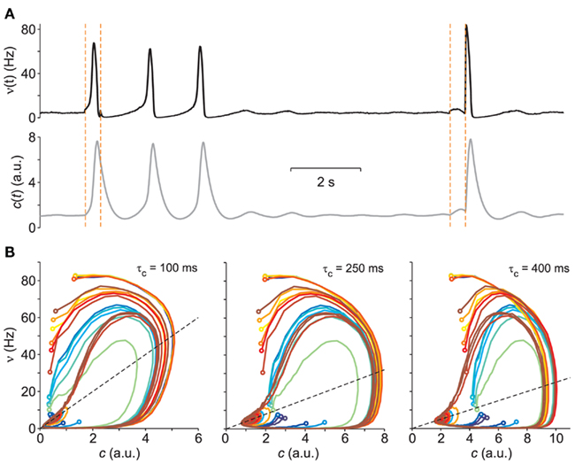
Figure 1. Vector field probing by external stimulation. (A) Population firing rate ν(t) from the simulation of a VIF neuron network (top, black trace) following sudden changes of Δν_ext (vertical dashed lines, see text for details). Bottom gray curve: adaptation variable c(t) numerically integrated from Eq. 2using the above ν(t) and assuming a value of τ_c = 250 ms. (B) Integrated network trajectories in the phase plane (c,ν) for three different values of τ_c. The 20 colored trajectories are given by 20 different initial conditions determined by the duration and intensity of the external stimulations. Dashed black lines are the nullclines. All trajectories approach the equilibrium point at ν = 5 Hz.

During the simulation we estimate the population firing rate ν(t) by sampling every Δt = 10 ms the spikes emitted by the whole network and dividing this value by NΔt.

2.3 Stimulation Protocol

The stimulation consists of varying the frequency ν_ext of the externally applied current: by varying its magnitude, the duration of the perturbation and the interval between subsequent stimuli, it is possible to reach almost all significant regions of the phase plane (c,ν). An example of a simple stimulation protocol is shown in Figure 1A: here, two stimuli have been applied each one consisting of two brief stimulations depicted as vertical dashed lines. During the stimulation, the frequency ν_ext of the external current is increased by Δν_ext and the state of the system at the end of the stimulation is taken as a new initial condition. The stimulation protocol we applied comes in two “flavors”: the first one (depicted for example in Figure 1A) consists of applying single stimuli separated by a fixed time interval T, with intensities randomly extracted from a Gaussian distribution with given mean and SD. The second one consists of applying a couple of “pulses” separated by a relatively short time period dt; subsequent stimuli doublets are again separated by a time T. In this case, while the first pulse is always excitatory (i.e., the mean of Δν_ext is positive), the second one may be either excitatory or inhibitory. In Table A1 in Appendix we summarize the values of the parameters used for the different in silico experiments.

2.4 Adaptation Dynamics Reconstruction

Given a fixed value of τ_c, the time course of c at population level can be obtained by numerically integrating Eq. 2. We used forward Euler’s method for all our simulations, resulting in an update formula that reads

where dt = 10 ms is the integration step corresponding to the sampling period of population discharge rate in the simulations. An example is shown in the lower part of Figure 1A.

2.5 Generation of the Fitting Data

For a given τ_c, starting from a set of trajectories composed of the measured discharge rate ν and the reconstructed adaptation variable c, we want to estimate the vector field of Eq. 2. By applying the finite difference method to the trajectories, we obtain values of G on an irregularly distributed set of points in the plane (c,ν). The reason for using a variable stimulation protocol – not only in terms of magnitude or duration of the perturbation, but also in terms of the interval between subsequent stimuli – lies in the fact that our final goal is to obtain trajectories that are as spread as possible over the phase plane: indeed, by uniformly covering the phase plane with trajectories, we can obtain an accurate estimation of the vector field of Eq. 2(De Feo and Storace, 2007).

2.6 Usage of Splines for Interpolation

In this work, we have used the MATLAB Spline Toolbox (The MathWorks Inc., Natick, MA, USA) to represent the functions that we want to estimate – namely, G, Φ^(eff), and τ_ν – on the whole phase plane. In particular, we have used “thin-plate smoothing” splines (Wahba, 1990) since they are capable of fitting and smoothing irregularly spaced grid of data. The resulting approximated surfaces are shaped by a smoothing factor, i.e., a value in the range [0, 1]: 0 corresponds to the least-squares approximation of the data by a flat surface, whereas 1 corresponds to a spline which interpolates the data. This parameter is critical especially in the estimation of G(c,ν), since too high values would lead to a very noisy vector field that in turn leads to numerical instability during the integration of Eq. 2. On the other hand, very low values of the smoothing factor correspond to extremely smooth G(c,ν) functions that are unable to replicate the oscillating behavior characteristic of the network, since the only attracting state is the equilibrium located at low frequencies. We have set the smoothing factor to 0.01 and 0.025 for networks composed of LIF and VIF neurons, respectively. We also remark that other values in the neighborhood of the ones we chose provide qualitatively analogous results, in terms of the behaviors that Eq. 2can reproduce.

2.7 Fit of the Nullcline in the Drift- and Noise-Dominated Regions

To evaluate coefficients in Eq. 10(see Section 3.3.1), which shape the nullcline at drift-dominated regime, we used the Optimization Toolbox included in MATLAB in order to fit the experimentally estimated curves by minimizing the following error measure:

where are the raw points that describe the nullcline and the sum runs over a certain number np of points. The optimization was repeated for 100 trials with different random initial guesses for the coefficients, in order to avoid local minima in which the optimization algorithm might be trapped: the best set of coefficients was then computed as the mean value of the coefficients resulting from the 10 optimization runs that gave lower error values. We have verified that, in the specific case under consideration, the lowest error values are associated to sets of coefficients that are very close to each other. As a consequence, our optimization procedure gives consistently the same results, indicating that the computed coefficients indeed correspond to a global minimum of the cost function.

On the ν = 0 axis, the field component G decays exponentially, i.e., the curve G(c,0) can be well described by an expression of the form G₀ exp(−c/γ). To obtain the values of the coefficients G₀ and γ we have first uniformly sampled the function G(c,0) using the spline representation of G – obtained with the procedure described in the previous section – and then fitted the values log(G(c,0)) with a first degree polynomial of the form a + bc. Consequently, the coefficients G₀ and γ are given by exp(a) and −1/b, respectively. The results of this simple fitting procedure are shown in Figure 4C.

2.8 Construction of the Bifurcation Diagram

To characterize the dynamical phases accessible to the used neuronal networks, we computed the bifurcation diagram reported in Figure 7 as follows. We first sampled the parameter plane (J_rec,g_c) on an irregular grid composed of 669 points: we chose this approach, instead of using a regularly spaced grid as commonly used practice in the bifurcation analysis of dynamical systems, both for the relative simplicity of this particular diagram and because of the prohibitive times that would be required to perform a more exhaustive analysis. Moreover, an irregular sampling of the parameter plane allowed us to increase the density of points across the bifurcation curves, such as those that mark the borders of the low-rate asynchronous state (LAS) & GO region. For each pair of parameters (J_rec,g_c) we simulated a network of LIF neurons for 50 s, as detailed previously. For the classification of the steady-state behavior, we discarded the first 10 s of simulation, during which ν_ext was exponentially increased to its steady-state value. The time course of ν is classified as asynchronous when no population bursts are present: in this case, it is possible to distinguish between low-rate and high-rate asynchronous attractor states by simply computing the mean of the instantaneous firing rate. If population bursts are present, the trace is classified as oscillating: in this case, we must distinguish whether the parameter pair is in the region where the limit cycle is the only stable attractor or in the region of coexistence between a stable limit cycle and a stable low-frequency equilibrium point. To do so, we compute the SD of the inter-burst intervals (IBIs): if such quantity is less than 0.2 times the mean of the IBIs, then we classify the parameter pair as in the region with only the stable limit cycle.

3 Results

The whole identification procedure is depicted in Figure 2: in the following, we shall discuss in greater detail each block present in the flow chart.

FIGURE 2

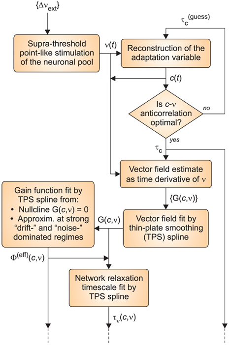
Figure 2. Flow chart of the identification algorithm. The procedure starts (top left corner) with the stimulation of the neuronal network through the protocol ({Δν_ext}) described in the Section 2. From the resulting instantaneous firing rate ν(t), the time course of the adaptation dynamics c(t) is carried out for different guess values of τ_c. The estimated τ_c is satisfying an optimality criterium based on the anti-correlation between c and ν. The trajectories (c(t),ν(t)) are then employed in the generation of the fitting data for the vector field component of interest ({G(c,ν)} on the phase plane). These sparsely distributed values are subsequently interpolated using a thin-plate smoothing spline. The resulting function G(c,ν) defined over the whole phase plane, together with various reference values and a fitting model for Φ^(eff), allow to reconstruct both the effective gain function Φ^(eff)(c,ν) and the network relaxation timescale τ_ν(c,ν).

3.1 Vector Field Reconstruction through Stimulation

We pursue the identification of network parameters following an opposite approach to the linear response to small perturbations. Here, we exploit the non-linearity of the network dynamics in order to have a phase space widely and spontaneously covered by trajectories, without driving it by means of an exogenous and continuous stimulation. As shown in Figure 1A, we deliver at random times (see Section 2 for details) brief “aspecific” stimulations to the network (vertical dashed lines). Depending on the state of the system, stimuli may or may not elicit a population burst, or more generally a large deviation from its equilibrium condition. This allows to overcome an obvious experimental constraint: since we are dealing with networks of neurons, we can not set their initial conditions at will. Here the state of the neuronal pool at the end of the stimulation is taken as starting point of a new relaxation dynamics for the system.

Besides, we assume that the population dynamics is effectively described by trajectories in the two-dimensional phase space (c,ν). Such dynamics is expected to follow the autonomous system in Eq. 2for a wide class of spiking neuron networks, as detailed in the Section 2. We consider as the only experimentally accessible information the instantaneous firing rate ν(t). The adaptation dynamics c(t) can be reconstructed from it, by using the second equation in system 2 (see Figure 1A, bottom plot and see Section 2 for details) for a chosen adaptation time constant τ_c.

Figure 1B clearly shows how relaxation trajectories following a stimulation critically depend on the chosen τ_c. Furthermore, it is also apparent how the non-linear dynamics of the network react to similar external stimulations in a state-dependent manner, bringing the system each time to a different initial condition (colored circles at the beginning of each trajectory in Figure 1B). From this point of view the complexity of the system helps the “exploration” of its phase space without resorting to complex stimulation strategies.

Starting from these effective trajectories, a two-dimensional vector field can be estimated. This is the first step toward the identification of the recovery time τ_c, the gain function Φ^(eff)(c,ν) and the neuronal relaxation timescale τ_ν(c,ν), that characterize the network dynamics at different levels of description.

3.2 Searching for the Optimal Vector Field

By further inspecting the trajectories reconstructed for different values of τ_c, we can observe that curve intersections mainly occur for small or long adaptation timescales. This is apparent looking at cyan-green and dark-red trajectories in the left and right panels of Figure 1B. Since system 2 describes a smooth vector field composed of ordinary differential equations, multiple solutions are not allowed, and this means that only one trajectory is expected to go through one point in the phase plane. Intersections are then not allowed and if they appear, it might be due to an incorrect value of τ_c or to an inadequate modeling of the system, for instance because more than two state variables are needed. Although the latter motivation seems the most likely due to the huge number of degrees of freedom (i.e., the number N = 20,000 of VIF neurons in the network here used), intersections practically disappear by setting τ_c = 250 ms (central panel of Figure 1B). Unsurprisingly, this is the exact value of τ_c set in the example simulations.

Starting from this qualitative intuition, we looked for an optimality measure of the adaptation timescale by inspecting the cross-correlation between the available population firing ν(t) and the reconstructed c(t). After a population burst, either spontaneous or induced by stimulation, adaptation is expected to reach a maximum level making almost quiescent the following firing activity of the network. This is the beginning of a recovery phase in which discharge rate increases as c(t) relaxes to its resting level c = 0. During this period c(t) and ν(t) are expected to be anti-correlated. We tested such relationship by computing the correlation degree between the measured population discharge rate and the reconstructed adaptation level for a wide range of values of τ_c. For each τ_c, we averaged c(t) and ν(t) in the 100 ms windows at fixed time lag Δt from the stimulation times. In Figure 3A, such correlation degrees are plotted for a set of Δt and each of them displays a maximum anti-correlation occurring at different τ_c, as highlighted by the black circles. Interestingly, the largest anti-correlation is obtained for an optimal Δt = 0.391 s, pointed out by the vertical dashed line in Figure 3B and roughly corresponding to the average duration of the elicited population bursts. The correlation degree for this optimal time lag has an absolute minimum for τ_c = 257 ms (see inset in Figure 3B). This value closely matches the parameter set in the simulation (τ_c = 250 ms), confirming the reliability of the optimality criterion here described.

FIGURE 3

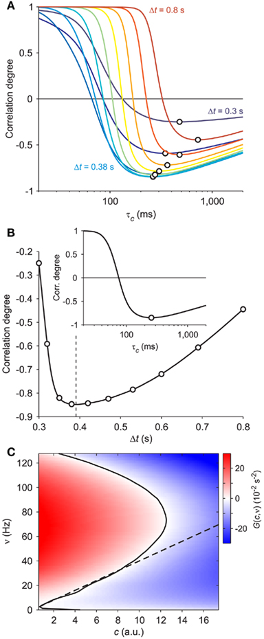
Figure 3. Optimal adaptation timescale and vector field estimate. (A) Dependence on τ_c of the correlation degree between average ν(t) and c(t) in the 100 ms periods at fixed time lag Δt from the beginning of reconstructed trajectories. Each curve correspond to a different Δt in the range [0.3, 0.8] s color coded from blue to red, respectively. Circles point out the maximum anti-correlation for each Δt. (B) Maximum anti-correlation versus Δt. Circles are the same as in (A) The dashed line at Δt = 0.391 s marks the minimum correlation degree. Inset: correlation degree versus τ_c for the optimal Δt. A circle marks the minimum at the optimal τ_c = 257 ms. (C) Estimated G(c,ν) in the phase plane (c,ν) setting τ_c to its optimal value: solid curve, nullcline ; dashed line, nullcline . Simulated network parameters as in Figure 1.

The estimate of τ_c, together with aspecific stimulations, allows for the reconstruction of a rich repertoire of trajectories filling the (c,ν) phase plane, as shown in Figure 1B. The time derivatives of such trajectories computed by applying a finite difference method provide a sparse estimate of the component of the vector field of system 2. In Figure 3C we illustrate the results of this step in the identification of the population dynamics. We smoothed the extracted field by a least square fit with a third-order spline surface (see Section 2.6 for details), eventually plotted as a color map. From the identified field components, we can work out the nullclines and , depicted as solid and dashed black curves in Figure 3C, respectively, which provide direct information on the accessible dynamical regime of the system.

3.3 Extracting Φ^(eff) from the Vector Field

Unfortunately, the availability of the vector field does not provide enough information to unambiguously identify the mean-field functions Φ^(eff) and τ_ν. In principle, an infinite set of functions can satisfy the expression for G(c,ν) in Eq. 2. To remove such degeneration, we resorted to some general model-independent hypotheses applicable to particular dynamical regimes of the neurons. Indeed, in strongly drift- and noise-dominated regimes we can extract some sparse information about the effective gain function, whereas no hints are available for intermediate regimes between the drift- and noise-dominated ones.

3.3.1 Hints from strongly “drift-dominated” regimes

In the presence of an intense barrage of excitatory synaptic events, the spike emission process is almost completely driven by the infinitesimal mean of the incoming current μ(c,ν) of Eq. 3. The generated spike trains are rather regular and at high frequency, because the membrane potential rapidly reaches the emission threshold following a constant refractory period τ₀. In this strongly “drift-dominated” regime with large μ(c,ν), inter-spike intervals (ISIs) are only mildly modulated by fluctuations of the input current (Tuckwell, 1988; Fusi and Mattia, 1999; Mattia and Del Giudice, 2002), and the membrane potential dynamics in Eq. 4reduces to that of a perfect integrator . The leakage current f(V) is neglected and the spike emission process becomes model-independent, and hence well suited also for biologically detailed descriptions. The time needed to reach the threshold θ starting from the reset potential H, together with τ₀, simply determine the average ISI and the corresponding output firing rate:

From the mean-field theory summarized in Eq. 3, μ(c,ν) is a linear combination of the synaptic event rate ν and the adaptation level c:

The coefficients μ₀, μ_c and μ_ν are unknown in our idealized in silico experiments, together with τ₀ and θ − H in Eq. 7. Nevertheless, we can estimate some of their ratios in the “drift-dominated” regime, relying on the extracted nullclines (see Figure 3C). Starting from the two previous expressions, Φ^(eff)(c,ν) = ν (which is valid on the nullcline ) implies the following relationship:

where c(ν) is the implicit function solving the nullcline definition equation G(c(ν),ν) = 0.

For clarity, Eq. 9can be rewritten as

where ν and c are the independent and dependent variables, respectively, and A = μ_0/μ_c, B = μ_ν/μ_c, C = (θ − H)/μ_c and D = τ₀ are the parameters to be estimated. Such coefficients can be obtained with a standard non-linear fit procedure detailed in Section 2.7. Figure 4A shows the best non-linear fit (red curve) of the data from the field identification (black curve, the same as that in Figure 3C), based on Eq. 9. Only the nullcline points above the top knee have been considered, because there the high output firing is expected to correspond to a strongly drift-dominated regime. Interestingly, the fit has reliably returned the theoretical refractory period τ₀ = 2 ms and a ratio μ_ν/μ_c = 1.12 s, very close to the expected μ_ν/μ_c = 1.27 s. Although τ₀ is estimated at drift-dominated regime, it is assumed that its value does not change for different (c,ν), accordingly to the theoretical description adopted.

FIGURE 4

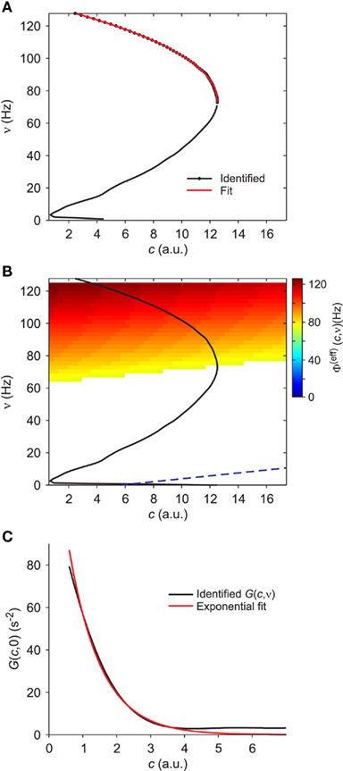
Figure 4. Extraction of reference values for Φ^(eff). (A) Fit of the nullcline (black curve and dots, the same as Figure 3C) with a theoretical guess (red curve) obtained from a general expression valid at drift-dominated regimes of firing activity for a wide class of spiking neurons (see text for details). (B) Φ^(eff)(c,ν) extracted starting from theoretical fit in B. Colors code output firing rates. White region is where Φ^(eff) has no reference values. Below the blue dashed line Φ^(eff) = 0. Black curve as in (A,B). (C) G(c,ν) at ν = 0 (black) and its fit G₀ exp(− c/γ) (red, G₀ = 140/s² and γ = 0.94). Simulated network parameters as in Figure 1.

The assumption of an effective gain function depending only on the mean current μ given by the linear combination in Eq. 8, yields a simple geometric property: Φ^(eff) is constant when computed on a straight line parallel to ν = (μ_c/μ_ν)c in the plane (c,ν) (see Eqs. 7 and 8). From the previous non-linear fit we know the slope of those lines. Besides, the red nullcline branch shown in Figure 4A provides the reference values in this drift-dominated regime for the effective gain function, being there Φ^(eff) = ν. Both these considerations allow us to extract Φ^(eff)(c,ν) in the wide range of the phase plane depicted in Figure 4B. The colored region codes for the identified output firing rate, while the remaining white area is where no hints are available for Φ^(eff).

3.3.2 Hints from strongly “noise-dominated” regimes

On the other hand, Figure 4C shows that the identified field component G on the ν = 0 axis (black curve) well fits the exponential G₀ exp(− c/γ) (red curve; see Section 2.7). Furthermore, from Eq. 2the gain function on the same axis is Φ^(eff) = τ_νG, such that Φ^(eff) = 0 when G(c,0) = 0. The exponential decay of the output discharge rate for increasing adaptation level is a general feature and can be explained noticing that the spike emission process mainly due to large random fluctuations of incoming synaptic current: a “noise-driven” firing regime (Fusi and Mattia, 1999). In the absence of a recurrent feedback (ν = 0), synaptic activity is elicited by spikes from neurons outside the local network. The superposition of enough excitatory events in a small time window may overcome the self-inhibition current dependent on c. The larger c, the lower the likelihood of having a strong enough depolarization capable of causing the emission of a spike. Similarly to the escape problem of a Brownian particle from a potential well (Risken, 1989), the output discharge rate depends exponentially on the distance of the membrane potential from the emission threshold, which is in turn proportional to the current drift μ (Tuckwell, 1988). Conservatively, we then can say that for c > 6γ, Φ^(eff)(c,0) ≃ 0. The same approximation holds for the points of the phase plane where μ(c,ν) < μ(6γ,0). The top boundary of such region is the blue dashed line in Figure 4B: its slope is μ_c/μ_ν, as previously estimated.

3.3.3 Extracting the whole Φ^(eff) surface

The two regions of the phase plane that provide an estimate of the effective gain function, together with the nullcline Φ^(eff) = ν, provide a sparse representation of the whole Φ^(eff) surface because no hints are available for intermediate regimes between the drift- and noise-dominated ones. Besides, the gain function at fixed c is expected to be regular and with a sigmoidal shape. Indeed, randomness of the input current grants the smoothness of the surface even for drifts μ(c,ν) close to a rheobase, when the neurons stop firing and Φ^(eff) shows a discontinuity of the derivative (see for instance Gerstner and Kistler, 2002; La Camera et al., 2008). Under noise-driven spiking regimes such discontinuity disappears, because current fluctuations allow the emission of spikes even for values of μ lower than the rheobase (for review, see Burkitt, 2006; La Camera et al., 2008). Hence, assuming fluctuating synaptic currents usually observed both in vivo and in vitro, we model the whole Φ^(eff) surface as a “thin-plate smoothing spline” (Wahba, 1990) with a rigidity parameter minimizing the difference between the model and the available estimates of the gain function (see Section 2.6 for details). The fitting result is shown in Figure 5A. In Figure 5B Φ^(eff)(c,ν) sections at different adaptation levels show the almost threshold-linear behavior of the VIF neurons (Fusi and Mattia, 1999) and the smoothness around the rheobase current, where output rate approaches the “no firing” region. It is also apparent the effect of the self-inhibition due to the considered adaptation mechanism: for increasing values of c, the gain function is almost rigidly shifted to the right, thus reducing the output discharge rate in response to the same input ν.

FIGURE 5

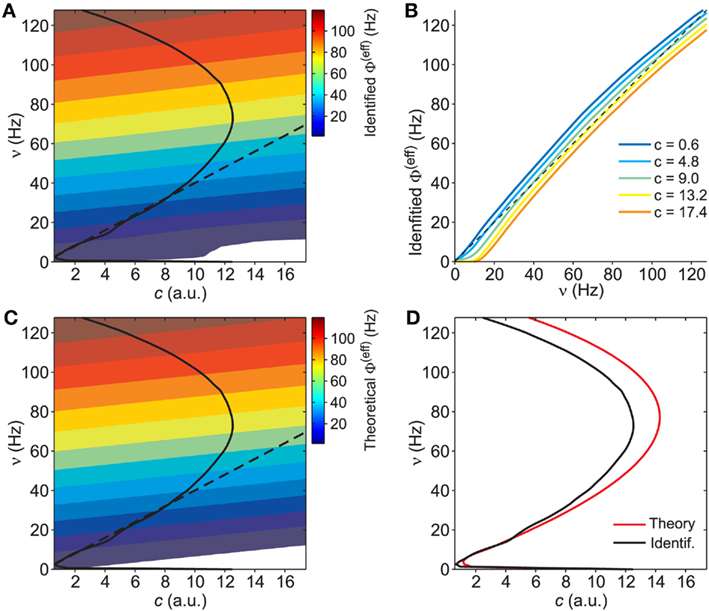
Figure 5. Identification of the gain function Φ^(eff). (A) Contour plot of the identified gain function Φ^(eff)(c,ν) starting from the reference values extracted in Figure 4 (white region, Φ^(eff) < 0.5 Hz). Solid and dashed black curves, the same nullclines of the vector field as in Figures 3 and 4. (B) Identified Φ^(eff) sections at different c (see inset for color code). Black dashed line, Φ^(eff) = ν. (C) Contour plot of Φ^(eff) from mean-field theory for model parameters as in Figure 1 (white region, Φ^(eff) < 0.5 Hz). Black curves as in (A). (D) Theoretical nullcline Φ^(eff) = ν (red) versus the one from the identified G(c,ν) black, the same as in (A,C).

The reliability of the identification is proved by the close resemblance between the estimated Φ^(eff) and the theoretically expected surface shown in Figures 5A,C, respectively. A deeper inspection matching the nullclines Φ^(eff)(c,ν) = ν emphasizes the existence of a significant discrepancy at high output discharge rates, where in Figure 5D theoretical and identified nullclines (red and black curves, respectively) slightly diverge. Such mild difference should not be attributed to a failure of the identification process, but rather to the limitations of the mean-field theory. Indeed, the diffusion approximation requires small post-synaptic potentials and large input spike rates. At drift-dominated regimes, such constraints are more stringent to accurately describe the probability distribution of the membrane potentials of the neuronal pool (Sirovich et al., 2000). Another possible source of error is the quenched disorder (van Vreeswijk and Sompolinsky, 1996), which we have not taken into account in our dimensional reduction. The variability in the number of synaptic contacts among the neurons in the network induces a distribution of firing rates, which in turn affects the moments of the input current. Such additional variability may have a potential role at noise-dominated regime. Fortunately, in this region of the phase plane in Figure 5D theoretical and identified nullclines match well.

3.4 Identification of the Network Timescale τ_ν

Now that we have a reliable gain function Φ^(eff) over the whole phase plane (c,ν), we can directly obtain the timescale function τ_ν from Eq. 2with the identified field G:

Because in this expression small values of G yield large uncertainties in τ_ν, we avoid to consider the above estimate in the region of the phase plane where |G| < 800/s², around the nullcline . Also in this case, the missing values of τ_ν are recovered using a thin-plate smoothing spline fitting of the available edges of the surface (see Section 2 for details). The resulting τ_ν(c,ν) is plotted in Figure 6A. Interestingly, the sections of this surface at increasing adaptation level c show the existence of τ_ν maxima for increasing output rate ν, as shown in Figure 6B. A plateau at high frequencies is also apparent. At least qualitatively, both these features confirm the theoretical predictions in Gigante et al. (2007), where an activity-dependent relaxation timescale has been reported for spiking neuron networks (see Section 4).

FIGURE 6

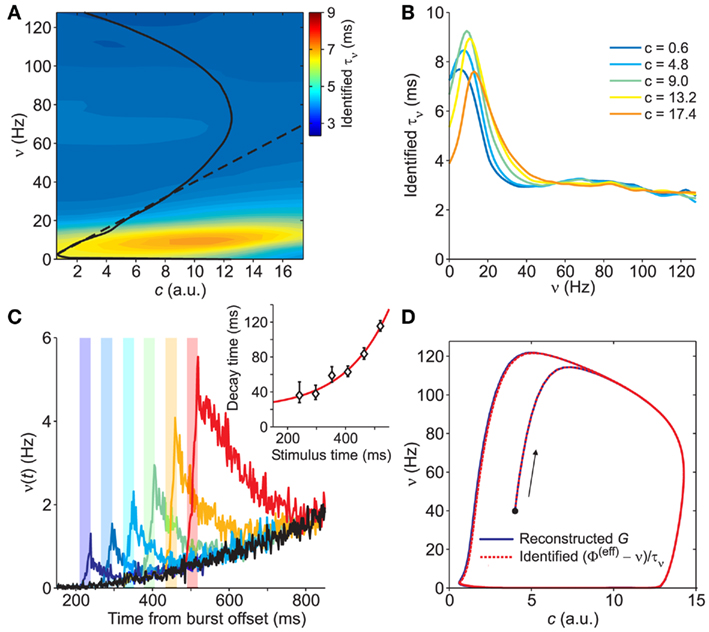
Figure 6. Identification of the network timescale function τ_ν. (A) Contour plot of the identified τ_ν(c,ν), obtained from the gain function Φ^(eff) in Figure 5A and the field component G in Figure 3C. The black curves are the same nullclines as in the previous figures. (B) Sections of the identified τ_ν for different values of c (see inset for color code). (C) Network activity response to the same external stimulation (vertical color bars) at different times. Simulations start from the same initial condition. Black trace: network activity without stimulation. Inset: time constants of the exponential decays in approaching the unperturbed condition after stimulation. Red curve: best fit y = 3.1 exp(6.6x) + 20 for the decay time versus stimulus time. (D) Trajectories resulting from the numerical integration of Eq. 2with component given by the reconstructed and smoothed G in Figure 3C (solid blue line) and by (Φ^(eff) − ν)/τ_ν with identified functions shown in (A) and in Figure 5A (dashed red line), respectively. Black dot: common initial condition. Arrow: direction of increasing time.

The estimated relaxation timescale (less than 10 ms) highlights how fast the network dynamics is compared to the average duration of the population bursts (hundreds of milliseconds) and to the IBIs (seconds). We stress this because the non-linear network dynamics is a complex combination of the state of the system, the network properties and the neuronal and synaptic microscopic parameters. Simply looking at the activity decay following an external stimulation does not directly provide an easy way to infer such network timescales, as shown in Figure 6C. The asymptotic value of the time constant of the exponential activity decay following stimulations just after the last population burst gives only a rough indication (see inset of Figure 6C).

Eventually, we complete the identification process by testing the dynamics of the system following Eq. 2by using the estimated Φ^(eff), τ_ν and τ_c. The numerical integration of such system returns orbits in the phase plane in a remarkable agreement with those obtained using the field component G resulting from the in silico experiments (see Figure 6D).

3.5 The Microscopic Level across Bifurcations

So far, we introduced our middle-out and model-driven identification approach probing its effectiveness on a relatively simple in silico experiment, i.e., a network of homogeneous VIF neurons. Nevertheless, the theoretical bases of the method are rather general, and make it suited also for more detailed and sophisticated spiking neuron models, and eventually to controlled biological preparations like in vitro brain slices and cultured neuronal networks. Furthermore, the dimensional reduction of the network dynamics in Gigante et al. (2007), on which the method presented here relies, is independent on the dynamical activity regime, even in the presence of a rich repertoire of collective behaviors in the phase diagram.

3.5.1 Bifurcation diagram of LIF neuron networks

Here, we exploit such potential by devising an in silico experiment in which a network of excitatory LIF neurons changes its dynamical behavior after modulation of some microscopic parameters. As in an in vitro experiment, we probe in simulation the spontaneous activity of the neuronal pool when some “virtual” glutamate receptor agonist and/or antagonist modulates the strength J_rec of the recurrent synaptic couplings. Besides the regulation of the excitability of the network, we simultaneously change the intensity of the self-inhibition responsible for the SFA, by varying g_c.

Hence, we carry out a bifurcation analysis of the network activity sampling intensively the plane (J_rec, g_c) (see Section 2.8 for details). The result of this bifurcation analysis is summarized in Figure 7A, where different colors denote different asymptotic dynamical behaviors. In the LAS (green region), the only stable attractor is an equilibrium point, corresponding to low-frequency network activity (example in Figure 7B: J_rec = 0.102 mV and g_c = 21 mV/s). The GO region (cyan region) is where the only stable attractor is a limit cycle corresponding to periodic population bursts (example in Figure 7D: J_rec = 0.112 mV and g_c = 21 mV/s). In the thin orange region (labeled as LAS & GO), two stable attractors coexist, namely a low-frequency equilibrium and a limit cycle (Figure 7C: J_rec = 0.106 mV and g_c = 21 mV/s). Finally, the high-rate asynchronous state (HAS, pink region) is where the only stable attractor is an equilibrium point, corresponding to high-frequency network activity (Figure 7E: J_rec = 0.086 mV and g_c = 21 mV/s). The only bistable state – at least for the considered parameter sets – is LAS & GO: in the deterministic infinite-size limit, the system would end up on one of the two stable attractors depending on the initial condition and would switch only after the application of an external stimulation; in the case of realistic neuronal networks, finite-size fluctuations due to endogenous noise sources can induce spontaneous switches between states. We point out that in Figures 7B,E, simulations display also the initial transient evolution of the population discharge rate ν(t), during which the externally applied current ν_ext exponentially adapt, increasing from 0 to its steady-state value.

FIGURE 7

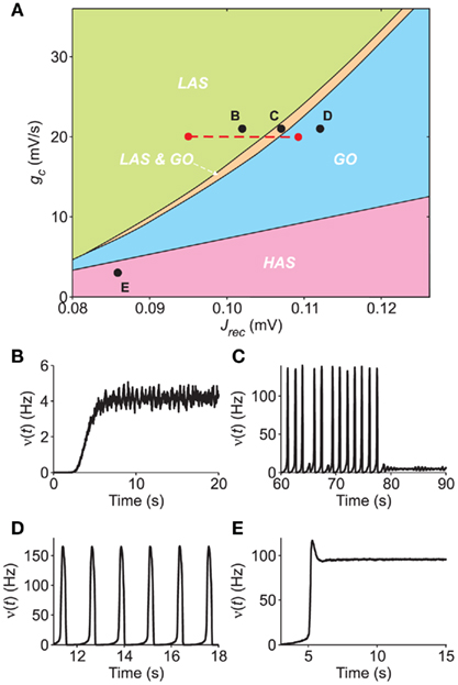
Figure 7. Bifurcation diagram of a simulated network of excitatory LIF neurons. (A) Section of the bifurcation diagram in the plane (J_rec,g_c) displaying the different dynamical regimes observed in the simulations: LAS, single attractor low-firing asynchronous state (green); LAS & GO, coexistence of LAS and a metastable limit cycle where the network shows global oscillations (orange); GO, only periodic population bursts occur; HAS, single attractor high-firing asynchronous state. Red dashed line, region explored in Figure 8. (B–E) Examples of population activity from simulations in the different dynamical regimes of the bifurcation diagram [see respectively labeled black dots in (A)]. Simulated networks are composed of 20,000 excitatory LIF neurons.

It is interesting to note the similarities of the carried out bifurcation analysis with an analogous bifurcation diagram reported in Gigante et al. (2007) for excitatory VIF networks. At least qualitatively, similar dynamical states are situated in the same relative positions. HAS regimes have been found for relatively mild SFA, whereas for higher values of g_c increasing synaptic strength yields successively to single asynchronous states (LAS), then to coexistence of two stable states (LAS & GO) and eventually to periodic population bursting regimes (GO).

3.5.2 Microscopic features from mesoscopic identification

Taking into account the information provided by the diagram in Figure 7, we exploit the robustness of our identification method with respect to the crossing of bifurcation boundaries. To this end, we fix g_c = 20 mV in order to span a reasonably large interval of LAS & GO behavior and sweep J_rec in the range [0.096, 0.108]mV (red dashed line in panel A of Figure 7). For each value of J_rec, we apply the method described in the previous sections to estimate G, τ_c, Φ^(eff), and τ_ν.

The results are presented in Figure 8: the top panel shows the shape of the nullcline as a function of J_rec. In particular, as J_rec is increased, the shape of the nullcline changes and the equilibrium point corresponding to the intersection with the nullcline (black dashed line in panel A) loses its stability at the frontier between the LAS & GO and GO regions (see Figure 7). The limit cycle that appears by crossing this (subcritical) Hopf bifurcation is unstable and exists in the LAS & GO region. At the border between the LAS and LAS & GO regions the unstable cycle collides, through a fold bifurcation of cycles, with the stable limit cycle that describes the oscillatory behavior of the network shown in both the LAS & GO and GO regions. This kind of behavior is quite standard in many neuron models and is related to the presence of a Generalized Hopf bifurcation at the tip of the LAS & GO region.

FIGURE 8

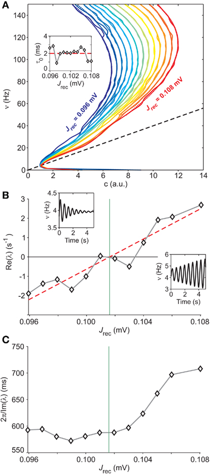
Figure 8. Extracting microscopic features from mesoscopic identification. (A) Nullclines of the identified field component G from LIF network simulations at different levels of recurrent synaptic excitation J_rec, spanning the red dashed line in Figure 7A (see colored labels, J_rec sampled at steps of 1 mV). Adaptation level fixed at g_c = 20 mV/s. Dotted colored curves: fitted nullcline approximations at drift-dominated regime as in Figure 4A. Black dashed line: nullcline . Inset: estimated absolute refractory period τ₀ versus J_rec; dashed red line, expected value. (B) Correlation between J_rec and the real part of the eigenvalues λ of the Eq. 2Jacobian, using the identified G(c,ν) around the equilibrium point ∼(1,4 Hz). Red dashed line: linear regression (p < 10⁻³, t-test). Green vertical line: Hopf bifurcation predicted by the linear fit. Insets: examples of ν(t) dynamics for Re(λ) < 0 (top left) and Re(λ) > 0 (bottom right) close to the equilibrium point. (C) Oscillation periods of ν(t) given by inverse Im(λ). Oscillations are damped only at the left of the Hopf bifurcation (green vertical line).

The approximation at drift-dominated regime for the nullcline in Eq. 9is also well suited for networks of LIF neurons, as testified by the remarkable match between dotted and solid nullclines in Figure 8A, which extends well below their top knees. This confirms the expected wide applicability of the functional expression for the nullcline to a wide class of spiking neuron models. The identification of the adaptation timescale τ_c provides also for these networks values very close to the corresponding parameters set in the simulations, providing a further confirmation of the reliability of our approach for different models and dynamical regimes.

At this point, having identified the field component G(c,ν) and the functions Φ^(eff) and τ_ν for a set of different values of J_rec, we investigate the relationship between the mesoscopic and the microscopic description levels of the system. We focus on the Hopf bifurcation described above. The mean-field theory for the dynamics of spiking neuron networks (Mattia and Del Giudice, 2002; Gigante et al., 2007) establishes a direct relationship between the Jacobian’s eigenvalues λs for Eq. 2and the slope of the gain function Φ^(eff) around equilibrium points. If Im(λ) ≠ 0, the linearized dynamics for Eq. 2yields

where ∂_νΦ^(eff) and τ_ν are computed in (c*,ν*), an equilibrium point for Eq. 2. Since J_rec always multiplies ν in the expression 1 for the moments of the input current, for small changes of J_rec as in the case under investigation, the slope of Φ^(eff) in the ν direction will be proportional to the average synaptic efficacy, i.e., ∂_νΦ^(eff) ∝ J_rec. Hence, Re(λ) is expected to linearly depend on J_rec according to Eq. 11, as we found numerically from the identification in Figure 8B (gray curve). In this case, the equilibrium point is at low-ν and c, where the nullclines and intersect. The system undergoes the Hopf bifurcation (vertical green line) where the linear fit (red dashed line) crosses x-axis in Figure 8B. This occurs at a critical J_rec = 0.1015 mV very close to the theoretically expected value J_rec = 0.1048 mV, provided by Eq. 11. Imaginary part of λs (see Figure 8C) further confirms the complex relationship between the period of the population oscillations (gray curve) and τ_c, and hence the need for ad hoc identification strategies for τ_c, like the one we proposed.

Another example of microscopic extraction is provided by the nullcline approximation at drift-dominated regime in Eq. 9. One of the fitted parameters is the absolute refractory period τ₀, which in our simulations is set to 2 ms. The inset in Figure 8A clearly shows the accuracy of its identification, which only mildly fluctuates for different J_rec, even if the network is crossing a bifurcation boundary.

We conclude this section remarking the relevance of these results. Although we started inspecting an intact network of spiking neurons, the devised model-driven approach provides tools to estimate microscopic features like synaptic coupling J_rec and absolute refractory period τ₀. This simply relying on the mesoscopic description of the system given by the identified functions Φ^(eff) and τ_ν of the neuronal pool.

4 Discussion

In this study, we presented a method to identify the network dynamics of a homogenous pool of interacting spiking neurons with SFA. We analyze the spontaneous relaxation time course of the population discharge rate without considering any linearization. The non-linearity of the activity dynamics is exploited by supra-threshold stimulations in order to have a complete description of the system. Furthermore, the network is investigated as a whole, as opposed to a bottom-up approach characterizing the system starting from its microscopic elements. This mesoscopic description projects the network dynamics in the low-dimensional state space of the instantaneous discharge rate ν(t) and the adaptation level of the adaptation mechanism c(t), as suggested by a recent mean-field theory development (Gigante et al., 2007). This model-driven approach allows us to make direct links to the microscopic level available. Indeed, we show how the timescale τ_c of the SFA together with the absolute refractory period τ₀ and the average synaptic efficacy J_rec can be faithfully extracted.

4.1 A New Way to Probe the System Dynamics

Networks are probed by eliciting strong reactions. To this aim, aspecific and supra-threshold stimulations are delivered, following an approach that significantly differs from those used to study the linear response properties of biological systems (Knight, 1972b; Sakai, 1992; Wright et al., 1996). Networks are then driven in “uncommon” dynamic conditions in order to exploit the non-linear activity relaxation outside the stimulation period. This “out-of-stimulation” identification evidences the bona fide network dynamics, by avoiding any artifacts due to artificial inputs, like sinusoidal or randomly fluctuating intra- or extracellular electric field changes (Chance et al., 2002; Rauch et al., 2003; Giugliano et al., 2004; Higgs et al., 2006; Arsiero et al., 2007). Besides, we have shown how the system reaction is state-dependent, so that the same stimulation may elicit very different responses. This is an added value, yielding to a reduced complexity of the stimulation protocol in order to have a dense coverage of the phase plane. Such complexity is in turn delegated to the non-linear dynamics of the network activity.

Aspecific stimulations involving a whole pool of neurons clearly resemble the well known electrical microstimulation often adopted in neurophysiology to probe and understand how the nervous tissue works (see for review Cohen and Newsome, 2004; Tehovnik et al., 2006). This is one of the main reasons why we have resorted to this approach, envisaging a wide applicability even in less controlled experimental conditions, such as those where the intact tissue is investigated.

To this aim, it is apparent why we have chosen to watch the system dynamics only through the “keyhole” of the population discharge rate, without resorting to other microscopic information available in our in silico experiments. We assumed to have access only to multi-unit spiking activity (MUA) from local field potentials (LFP), together with electrical microstimulation, in order to coherently investigate the network as a whole adopting a pure “extracellular” approach.

4.2 Robustness of the Identification to Phase Transitions

A major improvement provided by our model-driven approach in the identification of neuronal network dynamics is not only its ability to deal with and exploit the intrinsic non-linearities of a system with feedback and adaptation, but also its capability to faithfully extract the features of the system in a manner which is almost independent of the particular dynamical phase expressed, as we have shown in Figure 8. This is a novelty with respect to other modeling approaches that rely on input linear filtering and non-linear input–output relationships with feedback like generalized linear models (Paninski et al., 2007) and linear–non-linear cascade models (Sakai, 1992; Marmarelis, 1993). Such theoretical frameworks, although well suited to describe non-linear biological systems, to the best of our knowledge have never proved their applicability across phase transitions between dynamical regimes.

The robustness with respect to the crossing of bifurcation boundaries may result to be of great interest in understanding the neuronal mechanisms behind the activity changes of the nervous tissue under controlled experimental conditions. Developing neuronal cultures in vitro provides an ideal experimental setup because different patterns of collective activity stand out, depending on the developmental stage (Segev et al., 2003; van Pelt et al., 2005; Chiappalone et al., 2006; Soriano et al., 2008). Pharmacological manipulations are also appealing because they are capable to drive neuronal cultures in different dynamical states by selectively modulating synaptic and somatic ionic conductances (see for instance Marom and Shahaf, 2002). Brain slices in vitro may provide another applicability domain for our identification approach, for instance to investigate the neuronal substrate of epilepsy onset (Gutnick et al., 1982; Sanchez-Vives and McCormick, 2000; Sanchez-Vives et al., 2010), even though the structure of the tissue and the cell type heterogeneity may force the assumptions our method relies on, limiting its effectiveness.

4.3 Activity-Dependent Gain Function and Relaxation Timescale

As shown in Figure 5, our model-driven identification makes the input–output gain function Φ^(eff) of the neurons in a network available. This function characterizes the capability of the neurons to modulate and transmit the input activity from other computational nodes, conveying sensorial or other information. The relevance of this response function is evidenced by the experimental effort put into extracting it, typically by injecting into neurons suited input currents and measuring the output discharge rates (Chance et al., 2002; Rauch et al., 2003; Giugliano et al., 2004; Higgs et al., 2006; Arsiero et al., 2007; see La Camera et al., 2008 for a review). The input to Φ^(eff) is the instantaneous frequency of the spikes bombarding the dendritic tree of the neurons and not the synaptic current, as often considered. This yields to a clear advantage: it makes homogeneous the input and the output, incorporating the possible unknown relationship between pre-synaptic firing rate and input synaptic current. A simplification which helps to deal with closed loops, where the neuronal network output is fed-back as input.

Besides, the firing rate ν is not the only input to Φ^(eff): because of the SFA mechanism, Φ^(eff) depends also on the average adaptation level c. As summarized in the Section 2, c affects the average input current as an additional inhibitory current, which in turn rigidly shifts the neural gain function. This is still a rather rough approximation, and the “effective” gain function Φ^(eff) improves it, by introducing a further activity-dependent modulation (Gigante et al., 2007): a perturbation that accounts for the distribution of membrane potentials in the neuronal pool, consistently to what has been previously argued for isolated neuron models (Benda and Herz, 2003).

Moreover, the system identification allowed us to verify the existence of an activity-dependent relaxation timescale τ_ν(c,ν) for the network dynamics, as expected from recent theoretical developments (Gigante et al., 2007). Interestingly, a similar activity-dependent timescale has been recently introduced in a linear–non-linear cascade modeling framework as a phenomenological way out to obtain a more accurate description of the output firing of neurons to time-varying synaptic input (Ostojic and Brunel, 2011). The ability of the network to exhibit state-dependent reaction times may be of direct biological relevance (Marom, 2010), and further extend the standard rate model framework a la Wilson and Cowan (1972).

4.4 Limitations and Perspectives

We tested the robustness and generality of our methodology on relatively simple and well controlled in silico experiments, reporting remarkably good agreement between theoretically expected and identified dynamics. In particular, we found a slight difference in the nullcline Φ^(eff)(c,ν) = ν (see Figure 5D) likely due to a failure of the diffusion approximation at strong “drift-dominated” regimes of spiking activity, usually those corresponding to high discharge rates. Furthermore, we obtained a τ_ν(c,ν) with a shape qualitatively similar to what is predicted by the theory (see Figure 1 in Gigante et al., 2007), showing a maximum timescale and a plateau at very high frequencies. The maxima of the theoretical τ_ν are located along the nullcline ν = c/τ_c, whereas the identified maxima seem to stand on a straight line on which the average input current remains constant: ν = μ_c/μ_νc. Such a difference may be attributed to the failure of the assumption to have a small enough acceleration of the firing rate. Indeed, acceleration has its maximum value close to the nullcline , where the onset and the offset of the population bursts take place (Gigante et al., 2007). Paradoxically, should this be confirmed, the model-driven identification would provide a more reliable system description than the theoretical one.

But how much do the assumptions underlying the theoretical framework constrain the applicability of our method to more complex and realistic scenarios? Provided that the mean-field and diffusion approximations are well suited to describe the biological system under investigation, the dimensional reduction we adopted is expected to have a wide applicability. Indeed, the requirements of having a large number of synaptic inputs on the neuronal dendritic trees and small enough post-synaptic potentials compared to the neuronal emission threshold well fit the characteristics of the cerebral cortex (Amit and Tsodyks, 1991; Braitenberg and Schüz, 1998). The expressions for the gain function Φ^(eff) at strongly drift- and noise-dominated regimes, introduced and used in Figure 4, are rather general. Besides, we assumed the infinitesimal mean μ(c,ν) of the synaptic current to be a linear combination of ν and c, but even this constraint can be replaced by other non-linear expressions (Brunel and Wang, 2001), if more consistent with the biological background.

Also, our theoretical framework does not consider realistic synaptic transmissions: in particular, an instantaneous post-synaptic potential occurs at the arrival of a pre-synaptic spike, neglecting the typically observed ionic channel kinetics. Nevertheless, recent advances in the study of the input–output linear response of the IF neurons have proved that realistic synaptic transmission brings neurons to have fast responses to input changes (Brunel et al., 2001; Fourcaud and Brunel, 2002). Hence, we expect only a mild perturbation of the functions Φ^(eff) and τ_ν due to synaptic filtering, at least for relatively fast synapses like AMPA and GABA_A. For such gating variables with slower kinetics like NMDA receptors, we can include an additional dynamic variable that describes synaptic integration on time scales longer than τ_ν (Wong and Wang, 2006). This additional degree of freedom can be handled similarly to the dynamics of c in Eq. 2, by extending the optimization strategy summarized in Figure 3 to a multi-dimensional space of the decay constants.

Such a generalization to multiple timescales of the synaptic input could in principle be used to relax the constraint in modeling the fatigue variable c(t) with a simple first-order dynamics. More complex fatigue phenomena could be embodied as a cascade of first-order differential equations mimicking the wide repertoire of ionic channel kinetics (Millhauser et al., 1988; Marom, 2009), including also additional adaptation and recovery mechanisms (La Camera et al., 2006; Lundstrom et al., 2008). Furthermore, we adopted a simplified spike-driven model for c-dependent self-inhibition, assuming in particular a coupling term g_c independent from the neuron membrane potential. More biologically inspired voltage-dependent ionic conductances would yield the moments of the input current to be non-linear functions of c and ν. Such non-linearities could in turn be “absorbed” in the expressions for Φ^(eff) and τ_ν, hence making our identification approach yet usable.

The identification strategy and the in silico experiments reported here do not take into account networks composed of different neuronal pools: we have considered only a homogenous population of excitatory IF neurons. Hence, a question arises: can our method be extended to deal with more than one interacting neuronal pool? Depending on the experimental accessibility to the separate firing rates, for instance of the inhibitory and excitatory populations, different strategies can be adopted. If a mix of discharge frequencies is available, the identification should rely on a generalized theory resorting to a kind of “adiabatic” approximation such that inhibitory activity rapidly adapts to time-varying excitatory firing rates (Mascaro and Amit, 1999; Wong and Wang, 2006). On the other hand, if experimental probes are available to measure separately the firing rates and to deliver independent stimulations, the identification could be managed extending our approach to cope with a high-dimensional phase space and thus more than one Φ^(eff) and τ_ν functions. A different approach, if experimentally viable, could be to isolate the subnetworks and identify them using the original method, and eventually inferring the restored inter-population connectivity. To this aim, correlation-based approaches originally applied to small neuronal networks (Schneidman et al., 2006; Pillow et al., 2008), could be successfully used in this context by considering as basic computational node the identified neuronal pools.

Conflict of Interest Statement

The authors declare that the research was conducted in the absence of any commercial or financial relationships that could be construed as a potential conflict of interest.

Acknowledgments

We thank P. Del Giudice for stimulating discussions, R. Cao for a careful reading of the manuscript and Reviewers for helpful comments. Maurizio Mattia is supported by the EU grant to the CORONET project (ref. 269459).

References

Abbott, L. F., and van Vreeswijk, C. (1993). Asynchronous states in networks of pulse-coupled oscillators, Phys. Rev. E 48, 1483–1490.

CrossRef Full Text

Amit, D. J., and Brunel, N. (1997). Model of global spontaneous activity and local structured activity during delay periods in the cerebral cortex, Cereb. Cortex 7, 237–252.

Pubmed Abstract | Pubmed Full Text | CrossRef Full Text

Amit, D. J., and Tsodyks, M. (1991). Quantitative study of attractor neural network retrieving at low spike rates: I. substrate–spikes, rates and neuronal gain, Network 2, 259–273.

CrossRef Full Text

Arsiero, M., Lüscher, H.-R., Lundstrom, B. N., and Giugliano, M. (2007). The impact of input fluctuations on the frequency-current relationships of layer 5 pyramidal neurons in the rat medial prefrontal cortex, J. Neurosci. 27, 3274–3284.

Pubmed Abstract | Pubmed Full Text | CrossRef Full Text

Badel, L., Lefort, S., Brette, R., Petersen, C. C. H., Gerstner, W., and Richardson, M. J. E. (2008). Dynamic I-V curves are reliable predictors of naturalistic pyramidal-neuron voltage traces, J. Neurophysiol. 99, 656–666.

Pubmed Abstract | Pubmed Full Text | CrossRef Full Text

Benda, J., and Herz, A. V. M. (2003). A universal model for spike-frequency adaptation, Neural Comput. 15, 2523–2564.

Pubmed Abstract | Pubmed Full Text | CrossRef Full Text

Bhattacharjee, A., and Kaczmarek, L. K. (2005). For K+ channels, Na+ is the new Ca2+, Trends Neurosci. 28, 422–428.

Pubmed Abstract | Pubmed Full Text | CrossRef Full Text

Braitenberg, V., and Schüz, A. (1998). Cortex: Statistics and Geometry of Neuronal Connectivity, 2nd Edn. Berlin: Springer.

Brunel, N., Chance, F. S., Fourcaud, N., and Abbott, L. F. (2001). Effects of synaptic noise and filtering on the frequency response of spiking neurons, Phys. Rev. Lett. 86, 2186–2189.

Pubmed Abstract | Pubmed Full Text | CrossRef Full Text

Brunel, N., and Hakim, V. (1999). Fast global oscillations in networks of integrate-and-fire neurons with low firing rates, Neural Comput. 11, 1621–1671.

Pubmed Abstract | Pubmed Full Text | CrossRef Full Text

Brunel, N., Hakim, V., and Richardson, M. J. E. (2003). Firing-rate resonance in a generalized integrate-and-fire neuron with subthreshold resonance, Phys. Rev. E Stat. Nonlin. Soft Matter Phys. 67(5 Pt 1), :051916.

Pubmed Abstract | Pubmed Full Text | CrossRef Full Text

Brunel, N., and Wang, X.-J. (2001). Effects of neuromodulation in a cortical network model of object working memory dominated by recurrent inhibition, J. Comput. Neurosci. 11, 63–85.

Pubmed Abstract | Pubmed Full Text | CrossRef Full Text

Burkitt, A. N. (2006). A review of the integrate-and-fire neuron model: I. Homogeneous synaptic input, Biol. Cybern. 95, 1–19.

Pubmed Abstract | Pubmed Full Text | CrossRef Full Text

Casti, A. R. R., Omurtag, A., Sornborger, A., Kaplan, E., Knight, B., Victor, J., and Sirovich, L. (2002). A population study of integrate-and-fire-or-burst neurons, Neural Comput. 14, 957–986.

Pubmed Abstract | Pubmed Full Text | CrossRef Full Text

Chance, F. S., Abbott, L. F., and Reyes, A. D. (2002). Gain modulation from background synaptic input, Neuron 35, 773–782.

Pubmed Abstract | Pubmed Full Text | CrossRef Full Text

Chiappalone, M., Bove, M., Vato, A., Tedesco, M., and Martinoia, S. (2006). Dissociated cortical networks show spontaneously correlated activity patterns during in vitro development, Brain Res. 1093, 41–53.

Pubmed Abstract | Pubmed Full Text | CrossRef Full Text

Cohen, M. R., and Newsome, W. T. (2004). What electrical microstimulation has revealed about the neural basis of cognition, Curr. Opin. Neurobiol. 14, 169–177.

Pubmed Abstract | Pubmed Full Text | CrossRef Full Text

Curto, C., Sakata, S., Marguet, S., Itskov, V., and Harris, K. D. (2009). A simple model of cortical dynamics explains variability and state dependence of sensory responses in urethane-anesthetized auditory cortex, J. Neurosci. 29, 10600–10612.

Pubmed Abstract | Pubmed Full Text | CrossRef Full Text

De Feo, O., and Storace, M. (2007). Piecewise-linear identification of non-linear dynamical systems in view of their circuit implementations, IEEE Trans. Circuits Syst. I Regul. Pap. 54, 1542–1554.

CrossRef Full Text

Deco, G., Jirsa, V. K., Robinson, P. A., Breakspear, M., and Friston, K. (2008). The dynamic brain: from spiking neurons to neural masses and cortical fields, PLoS Comput. Biol. 4, e1000092. doi:10.1371/journal.pcbi.1000092

Pubmed Abstract | Pubmed Full Text | CrossRef Full Text

Deco, G., Martí, D., Ledberg, A., Reig, R., and Sanchez Vives, M. V. (2009). Effective reduced diffusion-models: a data driven approach to the analysis of neuronal dynamics, PLoS Comput. Biol. 5, e1000587. doi: 10.1371/journal.pcbi.1000587

Pubmed Abstract | Pubmed Full Text | CrossRef Full Text

Field, G. D., Gauthier, J. L., Sher, A., Greschner, M., Machado, T. A., Jepson, L. H., Shlens, J., Gunning, D. E., Mathieson, K., Dabrowski, W., Paninski, L., Litke, A. M., and Chichilnisky, E. J. (2010). Functional connectivity in the retina at the resolution of photoreceptors, Nature 467, 673–677.

Pubmed Abstract | Pubmed Full Text | CrossRef Full Text

Fourcaud, N., and Brunel, N. (2002). Dynamics of the firing probability of noisy integrate-and-fire neurons, Neural Comput. 14, 2057–2110.

Pubmed Abstract | Pubmed Full Text | CrossRef Full Text

Fuhrmann, G., Markram, H., and Tsodyks, M. (2002). Spike frequency adaptation and neocortical rhythms, J. Neurophysiol. 88, 761–770.

Pubmed Abstract | Pubmed Full Text

Fusi, S., and Mattia, M. (1999). Collective behavior of networks with linear (VLSI) integrate-and-fire neurons, Neural Comput. 11, 633–652.

Pubmed Abstract | Pubmed Full Text | CrossRef Full Text

Gerstner, W., and Kistler, W. M. (2002). Spiking Neuron Models: Single Neurons, Populations, Plasticity. Cambridge: Cambridge University Press.

Gigante, G., Mattia, M., and Del Giudice, P. (2007). Diverse population-bursting modes of adapting spiking neurons, Phys. Rev. Lett. 98, 148101.

Pubmed Abstract | Pubmed Full Text | CrossRef Full Text

Giugliano, M., Darbon, P., Arsiero, M., Lüscher, H. -R., and Streit, J. (2004). Single-neuron discharge properties and network activity in dissociated cultures of neocortex, J. Neurophysiol. 92, 977–996.

Pubmed Abstract | Pubmed Full Text | CrossRef Full Text

Gutnick, M. J., Connors, B. W., and Prince, D. A. (1982). Mechanisms of neocortical epileptogenesis in vitro, J. Neurophysiol. 48, 1321–1335.

Pubmed Abstract | Pubmed Full Text

Herz, A. V. M., Gollisch, T., Machens, C. K., and Jaeger, D. (2006). Modeling single-neuron dynamics and computations: a balance of detail and abstraction, Science 314, 80–85.

Pubmed Abstract | Pubmed Full Text | CrossRef Full Text

Higgs, M. H., Slee, S. J., and Spain, W. J. (2006). Diversity of gain modulation by noise in neocortical neurons: regulation by the slow afterhyperpolarization conductance, J. Neurosci. 26, 8787–8799.

Pubmed Abstract | Pubmed Full Text | CrossRef Full Text

Knight, B. W. (1972a). Dynamics of encoding in a population of neurons, J. Gen. Physiol. 59, 734–766.

CrossRef Full Text

Knight, B. W. (1972b). The relationship between the firing rate of a single neuron and the level of activity in a population of neurons. Experimental evidence for resonant enhancement in the population response, J. Gen. Physiol. 59, 767–778.

CrossRef Full Text

Knight, B. W. (2000). Dynamics of encoding in neuron populations: some general mathematical features, Neural Comput. 12, 473–518.

Pubmed Abstract | Pubmed Full Text | CrossRef Full Text

Koch, C. (1999). Biophysics of Computation: Information Processing in Single Neurons. New York: Oxford University Press.

Köndgen, H., Geisler, C., Fusi, S., Wang, X.-J., Lüscher, H.-R., and Giugliano, M. (2008). The dynamical response properties of neocortical neurons to temporally modulated noisy inputs in vitro, Cereb. Cortex 18, 2086–2097.

Pubmed Abstract | Pubmed Full Text | CrossRef Full Text

La Camera, G., Giugliano, M., Senn, W., and Fusi, S. (2008). The response of cortical neurons to in vivo-like input current: theory and experiment: I. Noisy inputs with stationary statistics, Biol. Cybern. 99, 279–301.

Pubmed Abstract | Pubmed Full Text | CrossRef Full Text

La Camera, G., Rauch, A., Thurbon, D., Lüscher, H.-R., Senn, W., and Fusi, S. (2006). Multiple time scales of temporal response in pyramidal and fast spiking cortical neurons, J. Neurophysiol. 96, 3448–3464.

Pubmed Abstract | Pubmed Full Text | CrossRef Full Text

Latham, P. E., Richmond, B. J., Nelson, P. G., and Nirenberg, S. (2000). Intrinsic dynamics in neuronal networks. I. Theory, J. Neurophysiol. 83, 808–827.

Pubmed Abstract | Pubmed Full Text

Lundstrom, B. N., Higgs, M. H., Spain, W. J., and Fairhall, A. L. (2008). Fractional differentiation by neocortical pyramidal neurons, Nat. Neurosci. 11, 1335–1342.

Pubmed Abstract | Pubmed Full Text | CrossRef Full Text

Markram, H. (2006). The blue brain project, Nat. Rev. Neurosci. 7, 153–160.

Pubmed Abstract | Pubmed Full Text | CrossRef Full Text

Marmarelis, P. Z., and Naka, K. (1972). White-noise analysis of a neuron chain: an application of the Wiener theory, Science 175, 1276–1278.

Pubmed Abstract | Pubmed Full Text | CrossRef Full Text

Marmarelis, V. Z. (1993). Identification of non-linear biological systems using Laguerre expansions of kernels, Ann. Biomed. Eng. 21, 573–589.

Pubmed Abstract | Pubmed Full Text | CrossRef Full Text

Marom, S. (2009). Adaptive transition rates in excitable membranes, Front. Comput. Neurosci. 3:2. doi: 10.3389/neuro.10.002.2009

Pubmed Abstract | Pubmed Full Text | CrossRef Full Text

Marom, S. (2010). Neural timescales or lack thereof, Prog. Neurobiol. 90, 16–28.

Pubmed Abstract | Pubmed Full Text | CrossRef Full Text

Marom, S., and Shahaf, G. (2002). Development, learning and memory in large random networks of cortical neurons: lessons beyond anatomy, Q. Rev. Biophys. 35, 63–87.

Pubmed Abstract | Pubmed Full Text | CrossRef Full Text

Mascaro, M., and Amit, D. J. (1999). Effective neural response function for collective population states, Network 10, 351–373.

Pubmed Abstract | Pubmed Full Text | CrossRef Full Text

Mattia, M., and Del Giudice, P. (2000). Efficient event-driven simulation of large networks of spiking neurons and dynamical synapses, Neural Comput. 12, 2305–2329.

Pubmed Abstract | Pubmed Full Text | CrossRef Full Text

Mattia, M., and Del Giudice, P. (2002). Population dynamics of interacting spiking neurons, Phys. Rev. E 66, 051917.

CrossRef Full Text

Millhauser, G. L., Salpeter, E. E., and Oswald, R. E. (1988). Diffusion models of ion-channel gating and the origin of power-law distributions from single-channel recording, Proc. Natl. Acad. Sci. U.S.A. 85, 1503–1507.

Pubmed Abstract | Pubmed Full Text | CrossRef Full Text

Noble, D. (2002). The rise of computational biology, Nat. Rev. Mol. Cell Biol. 3, 459–463.

Pubmed Abstract | Pubmed Full Text | CrossRef Full Text

Nunez, P. L. (2000). Toward a quantitative description of large-scale neocortical dynamic function and EEG, Behav. Brain Sci. 23, 371–398.

Pubmed Abstract | Pubmed Full Text | CrossRef Full Text

Nykamp, D. Q., and Tranchina, D. (2000). A population density approach that facilitates large-scale modeling of neural networks: analysis and an application to orientation tuning, J. Comput. Neurosci. 8, 19–50.

Pubmed Abstract | Pubmed Full Text | CrossRef Full Text

Ostojic, S., and Brunel, N. (2011). From spiking neuron models to linear-non-linear models, PLoS Comput. Biol. 7, e1001056. doi:10.1371/journal.pcbi.1001056

Pubmed Abstract | Pubmed Full Text | CrossRef Full Text

Paninski, L., Pillow, J., and Lewi, J. (2007). Statistical models for neural encoding, decoding, and optimal stimulus design, Prog. Brain Res. 165, 493–507.

Pubmed Abstract | Pubmed Full Text | CrossRef Full Text

Pillow, J. W., Shlens, J., Paninski, L., Sher, A., Litke, A. M., Chichilnisky, E. J., and Simoncelli, E. P. (2008). Spatio-temporal correlations and visual signalling in a complete neuronal population, Nature 454, 995–999.

Pubmed Abstract | Pubmed Full Text | CrossRef Full Text

Poliakov, A. V., Powers, R. K., and Binder, M. D. (1997). Functional identification of the input-output transforms of motoneurones in the rat and cat, J. Physiol. 504(Pt 2), 401–424.

Pubmed Abstract | Pubmed Full Text | CrossRef Full Text

Rauch, A., La Camera, G., Luscher, H.-R., Senn, W., and Fusi, S. (2003). Neocortical pyramidal cells respond as integrate-and-fire neurons to in vivo-like input currents, J. Neurophysiol. 90, 1598–1612.

Pubmed Abstract | Pubmed Full Text | CrossRef Full Text

Risken, H. (1989). The Fokker-Planck Equation: Methods of Solution and Applications, 2nd Edn. Berlin: Springer-Verlag.

Sakai, H. M. (1992). White-noise analysis in neurophysiology, Physiol. Rev. 72, 491–505.

Pubmed Abstract | Pubmed Full Text

Sanchez-Vives, M. V., Mattia, M., Compte, A., Perez-Zabalza, M., Winograd, M., Descalzo, V. F., and Reig, R. (2010). Inhibitory modulation of cortical up states, J. Neurophysiol. 104, 1314 –1324.

Pubmed Abstract | Pubmed Full Text | CrossRef Full Text

Sanchez-Vives, M. V., and McCormick, D. A. (2000). Cellular and network mechanisms of rhythmic recurrent activity in neocortex, Nat. Neurosci. 3, 1027–1034.

Pubmed Abstract | Pubmed Full Text | CrossRef Full Text

Schneidman, E., Berry, M. J., Segev, R., and Bialek, W. (2006). Weak pairwise correlations imply strongly correlated network states in a neural population, Nature 440, 1007–1012.

Pubmed Abstract | Pubmed Full Text | CrossRef Full Text

Segev, R., Benveniste, M., Shapira, Y., and Ben-Jacob, E. (2003). Formation of electrically active clusterized neural networks, Phys. Rev. Lett. 90, 168101.

Pubmed Abstract | Pubmed Full Text | CrossRef Full Text

Sirovich, L., Omurtag, A., and Knight, B. (2000). Dynamics of neuronal populations: the equilibrium solution, SIAM J. Appl. Math. 60, 2009–2028.

CrossRef Full Text

Song, D., Chan, R. H. M., Marmarelis, V. Z., Hampson, R. E., Deadwyler, S. A., and Berger, T. W. (2009). Non-linear modeling of neural population dynamics for hippocampal prostheses, Neural Netw. 22, 1340–1351.

Pubmed Abstract | Pubmed Full Text | CrossRef Full Text

Soriano, J., Rodríguez Martínez, M., Tlusty, T., and Moses, E. (2008). Development of input connections in neural cultures, Proc. Natl. Acad. Sci. U.S.A. 105, 13758–13763.

Pubmed Abstract | Pubmed Full Text | CrossRef Full Text

Sporns, O., Chialvo, D. R., Kaiser, M., and Hilgetag, C. C. (2004). Organization, development and function of complex brain networks, Trends Cogn. Sci. (Regul. Ed.) 8, 418–425.

Pubmed Abstract | Pubmed Full Text | CrossRef Full Text

Tehovnik, E. J., Tolias, a. S., Sultan, F., Slocum, W. M., and Logothetis, N. K. (2006). Direct and indirect activation of cortical neurons by electrical microstimulation, J. Neurophysiol. 96, 512–521.

Pubmed Abstract | Pubmed Full Text | CrossRef Full Text

Treves, A. (1993). Mean-field analysis of neuronal spike dynamics, Network 4, 259–284.

CrossRef Full Text

Tuckwell, H. C. (1988). Introduction to Theoretical Neurbiology: Non-linear and Stochastic Theories. Cambridge: Cambridge University Press.

van Pelt, J., Vajda, I., Wolters, P. S., Corner, M. A., and Ramakers, G. J. A. (2005). Dynamics and plasticity in developing neuronal networks in vitro, Prog. Brain Res. 147, 173–188.

Pubmed Abstract | Pubmed Full Text

van Vreeswijk, C., and Hansel, D. (2001). Patterns of synchrony in neural networks with spike adaptation, Neural Comput. 13, 959–992.

Pubmed Abstract | Pubmed Full Text | CrossRef Full Text

van Vreeswijk, C., and Sompolinsky, H. (1996). Chaos in neuronal networks with balanced excitatory and inhibitory activity, Science 274, 1724–1726.

Pubmed Abstract | Pubmed Full Text | CrossRef Full Text

Wahba, G. (1990). Spline Models for Observational Data. Philadelphia, PA: SIAM.

Wilson, H. R., and Cowan, J. D. (1972). Excitatory and inhibitory interactions in localized populations of model neurons, Biophys. J. 12, 1–24.

Pubmed Abstract | Pubmed Full Text | CrossRef Full Text

Wong, K.-F., and Wang, X.-J. (2006). A recurrent network mechanism of time integration in perceptual decisions, J. Neurosci. 26, 1314–1328.

Pubmed Abstract | Pubmed Full Text | CrossRef Full Text

Wright, W. N., Bardakjian, B. L., Valiante, T. A., Perez-Velazquez, J. L., and Carlen, P. L. (1996). White noise approach for estimating the passive electrical properties of neurons, J. Neurophysiol. 76, 3442–3450.

Pubmed Abstract | Pubmed Full Text

Appendix

5.1 Stimulation details

TABLE A1

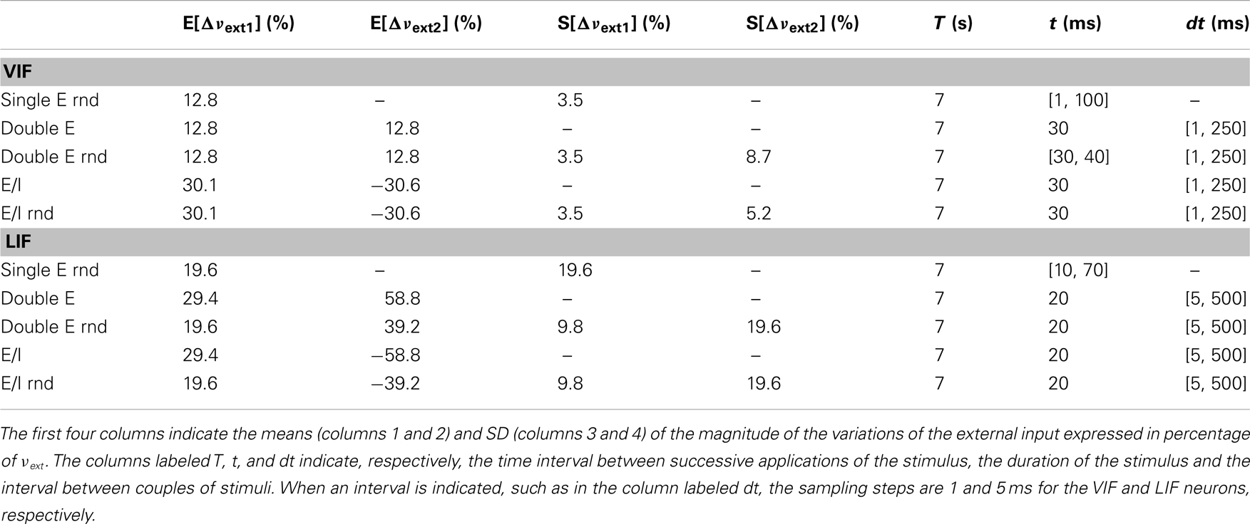
Table A1. Details of the stimulation protocols.