Interareal coupling reduces encoding variability in multi-area models of spatial working memory

Introduction

Persistent spiking activity has been experimentally observed in prefrontal cortex (Funahashi et al., 1989; Miller et al., 1996), parietal cortex (Colby et al., 1996; Pesaran et al., 2002), superior colliculus (Basso and Wurtz, 1997), caudate nucleus (Hikosaka et al., 1989; Levy et al., 1997), and globus pallidus (Mushiake and Strick, 1995; McNab and Klingberg, 2008) during the retention interval of visuospatial working memory tasks. Often, the subject must remember a cue's location for several seconds (Funahashi et al., 1989). Delay period neurons persistently fire in response to a preferred cue orientation as described by a bell-shaped tuning curve. Networks of these neurons, with recurrent excitation between similarly tuned neurons and broadly tuned feedback inhibition, can generate spatially localized “bumps.” The position of these bumps encodes the remembered location of the cue (Compte et al., 2000).

Dynamic variability can degrade the accuracy of working memory over time though. Fluctuations in membrane voltage and synaptic conductance can lead to spontaneous spike or failure events at the edge of the bump, causing the bump to wander diffusively (Compte et al., 2000; Laing and Chow, 2001). Bump attractor networks are particularly prone to such diffusive error because bump positions lie on a line attractor where each location is neutrally stable (Amari, 1977). Interestingly, psychophysical data demonstrates spatial working memory error does scale linearly with delay time, suggesting the underlying process that degrades memory is diffusive (White et al., 1994; Ploner et al., 1998). Much theoretical work has examined network properties that might limit memory degradation. Several computational studies have explored networks built from bistable neuronal units, which sustain persistent states that are less susceptible to noise (Camperi and Wang, 1998; Koulakov et al., 2002; Goldman et al., 2003). In addition, synaptic facilitation has been shown to slow the drift of bump position due to internal variability (Itskov et al., 2011). Synaptic plasticity has also be shown to reduce diffusion of bumps in (Hansel and Mato, 2013). Finally, spatially heterogeneous recurrent excitation can reduce wandering of bumps quantizing the line attractor by stabilizing a finite set of bump locations (Kilpatrick and Ermentrout, 2013; Kilpatrick et al., 2013).

Complementary to these possibilities, we propose that interareal coupling across multiple areas of cortex may reduce error in working memory recall generated by dynamic fluctuations. Multiple representations of spatial working memory have been identified in different cortical areas (Colby et al., 1996). This distributed representation makes working memory information readily available for motor (Owen et al., 1996) and decision-making (Curtis and Lee, 2010) tasks. In addition, this redundancy may serve to reduce degrading effects of noise. It is known that several areas involved in oculomotor delayed response tasks are reciprocally coupled to one another (Constantinidis and Wang, 2004; Curtis, 2006). We presume the representation of a spatial working memory in a single area takes the form of a bump in a recurrently coupled neural field. Projections between areas share information about bump position across the multi-area network. Recently, (Folias and Ermentrout, 2011) showed several novel activity patterns emerge when considering neural fields with multiple areas. In addition, recent analyses of spatiotemporal dynamics of perceptual rivalry have exploited dual population neural field models, where activity in each area represents a single percept (Kilpatrick and Bressloff, 2010; Bressloff and Webber, 2012b). In this study, we focus on activity patterns where bumps in each area have positions that remain close.

Our study mostly focuses on a dual area model of spatial working memory, where each area provides a replicate representation of the presented cue. We begin by demonstrating the neutral stability of the bump position in each area, in the absence of noise and interareal projections. Upon including noise and interareal projections, we use a small-noise expansion to derive an effective stochastic differential equation for the position of the bump in each area. The effective system is a multivariate Ornstein–Uhlenbeck process, which we can analyze using diagonalization. The variance of this stochastic process decreases as the strength of connections between areas increases. Variance reduction relies on cancelations arising due to averaging noise between both areas. Thus, when noise is strongly correlated between areas, the effect of interareal coupling is negligible. Lastly, we show this analysis extends to the case of N (more than two) areas and that for sufficiently strong interareal connections, variance scales as 1/N.

Materials and Methods

Dual Area Model of Spatial Working Memory

We consider a recurrently coupled model commonly used for spatial working memory (Camperi and Wang, 1998; Ermentrout, 1998) and visual processing (Ben-Yishai et al., 1995). GABAergic inhibition (Gupta et al., 2000) typically acts faster than excitatory NMDAR kinetics (Clements et al., 1992), and we assume excitatory synapses contain a mixture of AMPA and NMDA components. Thus, we make the assumption that inhibition is slaved to excitation as in (Amari, 1977). We can then describe average activity u₁(x, t) and u₂(x, t) of neurons in either area by the system (Ben-Yishai et al., 1995; Folias and Ermentrout, 2011; Kilpatrick and Ermentrout, 2013)

$\begin{array}{l}\begin{array}{cc}\begin{array}{l}\tau \text{d}{u}_1(x,t)=\left[-u_1+w_{11}\ast f(u_1)+{\epsilon }^{1/2}{w}_{12}\ast f(u_2)\right]\text{d}t\\ +{\epsilon }^{1/2}\text{d}{W}_1(x,t),\hfill \end{array}& (1\text{a})\end{array}\\ \begin{array}{cc}\begin{array}{l}\tau \text{d}{u}_2(x,t)=\left[-u_2+w_{22}\ast f(u_2)+{\epsilon }^{1/2}{w}_{21}\ast f(u_1)\right]\text{d}t\\ +{\epsilon }^{1/2}\text{d}{W}_2(x,t),\hfill \end{array}& (1\text{b})\end{array}\end{array}$

where the effects of synaptic architecture are described by the convolution

$\begin{array}{cc}{w}_{jk}*f(u_k)={\displaystyle {\int }_{-\pi }^{\pi }{w}_{jk}}(x-y)f(u_k(y,t))\text{d}y,& (2)\end{array}$

for j, k = 1, 2, so the case j = k describes recurrent synaptic connections within a area and j ≠ k describes synaptic connections between areas (interareal). Several fMRI and electrode recordings have revealed correlations between activity in multiple cortical areas during spatial working memory tasks (Constantinidis and Wang, 2004; Curtis, 2006), such as parietal and prefrontal cortex (Chafee and Goldman-Rakic, 1998). However, it seems the strength of these correlations is often not on the order of the activity itself (di Pellegrino and Wise, 1993). For this reason, we presume the strength of interareal connections is weak 0 ≤ ε^1/2 « 1. Note, we could choose to make them a different magnitude than the noise, but for analytical convenience, we choose interareal connection and noise magnitude to be roughly the same. Analysis could still be performed in other cases, but it would simply be more complicated. By setting τ = 1, we can assume that time evolves on units of the excitatory synaptic time constant, which we presume to be roughly 10 ms (Häusser and Roth, 1997). The function w_jk(x − y) describes the strength (amplitude of w_jk) and net polarity (sign of w_jk) of synaptic interactions from neurons with stimulus preference y to those with preference x. Following previous studies, we presume the modulation of the recurrent synaptic strength is given by the cosine

$\begin{array}{cc}{w}_{jj}(x-y)=w(x-y)=\cos (x-y),j=1,2,& (3)\end{array}$

so neurons with similar orientation preference excite one another and those with dissimilar orientation preference disynaptically inhibit one another (Ben-Yishai et al., 1995; Ferster and Miller, 2000). Lateral inhibitory type network architectures are supported by anatomical studies of the delay period neurons in prefrontal cortex (Goldman-Rakic, 1995). Our general analysis will apply to any even symmetric function of the distance x − y, but we typically compute things using (Equation 3) since it eases calculations. Finally, synaptic connections from area k to j are specified by the weight function w_jk(x − y), and we typically take this to be the function

$\begin{array}{cc}{w}_{jk}(x-y)=E_j+M_j\cos (x-y),k\ne j& (4)\end{array}$

where E_j and M_j specify the strength of baseline excitation and modulation projecting to the jth area.

Output firing rates are given by taking the gain function f(u) of the synaptic input, which we usually proscribe to be (Wilson and Cowan, 1973)

$f(u)=\frac{1}{1+{\text{e}}^{\text{−}\gamma (\text{u}\text{−}\theta )}},$

and often take the high gain limit γ → ∞ for analytical convenience, so (Amari, 1977)

$\begin{array}{cc}f(u)=H(u-\theta )=\{\begin{array}{ll}0\hfill & :u<\theta ,\hfill \\ 1\hfill & :u\ge \theta .\hfill \end{array}& (5)\end{array}$

Effects of noise are described by the small amplitude (0 ≤ ε « 1) stochastic processes ε^1/2W_j (x, t) that are white in time and correlated in space so that 〈dW_j(x, t)〉 = 0 and

$\begin{array}{l}\langle \text{d}{W}_j(x,t)\text{d}{W}_j(y,s)\rangle =C_j(x-y)\delta (t-s)\text{d}t\text{d}s,\\ \langle \text{d}{W}_j(x,t)\text{d}{W}_k(y,s)\rangle =C_c(x-y)\delta (t-s)\text{d}t\text{d}s,\end{array}$

describing both local and shared noise in either area, j = 1, 2 with j ≠ k. For simplicity, we assume the local spatial correlations have a cosine profile C_j(x) = c_j cos(x). We also typically assume the correlated noise component has cosine profile so C_c(x) = c_c cos(x). Therefore, in the limit c_c → 0, there are no interareal noise correlations, and in the limit c_c → min (c₁, c₂), noise in each area is maximally correlated. For instance, when c₁ = c₂ = c_c = 1, noise in each area is drawn from the same process.

Multiple-Area Model of Spatial Working Memory

To incorporate the effects of many coupled, redundant areas encoding a spatial working memory, we consider a model with N areas and arbitrary synaptic architecture, given by

$\begin{array}{cc}\begin{array}{l}\tau \text{d}{u}_j(x,t)=\left[-u_j+{\epsilon }^{1/2}{\displaystyle \sum _{k=1}^N{w}_{jk}}*f(u_k)\right]\text{d}t\\ +{\epsilon }^{1/2}\text{d}{W}_j(x,t)\hfill \end{array}& (6)\end{array}$

where u_j represents neural activity in the jth area where j = 1, …, N. As before, we set τ = 1, so each time unit corresponds to the roughly 10 ms timescale of excitatory synaptic conductance. The weight function w_jk(x − y) represents the connection from neurons in area k with cue preference y to neurons in area j with cue preference x as described by (Equation 2). For comparison with numerical simulations, we take weight functions to be the cosines (Equation 3) and (Equation 4) and the firing rate function to be Heaviside (Equation 5). As in the dual area model, noises W_j(x, t) are white in time and correlated in space so that 〈dW_j(x, t)〉 = 0 and

$\langle {\mathrm{dW}}_{\text{j}}(x,t){\text{dW}}_{\text{k}}(y,s)\rangle =C_{jk}(x-y)\delta (t-s)\text{d}t\text{d}s,$

with j, k = 1,…, N, where local noise correlations are described when j = k and noise correlations between areas are described when j ≠ k. For comparison with numerical simulations, we consider C_jj (x) = cos(x) and C_jk (x) = c_c cos(x) for all j ≠ k.

Numerical Simulation of Stochastic Differential Equations

The spatially extended model (Equation 1) was simulated using an Euler–Maruyama method with a timestep 10⁻⁴, using Riemann integration on the convolution term with 2000 spatial grid points. To compute and compare the variances 〈Δ₁(t)²〉 for the dual and multiple area model, we simulated the system 5000 times. The position of the bump Δ_j at each timestep, in each simulation, was determined by the position x in each area j at which the maximal value of u_j(x, t) was attained. The variance was then computed at each timepoint and compared to our asymptotic calculations.

Results

We will now study how interareal architecture affect the dynamics of bumps in multiple area stochastic neural fields. To start, we demonstrate that in the absence of reciprocal connectivity between areas bump attractors exist that are neutrally stable to perturbations that change their position, which has long been known (Amari, 1977; Camperi and Wang, 1998; Ermentrout, 1998). Introducing weak interareal connectivity can decrease the variability in bump position because noise that moves bumps in the opposite direction is canceled due to an attractive force introduced by connectivity. Perturbations that push bumps in the same direction are still integrated, so bumps wander due to dynamic fluctuations, but their effective variance is smaller than it would be without interareal synaptic connections. In the presence of noise correlations between areas, effects of noise cancelation are weaker since stochastic forcing in each area is increasingly similar. Our asymptotic analysis is able to explain all of this with its resulting multivariate Ornstein–Uhlenbeck process.

Bumps in the Noise-Free System

To begin, we seek stationary solutions to Equation (1) in the absence interareal connections and noise (ε → 0). Similar analyses have been carried out for bumps in single area populations (Ermentrout, 1998; Hansel and Sompolinsky, 1998). For this study, we assume recurrent connections are identical in all areas (w_jj = w). Relaxing this assumption slightly does not dramatically alter our results. Note first stationary solutions take the form (u₁(x, t), u₂(x, t)) = (U₁(x), U₂(x)). In the absence of any interareal connections, we would not necessarily expect the peaks of these bumps to be at the same location. However, translation invariance of the system (Equation 1) allows us to set the center of both bumps to be x = 0 to ease calculations. The stationary bump solutions then satisfy the system

$\begin{array}{cc}{U}_1=w*f(U_1),U_2=w*f(U_2),& (7)\end{array}$

so the shape of each bump is only determined by the local connections w. For w given by Equation (3), since U₁(x) and U₂(x) are assumed to be peaked at x = 0, then by also assuming even symmetric solutions, we find

$\begin{array}{cc}\begin{array}{l}{U}_1(x)={\displaystyle {\int }_{-\pi }^{\pi }\cos }yf(U_1(y))\text{d}y\text{cos}x,\\ U_2(x)={\displaystyle {\int }_{-\pi }^{\pi }\cos }yf(U_2(y))\text{d}y\text{cos}x,\end{array}& (8)\end{array}$

where we use cos(x − y) = cosx cosy + sinx siny. We can more easily compute the precise shape of these bumps in case of a Heaviside firing rate function (Equation 5). There is then an identical active region of each bump such that U₁(x) > θ and U₂(x)> θ when x ∈ (−a, a), so the Equation (8) become U₁(x) = U₂(x) = 2sina cosx. Applying self-consistency, U₁(±a) = U₂(±a) = θ, we can generate an implicit equation for the half-widths of the bumps a given by 2sina cosa = sin(2a) = θ. Solving this explicitly for a, we find two solutions on $a\in [0,\pi ]:a_u=\frac{1}{2}{\sin }^{-1}\theta$ and $a_s=\frac{\pi }{2}-\frac{1}{2}{\sin }^{-1}\theta$. Only the bump associated with a_s is stable.

The bumps (Equation 7) are neutrally stable to perturbations in both directions, which can lead to encoding error once the effects of dynamic fluctuations are considered (Kilpatrick et al., 2013). Since the two areas are uncoupled, examining bumps' stability can be reduced to studying each bump's stability individually (see Kilpatrick and Ermentrout, 2013 for details). Translating a bump by a scaling of the spatial derivative U′(x), we find u_j(x, t) = U_j(x) + ε^1/2 U′_j(x) e^λt is associated with a zero eigenvalue (λ = 0), corresponding to neutral stability. To see this, we plug it into the corresponding bump equation of Equation (1) in the absence of noise and interareal connections and examine the linearization

$\begin{array}{cc}\lambda {U^{\prime }}_j(x)=-{U^{\prime }}_j(x)+{\displaystyle {\int }_{-\pi }^{\pi }w}(x-y)f^{\prime }(U_j(y)){U^{\prime }}_j(y)\text{d}y.& (9)\end{array}$

Note, in the limit of infinite gain γ → ∞, a sigmoid f becomes the Heaviside (Equation 5), and

$f^{\prime }(U(x))=\frac{\text{d}H(U(x))}{\text{d}U}=\frac{\delta (x-a)}{|U^{\prime }(a)|}+\frac{\delta (x+a)}{|U^{\prime }(a)|},$

in the sense of the distributions. Equation (9) still hold in this case. Differentiating (Equation 7), and integrating by parts, we find

$\begin{array}{l}-U^{\prime }{}_1+w*[f^{\prime }(U_1)U^{\prime }{}_1]=0,\\ -U^{\prime }{}_2+w*[f^{\prime }(U_2)U^{\prime }{}_2]=0,& (10)\end{array}$

where the boundary terms vanish due to periodicity of the domain [−π, π]. Thus, the right hand side of Equation (9) vanishes, and λ = 0 is the only eigenvalue corresponding to translating perturbations. Thus, either bump (in area 1 or 2) is neutrally stable to perturbations that shifts its position in either direction (rightwards or leftwards), since the bump in each area experiences no force from the other bump.

This changes when we consider the effect of interareal connectivity. Once the two areas of Equation (1) are reciprocally coupled, bumps are stable to perturbations that translate them in opposite directions of one another (see Figure 1). Interareal connections act as a restoring force between the two positions of each bump. We will demonstrate this in the subsequent section by deriving a linear stochastic system for the position of either bump in the presence of small noise and weak interareal connectivity. The restorative nature of interareal connectivity is revealed by the negative eigenvalue associated with the interaction matrix (Equation 15) of our stochastic system, as shown in Equation (18).

FIGURE 1

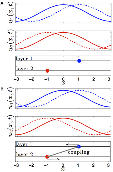
Figure 1. Effect of interareal coupling on the stability of bumps to translating perturbations. (A) In the absence of interareal coupling, bumps (solid) are neutrally stable to perturbations (dashed) that translate them in opposite directions. (B) In the presence of interareal coupling, bumps are linearly stable, as revealed by the negative eigenvalue in Equation (18), to perturbations that translate them in opposite directions.

Noise-Induced Wandering of Bumps

Now we consider the effects of small noise on the position of bumps in the presence of weak interareal connections. We start by presuming noise generates two distinct effects in the bumps (see Figure 2). First, noise causes both bumps to wander away from their initial positions, while still being pulled back into place by the bump in the other area. Bump position in areas 1 and 2 will be described by the time-varying stochastic variables Δ₁(t) and Δ₂(t). Second, noise causes fluctuations in the shape of both bumps, described by a correction Φ_j. To account for this, we consider the ansatz

$\begin{array}{cc}\begin{array}{l}{u}_1=U_1(x-{\Delta }_1(t))+{\epsilon }^{1/2}{\Phi }_1(x-{\Delta }_1(t),t)+\cdots \\ u_2=U_2(x-{\Delta }_2(t))+{\epsilon }^{1/2}{\Phi }_2(x-{\Delta }_2(t),t)+\cdots \end{array}& (11)\end{array}$

FIGURE 2

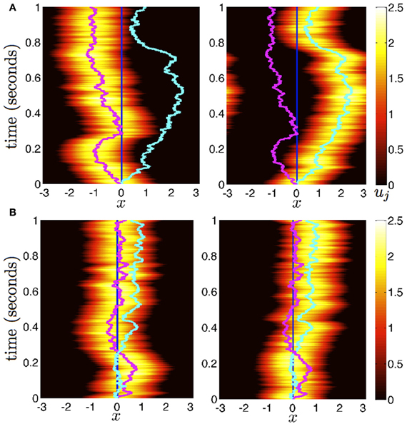
Figure 2. Diffusion of bumps in the dual area stochastic neural field (Equation 1). (A) Without interareal connections (w₁₂ = w₂₁ ≡ 0), each bump executes Brownian motion about the domain, due to stochastic forces. (B) In the presence of interareal connections $\sqrt{\epsilon }{w}_{12}(x)=\sqrt{\epsilon }{w}_{21}(x)\mathrm{=}\mathrm{0.01}(\cos (x)+1)$, the position of bump 1 (magenta) is attracted to the position of bump 2 (cyan) and vice versa. Due to the reversion of each bump to the position of the other, both bumps effectively wander the domain less. Local connectivity is described by the cosine (Equation 3); the firing rate function is Equation (5). Other parameters are threshold θ = 0.5 and noise amplitude ε = 0.025.

Armero et al. (1998) originally developed this approach to analyze of front propagation in stochastic PDE models. In stochastic neural fields, it has been modified to analyze wave propagation (Bressloff and Webber, 2012a) and bump wandering (Kilpatrick and Ermentrout, 2013). Plugging the ansatz (Equation 11) into the system (Equation 1) and expanding in powers of ε^1/2, we find that at (1), we have the bump solution (Equation 7). Proceeding to (ε^1/2), we find

where is the 2 × 1 vector function

Φ = (Φ₁(x, t), Φ₂(x, t))^T; and is the linear operator

for any vector u = (u(x)v(x)^T of integrable functions. Note that the nullspace of includes the vectors (U′₁, 0)^T and (0, U′₂)^T, due to Equation (10). The last terms in the right hand side vector of Equation (12) arise due to interareal connections. We have linearized them under the assumption |Δ₁ − Δ₂| remains small, so

$\begin{array}{l}f(U_j(x+{\Delta }_k-{\Delta }_j))\approx f(U_j(x))\hfill \\ +f^{\prime }(U_j(x))U_j^{\prime }(x)·({\Delta }_k-{\Delta }_j),\hfill \end{array}$

where j = 1, 2 and k ≠ j. To make sure that a solution to Equation (12) exists, we require the right hand side is orthogonal to all elements of the null space of the adjoint , which is defined

for any integrable vector p = (p(x)q(x))^T. It then follows

We can show that the nullspace of contains the vector f₁ = (f′(U₁)U′₁, 0)^T by plugging it into Equation (13) to yield

where 0 = (0, 0)^T and we use Equation (10). We can also show the nullspace of contains f₂ = (0, f′(U₂)U′₂)^T in the same way. Thus, we can ensure Equation (12) has a solution by taking the inner product of both sides of Equation (12) with the two null vectors to yield

$\begin{array}{l}\langle f^{\prime }(U_1){U^{\prime }}_1,{\epsilon }^{-1/2}{\dot{\Delta }}_1{U^{\prime }}_1+\text{d}{W}_1\\ +w_{12}*\left[f(U_2)+f^{\prime }(U_2){U^{\prime }}_2·({\Delta }_2-{\Delta }_1)\right]\text{d}t\rangle =0\\ \langle f^{\prime }(U_2){U^{\prime }}_2,{\epsilon }^{-1/2}{\dot{\Delta }}_2{U^{\prime }}_2+\text{d}{W}_2\\ +w_{21}*\left[f(U_1)+f^{\prime }(U_1){U^{\prime }}_1·({\Delta }_1-{\Delta }_2)\right]\text{d}t\rangle =0,\end{array}$

where we define the inner product 〈u, v〉 = ∫^π_−π u(x)v(x)dx. Therefore, the stochastic vector Δ(t) = (Δ₁(t), Δ₂(t))^T obeys the multivariate Ornstein–Uhlenbeck process

$\begin{array}{cc}\text{d}\Delta (t)\text{=}K\Delta (t)\text{d}t\text{+d}W(t)& (14)\end{array}$

where effects of interareal connections are described by the matrix

$\begin{array}{cc}K=\left(\begin{array}{cc}-{\kappa }_1& {\kappa }_1\\ {\kappa }_2& -{\kappa }_2\end{array}\right),& (15)\end{array}$

with

$\begin{array}{cc}\begin{array}{l}{\kappa }_1=\frac{\langle f^{\prime }(U_1){U^{\prime }}_1,{\epsilon }^{1/2}{w}_{12}*\left[f^{\prime }(U_2){U^{\prime }}_2\right]\rangle }{\langle f^{\prime }(U_1){U^{\prime }}_1,{U^{\prime }}_1\rangle },\\ {\kappa }_2=\frac{\langle f^{\prime }(U_2){U^{\prime }}_2,{\epsilon }^{1/2}{w}_{21}*\left[f^{\prime }(U_1){U^{\prime }}_1\right]\rangle }{\langle f^{\prime }(U_2){U^{\prime }}_2,{U^{\prime }}_2\rangle },\end{array}& (16)\end{array}$

and (w₁₂ * f(U₂)) · U′₁ and (w₂₁ * f(U₁)) · U′₂ vanish upon integration since they are odd. Noise is described by the vector with

The white noise term W has zero mean 〈W(t)〉 = 0 and variance described by pure diffusion so 〈W(t)W^T(t)〉 = Dt with

$\begin{array}{cc}D=\left(\begin{array}{cc}{D}_1& D_c\\ D_c& D_2\end{array}\right)& (17)\end{array}$

where the associated diffusion coefficients of the variance are

$\begin{array}{l}{D}_1=\epsilon \frac{{\displaystyle {\int }_{-\pi }^{\pi }{\displaystyle {\int }_{-\pi }^{\pi }{F}_1}}(x)F_1(y)C_1(x-y)\text{d}x\text{d}y}{\left[{\displaystyle {\int }_{-\pi }^{\pi }{F}_1}(x){U^{\prime }}_1(x)\text{d}x\right]},\\ D_2=\epsilon \frac{{\displaystyle {\int }_{-\pi }^{\pi }{\displaystyle {\int }_{-\pi }^{\pi }{F}_2}}(x)F_2(y)C_2(x-y)\text{d}x\text{d}y}{\left[{\displaystyle {\int }_{-\pi }^{\pi }{F}_2}(x){U^{\prime }}_2(x)\text{d}x\right]}.\end{array}$

where F_j(x) = f′(U_j(x))U′_j(x) and covariance is described by the coefficient

$D_c=\epsilon \frac{{\displaystyle {\int }_{-\pi }^{\pi }{\displaystyle {\int }_{-\pi }^{\pi }{F}_1}}(x)f^{\prime }(U_2(y))F_2(y)C_c(x-y)\text{d}x\text{d}y}{\left[{\displaystyle {\int }_{-\pi }^{\pi }{F}_1}(x){U^{\prime }}_1(x)\text{dx}\right]\left[{\displaystyle {\int }_{-\pi }^{\pi }{F}_2}(x){U^{\prime }}_2(x)\text{dx}\right]}.$

In the next section, we analyze this stochastic system (Equation 14), showing how coupling between areas can reduce the variability of the bump positions Δ₁(t) and Δ₂(t).

Effect of Coupling on Bump Position Variance

To analyze the Ornstein–Uhlenbeck process (Equation 14), we start by diagonalizing the matrix K = V Λ V⁻¹ using the eigenvalue decomposition

$\begin{array}{cc}\begin{array}{l}\Lambda =\left(\begin{array}{cc}0& 0\\ 0& -{\kappa }_1-{\kappa }_2\end{array}\right),\\ V=\frac{1}{{\kappa }_1+{\kappa }_2}\left(\begin{array}{cc}1& {\kappa }_1\\ 1& -{\kappa }_2\end{array}\right),\\ V^{-1}=\left(\begin{array}{cc}{\kappa }_2& {\kappa }_1\\ 1& -1\end{array}\right),\hfill \end{array}& (18)\end{array}$

such that Λ is the diagonal matrix of eigenvalues; columns of V are right eigenvectors; and rows of V⁻¹ are left eigenvectors. Eigenvalues λ₁, λ₂ and eigenvectors v₁, v₂ inform us of the effect of interareal coupling on linear stability. The eigenvalue λ₁ = 0 corresponds to the neutral stability of the positions (Δ₁, Δ₂)^T to translations in the same direction v₁ = (1, 1)^T. The negative eigenvalue λ₂ = − (κ₁ + κ₂) corresponds to the linear stability introduced by interareal connections. The positions (Δ₁, Δ₂)^T revert to one another when perturbations translate them in opposite directions v₂ = (κ₁, −κ₂)^T.

Diagonalizing K = V Λ V⁻¹ using Equation (18), we can compute the mean and variance of the vector Δ(t) given by Equation (14). First, note that the mean 〈Δ(t)〉 = e^Kt Δ(0) (Gardiner, 2003), which we can compute

$\langle \Delta \rangle =\left(\begin{array}{c}({\kappa }_2+{\kappa }_1{\text{e}}^{{\lambda }_{\text{2}}\text{t}}){\Delta }_1(0)+({\kappa }_1-{\kappa }_1{\text{e}}^{{\lambda }_{\text{2}}\text{t}}){\Delta }_2(0)\\ ({\kappa }_2-{\kappa }_2{\text{e}}^{{\lambda }_{\text{2}}\text{t}}){\Delta }_1(0)+({\kappa }_1+{\kappa }_2{\text{e}}^{{\lambda }_{\text{2}}\text{t}}){\Delta }_2(0)\end{array}\right)$

using the diagonalization e^Kt = Ve^Λt V⁻¹. Since λ₂ = −(κ₁ + κ₂) < 0,

$\underset{t\to \infty }{\lim }\langle \Delta (t)\rangle =\left[{\kappa }_2{\Delta }_1(0)+{\kappa }_1{\Delta }_2(0)\right]\left(\begin{array}{c}1\\ 1\end{array}\right).$

Thus, the means of Δ₁(t) and Δ₂(t) always relax to the same position in long time, due to the linear stability introduced by connections between areas. Under the assumption they both begin at Δ₁(0) = Δ₂(0) = 0, the covariance matrix is given (Gardiner, 2003)

$\begin{array}{cc}\langle \Delta (t){\Delta }^T(t)\rangle ={\displaystyle {\int }_{\text{0}}^{\text{t}}{e}^{K(t-s)}}D{\text{e}}^{K^{\text{T}}(\mathrm{t-s})}\text{d}s,& (19)\end{array}$

where D is the covariance coefficient matrix of the white noise vector W(t) given by Equation (17). To compute Equation (19), we additionally need the diagonalization K^T = (V⁻¹)^T Λ V^T, so e^{KT t} = (V⁻¹)^T e^{Λ t} V^T. After multiplying and integrating (Equation 19), we find the elements of the covariance matrix

$\langle \Delta (t){\Delta }^T(t)\rangle =\left(\begin{array}{cc}\langle {\Delta }_1{(t)}^2\rangle & \langle {\Delta }_1(t){\Delta }_2(t)\rangle \\ \langle {\Delta }_1(t){\Delta }_2(t)\rangle & \langle {\Delta }_2{(t)}^2\rangle \end{array}\right)$

are

$\begin{array}{l}\begin{array}{cc}\langle {\Delta }_1{(t)}^2\rangle =D_{+}t+2{\kappa }_1{r}_1(t)+\frac{{\kappa }_1}{{\kappa }_2}{r}_2(t)& (20)\end{array}\\ \begin{array}{cc}\langle {\Delta }_2{(t)}^2\rangle =D_{+}t-2{\kappa }_2{r}_1(t)+\frac{{\kappa }_2}{{\kappa }_1}{r}_2(t)& (21)\end{array}\\ \langle {\Delta }_1(t){\Delta }_2(t)\rangle =D_{+}t+({\kappa }_1-{\kappa }_2)r_1(t)-r_2(t)\hfill \end{array}$

where the effective diffusion coefficients are

$\begin{array}{l}\begin{array}{cc}{D}_{+}=\frac{{\kappa }_2^2{D}_1+2{\kappa }_1{\kappa }_2{D}_c+{\kappa }_1^2{D}_2}{{({\kappa }_1+{\kappa }_2)}^2},& (22)\end{array}\\ \begin{array}{cc}{D}_r=\frac{{\kappa }_2{D}_1-{\kappa }_1{D}_2+({\kappa }_1-{\kappa }_2)D_c}{{({\kappa }_1+{\kappa }_2)}^2},& (23)\end{array}\\ \begin{array}{ll}{D}_{-}=\frac{D_1-2D_c+D_2}{{({\kappa }_1+{\kappa }_2)}^2},& (24)\end{array}\end{array}$

so that D₊ and D₋ are variances of noises occurring along the eigendirections v₁ and v₂. The functions r₁(t), r₂(t) are exponentially saturating

$\begin{array}{l}{r}_1(t)=\frac{D_r}{{\kappa }_1+{\kappa }_2}\left[1-{\text{e}}^{\text{−}({\kappa }_{\text{1}}\text{+}{\kappa }_{\text{2}})\text{t}}\right],\hfill \\ r_2(t)=\frac{{\kappa }_1{\kappa }_2{D}_{-}}{2({\kappa }_1+{\kappa }_2)}\left[1-{\text{e}}^{\text{−2}({\kappa }_{\text{1}}\text{+}{\kappa }_{\text{2}})\text{t}}\right].\end{array}$

The main quantities of interest to us are the variances (Equation 20) and (Equation 21) with which we can make a few observations concerning the effect of interareal connections on the variance of bump positions.

First, note the long term variance of either bump's position Δ₁(t) and Δ₂(t) will be the same, described by the averaged diffusion coefficient D₊, since

$\begin{array}{cc}\underset{t\to \infty }{\lim }\langle {\Delta }_1{(t)}^2\rangle =\underset{t\to \infty }{\lim }\langle {\Delta }_2{(t)}^2\rangle =D_{+}t.& (25)\end{array}$

As the effective coupling strengths κ_j are increased, we can expect the variances 〈Δ_j(t)²〉 approach these limits at faster rates since other portions of the variance decay at a rate proportional to |λ₂| = κ₁ + κ₂.

Next, we study the case, across all times t, where connections between areas are the same (w₁₂ ≡ w₂₁ = w_r) and noise within areas is identical (D₁≡ D₂ = D_l), the mean reversion rates will be the same (κ₁ = κ₂ = κ) and terms in Equation (23) cancel so D_r = 0. Thus, the variances will be identical (〈Δ₁(t)²〉 = 〈Δ₂ (t)²〉 = 〈Δ(t)²〉) and

$\langle \Delta {(t)}^2\rangle =\frac{D_l+D_c}{2}t+\frac{D_l-D_c}{8\kappa }\left[1-{\text{e}}^{\text{−4}\kappa \text{t}}\right].$

This demonstrates the way in which correlated noise (D_c) contributes to the variance. When noise within each area is shared (D_c → D_l), there is no benefit to interareal coupling and 〈Δ(t)²〉 = D_lt (see Kilpatrick and Ermentrout, 2013). However, when any noise is not shared between areas (D_c < D_l), variance can be reduced by increasing coupling strength κ between areas. The variance 〈Δ(t)²〉 is monotone decreasing in κ since

$\frac{\partial }{\partial \kappa }\langle \Delta {(t)}^2\rangle =\frac{D_l-D_c}{8}\frac{(1+4\kappa t){\text{e}}^{-\text{4}\kappa \text{t}}-\text{1}}{{\kappa }^2}\le 0.$

Inequality holds because (1 + 4 κt) ≤ e^{4 κt} is ensured by the Taylor series expansion of e^{4 κt} when κt > 0.

Thus, variance is minimized in the limit

$\begin{array}{cc}\underset{\kappa \to \infty }{\lim }\langle \Delta {(t)}^2\rangle =\frac{D_l+D_c}{2}t.& (26)\end{array}$

Therefore, strengthening interareal connections in both directions reduces the variance in bump position. On the other hand, in the limit of no interareal connections, we find lim_κ→0〈Δ(t)²〉 = D_lt, and the variance in a bump's position is determined entirely by local sources of noise.

Returning to asymmetric connectivity (κ₁ ≠ κ₂), we consider the case of feedforward connectivity from area 1 to 2 (w₁₂≡ 0), κ₁ = 0, so D₊ = D₁ and the formulas for the variances reduce to

$\begin{array}{l}\langle {\Delta }_1{\left(t\right)}^2\rangle =D_{1}t,\\ \langle {\Delta }_2{\left(t\right)}^2\rangle =D_{1}t+\frac{2(D_1-D_c)}{{\kappa }_2}\left[1-{\text{e}}^{-{\kappa }_{\text{2}}\text{t}}\right]\\ +\frac{D_1-2D_c+D_2}{2{\kappa }_2}\left[1-{\text{e}}^{-\text{2}{\kappa }_{\text{2}}\text{t}}\right],\end{array}$

so the pure diffusive term of both variances is wholly determined by the local noise of area 1. Then, only the position of the bump in area 2 possesses additional mean-reverting fluctuations in its position, which arise from local sources of noise that force it away from the position of the bump in area 1. In this situation, the variance of the bump in area 2's position is minimized when

$\underset{{\kappa }_2\to \infty }{\lim }\langle {\Delta }_1{(t)}^2\rangle =\underset{{\kappa }_2\to \infty }{\lim }\langle {\Delta }_2{(t)}^2\rangle =D_{1}t.$

Comparing this with Equation (26) we see that, since D_c ≤ D₁, the variances 〈Δ_j(t)²〉 will always be higher in this case than in the case of very strong reciprocal coupling between both areas. Averaging information and noise between both areas decreases positional variance as opposed to one area simply receiving noise and information from another. Similar results have been recently identified in the context of studying synchrony of reciprocally coupled noisy oscillators (Ly and Ermentrout, 2010).

One important caveat is that if area 1 has more noise than area 2, the weighting of reciprocal connectivity, κ₁ and κ₂, should be balanced to minimize the variance. If the average diffusion coefficient D₊ is weighted too heavily with the area having the larger variance, the area with less intrinsic noise can end up noisier than it would be without reciprocal connectivity. To see this in the extreme case feedforward coupling, note that if D₂ < D₁, then D₂t < D₁t < 〈Δ₂(t)²〉. Thus, the variance of Δ₂(t) increases as opposed to the uncoupled case where 〈Δ₂(t)²〉 = D₂t.

We now derive the optimal weighting of κ₁ and κ₂ to minimize the long term variance (Equation 25) for general asymmetric connectivity, in the absence of correlated noise D_c = 0. To do so, we fix κ₂ and find the κ₁ that minimizes D₊, which happens to be

${\kappa }_1={\kappa }_2\frac{D_1}{D_2}.$

Thus, for identical noise D₁ = D₂, setting κ₁ = κ₂ minimizes D₊. For much stronger noise in area 2 (D₂ » D₁), κ₁ should be made relatively small. In the case of noise correlations between areas (D_c > 0), the optimal value of κ₁ that minimizes (Equation 25) is

${\kappa }_1={\kappa }_2\frac{D_1-D_c}{D_2-D_c}.$

Calculating the Stochastic Motion of Bumps

We now compute the effective variances (Equation 20) and (Equation 21), considering the specific case of Heaviside firing rate functions (Equation 5), cosine synaptic weights (Equation 3) and (Equation 4). Doing so, we can compare our asymptotic results to those computed from numerical simulations. We compute the mean reversion terms κ₁ and κ₂ by noting the spatial derivative of each bump will be U′₁(x) = U′₂(x) = −2 sina sinx and the null vector components are

$f^{\prime }(U_j(x)){U^{\prime }}_j(x)=\delta (x+a)-\delta (x-a).$

for j = 1, 2. Plugging these formulae into Equation (16), we find κ₁ = ε^1/2M₁ and κ₂ = ε^1/2M₂.

We first consider the case of uncorrelated noise between areas, so c_c ≡ 0, meaning D_c = 0. We can compute the diffusion coefficients associated with the local noise in each area assuming cosine spatial correlations

$\begin{array}{cc}{D}_1=\frac{c_1\epsilon }{2+2\sqrt{1-{\theta }^2}},D_2=\frac{c_2\epsilon }{2+2\sqrt{1-{\theta }^2}}.& (27)\end{array}$

We can then compute Equations (20) and (21) directly, for the case of no noise correlations between areas, by plugging in Equation (27).

For symmetric connections between areas, κ = ε^1/2 M₁ = ε^1/2M₂, as well as identical noise, c₁ = c₂ = 1, we have 〈Δ₁(t)²〉 = 〈Δ₂(t)²〉 = 〈Δ(t)²〉 and

$\begin{array}{cc}\langle \Delta {(t)}^2\rangle \text{}=\text{}\frac{\epsilon t}{4(1+\sqrt{1-{\theta }^2})}\text{}+\text{}\frac{\epsilon }{16(1+\sqrt{1-{\theta }^2})\kappa }\left[1-{\text{e}}^{-\text{4}\kappa \text{t}}\right]\text{}.& (28)\end{array}$

We compare the formula (28) to results we obtain from numerical simulations in Figure 3, finding our asymptotic formula (28) matches quite well. In addition, we compare our results for general (possibly asymmetric) reciprocal connectivity to results from numerical simulations in Figure 4. We also show in Figure 5, as predicted, when κ₂ is held fixed, there is a finite optimal value of κ₁ that minimizes variance 〈Δ₁ (t)²〉. Therefore, reciprocal connectivity in multi-area networks should be balanced, in order to minimize positional variance of the stored bump.

FIGURE 3

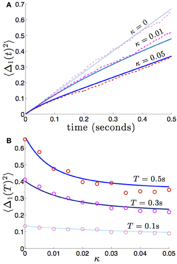
Figure 3. Variance in the position of bumps as computed numerically (red shades) and from theory (blue shades) using Equation (28). Coupling between areas is symmetric $\sqrt{\epsilon }{w}_{12}(x)=\sqrt{\epsilon }{w}_{21}(x)=\kappa (\cos (x)+1)$, so 〈Δ₁(t)²〉 = 〈Δ₂(t)²〉, and there is no shared noise (c_c = 0). (A) The increase in variance is slower for stronger amplitudes of interareal coupling κ. Notice variance climbs sublinearly for κ > 0, due to the mean-reversion caused by coupling. (B) Variance drops considerably more over low values of κ that over high values. Other constituent functions and parameters are the same as in Figure 2.

FIGURE 4

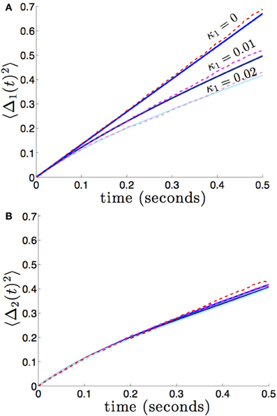
Figure 4. Variance in the position of bumps as it depends on asymmetric reciprocal connectivity (κ₁ ≠ κ₂) when noise in each area is independent and identical (c₁ = c₂ = 1). Fixing κ₂ = 0.02 and varying κ₁, we find (A) the variance 〈Δ₁(t)² of bump 1 decreases as coupling from area 2 to 1 (κ₁) increases; (B) variance 〈Δ₂(t)²〉 of bump 2 remain relatively unchanged. Other constituent functions and parameters are the same as in Figure 2.

FIGURE 5

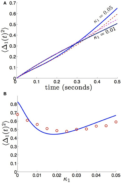
Figure 5. Bump position variance depends non-monotonically on asymmetric connectivity strength. (A) For κ₂ = 0.01 and high enough values of coupling (κ₁ = 0.05), variance 〈Δ₁(t)²〉 scales more quickly than for symmetric coupling (κ₁ = 0.01). Layer 1 is being sourced by the noisier area 2. (B) Non-monotonic dependence of variance 〈Δ₁(t)²〉 on projection strength from area 2 to area 1 κ₁ is shown for fixed time T = 50 and κ₂ = 0.01 fixed. Amplitude of noise in area 2 is twice that of area 1 (c₁ = 1 and c₂ = 2). Other constituent functions and parameters are the same as in Figure 2.

Next, we consider the case of correlated noise between areas, so c_c > 0, meaning D_c > 0. In this case, the covariance terms in D₊ and D₋ are non-zero. We can thus compute the diffusion coefficient associated with correlated noise

$D_c=\frac{c_c\epsilon }{2+2\sqrt{1-{\theta }^2}}.$

In the case of symmetric connections between areas, κ = ε^1/2M₁ = ε^1/2M₂, and identical internal noise, c₁ = c₂ = 1, we have 〈Δ₁(t)²〉 = 〈Δ₂(t)²〉 = 〈Δ(t)²〉 and

$\begin{array}{cc}\langle \Delta {(t)}^2\rangle =\frac{(1+c_c)\epsilon }{4\left(1+\sqrt{1-{\theta }^2}\right)}t+\frac{(1-c_c)\epsilon }{16\left(1+\sqrt{1-{\theta }^2}\right)\kappa }\left[1-{\text{e}}^{-\text{4}\kappa \text{t}}\right],& (29)\end{array}$

which reflects the fact that interareal connections do not reduce variability as much when there are strong noise correlations c_c between areas. We demonstrate the accuracy of the theoretical calculation (Equation 29) as compared to numerical simulations in Figure 6. Numerical simulations also reveal the fact that stronger noise correlations between areas diminish the effectiveness of interareal connections at reducing bump position variance.

FIGURE 6

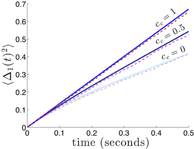
Figure 6. Variance in the position of bumps as noise correlation between areas is increased. Numerically computed variance (red shades) match theoretical curves from Equation (29), blue shades, very well. Reciprocal connectivity reduces variability the most when there is no correlated noise (c_c = 0) between areas. As the shared noise between areas increased is amplitude (c_c = 0.5, 1), the advantage of reciprocal connectivity is diminished. When c_c = 1 changing κ does not affect the variance 〈Δ(t)²〉 (see formula (29) in the limit c_c → 1). Other constituent functions and parameters are the same as in Figure 2.

Reduction of Bump Wandering in Multiple Areas

We now examine the effect of interareal connections in networks with more than two areas using the system (Equation 6). As with the dual area network without noise or interareal connectivity, stationary bump solutions take the form (u₁, …, u_N) = (U₁(x),…, U_N(x)), and translation invariance let us to set all bump peaks to be located at x = 0 so

$\begin{array}{cc}{U}_j=w*f(U_j),j=1,\dots ,N.& (30)\end{array}$

As before, we presume w_jj = w, and relaxing this assumption does not dramatically alter our results. Linear stability analysis of bumps proceeds along similar lines to the dual area network, so we omit those calculations and summarize the results. In the absence of interareal connections, each bump is neutrally stable to perturbation in either direction. In the presence of interareal connections, all bumps are only neutrally stable to translations that move them all in the same direction. Therefore, networks with more areas provide more perturbation cancelations.

To study how noise and interareal connections affect the trajectory of bump positions, we again note noise causes all bumps to wander away from their initial position, while being pulled back into place by projections from other areas (see Figure 7). The position of the bump in area j is described by the stochastic variable Δ_j. Noise also causes fluctuations in the shape of both bumps, which is described by the correction term Φ_j. Therefore, we presume the resulting state of the system satisfies the ansatz

$u_j=U_j(x-{\Delta }_j(t))+{\epsilon }^{1/2}{\Phi }_j(x-{\Delta }_j(t),t)+\cdots ,$

where j = 1,…, N. Plugging this ansatz into Equation (6) and expanding in powers of ε^1/2, we find that at (1), we simply have the system of Equation (30) for the bump solutions. Proceeding to (ε^1/2), we find

where is an N × 1 vector whose jth entry is

Φ = (Φ₁(x, t), …, Φ_N(x, t))^T; and is the linear operator

for any integrable vector Ψ = (Ψ₁(x),…, Ψ_N(x))^T. The nullspace of is spanned by the vectors (U′₁, 0, …, 0)^T; (0, U′₂, 0, …, 0)^T; …; and (0, …, 0, U′_N)^T, which can be seen by differentiating (Equation 30). The last terms on the right hand side of Equation (31) arise due to interareal connections. We have linearized them under the assumption that |Δ_k − Δ_j| remains small for all j, k. To ensure a solution to Equation (31), we require the right hand side is orthogonal to all elements of the null space of the adjoint operator . The adjoint is defined with respect to the inner product

where ϒ = (ϒ₁(x),…,ϒ_N(x))^T is integrable. It then follows

FIGURE 7

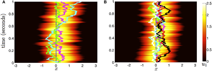
Figure 7. Stochastic evolution of bump position in multi-area networks. (A) With weak coupling $\sqrt{\epsilon }{w}_{jk}(x)=0.01(\cos (x)+1)$ for j ≠ k) between N = 3 areas, the position of bumps 1 (magenta), 2 (cyan), and 3 (green) reverts to one another. We show only the evolution of activity u(x, t) in area 1. (B) For N = 6 areas and the same interareal coupling, the reduction in bump wandering is even more considerable. The trajectories of bumps in all areas (colored lines) stay close together. All other parameters are as in Figure 2.

The nullspace of contains the vectors (f′(U₁)U′₁, 0, …, 0)^T; (0, f′(U₂)U′₂, 0, … 0)^T; …; and (0, …, 0, f′(U_N)U_N′), which can be shown by applying to them and using the formula generated by differentiating (Equation 30). Thus, to be sure (Equation 31) has a solution, we take the inner product of both sides of the equation with all N null vectors and isolate dΔ_j terms to yield the multivariate Ornstein–Uhlenbeck process

$\begin{array}{cc}\text{d}\Delta (t)\text{=}K\Delta (t)\text{d}t\text{+}\text{d}W(t),& (32)\end{array}$

where effects of interareal connections are described by the matrix K ∈ ℝ^N×N where the diagonal and off-diagonal entries are given

$K_{jj}=-{\displaystyle \sum _{k\ne j}{\kappa }_{jk}},K_{jk}={\kappa }_{jk}$

for j = 1,…, N and k ≠ j, where

${\kappa }_{jk}=\frac{\langle f^{\prime }(U_j){U^{\prime }}_j,{\epsilon }^{1/2}{w}_{jk}*[f^{\prime }(U_k){U^{\prime }}_k]\rangle }{\langle f^{\prime }(U_j){U^{\prime }}_j,{U^{\prime }}_j\rangle },$

and we have used the fact that w_jk * f(U_k) · U′_j is an odd function for all j, k, so they vanish on integration. Stochastic forces are described by the vector

The white noise vector W(t) has zero mean 〈W(t)〉 = 0, and covariance matrix 〈W(t)W^T(t)〉 = Dt where associated coefficients of the matrix D are

$D_{jj}=\epsilon \frac{{\displaystyle {\int }_{-\pi }^{\pi }{\displaystyle {\int }_{-\pi }^{\pi }{F}_j}}(x)F_j(y)C_j(x-y)\text{d}x\text{d}y}{{\left[{\displaystyle {\int }_{-\pi }^{\pi }{F}_j}(x){U^{\prime }}_j(x)\text{d}x\right]}^2}.$

where F_j(x) = f′(U_j(x))U′_j(x), which describe the variance within an area and

$D_{jk}=\epsilon \frac{{\displaystyle {\int }_{-\pi }^{\pi }{\displaystyle {\int }_{-\pi }^{\pi }{F}_j}}(x)F_k(y)C_{jk}(x-y)\text{d}x\text{d}y}{\left[{\displaystyle {\int }_{-\pi }^{\pi }{F}_j}(x){U^{\prime }}_j(x)\text{d}x\right]\left[{\displaystyle {\int }_{-\pi }^{\pi }{F}_k}(x){U^{\prime }}_k(x)\text{d}x\right]},$

which describes covariance between areas. Since correlations are symmetric C_jk(x) = C_kj(x) for all j, k, then D_jk = D_kj for all j, k.

A detailed analysis of the linear stochastic system (Equation 32) is difficult without some knowledge of the entries κ_jk. However, we can make a few general statements. We note that all eigenvalues of K must have negative real part or be zero, due to the Gerschgorin circle theorem (Feingold and Varga, 1962), which states that all eigenvalues a matrix K must lie in one of the disks with center K_jj and radius ∑_k≠j |K_jk|. Since K_jj = − ∑_k≠j κ_jk and K_jk = κ_jk, then

$\begin{array}{cc}{K}_{jj}+{\displaystyle \sum _{k\ne j}{K}_{jk}}=-{\displaystyle \sum _{k\ne j}{\kappa }_{jk}}+{\displaystyle \sum _{k\ne j}\left|{\kappa }_{jk}\right|}=0& (33)\end{array}$

is the maximal possible eigenvalue, since κ_jk ≥ 0 for all j, k. Therefore, we expect N eigenpairs λ_j, v_k associated with K, where λ_N ≤ λ_{N − 1} ≤ … ≤ λ₂ ≤ λ₁ = 0. This means we can perform the diagonalization K = V Λ V⁻¹, where Λ is the diagonal matrix of eigenvalues; columns of V are right eigenvectors; and rows of V⁻¹ are left eigenvectors. Therefore, we can decompose the stochastic solution to Equation (32), when Δ(0) = 0 as

$\Delta (t)={\displaystyle {\int }_0^t{e}^{K(t-s)}}\text{d}W(s)={\displaystyle {\int }_0^{t}V}{\text{e}}^{\Lambda (\mathrm{t-s})}{V}^{\text{−1}}\text{d}W(s),$

Thus, as we expect, any stochastic fluctuations in Equation (32) will be integrated or decay over time due to the exponential filters e^{λ_j(t − s)}. In addition, when Δ(0) = 0 the covariance matrix can be computed as

$\begin{array}{cc}\langle \Delta (t){\Delta }^T(t)\rangle ={\displaystyle {\int }_{\text{0}}^{\text{t}}{e}^{K(t-s)}}D{\text{e}}^{K^T(t-s)}\text{d}s,& (34)\end{array}$

where D is the matrix of diffusion coefficients for the covariance 〈W(t) W^T(t)〉. We now compute the covariance in the specific case of symmetric connectivity.

In the case of symmetric connectivity between areas, w_jk = w_r for all j ≠ k, so κ_jk = κ for all j ≠ k. Effects of connectivity between areas are described by the symmetric matrix

$K=\kappa J_N-N\kappa I$

where J_N is the N × N matrix of ones and I is the identity. The eigenvalues of J_N are N, with multiplicity one, and zero, with multiplicity N − 1. Thus, the largest eigenvalue of K = κJ_N − N κI is λ₁ = 0 with associated eigenvector v₁ = (1,…, 1)^T. All other eigenvalues are λ_j = −Nκ for j ≥ 2, with associated eigenvectors v_j = e₁ − e_j, where j = 2, …, N and e_j is the unit vector with a one in the jth row and zeros elsewhere. Our diagonalization of the symmetric matrix K = K^T = V Λ V⁻¹ then involves the diagonal matrix Λ of eigenvalues λ_j; the symmetric matrix V whose columns v_j are right eigenvectors; and the symmetric matrix V⁻¹ whose rows are left eigenvectors. The matrix V⁻¹ takes the form

$V^{-1}=\frac{1}{N}\left(\begin{array}{cccc}1& 1& \cdots & \\ 1& -(N-1)& 1& \cdots \\ & & \ddots & 1\\ 1& \cdots & 1& -(N-1)\end{array}\right).$

We can thus compute the covariance using the diagonalization e^Kt = e^KT_t = V e^Λt V⁻¹. In addition, we will assume each area receives noise with identical statistics (D_jj = D_l) and there are identical noise correlations between areas (D_jk = D_c for j ≠ k), so D = (D_l − D_c)I + D_cJ_N. Multiplying and integrating (Equation 34), we find the diagonal entries (variances) of 〈Δ(t)Δ^T(t)〉 are

$\begin{array}{cc}\langle {\Delta }_j{(t)}^2\rangle =\frac{D_l+(N-1)D_c}{N}t+\frac{(N-1)(D_l-D_c)}{2N^2\kappa }\left[1-{\text{e}}^{-\text{2N}\kappa \text{t}}\right],& (35)\end{array}$

and the off-diagonal entries (true covariances) are

$\langle {\Delta }_j(t){\Delta }_k(t)\rangle =\frac{D_l+(N-1)D_c}{N}t-\frac{(D_l-D_c)}{2N^2\kappa }\left[1-{\text{e}}^{-\text{2N}\kappa \text{t}}\right].$

As revealed by the diffusive term in Equation (35), the system still possesses a rotational symmetry, given by the action of rotating all the bumps in the same direction. Thus, the component of noise in this direction is not damped out by coupling. Thus, note that the long term variance of any bump's position Δ_j(t) will be approximately described by the averaged diffusion

$\underset{t\to \infty }{\lim }\langle {\Delta }_j{(t)}^2\rangle =\frac{D_l+(N-1)D_c}{N}t.$

As the strength of coupling κ or number of areas N is increased, the variances 〈Δ_j(t)²〉 approach this limit at a faster rate, since the other portions of variance decay at a rate proportional to |λ₂| = Nκ. Note also that in the limit D_c → D_l, effects of coupling are negligible and the long term variance of each bump is determined by the diffusion introduced by its area's internal noise.

Returning to study the full variance Equation (35) for symmetric coupling and noise, we make a few observations. First, in the limit of purely correlated noise across areas (D_c → D_l), interareal connections have no effect, and 〈Δ_j(t)²〉 = D_lt for all areas and arbitrary coupling strength. However, if there is any independent noise in each area (D_c < D_l), variance 〈Δ_j(t)²〉 can always be reduced further by increasing coupling strength or the number of areas since

$\frac{\text{d}}{\text{d}\kappa }\langle {\Delta }_j{(t)}^2\rangle =\frac{(N-1)(D_l-D_c)}{2N^2}\times \frac{(1+2N\kappa ){\text{e}}^{-\text{2}N\kappa \text{t}})-\text{1}}{{\kappa }^2}\le 0,$

where inequality (1 + 2Nκt) ≥ e^2Nκt holds due to the Taylor expansion of e^2Nκt when Nκt ≥ 0, and

$\begin{array}{l}\frac{\text{d}}{\text{dN}}\langle {\Delta }_j{\left(t\right)}^2\rangle =-\frac{D_l-D_c}{N^2}\hfill \\ +\frac{D_l-D_c}{2N^3\kappa }\left[2(1+N\kappa t){\text{e}}^{-\text{2}N\kappa t}-N\right]\le 0\end{array}$

when N ≥ 2, since D_l ≥ D_c and due to the Taylor expansion of e^2Nκt. Note, we have temporarily treated N as a continuous variable. Thus, we know the variance 〈Δ_j(t)²〉 to decrease with increasing κ and expect it to decrease with increasing N.

We can compute the variance 〈Δ_j(t)²〉 explicitly in the case of Heaviside firing rate functions (Equation 5), cosine synaptic weights (Equation 3) and (Equation 4). With these assumptions, as well as there being identical noise to all areas (c_jj = 1 for all j, c_jk = c_c for j ≠ k), we find

$D_l=\frac{\epsilon }{2+2\sqrt{1-{\theta }^2}},D_c=\frac{c_c\epsilon }{2+2\sqrt{1-{\theta }^2}},$

so that

$\begin{array}{cc}\langle {\Delta }_j{(t)}^2\rangle =\frac{(1+(N-1)c_c)\epsilon }{2N(1+\sqrt{1-{\theta }^2})}t+\frac{(1-c_c)\epsilon }{4N^2\kappa }\left[1-{\text{e}}^{-\text{2}N\kappa t}\right],& (36)\end{array}$

which reflects the fact that increasing the number of areas will decrease variability, when noise between areas is not too strongly correlated. We demonstrate the accuracy of this formula (36) in Figure 8. In numerical simulations, as predicted by our asymptotic calculations, the variance scales more slowly in time in networks with more areas.

FIGURE 8

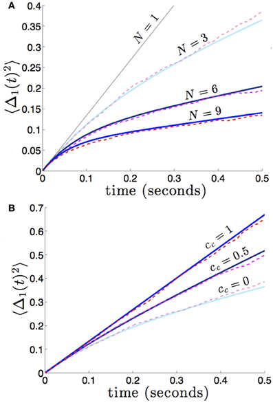
Figure 8. (A) Variance in the position of the bump in the first area 〈Δ₁(t)²〉 builds up more slowly in networks with more areas N, and we expect similar behavior in all other areas. Fixing the strength of interareal connections, $\sqrt{\epsilon }{w}_{jk}(x)=0.01(\cos (x)+1)$ for j ≠ k, we see that varying N decreases the variance 〈Δ_j(t)²〉. (B) As in dual area networks, increasing the level of noise correlations between areas diminishes the effectiveness of interareal connectivity as a noise cancelation mechanism. Other parameters are as in Figure 2.

Discussion

We have shown that interareal coupling in multi-area stochastic networks can reduce the diffusive wandering of bumps. Since bump attractors offer a well studied model of persistent activity underlying spatial working memory (Compte et al., 2000), our results provide a novel suggestion for how the memory networks may reduce error. Our calculations have exploited a small noise approximation for the position of the bump in each area (Armero et al., 1998; Bressloff and Webber, 2012a). Assuming connectivity between areas is weak, we have shown the equations describing bump positions reduce to a multivariate Ornstein–Uhlenbeck process. In this formulation, we find interareal connectivity stabilizes all but one eigendirection in the space of bump position movements. Neutral stability does still exist, so stochastic forces that move bumps in all areas in the same direction do not decay away. However, sources of noise that force bumps in opposite directions create bump movements that will decay with time. Thus, interareal connectivity provides a noise cancelation mechanism that operates by stabilizing the bumps in each area to stochastic forces that push them in opposite directions. (Polk et al., 2012) recently explored noise correlation statistics in persistent state networks that reduce wandering. Our work complements these results by studying synaptic architectures that limit persistent state diffusion.

Storing spatial working memories with neural activity that spans multiple brain areas does serve other purposes than potential noise cancelation. Delayed response tasks that lead to limb motion can generate persistent activity in the parietal cortex (Colby et al., 1996; Pesaran et al., 2002) so that motor responses can be readily executed. In addition, superior colliculus demonstrates sustained activity (Basso and Wurtz, 1997), which is an area also thought to underlie directed behavioral responses. Therefore, activity is distributed between areas providing short term information storage, like prefrontal cortex (Goldman-Rakic, 1995), and those responsible for motor responses and/or behavior. An additional effect of this delegation of activity is that reciprocal connections between areas may provide noise cancelation during the storage period of working memory. However, our work suggests distributing working memory-serving neural activity between areas that receive strongly correlated noise will not provide as effective cancelation.

Our work should be contrasted with several other results concerning the stabilization of networks that encode a continuous variable (Koulakov et al., 2002; Goldman et al., 2003; Cain and Shea-Brown, 2012; Kilpatrick et al., 2013). Pure integrators, which are usually line attractors, are notoriously fragile to parametric perturbations, so (Koulakov et al., 2002) suggested they may be made more robust by considering networks that integrate in discrete bursts, rather than continuously. This can be implemented by considering a population of bistable neural units so that firing rate integration of a stimulus occurs in a stairstep fashion, rather than a ramplike fashion (see Goldman et al., 2003 for example). Related ideas were recently implemented in a bump attractor model of spatial working memory (Kilpatrick et al., 2013), but quantization was implemented with synaptic architecture rather than single neural unit properties. As opposed to the approach of quantizing the space of possible stimulus representations, we have kept the representation space a continuum. Deleterious effects of noise are reduced by considering reciprocal connectivity between encoding areas that redundantly represent the stimulus. Due to noise cancelations, the encoding error of the network decreases as the number of areas is increased.

Conflict of Interest Statement

The author declares that the research was conducted in the absence of any commercial or financial relationships that could be construed as a potential conflict of interest.

References

Amari, S. (1977). Dynamics of pattern formation in lateral-inhibition type neural fields. Biol. Cybern. 27, 77–87. doi: 10.1007/BF00337259

Pubmed Abstract | Pubmed Full Text | CrossRef Full Text

Armero, J., Casademunt, J., Ramirez-Piscina, L., and Sancho, J. M. (1998). Ballistic and diffusive corrections to front propagation in the presence of multiplicative noise. Phys. Rev. E 58, 5494–5500. doi: 10.1103/PhysRevE.58.5494

CrossRef Full Text

Basso, M. A., and Wurtz, R. H. (1997). Modulation of neuronal activity by target uncertainty. Nature 389, 66–69. doi: 10.1038/37975

Pubmed Abstract | Pubmed Full Text | CrossRef Full Text

Ben-Yishai, R., Bar-Or, R. L., and Sompolinsky, H. (1995). Theory of orientation tuning in visual cortex. Proc. Natl. Acad. Sci. U.S.A. 92, 3844–3848. doi: 10.1073/pnas.92.9.3844

Pubmed Abstract | Pubmed Full Text | CrossRef Full Text

Bressloff, P. C., and Webber, M. A. (2012a). Front propagation in stochastic neural fields. SIAM J. Appl. Dyn. Syst. 11, 708–740. doi: 10.1137/110851031

Pubmed Abstract | Pubmed Full Text | CrossRef Full Text

Bressloff, P. C., and Webber, M. A. (2012b). Neural field model of binocular rivalry waves. J. Comput. Neurosci. 32, 233–252. doi: 10.1007/s10827-011-0351-y

Pubmed Abstract | Pubmed Full Text | CrossRef Full Text

Cain, N., and Shea-Brown, E. (2012). Computational models of decision making: integration, stability, and noise. Curr. Opin. Neurobiol. 22, 1047–1053. doi: 10.1016/j.conb.2012.04.013

Pubmed Abstract | Pubmed Full Text | CrossRef Full Text

Camperi, M., and Wang, X. J. (1998). A model of visuospatial working memory in prefrontal cortex: recurrent network and cellular bistability. J. Comput. Neurosci. 5, 383–405. doi: 10.1023/A:1008837311948

Pubmed Abstract | Pubmed Full Text | CrossRef Full Text

Chafee, M. V., and Goldman-Rakic, P. S. (1998). Matching patterns of activity in primate prefrontal area 8a and parietal area 7ip neurons during a spatial working memory task. J. Neurophysiol. 79, 2919–2940.

Pubmed Abstract | Pubmed Full Text

Clements, J. D., Lester, R. A., Tong, G., Jahr, C. E., and Westbrook, G. L. (1992). The time course of glutamate in the synaptic cleft. Science 258, 1498–1501. doi: 10.1126/science.1359647

Pubmed Abstract | Pubmed Full Text | CrossRef Full Text

Colby, C. L., Duhamel, J. R., and Goldberg, M. E. (1996). Visual, presaccadic, and cognitive activation of single neurons in monkey lateral intraparietal area. J. Neurophysiol. 76, 2841–2852.

Pubmed Abstract | Pubmed Full Text

Compte, A., Brunel, N., Goldman-Rakic, P. S., and Wang, X. J. (2000). Synaptic mechanisms and network dynamics underlying spatial working memory in a cortical network model. Cereb. Cortex 10, 910–923. doi: 10.1093/cercor/10.9.910

Pubmed Abstract | Pubmed Full Text | CrossRef Full Text

Constantinidis, C., and Wang, X.-J. (2004). A neural circuit basis for spatial working memory. Neuroscientist 10, 553–565. doi: 10.1177/1073858404268742

Pubmed Abstract | Pubmed Full Text | CrossRef Full Text

Curtis, C. E. (2006). Prefrontal and parietal contributions to spatial working memory. Neuroscience 139, 173–180. doi: 10.1016/j.neuroscience.2005.04.070

Pubmed Abstract | Pubmed Full Text | CrossRef Full Text

Curtis, C. E., and Lee, D. (2010). Beyond working memory: the role of persistent activity in decision making. Trends Cogn. Sci. 14, 216–222. doi: 10.1016/j.tics.2010.03.006

Pubmed Abstract | Pubmed Full Text | CrossRef Full Text

di Pellegrino, G., and Wise, S. P. (1993). Visuospatial versus visuomotor activity in the premotor and prefrontal cortex of a primate. J. Neurosci. 13, 1227–1243.

Pubmed Abstract | Pubmed Full Text

Ermentrout, B. (1998). Neural networks as spatio-temporal pattern-forming systems. Rep. Progress Phys. 61, 353. doi: 10.1088/0034-4885/61/4/002

CrossRef Full Text

Feingold, D. G., and Varga, R. S. (1962). Block diagonally dominant matrices and generalizations of the gerschgorin circle theorem. Pacific J. Math. 12, 1241–1250.

Ferster, D., and Miller, K. D. (2000). Neural mechanisms of orientation selectivity in the visual cortex. Annu. Rev. Neurosci. 23, 441–471. doi: 10.1146/annurev.neuro.23.1.441

Pubmed Abstract | Pubmed Full Text | CrossRef Full Text

Folias, S. E., and Ermentrout, G. B. (2011). New patterns of activity in a pair of interacting excitatory-inhibitory neural fields. Phys. Rev. Lett. 107:228103. doi: 10.1103/PhysRevLett.107.228103

Pubmed Abstract | Pubmed Full Text | CrossRef Full Text

Funahashi, S., Bruce, C. J., and Goldman-Rakic, P. S. (1989). Mnemonic coding of visual space in the monkey's dorsolateral prefrontal cortex. J. Neurophysiol. 61, 331–349.

Pubmed Abstract | Pubmed Full Text

Gardiner, C. W. (2003). Handbook of Stochastic Methods. New York, NY: Springer.

Goldman, M. S., Levine, J. H., Major, G., Tank, D. W., and Seung, H. S. (2003). Robust persistent neural activity in a model integrator with multiple hysteretic dendrites per neuron. Cereb. Cortex 13, 1185–1195. doi: 10.1093/cercor/bhg095

Pubmed Abstract | Pubmed Full Text | CrossRef Full Text

Goldman-Rakic, P. S. (1995). Cellular basis of working memory. Neuron 14, 477–485. doi: 10.1016/0896-6273(95)90304-6

Pubmed Abstract | Pubmed Full Text | CrossRef Full Text

Gupta, A., Wang, Y., and Markram, H. (2000). Organizing principles for a diversity of gabaergic interneurons and synapses in the neocortex. Science 287, 273–278. doi: 10.1126/science.287.5451.273

Pubmed Abstract | Pubmed Full Text | CrossRef Full Text

Hansel, D., and Mato, G. (2013). Short-term plasticity explains irregular persistent activity in working memory tasks. J. Neurosci. 33, 133–149. doi: 10.1523/JNEUROSCI.3455-12.2013

Pubmed Abstract | Pubmed Full Text | CrossRef Full Text

Hansel, D., and Sompolinsky, H. (1998). “Modeling feature selectivity in local cortical circuits,” in Methods in Neuronal Modeling: From Ions to Networks, chapter 13, eds C. Koch, and I. Segev (Cambridge: MIT), 499–567.

Häusser, M., and Roth, A. (1997). Estimating the time course of the excitatory synaptic conductance in neocortical pyramidal cells using a novel voltage jump method. J. Neurosci. 17, 7606–7625.

Pubmed Abstract | Pubmed Full Text

Hikosaka, O., Sakamoto, M., and Usui, S. (1989). Functional properties of monkey caudate neurons. iii. activities related to expectation of target and reward. J. Neurophysiol. 61, 814–832.

Pubmed Abstract | Pubmed Full Text

Itskov, V., Hansel, D., and Tsodyks, M. (2011). Short-term facilitation may stabilize parametric working memory trace. Front. Comput. Neurosci. 5:40. doi: 10.3389/fncom.2011.00040

Pubmed Abstract | Pubmed Full Text | CrossRef Full Text

Kilpatrick, Z. P., and Bressloff, P. C. (2010). Binocular rivalry in a competitive neural network with synaptic depression. SIAM J. Appl. Dyn. Syst. 9, 1303–1347. doi: 10.1137/100788872

CrossRef Full Text

Kilpatrick, Z. P., and Ermentrout, B. (2013). Wandering bumps in stochastic neural fields. SIAM J. Appl. Dyn. Syst. 12, 61–94. doi: 10.1137/120877106

CrossRef Full Text

Kilpatrick, Z. P., Ermentrout, B., and Doiron, B. (2013). Optimizing working memory with spatial heterogeneity of recurrent cortical excitation. (Submitted).

Koulakov, A. A., Raghavachari, S., Kepecs, A., and Lisman, J. E. (2002). Model for a robust neural integrator. Nat. Neurosci. 5, 775–782. doi: 10.1038/nn893

Pubmed Abstract | Pubmed Full Text | CrossRef Full Text

Laing, C. R., and Chow, C. C. (2001). Stationary bumps in networks of spiking neurons. Neural. Comput. 13, 1473–1494. doi: 10.1162/089976601750264974

Pubmed Abstract | Pubmed Full Text | CrossRef Full Text

Levy, R., Friedman, H. R., Davachi, L., and Goldman-Rakic, P. S. (1997). Differential activation of the caudate nucleus in primates performing spatial and nonspatial working memory tasks. J. Neurosci. 17, 3870–3882.

Pubmed Abstract | Pubmed Full Text

Ly, C., and Ermentrout, G. B. (2010). Coupling regularizes individual units in noisy populations. Phys. Rev. E Stat. Nonlin. Soft. Matter. Phys. 81(1 Pt 1):011911. doi: 10.1103/PhysRevE.81.011911

Pubmed Abstract | Pubmed Full Text | CrossRef Full Text

McNab, F., and Klingberg, T. (2008). Prefrontal cortex and basal ganglia control access to working memory. Nat. Neurosci. 11, 103–107. doi: 10.1038/nn2024

Pubmed Abstract | Pubmed Full Text | CrossRef Full Text

Miller, E. K., Erickson, C. A., and Desimone, R. (1996). Neural mechanisms of visual working memory in prefrontal cortex of the macaque. J. Neurosci. 16, 5154–5167.

Pubmed Abstract | Pubmed Full Text

Mushiake, H., and Strick, P. L. (1995). Pallidal neuron activity during sequential arm movements. J. Neurophysiol. 74, 2754–2758.

Pubmed Abstract | Pubmed Full Text

Owen, A. M., Evans, A. C., and Petrides, M. (1996). Evidence for a two-stage model of spatial working memory processing within the lateral frontal cortex: a positron emission tomography study. Cereb. Cortex 6, 31–38. doi: 10.1093/cercor/6.1.31

Pubmed Abstract | Pubmed Full Text | CrossRef Full Text

Pesaran, B., Pezaris, J. S., Sahani, M., Mitra, P. P., and Andersen, R. A. (2002). Temporal structure in neuronal activity during working memory in macaque parietal cortex. Nat. Neurosci. 5, 805–811. doi: 10.1038/nn890

Pubmed Abstract | Pubmed Full Text | CrossRef Full Text

Ploner, C. J., Gaymard, B., Rivaud, S., Agid, Y., and Pierrot-Deseilligny, C. (1998). Temporal limits of spatial working memory in humans. Eur. J. Neurosci. 10, 794–797. doi: 10.1046/j.1460-9568.1998.00101.x

Pubmed Abstract | Pubmed Full Text | CrossRef Full Text

Polk, A., Litwin-Kumar, A., and Doiron, B. (2012). Correlated neural variability in persistent state networks. Proc. Natl. Acad. Sci. U.S.A. 109, 6295–6300. doi: 10.1073/pnas.1121274109

Pubmed Abstract | Pubmed Full Text | CrossRef Full Text

White, J. M., Sparks, D. L., and Stanford, T. R. (1994). Saccades to remembered target locations: an analysis of systematic and variable errors. Vis. Res. 34, 79–92. doi: 10.1016/0042-6989(94)90259-3

Pubmed Abstract | Pubmed Full Text | CrossRef Full Text

Wilson, H. R., and Cowan, J. D. (1973). A mathematical theory of the functional dynamics of cortical and thalamic nervous tissue. Biol. Cybern. 13, 55–80. doi: 10.1007/bf00288786

Pubmed Abstract | Pubmed Full Text | CrossRef Full Text