 Karsten Heusser
 Ramona Heusser2
 Jens Jordan
 André Diedrich
 Jens Tank
- 1Institute of Aerospace Medicine, German Aerospace Center, Cologne, Germany
- 2Immanuel Kant High School, Wilthen, Germany
- 3University of Cologne, Cologne, Germany
- 4Division of Clinical Pharmacology, Department of Medicine, Autonomic Dysfunction Center, Vanderbilt University Medical Center, Nashville, TN, United States
Arterial baroreflex assessment using vasoactive substances enables investigators to collect data pairs over a wide range of blood pressures and reflex reactions. These data pairs relate intervals between heartbeats or sympathetic neural activity to blood pressure values. In an X-Y plot the data points scatter around a sigmoidal curve. After fitting the parameters of a sigmoidal function to the data, the graph’s characteristics represent a rather comprehensive quantitative reflex description. Variants of the 4-parameter Boltzmann sigmoidal equation are widely used for curve fitting. Unfortunately, their ‘slope parameters’ do not correspond to the graph’s actual slope which complicates the analysis and bears the risk of misreporting. We propose a modified Boltzmann sigmoidal function with preserved goodness of fit whose parameters are one-to-one equivalent to the sigmoidal curve’s characteristics.
Introduction
Baroreflexes play an important role in the regulation of the circulatory system. As negative feedback systems they stabilize arterial pressure around the so-called operating pressure. This feature is also known as blood pressure buffering to prevent large deviations from its setpoint. Often cardiovascular diseases are associated with impaired baroreflexes. Therefore, baroreflex quantification may be useful to assess the current state, progression, and therapeutic improvements of cardiovascular diseases. Moreover, precise baroreflex measurements can help unravel complex physiologic or pharmacologic mechanisms (Heusser et al., 2016).
Although there are numerous methods to evaluate baroreflex function they all share the same basic principle of relating the reflex response (output) to the stimulus intensity (input). Typically, systolic arterial pressure is taken as input and heartbeat interval (RR interval, RRI) as output. The quantitative relationship between these parameters is used to characterize the so-called cardiac or vagal or cardiovagal baroreflex. Baroreflex gain or sensitivity is the most reported index. Values range from virtually zero in patients with complete baroreflex failure (Heusser et al., 2005) up to 40 ms/mmHg in trained athletes (Baumert et al., 2006). In cardiovascular laboratories, investigators may be interested in baroreflex mechanisms over a wide range of blood pressures that does not only include the linear part of the stimulus–response relationship but also saturation and threshold portions (Parati et al., 2000). Such data can be obtained by injection or infusion of the vasoactive substances sodium nitroprusside (vasodilator) and phenylephrine (vasoconstrictor). In an X-Y plot, data pairs relating RRI or sympathetic neural activity to blood pressure readings scatter around sigmoidal curves.
Logistic functions (Verhulst, 1838) are widely used for sigmoidal curve fitting, whose prototype was invented to describe population growth with saturation (Figure 1). This function has four characteristic values: Bottom = 0.0, Top = 1.0, and maximum Slope = 0.25 at Midrange = 0.0.
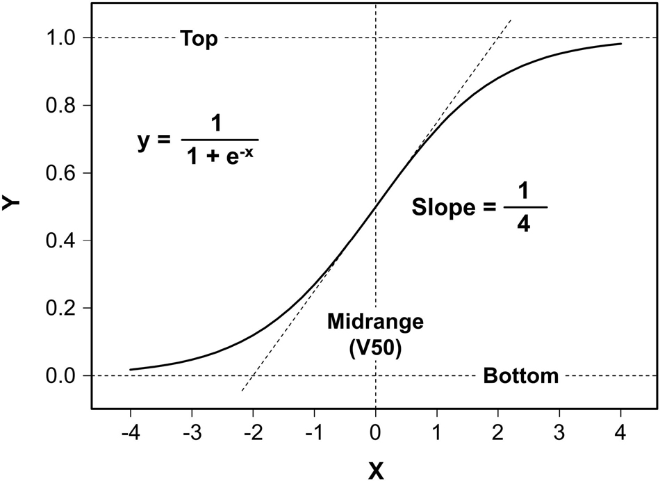
Figure 1. Logistic function. The logistic function (without any parameters) represents the prototype of widely used functions for sigmoidal curve fitting to appropriate classes of two-dimensional experimental data. The graph has four characteristic values: Bottom = 0.0, Top = 1.0, maximum Slope = 0.25 at Midrange = 0.0, which is the abscissa of the curve’s central inflection point.
Most real data that follow a sigmoidal X-Y relationship have other characteristics than the prototypic logistic function. For example, as can be seen from the curve in Figure 2, RR intervals show asymptotic behavior against a lower and upper limit (Bottom and Top) of the baroreflex response which are different from 0.0 and 1.0 of Verhulst’s logistic function. Likewise, the abscissa value of the central inflection point (Midrange) and the slope of the graph at that point (Slope) vary from Verhulst’s values, 0.0 and 0.25, respectively. In 1972, Kent et al. proposed a generalized 4-parameter logistic function, often referred to as Boltzmann sigmoidal equation, to model the baroreflex relationship between systemic arterial and carotid sinus pressure (see Equation 1 in Table 1). Kent et al. used A1..A4 as parameter names. In the following, we will use the more informative terms [B]ottom, [T]op, [R]ange (= T–B), [S]lope, and [M]idrange (or V50). Numerous investigators have applied the equation in its original form or variants thereof for sigmoidal curve fitting to their two-dimensional data (Table 2). The usefulness of the method has been confirmed for decades. It should be particularly emphasized that all 4-parameter equation variants yield absolutely identical output after ideal fitting of the 4 parameters. In other words, after successful fitting of the equations’ parameters to the same data their graphs would perfectly overlap. This statement applies to the traditional equations as well as our modified Equation 8 which will be presented in the Methods section.
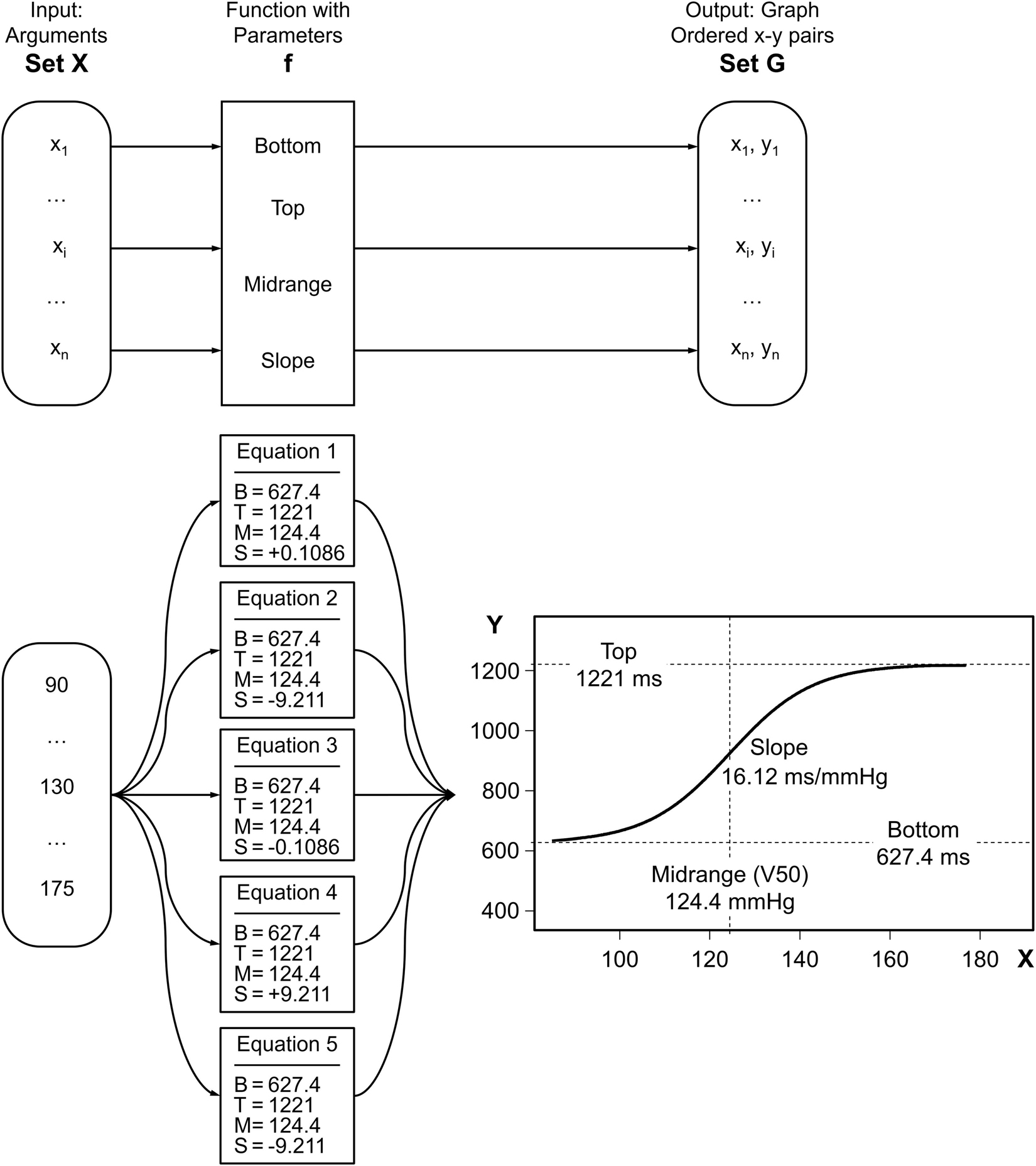
Figure 2. Discrepancy between the equations’ Slope parameters and their graphs’ slopes. The five function boxes in the middle column of the figure implement the versions of the 4-parameter logistic equations in Table 1. The parameters [B]ottom, [T]op, and [M]idrange are identically set for all functions while [S]lope settings differ. However, the functions’ graphs are identical. In other words, the curves representing them are exactly superposed (bottom right). Their identical Slopes at the inflection point at Midrange are 16.12. Hence, there is a discrepancy between [S]lope parameter settings in the functions (middle column) and the functions’ graphs (on the right).
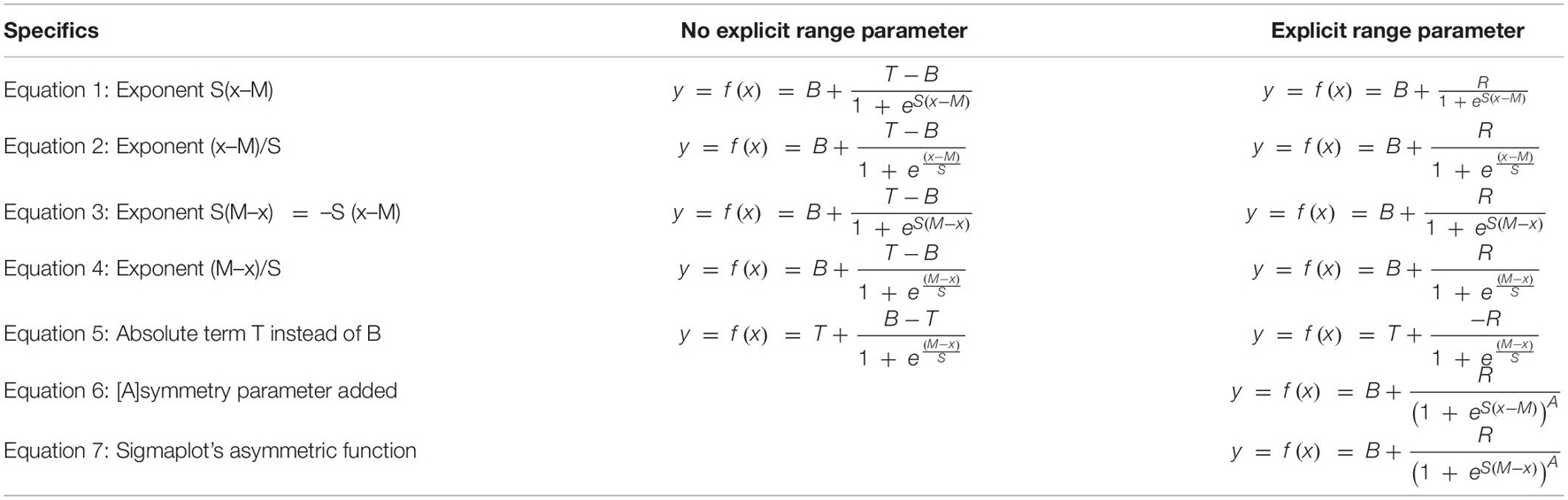
Table 1. Versions of 4- and 5-parameter Boltzmann sigmoidal equations.

Table 2. Selected references referring to variants of the 4-parameter Boltzmann sigmoidal equation.
Ishikawa et al. introduced a fifth parameter (Equation 6) to account for data asymmetry (Ishikawa et al., 1984). According to Ricketts and Head (Ricketts and Head, 1999) Sigmaplot (formerly SPSS now Systat Software Inc.) offers a very similar asymmetric sigmoidal curve fitting equation (Equation 7). The latter authors propose their own asymmetric function (not shown).
The upper part of Figure 2 shows the nomenclature related to functions by taking the example of the Boltzmann sigmoidal function which has 4 parameters (2nd column). The lower part of the figure shows example parameter values that have been obtained by parameter optimization (nonlinear curve fitting) to fit the example data as given in Results section “Curve fitting by means of the modified Boltzmann sigmoidal equation to experimental data.” What all these 5 traditional equations have in common is that their Slope parameters (2nd column) do not represent the slopes of the resultant graphs at their steepest portion at Midrange (see superposed curves in the 3rd column) as naïve users might expect.
The misnomer has several drawbacks. First, there is the risk of using the fitting result ‘as is’ by users who are not aware of the mismatch. Second, users who know about the problem that the parameter represents a surrogate only, called, e.g., “gain coefficient” (do Carmo et al., 2007), “coefficient for the determination of gain” (Scrogin et al., 1994), “slope factor” (Shade et al., 1990), “slope coefficient” (Leitch et al., 1997; Kanbar et al., 2007), “slope parameter” (Devanne et al., 1997), “curvature parameter” (Schenberg et al., 1995), “curvature coefficient” (Cardoso et al., 2005), or “coefficient of curvature” (Leitch et al., 1997), have to determine the true value by further calculation. Third, curve fitting algorithms may need decent starting values or intervals for parameter optimization to successfully converge. Suitable presets for Bottom, Top or Range, and Midrange can be visually derived by the user from X-Y plots of the experimental data. Yet, the Slope parameter as visually estimated from the plots deviates from a useful preset. The latter needs further calculation which complicates the preparation step for curve fitting. Forth, scientific novices cannot readily understand why, after successful curve fitting, three of the four parameter values are equivalent to the graph’s characteristics but Slope (baroreflex gain) is not.
Here we propose a modified Boltzmann sigmoidal equation that ensures one-to-one correspondence between the parameter names and the mathematical characteristics of the resultant graphs. The proposal will simplify sigmoidal curve fitting and, in particular, avoid misinterpretation and misreporting of baroreflex sensitivity.
Methods
Equation 8 is our proposal for a modified Boltzmann sigmoidal equation:
Modified Boltzmann sigmoidal function
Linear form of the equation for usage in fitting tools
The range T–B can be replaced by R. Then, the four parameters would be B, R, M, and S. The formula is not meant to better fit the data; the goodness of fit is exactly the same as for the other 4-parameter variants of the formula (see superposed curves in Figure 2 and report screenshots in Figure 3). Rather, our intention is to reconcile parameter naming and meaning. In the following, we are going to mathematically prove that the four parameters of the modified equation, namely [B]ottom, [T]op, [M]idrange, and [S]lope, exactly reflect the graph’s characteristics. We will do so point by point with the implicit understanding that [S]lope ≠ 0 and [R]ange = [T]op–[B]ottom > 0.0. Normally, the relationship between RR interval and blood pressure has a positive slope. In contrast, the relationships between heart rate or sympathetic nerve activity and blood pressure feature negative slopes.
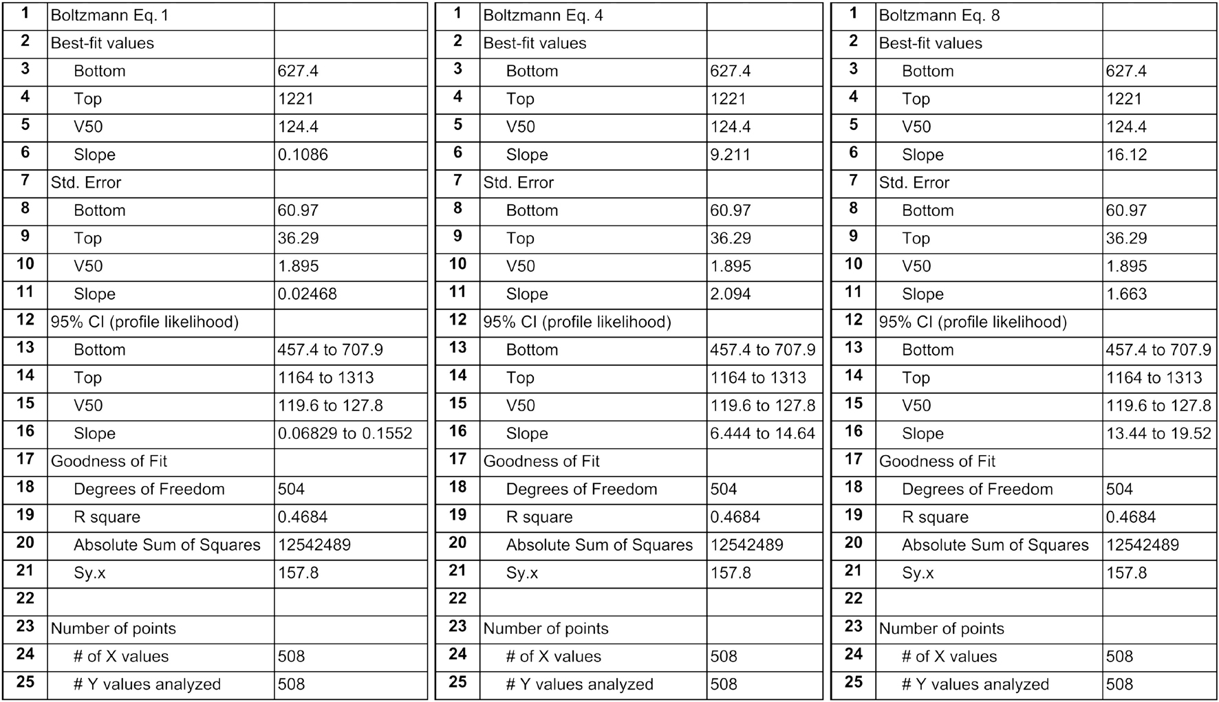
Figure 3. Screenshots of GraphPad® Prism report tables after fitting different Boltzmann sigmoidal functions to real cardiac baroreflex data. We used the nonlinear curve fitting tool of GraphPad Prism (GraphPad, RRID:SCR_002798) to fit the four parameters of the Boltzmann sigmoidal functions related to Equation 1, Equation 4, and Equation 8 to experimentally obtained cardiac baroreflex data from a previous study (Heusser et al., 2016). The result tables report identical values for the optimized parameters Bottom, Top, and Midrange (V50). However, Slopes in line #6 are different. The only Slope that corresponds to the actual slope of the curve (see slope triangle in Figure 4: 16.12 ms/mmHg) is reported by our proposed WYSIWYG Equation 8 as can be expected according to Results section “The [S]lope parameter’s value really represents the slope of the modified Boltzmann sigmoidal curve at the inflection point.” Furthermore, the screenshots exemplify that, after parameter fitting, the resulting graphs are absolutely identical since the Goodness of Fit quantifiers are identical (lines #19–21) which is in agreement with the exactly overlapping curves in Figure 4. Sy.x is a variant of the standard deviation of the residuals that takes the degrees of freedom into account: Sy.x = sqrt [(sum of squared residuals) / (n – degrees of freedom)].
Results
Sections “[B]ottom is the lower limit of the function” through “The [S]lope parameter’s value really represents the slope of the modified Boltzmann sigmoidal curve at the inflection point” prove the correspondence between parameter naming and functional meaning. Captions comment the stepwise proof construction. Section “Threshold and saturation” derives calculation of threshold and saturation pressure. Section “Curve fitting by means of the modified Boltzmann sigmoidal equation to experimental data” exemplifies the usefulness of our proposed equation using real baroreflex data from healthy and diseased subjects, and in section “Practicing curve fitting by means of the modified Boltzmann sigmoidal curve” we invite the readers to test the method on simulated data.
[B]ottom Is the Lower Limit of the Function
With positive slopes the graphs asymptote to [B]ottom toward the left:
(1) S > 0, T–B > 0
a. , x → −∞ ⟹ z → +∞
b.
c.
d.
With negative slopes the graphs asymptote to [B]ottom toward the right:
(2) S < 0, T–B > 0
a. , x → +∞ ⟹ z → +∞
b.
c.
d.
[T]op Is the Upper Limit of the Function
With positive slopes the graphs asymptote to [T]op toward the right:
(3) S > 0, T–B > 0
a. , x → +∞ ⟹ z → −∞
b.
c.
d.
With negative slopes the graphs asymptote to [T]op toward the left:
(4) S < 0, T–B > 0
a. , x → −∞ ⟹ z → −∞
b.
c.
d.
[M]idrange (V50) Is the Abscissa of an Inflection Point
Using the abbreviations
our proposed equation can be written as
To prove the assertion we need the first, second, and third derivatives. They are:
Below we outline that the necessary but not sufficient condition for [M]idrange to be the abscissa of an inflection point of the modified Boltzmann sigmoidal equation, namely f″ (M) = 0, is fulfilled. Note that [M]idrange is passed as x argument to Equation 11:
Given that we disallow [G]radient, which is 4∗[S]lope, to be zero, the sufficient condition for [M]idrange to be the abscissa of an inflection point, namely f‴(M) ≠ 0, is fulfilled, too, as demonstrated below. Note that [M]idrange is passed as x argument to Equation 12:
The Point at x = [M]idrange (V50) Is the Only Inflection Point of the Function
In order for our proposed function to have only one inflection point, f″(x) = 0 must be true for only one x value. To show that this is the case, we reuse Equation 11 while highlighting two crucial terms by enclosing them in curly brackets:
f″ (x) may become zero if at least one of the factors shown in curly brackets above becomes zero.
As ez for all z ∈ ℝ cannot be zero, we have to figure out how to zero the factor on the right:
Calculating the function’s value for x = [M]idrange using Equation 8
shows that it is halfway between the limits [B]ottom and [T]op in analogy to the logistic function prototype whose value is 0.5 at its inflection point (Figure 1).
The [S]lope Parameter’s Value Really Represents the Slope of the Modified Boltzmann Sigmoidal Curve at the Inflection Point
Here we reuse the abbreviations and first derivative as outlined for Equation 9 in section “[M]idrange (V50) is the abscissa of an inflection point”:
and we pass [M]idrange as x argument to the first derivative:
Threshold and Saturation
Midrange is an abscissa-related curve characteristic. In our examples (Figures 2, 4), it is the arterial pressure around which pressure disturbances are effectively buffered by the reflex response. Bottom and Top are distinct ordinate values that represent the upper and lower limits of the reflex response. Abscissa values corresponding to Bottom and Top could indicate the pressure range in which the reflex can operate. Unfortunately, such values do not exist for mathematical reasons, since sigmoidal functions show asymptotic behavior against Bottom and Top. The practical solution was to define Threshold and Saturation as the abscissas, where the sigmoidal curve crosses the 5 and 95% margins of the function’s range (Range = Top – Bottom) (Sabharwal et al., 2004; McDowall and Dampney, 2006). Consequently, the ordinate interval related to Threshold and Saturation covers 90% of the reflex response range (Figure 4). The following derivation is guided by a corrective proposal (McDowall and Dampney, 2006).
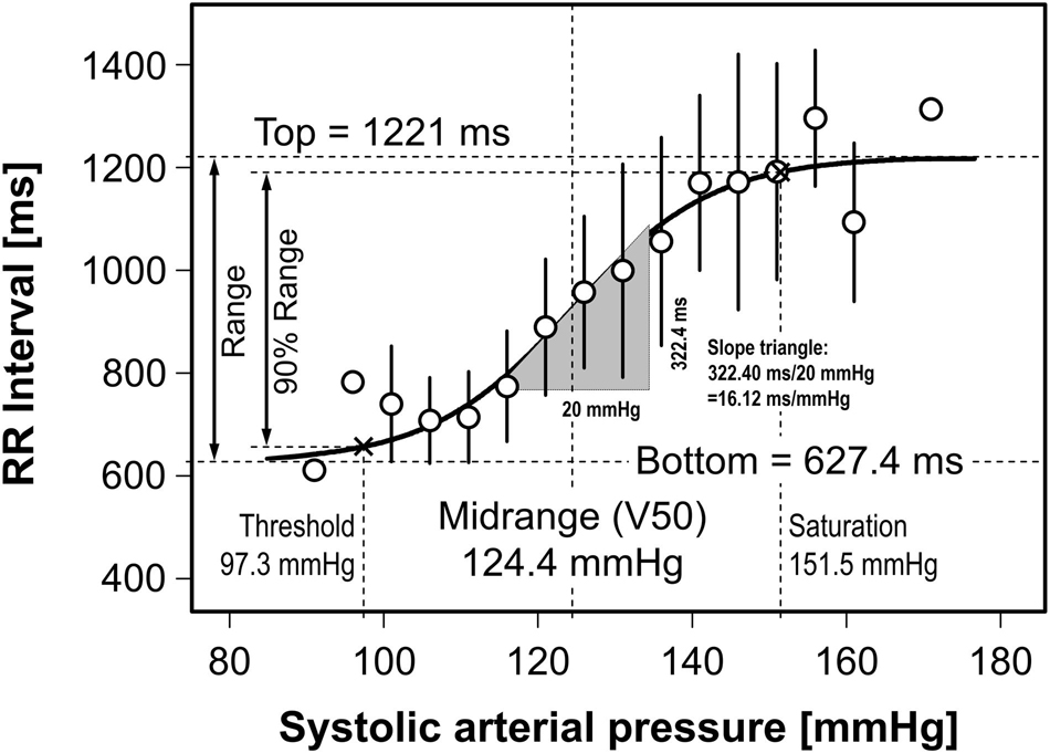
Figure 4. Fitting different Boltzmann sigmoidal functions to real cardiac baroreflex data. Sigmoidal curve fitting to real data from a previous study (Heusser et al., 2016) and illustration of related terminology. After fitting the four parameters of three different equations to these data the resultant function curves overlap exactly. The slope triangle denotes the maximum slopes of the three sigmoidal curves at their inflection point. See Results “Curve fitting by means of the modified Boltzmann sigmoidal equation to experimental data” for more information.
To calculate Threshold and Saturation the first step is to rearrange our proposed Equation 8 to solve for x:
In the second step, we have to pass Bottom + 5% of Range as y argument:
In the third step, we have to pass Bottom + 95% of Range as y argument:
Intermediate steps as above.
Result summary: Threshold and Saturation can be calculated using the formula
Passing the data obtained by curve fitting (Figure 4)
results in Threshold pressure = 97.3 mmHg and Saturation pressure = 151.5 mmHg.
Curve Fitting by Means of the Modified Boltzmann Sigmoidal Equation to Experimental Data
Cardiac baroreflex data have been experimentally obtained earlier in a double-blind, randomized, cross-over study in healthy subjects (Heusser et al., 2016). Stepwise infusions of the vasodilator sodium nitroprusside and the vasoconstrictor phenylephrine elicited blood pressures changes over a large range which is needed for baroreflex curve construction. Comparison of these curves after intake of placebo (see Figure 4) and ivabradine (not shown) challenged the so-called use-dependence of ivabradine and might explain its potential for untoward effects. Such an insight would not have been possible with spontaneous methods for baroreflex quantification.
The data points in Figure 4 relate RR intervals and systolic pressures. They have been binned in 5-mmHg intervals. Bin means are represented as open circles and standard deviations as error bars. Circles related to bins with only one data point lack error bars. Curve fitting procedures were weighted according to the number of data points in each bin. As examples, three variants of the Boltzmann sigmoidal equation, namely Equations 1, 4 and 8 – the latter being our proposal – have been fitted to the data. All three resulting baroreflex curves exactly overlap. Consequently, the goodness of fit (see lines #19–21 in the screenshots in Figure 3) is identical for the three equations. The inserted slope triangle in Figure 4 pertains to the maximum slope of the curves at their central inflection points. The lengths of the triangle’s sides have been chosen for purely graphical reasons. Their ratio of 322.4 ms/20 mmHg = 16.12 ms/mmHg denotes the cardiovagal baroreflex sensitivity (baroreflex gain). In contrast, the Slope parameters reported after curve fitting using traditional versions of the Boltzmann equation (Equation 1: +0.1086 and Equation 4: +9.211) do not correspond to the curve’s actual slope of +16.12 ms/mmHg (line #6 in the screenshots in Figure 3). In contrast, if the modified Boltzmann equation is used all 4 parameter values reflect the graph’s characteristics properly. Hence, only the modified equation features ‘what you see is what you get’ (WYSIWYG).
The modified equation can also be used in patients with disorders of autonomic cardiovascular regulation. The data in Figure 5 represent responses to low-dose injections of sodium nitroprusside (0.25 μg/kg) and phenylephrine (6.25 μg/74 kg) in such a patient. In healthy subjects, these test interventions would hardly change arterial pressure because of the buffering capacity of intact baroreflexes. Yet, in the patient, who also suffers from sympathetic vasoconstrictor incompetence (data not shown), the RR-interval response range is less than 100 ms despite a provoked change in systolic pressure of more than 100 mmHg. Moreover, the baroreflex gain (2.41 ms/mmHg) is much smaller than in healthy subjects. The gray data in Figure 5 are scaled as in Figure 4 for easy visual comparison.
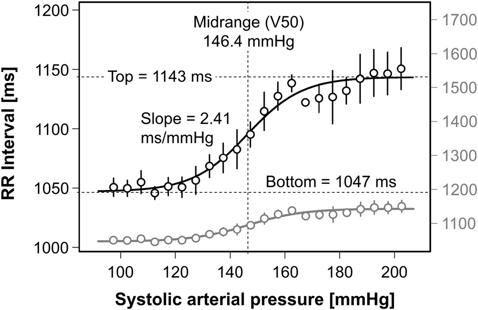
Figure 5. Cardiac baroreflex curve in dysautonomia with marked reductions in response range and baroreflex sensitivity. Sigmoidal curve fitting using Equation 8 has been applied to real data from a patient with dysautonomia. The lower representation of the same data and fitting curve (gray) allows for visual comparison between healthy and diseased subjects because the resolution of the related ordinate on the right (gray) is similar to that in Figure 4. Note the marked reduction in response range (<100 ms) and baroreflex gain (2.41 ms/mmHg).
Practicing Curve Fitting by Means of the Modified Boltzmann Sigmoidal Curve
Interested readers are referred to the Microsoft Excel spreadsheet in the Supplementary Material. The spreadsheet generates two-dimensional data (blood pressure + RR intervals) with adjustable noise. Equation 4 and Equation 8 have been chosen for sigmoidal curve fitting by means of the Excel Solver Add-in. We also suggest to imitate the solver’s attempts to find a good fit by manual adjustments of the equation parameters. By doing so, the reader will realize that adjustments are more direct and easier to achieve when the modified Boltzmann equation is used.
Discussion
Boltzmann sigmoidal equations are frequently used for nonlinear curve fitting to two-dimensional data. Their usefulness has been confirmed for decades. Commonly used forms of the equation have 4 parameters that represent the lower and upper limit or range of the data, the abscissa of the inflection point, and the slope at the latter. They are variants of the formula proposed by Kent et al. (Kent et al., 1972) to provide “a generalized mathematical model of the carotid sinus reflex which contains parameters with meaningful physiological interpretation.” However, while three of the four parameters are directly related to the visible characteristics of the fitting curve, the slope parameter is not. Instead, the actual slope of the curve has to be determined separately. We proposed a modification of the Boltzmann sigmoidal function without this weakness to assist users expecting “what you see is what you get” (WYSIWYG). We mathematically proved that the function’s parameters are one-to-one equivalent to the resultant curve’s characteristics and successfully applied the method to real and artificial baroreflex data. The proposed equation looks slightly more complicated than conventional variants, but it offers some benefits. Once the user has entered the formula in his/her favorite fitting tool, the extra work is loaded onto the computer instead of the user. The traditional mismatch between the slope parameter and the graph’s actual slope is resolved. After the fitting procedure has reached an acceptable result, the reported parameters can be taken as they are computed without any additional postprocessing. The goodness of fit is exactly the same as for the existing variants of the Boltzmann sigmoidal function.
Parameter identifiers like A1..A4 (Kent et al., 1972; Miki et al., 2003; McDowall and Dampney, 2006; do Carmo et al., 2007), P1..P4 (Saad et al., 1989; Itoh and van den Buuse, 1991; Kawada et al., 1992; Bartholomeusz and Widdop, 1995; Sampaio et al., 1999), m1..m4 (Bealer, 2003), a..d (Veelken et al., 1994; He et al., 1999), or a0..a3 (Stewart et al., 2021) are commonly used. More informative names are also assigned to some parameters (Verberne et al., 1987; Schenberg et al., 1995; Cardoso et al., 2005), e.g., BP50, HRmin, and HRmax. The slope parameter, however, continued to be a nomenclatural problem, e.g., “ß is the parameter that governs the slope of the barocurve, i.e., the gain of the baroreflex” (Schenberg et al., 1995) or “dx = a curvature coefficient that is independent of range” (Lee et al., 2002). We hope that our proposal will encourage researchers to embrace meaningful parameter names for sigmoidal curve fitting, including Slope without uncertainty. In our opinion, the more direct identifiers [B]ottom and [T]op as used in Equation 8 should be preferred over [B] and [R]ange, even if we used [R]ange in the Results Section for brevity. In so doing, parameter presetting during the curve fitting preparation step, as often required by fitting tools, is simplified.
Our proposal has the same limitations as the conventional equations. For instance, data asymmetry is not considered (Ishikawa et al., 1984; Ricketts and Head, 1999), and the approach is not able to cope with baroreflex hysteresis (Studinger et al., 2007). The method can only be successfully applied if the blood pressure excursions are large enough to cover the nonlinear parts of the response. Moreover, there is an issue that may occur in vasoactor infusion protocols, namely that the operating pressure after stepwise increasing infusion of sodium nitroprusside may be lower than before. Thus, subsequent infusion of phenylephrine starts from lower pressures than with nitroprusside infusion. This ‘fracture’ in the baroreflex data needs to be handled before curve fitting to prevent slope overestimation. We used Microsoft Excel and the Excel Solver Add-in to illustrate the ideas behind this work using simulated data (see Supplementary Material) because this spreadsheet software is widely known (Microsoft Excel, RRID:SCR_016137). We do not claim particular suitability or superiority over other tools and did not compare curve fitting capabilities of different tools.
Conclusion
Using the proposed WYSIWYG variant of the 4-parameter Boltzmann sigmoidal function for nonlinear curve fitting yields exactly the same results as the traditional ones. In contrast, after successful curve fitting, the resultant value for the Slope parameter can be taken “as is” without any further calculation. Thus, usage of the WYSIWYG equation instead of traditional variants is less time-consuming, cumbersome, and error-prone. The equation has a sound mathematical background which promotes correct physiological interpretation of the results. We encourage the reader to benefit from these advantages.
Data Availability Statement
The original contributions presented in the study are included in the article, further inquiries can be directed to the corresponding author.
Ethics Statement
The studies involving human participants were reviewed and approved by Ethics Committee of Hannover Medical School Study Code CCB-CRC-07-02, Vote #5223NM. The patients/participants provided their written informed consent to participate in this study.
Author Contributions
KH contrived the method and wrote the manuscript draft. RH contrived the mathematical proofs. JJ and JT supplied physiological and clinical background. VU and AD checked maths. All authors contributed to the article and approved the submitted version.
Conflict of Interest
The authors declare that the research was conducted in the absence of any commercial or financial relationships that could be construed as a potential conflict of interest.
Publisher’s Note
All claims expressed in this article are solely those of the authors and do not necessarily represent those of their affiliated organizations, or those of the publisher, the editors and the reviewers. Any product that may be evaluated in this article, or claim that may be made by its manufacturer, is not guaranteed or endorsed by the publisher.
Supplementary Material
The Supplementary Material for this article can be found online at: https://www.frontiersin.org/articles/10.3389/fnins.2021.697582/full#supplementary-material
References
Bartholomeusz, B., and Widdop, R. (1995). Effect of acute and chronic treatment with the angiotensin II subtype 1 receptor antagonist EXP 3174 on baroreflex function in conscious spontaneously hypertensive rats. J. Hypertens. 13, 219–225. doi: 10.1097/00004872-199502000-00009
Baumert, M., Brechtel, L., Lock, J., Hermsdorf, M., Wolff, R., Baier, V., et al. (2006). Heart rate variability, blood pressure variability, and baroreflex sensitivity in overtrained athletes. Clin. J. Sport Med. 16, 412–417. doi: 10.1097/01.jsm.0000244610.34594.07
Bealer, S. L. (2003). Peripheral hyperosmolality reduces cardiac baroreflex sensitivity. Auton. Neurosci. 104, 25–31. doi: 10.1016/S1566-0702(02)00265-5
Cardoso, L. M., Pedrosa, M. L., Silva, M. E., Moraes, M. F. D., and Colombari, E. (2005). Baroreflex function in conscious rats submitted to iron overload. Braz. J. Med. Biol. Res. 38, 205–214. doi: 10.1590/S0100-879X2005000200008
Cheng, Y., Cohen, B., Oréa, V., Barrès, C., and Julien, C. (2004). Baroreflex control of renal sympathetic nerve activity and spontaneous rhythms at Mayer wave’s frequency in rats. Auton. Neurosci. 111, 80–88. doi: 10.1016/j.autneu.2004.02.006
Devanne, H., Lavoie, B., and Capaday, C. (1997). Input-output properties and gain changes in the human corticospinal pathway. Exp. Brain Res. 114, 329–338. doi: 10.1007/PL00005641
do Carmo, J. M., Huber, D. A., Castania, J. A., Fazan, V. P., Fazan, R. Jr., and Salgado, H. C. (2007). Aortic depressor nerve function examined in diabetic rats by means of two different approaches. J. Neurosci. Methods 161, 17–22. doi: 10.1016/j.jneumeth.2006.10.002
Dorward, P. K., Riedel, W., Burke, S. L., Gipps, J., and Korner, P. (1985). The renal sympathetic baroreflex in the rabbit. Arterial and cardiac baroreceptor influences, resetting, and effect of anesthesia. Circ. Res. 57, 618–633. doi: 10.1161/01.RES.57.4.618
He, X.-R., Wang, W., Crofton, J. T., and Share, L. (1999). Effects of 17β-estradiol on the baroreflex control of sympathetic activity in conscious ovariectomized rats. Am. J. Physiol. Regul. Integr. Comp. Physiol. 277, R493–R498. doi: 10.1152/ajpregu.1999.277.2.R493
Heusser, K., Tank, J., Brinkmann, J., Schroeder, C., May, M., Grosshennig, A., et al. (2016). Preserved autonomic cardiovascular regulation with cardiac pacemaker inhibition: a crossover trial using high-fidelity cardiovascular phenotyping. J. Am. Heart Assoc. 5:e002674. doi: 10.1161/JAHA.115.002674
Heusser, K., Tank, J., Luft, F. C., and Jordan, J. (2005). Baroreflex failure. Hypertension 45, 834–839. doi: 10.1161/01.HYP.0000160355.93303.72
Ishikawa, N., Kallman, C. H., and Sagawa, K. (1984). Rabbit carotid sinus reflex under pentobarbital, urethan, and chloralose anesthesia. Am. J. Physiol. Heart Circ. Physiol. 246, H696–H701. doi: 10.1152/ajpheart.1984.246.5.H696
Itoh, S., and van den Buuse, M. (1991). Sensitization of baroreceptor reflex by central endothelin in conscious rats. Am. J. Physiol. Heart Circ. Physiol. 260, H1106–H1112. doi: 10.1152/ajpheart.1991.260.4.H1106
Kanbar, R., Oréa, V., Barres, C., and Julien, C. (2007). Baroreflex control of renal sympathetic nerve activity during air-jet stress in rats. Am. J. Physiol. Regul. Integr. Comp. Physiol. 292, R362–R367. doi: 10.1152/ajpregu.00413.2006
Kawada, T., Fujiki, N., and Hosomi, H. (1992). System analysis of the carotid sinus baroreflex system using a sum-of-sinusoidal input. Jap. J. Physiol. 42, 15–34. doi: 10.2170/jjphysiol.42.15
Kawada, T., Hayama, Y., Nishikawa, T., Yamamoto, H., Tanaka, K., and Sugimachi, M. (2019). Even weak vasoconstriction from rilmenidine can be unmasked in vivo by opening the baroreflex feedback loop. Life Sci. 219, 144–151. doi: 10.1016/j.lfs.2019.01.009
Kent, B. B., Drane, J. W., Blumenstein, B. B., and Manning, J. W. (1972). A mathematical model to assess changes in the baroreceptor reflex. Cardiology 57, 295–310. doi: 10.1159/000169528
Lee, J. S., Morrow, D., Andresen, M. C., and Chang, K. S. (2002). Isoflurane depresses baroreflex control of heart rate in decerebrate rats. J. Am. Soc. Anesthesiol. 96, 1214–1222. doi: 10.1097/00000542-200205000-00026
Leitch, J. W., Newling, R., Nyman, E., Cox, K., and Dear, K. (1997). Limited utility of the phenylephrine-nitroprusside sigmoid curve method of measuring baroreflex function after myocardial infarction. Eur. J. Cardiovasc. Prev. Rehabil. 4, 179–184. doi: 10.1177/174182679700400304
Ma, X., Abboud, F. M., and Chapleau, M. W. (2002). Analysis of afferent, central, and efferent components of the baroreceptor reflex in mice. Am. J. Physiol. Regul. Integr. Comp. Physiol. 283, R1033–R1040. doi: 10.1152/ajpregu.00768.2001
Martel, E., Lacolley, P., Champeroux, P., Brisac, A.-M., Laurent, S., Cuche, J.-L., et al. (1994). Early disturbance of baroreflex control of heart rate after tail suspension in conscious rats. Am. J. Physiol. Heart Circ. Physiol. 267, H2407–H2412. doi: 10.1152/ajpheart.1994.267.6.H2407
McDowall, L. M., and Dampney, R. A. (2006). Calculation of threshold and saturation points of sigmoidal baroreflex function curves. Am. J. Physiol. Heart Circ. Physiol. 291, H2003–H2007. doi: 10.1152/ajpheart.00219.2006
Miki, K., Yoshimoto, M., and Tanimizu, M. (2003). Acute shifts of baroreflex control of renal sympathetic nerve activity induced by treadmill exercise in rats. J. Physiol. 548, 313–322. doi: 10.1113/jphysiol.2002.033050
Mthombeni, N. H., Mpenyana-Monyatsi, L., Onyango, M. S., and Momba, M. N. (2012). Breakthrough analysis for water disinfection using silver nanoparticles coated resin beads in fixed-bed column. J. Hazard. Mater. 217, 133–140. doi: 10.1016/j.jhazmat.2012.03.004
Nagura, S., Sakagami, T., Kakiichi, A., Yoshimoto, M., and Miki, K. (2004). Acute shifts in baroreflex control of renal sympathetic nerve activity induced by REM sleep and grooming in rats. J. Physiol. 558, 975–983. doi: 10.1113/jphysiol.2004.064527
Parati, G., Di Rienzo, M., and Mancia, G. (2000). How to measure baroreflex sensitivity: from the cardiovascular laboratory to daily life. J. Hypertens. 18, 7–19. doi: 10.1097/00004872-200018010-00003
Ricketts, J. H., and Head, G. A. (1999). A five-parameter logistic equation for investigating asymmetry of curvature in baroreflex studies. Am. J. Physiol. Integr. Comp. Physiol. 277, R441–R454. doi: 10.1152/ajpregu.1999.277.2.R441
Rocchiccioli, C., Saad, M., and Elghozi, J.-L. (1989). Attenuation of the baroreceptor reflex by propofol anesthesia in the rat. J. Cardiovasc. Pharmacol. 14, 631–635. doi: 10.1097/00005344-198910000-00015
Saad, M. A., Huerta, F., Trancard, J., and Elghozi, J.-L. (1989). Effects of middle cerebral artery occlusion on baroreceptor reflex control of heart rate in the rat. J. Auton. Nerv. Syst. 27, 165–172. doi: 10.1016/0165-1838(89)90098-2
Sabharwal, R., Coote, J., Johns, E., and Egginton, S. (2004). Effect of hypothermia on baroreflex control of heart rate and renal sympathetic nerve activity in anaesthetized rats. J. Physiol. 557, 247–259. doi: 10.1113/jphysiol.2003.059444
Sagawa, S., Torii, R., Nagaya, K., Wada, F., Endo, Y., and Shiraki, K. (1997). Carotid baroreflex control of heart rate during acute exposure to simulated altitudes of 3,800 m and 4,300 m. Am. J. Physiol. Integr. Comp. Physiol. 273, R1219–R1223. doi: 10.1152/ajpregu.1997.273.4.R1219
Sampaio, K. N., Mauad, H., Biancardi, V. C., Barros, J. L., Amaral, F. T., Schenberg, L. C., et al. (1999). Cardiovascular changes following acute and chronic chemical lesions of the dorsal periaqueductal gray in conscious rats. J. Auton. Nerv. Syst. 76, 99–107. doi: 10.1016/S0165-1838(99)00015-6
Schenberg, L. C., Lucas Brandão, C. A., and Vasquez, E. C. (1995). Role of periaqueductal gray matter in hypertension in spontaneously hypertensive rats. Hypertension 26, 1125–1128. doi: 10.1161/01.HYP.26.6.1125
Scrogin, K. E., Veelken, R., and Luft, F. C. (1994). Sympathetic baroreceptor responses after chronic NG-nitro-L-arginine methyl ester treatment in conscious rats. Hypertension 23, 982–986. doi: 10.1161/01.HYP.23.6.982
Shade, R. E., Bishop, V. S., Haywood, J. R., and Hamm, C. K. (1990). Cardiovascular and neuroendocrine responses to baroreceptor denervation in baboons. Am. J. Physiol. Regul. Integr. Comp. Physiol. 258, R930–R938. doi: 10.1152/ajpregu.1990.258.4.R930
Stewart, J. M., Warsy, I. A., Visintainer, P., Terilli, C., and Medow, M. S. (2021). Supine parasympathetic withdrawal and upright sympathetic activation underly abnormalities of the baroreflex in postural tachycardia syndrome: effects of pyridostigmine and digoxin. Hypertension 77, 1234–1244. doi: 10.1161/HYPERTENSIONAHA.120.16113
Studinger, P., Goldstein, R., and Taylor, J. A. (2007). Mechanical and neural contributions to hysteresis in the cardiac vagal limb of the arterial baroreflex. J. Physiol. 583, 1041–1048. doi: 10.1113/jphysiol.2007.139204
Veelken, R., Hilgers, K. F., Ditting, T., Leonard, M., Mann, J., Geiger, H., et al. (1994). Impaired cardiovascular reflexes precede deoxycorticosterone acetate-salt hypertension. Hypertension 24, 564–570. doi: 10.1161/01.HYP.24.5.564
Verberne, A. J., Lewis, S. J., Worland, P. J., Beart, P. M., Jarrott, B., Christie, M. J., et al. (1987). Medial prefrontal cortical lesions modulate baroreflex sensitivity in the rat. Brain Res. 426, 243–249. doi: 10.1016/0006-8993(87)90878-X
Keywords: baroreflex curve, baroreflex gain, baroreflex sensitivity, RR interval, muscle sympathetic nerve activity, sigmoidal curve fitting, Boltzmann sigmoidal equation
Citation: Heusser K, Heusser R, Jordan J, Urechie V, Diedrich A and Tank J (2021) Baroreflex Curve Fitting Using a WYSIWYG Boltzmann Sigmoidal Equation. Front. Neurosci. 15:697582. doi: 10.3389/fnins.2021.697582
Received: 19 April 2021; Accepted: 31 August 2021;
Published: 27 September 2021.
Edited by:
Alberto Porta, University of Milan, ItalyReviewed by:
Michal Javorka, Comenius University, SlovakiaVlasta Bari, IRCCS Policlinico San Donato, Italy
Teodor Buchner, Warsaw University of Technology, Poland
Copyright © 2021 Heusser, Heusser, Jordan, Urechie, Diedrich and Tank. This is an open-access article distributed under the terms of the Creative Commons Attribution License (CC BY). The use, distribution or reproduction in other forums is permitted, provided the original author(s) and the copyright owner(s) are credited and that the original publication in this journal is cited, in accordance with accepted academic practice. No use, distribution or reproduction is permitted which does not comply with these terms.
*Correspondence: Karsten Heusser, karsten.heusser@dlr.de; orcid.org/0000-0002-2571-5585