Data transfers for nuclear reactor multiphysics studies using the MOOSE framework

High fidelity simulations of nuclear systems generally require a multi-dimensional representation of the system. Advanced nuclear reactor cores are governed by multiple physical phenomena which should be all be resolved, and the coupling of these physics would also need to be resolved spatially in a high-fidelity approach, while lower fidelity may leverage integrated quantities for the coupling instead. Performing a spatially resolved multiphysics simulation can be done on a single mesh with a single coupled numerical system, but this requires catering to each equations’ time and spatial discretization needs. Instead, each physics, usually neutronics, thermal hydraulics and fuel performance, are solved individually with the discretization they require, and the equations are coupled by transferring fields between each solver. In our experience coupling applications within the MOOSE framework, mostly for advanced nuclear reactor analysis, there are several challenges to this approach, from non-conservation problems with dissimilar meshes, to losses in order of spatial accuracy. This paper presents the field transfer capabilities implemented in MOOSE, and numerous technical details such as mapping heuristics, conservation techniques and parallel algorithms. Examples are drawn from nuclear systems analysis cases to illustrate the techniques.

1 Introduction

Modeling and simulation of nuclear reactors is necessary for design, licensing, and operations purposes. The power distribution, the temperature of the fuel, and heat flux-related metrics must be gathered to ensure the nuclear reactor meets safety considerations. For most reactors, obtaining these distributions amounts to solving three groups of equations: neutron transport with depletion and precursors, thermomechanical equations in the solid structures, and thermal-hydraulic equations in the coolant. Over the last 70 years, these equations have been extensively studied and solved for light water reactor analysis. Engineering approximations have been developed and models have been tuned to obtain models that are representative of the reality of their operation. The advent of a new generation of advanced nuclear reactors is challenging these tools, and the plurality of designs rendered in simulations requires a generality the current tools cannot achieve.

This generality is provided by leveraging unstructured mesh to represent these arbitrary geometries. On unstructured meshes, we can deploy finite element (Schoder and Roppert, 2025; Lindsay et al., 2022), finite volume (Schunert et al., 2021), and sweeping methods (Gaston, 2019; Gaston et al., 2021; Prince et al., 2024) to solve equations. Another challenge comes from the wide variety of physics interactions involved in these new reactors, as many of the new designs introduce physics-based passive safety. Modeling different physics in the reactor is relied upon to provide a safe outcome in the case of accidental transients such as reactivity insertion accidents or loss of flow accidents (Forum, 2024). These features can be modeled at various levels of fidelity and complexity for each physics, but there is a constant need to couple different physics solvers.

The United States Department of Energy Nuclear Energy Advanced Modeling and Simulation (NEAMS) program supports the development of a suite of mixed-fidelity simulation tools based on the Multiphysics Object Oriented Simulation Environment (MOOSE) (Lindsay et al., 2022) C++ framework. These include BISON (Williamson et al., 2021) for fuel performance, Griffin (Prince et al., 2024) for neutronics, SAM (Hu et al., 2021) for systems thermal-hydraulics, Pronghorn (Schunert et al., 2021) for multidimensional thermal-hydraulics, and a selection of MOOSE-wrapped codes. MOOSE provides these codes with support for unstructured mesh via an interface to libMesh (Kirk et al., 2006). Unstructured meshes enable the accurate representation of the geometry of these advanced reactors. The shared framework enables an efficient and easy-to-use coupling of the multiple physics, which is the subject of this paper.

About two-thirds of the first three sections of this paper were presented at the Super Computing for Nuclear Applications conference in Paris in October 2024 (Giudicelli et al., 2024a). Additional techniques and figures were added to these sections, the content was re-organized and reworked to improve clarity, and additional examples and results were included in the final section.

2 Coupling simulations with MOOSE-based or wrapped codes

MOOSE was originally designed to attempt to solve every equation in a single Preconditioned Jacobian-Free Newton Krylov method-based solve. With potentially an additive, multiplicative or Schur complement field split, all the equations could be written as a single nonlinear problem. This was successful for a very narrow selection of problems featuring very strong interactions between equations Wang et al. (2017). For most others, differences in required spatial or time discretizations, and in numerical methods to solve equations, rendering this approach inefficient to unworkable.

Hence, this initial approach has been superseded for most advanced reactor simulations with an operator split in which each simulation is performed independently and coupled through fixed point iterations (Gaston et al., 2015). MOOSE greatly simplifies this approach by introducing the MultiApps system. MultiApps are created by a parent application, often in a distributed manner, to nest other physics solves. For example, a Griffin neutronics simulation may spawn BISON MultiApps for each fuel pin calculation. A hierarchy of MultiApps is shown in Figure 1.

Figure 1

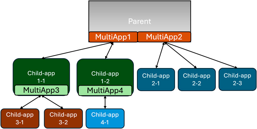
Figure 1. Two-level hierarchy of Multiapps. MultiApps created in the parent app has two independent child applications, each having a MultiApp creating child application(s). The bi-directional arrows represent data transfers between applications.

Once the simulations are created, they can exchange data using the Transfers system. Transfers are created by users to pass fields and scalars between applications. Fields are multi-dimensional, while scalars are typically reductions computed from the fields. They are capable of projecting fields across different meshes, even non-overlapping. Transfers handle the complexities of distributed simulations, for example, if the parent and child application(s) use different numbers of processes. Field transfers are described in more detail in Section 3, while scalar transfers are described in Section 4.

An additional point of interest is that MOOSE-based and MOOSE-wrapped applications are easily combined. The build infrastructure makes building applications combining several MOOSE-based or wrapped applications a trivial task. If the codes are not built together, an application can still be dynamically loaded by another at runtime. The user may specify in the input the application type for the MultiApp and the dynamic library to load to create this application.

2.1 Parallel execution of MultiApps

MultiApps are distributed to maximize the utilization of the machine with an equal split distribution of the processes by default among child applications. There are no set limits to the number of processes used. For example, in Figure 1, if the main application is run with 12 processes, then MultiApp1 is first solved with 12 processes split between the two child applications. Then, MultiApp3 is solved with six processes split between the two grandchild applications, while child application four to one is solved with six processes concurrently. Child application 2-1, two to two, and two to three of MultiApp2 are solved with four processes each once MultiApp1 has been run. Child apps within a MultiApps are solved concurrently.

Executing several MultiApps concurrently is not currently possible but is a topic of interest as this would let a CPU-heavy and a GPU/accelerator-heavy MultiApp execute concurrently and make the best use of available resources. This limitation is due to the sequential execution of each MultiApps, and parallelization being only performed over child applications.

2.2 Siblings transfers

A recent improvement of the Transfer system is the development of child-to-child application transfers, which we refer to in publications related to MOOSE as siblings transfers (Giudicelli et al., 2024b). Previously, MOOSE could only handle transfers between parent and child applications, so transferring between two child applications of different MultiApps would require one transfer from a child to a parent application, and another from the parent to the other child application. Sibling transfers are widely supported across transfers, including all the field transfers mentioned in Sections 3, 4.

An example of these transfers is shown for a molten salt reactor (MSR) core multiphysics case in Figure 2. The neutronics calculation requires the temperature field from the thermal hydraulics calculation, which itself requires the local heat source to solve for the energy conservation equation. The delayed neutron precursor equations requires the velocity fields from thermal hydraulics to solve for their advection, and the fission source from the neutronics to solve for their production. The delayed neutron precursor concentration is then transferred back to the neutronics solver to describe the delayed neutron source, a part of the fission source. The siblings transfer capability enables the leftmost organization of the solves, which does not require the duplication of both fields and transfers in the other schemes. The reader should note that the order of execution of the solvers can be re-arranged. For example, the neutronics could be executed first, then send the power distribution to the thermal hydraulics, then using that velocity field, the precursor advection equations can be solved.

Figure 2

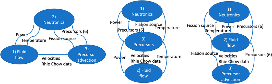
Figure 2. Multiphysics core coupling schemes for a molten salt reactor core analysis case, with sibling transfers (left) enabling a simpler scheme and lower duplication of fields alternative schemes (two alternatives shown on the center and right). The application at the top is the parent and the numbering indicates the order of execution. By default, transfers to an application are executed before this application executes, transfers from an application are executed after this application executes.

Of note, the recent development of multi-system capabilities, solving multiple nonlinear systems on the same mesh, enables defining both fluid flow and precursor advection equations in the same input file. This negates the need for duplicating fields, and thus for siblings transfers for this MSR application.

3 Field-to-field transfers

Transferring a field from a simulation that computes or generates it to a simulation that is influenced by this quantity is a common need. For example, the neutronics solve generates the power density field, which is necessary for the thermal physics solve. Transferring a field between two solves is non trivial. The two solves may be using different meshes, may be partitioned differently in parallel, or may have different finite element representations for the field. We first present the communication algorithm in Subsection 3.1, then the field reconstruction algorithm in 3.2, then the several options for providing source values in 3.3, how to conserve integral quantities in 3.4, how to map regions in 3.5, and finally automated diagnostics to look for ill-posed transfers in 3.7.

3.1 Asynchronous transfer algorithm

The communications required for field transfers between (perhaps distinctly) parallel-distributed mesh data are handled via the asynchronous sparse communication algorithms made available in MOOSE by the Templated Interface to MPI (TIMPI) library. This library provides a wealth of algorithms to perform communication operations between processes, from very simple communicator.gather(vector) operations to the parallel asynchronous push-pull algorithm which we leveraged here.

When each MPI rank has gathered some amount of data to send to some subset of other MPI ranks, in a “sparse push,” for them to act on, a nested map of containers of these data is provided to be sent, and a function object (commonly a C++ lambda) is provided to act on received data. Container data types are used to automatically infer or create a corresponding MPI type (for fixed-size data) or a buffering strategy (for variable-size data), and the API then handles all “sends” and “receives” of data, and calls the provided function object with each received vector. Sends and receives are done asynchronously via the non-blocking exchange (NBX) algorithm, allowing for proper scalability up to large processor counts where the send pattern is typically extremely sparse. For a “sparse pull,” in which data are requested from other processors, a push of request keys (such as mesh indices or geometric locations) is followed by a response push of the requested data values associated with those keys; in this case, the transfer code provides a function object with which to collect data for each request and another function object with which to process the collected and received data.

For field-to-field transfers, the “sparse pull” is used to request data at locations specified by the GenericProjector (see 3.2) to reconstruct the target field. The function to determine which processes may have these data is based on one of three user-selectable heuristics. The first one is the nearest-app heuristic. Only processes working on the child application that is nearest to the needed location are contacted to provide a value. The second one is based on forming a sphere of interest around each target point from the application bounding boxes. The bounding box, possibly inflated or fixed using user parameters, around the domain of each process is checked for every process. We find the minimum of the maximum distances within a bounding box from the point of interest. This creates a sphere around the point of interest. Only processes whose bounding boxes intersect this sphere are contacted to provide a value for this target point. The last one is the greedy search, which is mostly used for debugging. This one requests data from every single other rank, and is therefore not scalable.

3.2 Generic projection capability in the context of asynchronous transfers

The GenericProjector code in libMesh was designed to enable the restriction of arbitrary input functions to arbitrary supported finite element bases. Input functions are defined by the function values they return at arbitrary points and, in cases of higher-continuity finite element spaces, function gradients are either directly provided or inferred by finite differencing. In a typical libMesh use case, the input function is locally evaluable and the projection operation onto a $C_0$-continuous finite element space is thus straightforward: vertex points are first evaluated and directly copied onto vertex degrees of freedom, then quadrature points on element edges are evaluated to enable local $L^2$ projections of element edge values while holding vertex values constant, then (in 3D) element face degrees of freedom are evaluated via projection holding vertex and edge values constant, then finally element interior degrees of freedom are projected while holding each element’s boundary values constant. Each of these local projections is an implicit solve, but with few degrees of freedom, and hence reasonably fast.

In MOOSE, differences between domain and partitioning of transfer source meshes may make it impossible to locally evaluate input functions, so the usage of GenericProjector is slightly more complex. The projection code is evaluated twice: once to determine which quadrature point data will be required from which remote processors, and then a second time to actually evaluate projections and so transfer the data responses correctly to the output field. As with the communications code, the projection code is designed to accept function objects for its innermost operations. The transfer code first provides objects, which merely examine and encapsulate each of the queries to be sent, then provides objects which evaluate cached response data and write projection results to the appropriate field vector coefficients.

3.3 General field transfers

Fields have spatially dependent values on the mesh. Fields in MOOSE are generally variables, though material properties and functions can also be considered fields. There are three main algorithms for performing field transfers in MOOSE. Once the target application has sent its requests for values at certain points, the source application can.

$•$ Evaluate the source variable at the requested points by evaluating the shape functions and performing the finite element reconstruction. This is implemented by the MultiAppGeneralField- ShapeEvaluationTransfer class.

$•$ Return the “nearest” or a combination of the “nearest” values, which are formed at the nearest node or nearest element centroid on which the value of the source variable is known. This avoids evaluating the shape functions. This is implemented by the MultiAppGeneralFieldNearestLocationTransfer class. This class was previously named MultiAppGeneralFieldNearestNodeTransfer and the previous name is still in use.

$•$ Evaluate a source user object at the requested point. This is often to evaluate the source variable through this user object’s operation, for example, layered averaging or other reduction operations. This is implemented by the MultiAppGeneralFieldUserObjectTransfer class.

The implementations of these three algorithms leverage the techniques explained in Sections 3.1, 3.2 through a common base class called MultiAppGeneralFieldTransfer. The derived classes are simply defining how to evaluate the value at a target point, and related details like the detection of ill-posedness. The first two transfer options are also found in other data transfer libraries (Pawlowski et al., 2013), as is the L2-projection transfer which is not described here as it is implemented very differently in MOOSE.

3.4 Conserving integral quantities

An important concern when transferring fields is preserving integral quantities. The most common issue is to preserve power when passing the power distribution from the neutronics solvers to either the fuel performance solver for solid-fueled reactors, or the thermal-hydraulics solver for molten-fuel reactors. For power, the conservation problem is rather simple and only requires a re-scaling by the ratio of integrated power on the source and target meshes. This re-scaling can be distributed if there are multiple target applications, for example, fuel pin solves that have a different local conservation error during the transfer.

At this time, the relation between the field and the postprocessed data is assumed to be linear, so only a single correction step is performed. If the postprocessed data were to be recomputed, we would expect this rescaling to have equalized the ratio between the source and target quantities. However, this would not hold for nonlinear quantities. For example, if the specific heat depends on temperature, rescaling a transferred temperature field once would not suffice to provide conservation of energy.

3.5 Mapping source and origin regions

With the popularity of nearest-node or nearest-element value approaches, a major concern arises in that the nearest-location value is not actually the correct value to obtain. Differences in axial meshes might make the nearest value for the temperature field come from another solid region. For example, for the temperature field where transfers match fuel pins together, an axial mesh cell for a guide-tube in the source application could be closer to the target mesh cell, and therefore would erroneously provide the source value. MOOSE offers a wide variety of region-mapping options to make sure this does not happen.

The simplest options offered are to restrict both source and target domains using block (a subdomain of the mesh) and/or boundary restrictions. These restrictions can be combined completely independently, but the user must understand an important detail. Block and boundary restrictions are restrictions, not matches. Specifying two source blocks and two target blocks does not match the first source block to the first target block. It simply specifies that the transfer will find values from both targets blocks in the union of the two source blocks.

Another restriction technique when using multiple child applications is to use only values from the closest child application to each requested point. This technique is also used as a heuristic to determine which processes should communicate, as mentioned in Subsection 3.1. This technique is particularly useful for consistently matching fuel rods to the channels nearby when using a “nearest-node/location” approach. The concern is that a mismatch between the axial meshes of the rods would map cells in a channel nearest to a certain rod to another rod with a locally finer axial mesh.

To offer a much finer-grained mapping capability, the concept of mesh divisions was introduced. Mesh divisions are an arbitrary indexing of the source and target meshes. The source and target mesh divisions can be matched on a per-index basis. This concept can easily cover the block and boundary restrictions options, but these are kept for backwards compatibility and user friendliness. Example mesh divisions are represented in Figure 3 for various reactor applications: a pin indexing in Figure 3a, a pin and rings indexing in Figure 3b, and a pebble and rings indexing in Figure 3c. Numbering these regions enables focused transfers between physics solvers.

Figure 3

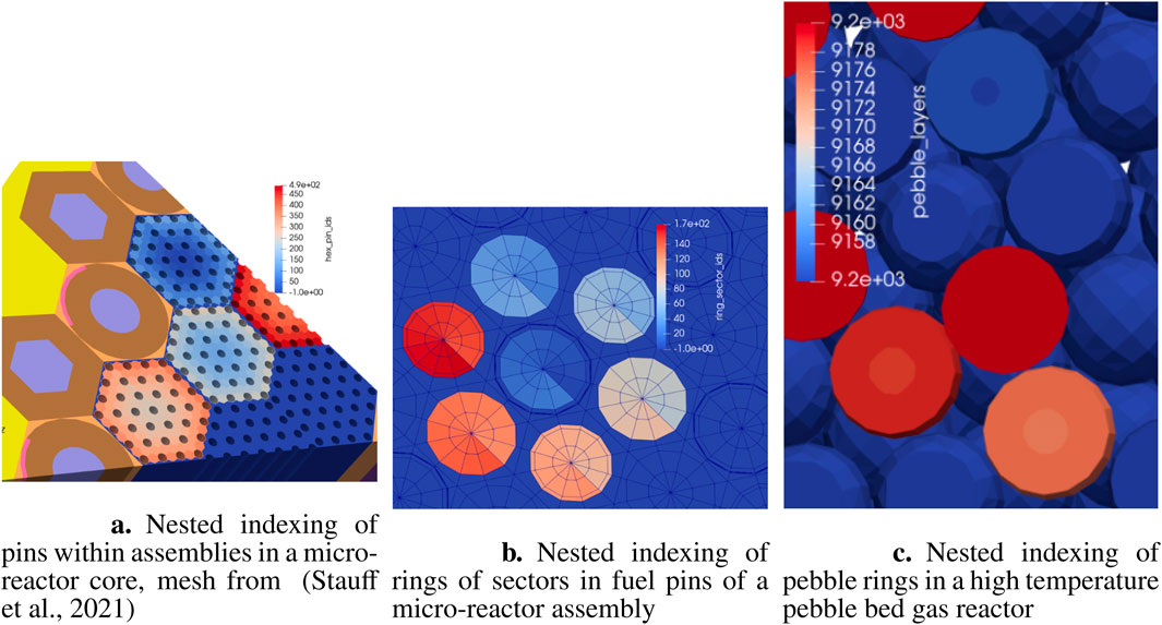
Figure 3. (a) Nested indexing of pins within assemblies in a micro-reactor core, mesh from (Stauff et al., 2021). (b) Nested indexing of rings of sectors in fuel pins of a micro-reactor assembly. (c) Nested indexing of pebble rings in a high temperature pebble bed gas reactor. Mesh divisions used to match transfer regions in advanced reactor cases.

3.6 Coordinate transformations

Different simulations may use different coordinate systems. For example, a neutronics simulation may be performed in Cartesian three-dimensional space whereas a fuel performance calculation may be performed using a two-dimensional axisymmetric coordinate system. Communicating information between these different configurations would be difficult without reconciling the differences in coordinates. One mechanism MOOSE provides for making this communication simpler is the MooseAppCoordTransform class. Each MooseApp instance holds a coordinate transformation object in its MooseMesh object. Users may specify transformation information about their simulation setup on a per-application basis in the input file Mesh block. A coord_type parameter specifies the coordinate system type, e.g., Cartesian, axisymmetric, or radially symmetric. Euler angles are available to describe extrinsic rotations. The convention MOOSE uses for a $\alpha$-$\beta$-$\gamma$ Euler angle rotation is:

1. Rotation about the z-axis by $\alpha$ degrees

2. Rotation about the x-axis by $\beta$ degrees

3. Rotation about the z-axis (again) by $\gamma$ degrees

A length_unit parameter allows the user to specify their mesh length unit. The code in MooseAppCoordTransform which processes this parameter leverages the MOOSE units system. A scaling transform will be constructed to convert a point in the mesh domain with the prescribed mesh length unit to the reference domain with units of meters. The last option which contributes to transformation information held by the MooseAppCoordTransform class is a positions parameter. The value of positions exactly corresponds to the translation vector set in the MooseAppCoordTransform object of the sub-application. The $\alpha$, $\beta$, $\gamma$, and positions parameters essentially describe forward transformations of the mesh domain described by the MOOSE Mesh block to a reference domain. The sequence of transformations applied in the MooseAppCoordTransform class is scaling, rotation, translation, and coordinate collapsing.

The last item in the transformation sequence, coordinate collapsing, is only relevant when information has to be transferred between applications with different coordinate systems. For transferring information from Cartesian to axisymmetric, we must collapse Cartesian coordinates into the axisymmetric space since there is a unique mapping of Cartesian coordinates into axisymmetric coordinates, but not vice versa, e.g., a point in the axisymmetric space has infinitely many corresponding locations in Cartesian space due to rotation about the axis of symmetry. Table 1 summarizes the coordinate collapses that occur when transferring information between two different coordinate systems. The table should be understood as follows, using the first row as an example: for a Cartesian-axisymmetric pairing (e.g., axisymmetric $\to$ Cartesian or Cartesian $\to$ axisymmetric data transfers), both ‘from’ and ‘to’ points will be cast into the axisymmetric coordinate system for the reasoning given above: there is a unique map from Cartesian to axisymmetric, but not vice versa. Similarly for an axisymmetric-radially symmetric pairing (e.g., axisymmetric $\to$ radially symmetric or radially symmetric $\to$ axisymmetric data transfers), both ‘from’ and ‘to’ points will be cast into the radially symmetric coordinate system.

Table 1

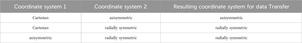
Table 1. Coordinate collapsing.

Note that there are consequences for these coordinate system collapses. When transferring data in the 1 $\to$ two direction, there are (as already stated) infinitely many points in three-dimensional Cartesian space that correspond to a single axisymmetric coordinate. For example, the Cartesian points (1, 0, 0) and (0, 1, 0) map to the same axisymmetric coordinate (1, 0) if the z-axis is the axis of symmetry on the Cartesian mesh. So if we are performing a nearest-node transfer of data from Cartesian to axisymmetric, where the ‘to’ point is (1, 0), then selection of the ‘from’ point is arbitrary if both (1, 0, 0) and (0, 1, 0) points (or any combination of $\sqrt{x^2+y^2}=1$ points) exist. We are considering how best to handle these situations moving forward. One option would be to average the field data from equivalent points. Note that for the axisymmetric coordinate system with general axes, only translation is supported for coordinate transformations, i.e., there is no scaling, rotation, or coordinate collapsing.

3.7 Automated transfer ill-posedness detection

In numerous common transfer setups, there is potential for a non-unique valid source value at a target point. In this event, a single value is still selected, usually the one from the process with the lowest rank. The lowest-rank may not be consistent across different partitionings, so this leads to results that are not consistently reproducible in parallel. These indeterminations occur when, for example:

$•$ Multiple points in the origin mesh(es) are equidistant to the target location for nearest-node type transfers. An example of this case is shown in Figure 4.

$•$ Multiple child apps can compute a valid value for a target location because their meshes overlap, for variable shape/user-object evaluation-type transfers.

Figure 4

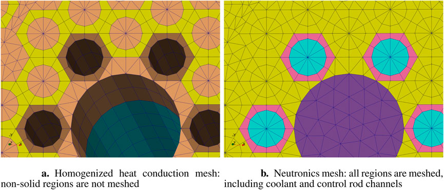
Figure 4. (a) Homogenized heat conduction mesh: non-solid regions are not meshed. (b) Neutronics mesh: all regions are meshed, including coolant and control rod channels. Example of the commonly found indetermination case for the nearest-node transfer. If transferring the graphite matrix temperature from the left heat conduction mesh onto the neutronics mesh on the right (for example, for cross section tabulation purposes), the value at the center of each fuel pin is not uniquely determined with a ‘nearest’ node or element centroid approach.

These issues are detected automatically by the transfers. They can first be discovered when computing the transferred value on the source side. If the child applications presenting the issue are handled by the same process, the multiplicity of valid values is registered when a valid value is requested. If not, then the transfers can also see the indetermination by examining received values from each process for each target point. When multiple values are received for a single target point, the value from the lowest-ranked process is used and, at that point, a potential indetermination is registered.

Finally, at the end of the transfer, global communications are performed to verify that issues discovered when computing the transferred value were actually relevant (e.g., the value selected during that stage was actually the final value for the target point). If another value from another process was selected, then the initially detected indetermination was irrelevant. This global communication is inherently non-scalable and the user is warned if they are deploying it on a case with more than ten processes.

Mesh, block, or boundary restrictions can sometimes be used to alleviate these indeterminations in the origin values. Other times, either re-meshing one of the applications or using the child application positions parameter to create a very small offset can help remove the indetermination. For nearest-node type indeterminations, the recommended fix is to use a local reduction, for example, the average of the nearest-node values using layered averages.

4 Field-to-scalar, scalar-to-field and scalar transfers

In advanced reactor multiphysics core analysis, it is common to have a difference of spatial scale between two physics. Neutronics is typically solved on the global scale for the entire core. On the other hand, fuel performance is typically better solved when considering each disconnected fueled part separately. The fuel performance/thermomechanics of a fuel pin in a light water reactor do not, in most analysis, sufficiently influence the thermomechanics of its neighbor pin to justify a fully-coupled solve including both. Therefore, each pin is best resolved in independent calculations that are pin-scale as opposed to core-scale.

In those cases, while field transfers are still used when both the core-scale and pin-scale meshes are heterogeneous and both resolving the fuel pins, it is often easier to average the local fields and only transfer the average or integrated quantity. It is a simpler approach when the fuel pin meshes do not match. For example, the fuel pin temperature may be averaged over the entire pin before being transferred to the neutronics fuel temperature field. In this case, a scalar quantity is transferred from the distributed fuel performance applications to a field in the global mesh of the neutronics application.

Many coupled cases only require a single scalar number or a few scalars to be passed between applications to couple. This can be, for example, the current insertion height of a control rod that should be shared between the core neutronics calculation and the control rod channel cooling calculation. Domain-overlap coupling of thermal-hydraulics simulations only involve the transfer of a few scalars for the pressure drop, the heat source, and the precursor source for molten salt reactors (Hu et al., 2022).

MOOSE widely supports this transfer mode. Scalars in MOOSE can be Reporters, ScalarVariables or Postprocessors, and all three can be transferred to and from each other with different transfer objects. These transfers are easily distributed as the source values are replicated across all rank using global synchronizations already. This is not a scalable approach but the amount of data is minimal so its impact is not felt in reactor analysis.

5 Advanced reactor multiphysics studies leveraging transfers

5.1 Heat pipe cooled microreactor model

5.1.1 Model description

The HPMR-H₂ is a 2-MW monolithic heat-pipe-cooled microreactor model hosted on the Virtual Test Bed (VTB) repository (Giudicelli et al., 2023). The model, based on the simplified microreactor benchmark problem defined in Ref. (Terlizzi and Labouré, 2023), is composed of 18 hexagonal assemblies arranged into two rings. The tops and bottoms of these 160-cm-high assemblies are surrounded by 20-cm-high axial beryllium reflectors. Each assembly contains 96 fuel pins that are 1 cm in radius, 60 Yttrium Hydride (YH) pins that are 0.975 cm in radius, and 61 1-cm-radius sodium heat pipes drilled into a graphite monolith. The core is surrounded by 12 control drums, with boron carbide employed as the absorbing material. For a simplified mesh, the beryllium radial reflector is hexagonal. The core has a one-twelfth rotational symmetry that allows mitigating the computation burden associated with the simulation. The geometry of the reactor is shown in Figure 5.

Figure 5

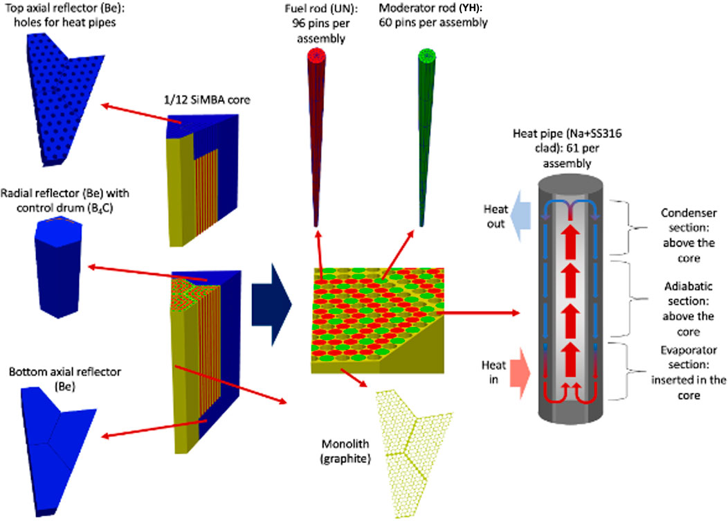
Figure 5. Geometry of the HPMR-H₂ problem.

The HPMR-H₂ model uses Griffin Prince et al. (2024), BISON Williamson et al. (2021), and Sockeye Hansel et al. (2021) to solve the coupled steady-state equations for heterogeneous neutron transport, heat transfer, sodium flow, and hydrogen redistribution. Figure 6 illustrates the computational workflow for the multiphysics simulation. Within the workflow, Griffin is used to solve the multigroup neutron transport equation, BISON is leveraged to simulate both the solid heat transfer and the hydrogen redistribution in the moderator pins, while Sockeye is used to model the sodium flow in the 101 heat pipes. The left box outlines the preliminary steps, including mesh preparation and cross-section tabulations performed using Serpent (v. 2.1.32). Serpent is used due to the existence of a cross section workflow with Griffin at that time. OpenMC and Shift are alternative options with similar workflows. These meshes, along with the cross sections generated, serve as inputs for Griffin, BISON, and Sockeye. For a comprehensive description of the single-physics models, refer to Refs. (NRIC Virtual Test Bed, 2024; Terlizzi and Labouré, 2023).

Figure 6

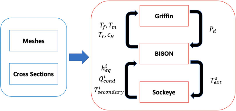
Figure 6. Integrated computational workflow for the HPMR-H₂ problem. Courtesy of (Terlizzi and Labouré, 2023).

5.1.2 Transfers and coupling

As shown in Figure 6, Griffin serves as the parent application for the simulation. It computes the space-dependent multigroup flux distribution by solving the Multigroup Neutron Transport Equation (MNTE). The MNTE is solved with the discontinuous finite element, discrete ordinates (DFEM-SN) approach accelerated with Coarse Mesh Finite Difference (CMFD) acceleration. The power density field, $P_d(\vec{x})$, is then derived from the neutron flux and transferred to BISON via the MultiAppGeneralFieldShapeEvaluationTransfer. This transfer method is chosen because both the Griffin and BISON models are defined at the full-core level, allowing for the evaluation of the source variable’s shape function at the desired transfer location. This transfer was selected because the DFEM-SN solution employs constant monomial variables whereas the BISON model uses first-order Lagrange variables, that are nodal. The use of monomial variables in Griffin was made to decrease the memory requirement in the neutronic simulation.

BISON functions as the daughter application, responsible for computing the temperature distribution in solid materials, $T(\vec{x})$, and the hydrogen-yttrium stoichiometric ratio’s spatial distribution in the YH moderator, $c_H(\vec{x})$. The solid temperature at the heat pipe-monolith interface, denoted as $T_{\mathit{ext}}^s$, is determined from the solid temperature field using layered side averages around each of the 101 heat pipe model instantiations. Each of these instantiations, corresponding to 101 child applications, experiences a different external temperature, which serves as a boundary condition for the fluid solver. The fluid solver then computes the effective heat transfer coefficient $h_{eq}^i$ and secondary temperature $T_{\mathit{secondary}}^i$ for each heat pipe $i$. These computed values are transferred back to BISON to define a convective boundary condition for the solid. Additionally, the heat flux at the heat pipe condenser, denoted as $Q_{\mathit{cond}}^i$, is transferred to BISON to ensure energy conservation between the solid and fluid calculations. Checking the energy balance is crucial due to the different mesh between Sockeye and BISON application. Based on calculation performed through post-processors’ manipulation, we computed that a discrepancy of $0.04\%$ between the heat balance in the solid and the fluid. This discrepancy was deemed sufficiently small to avoid the use of conservative transfers in the simulation. The latter can however be added to enforce conservation of the integral of the energy, as described in Section 3.4.

After iterating between the BISON and Sockeye solutions through a pseudo-transient approach, the steady-state three-dimensional solid temperature distribution is used to determine the fuel, moderator, and reflector temperature distributions, which serve as parameters for the macroscopic cross sections. These partial temperature fields, denoted as $T_f(\vec{x})$, $T_m(\vec{x})$, and $T_r(\vec{x})$, respectively, are then passed back to Griffin through the MultiAppGeneralFieldNearestNodeTransfer together with the hydrogen-yttrium stoichiometric ratio, $c_H(\vec{x})$. Both block restriction and bounding boxes are leveraged to ensure a well-posed transfer process, as detailed in Section 3.7. The Griffin and thermal solution are iterated until the effective multiplication factor converges within a prescribed absolute tolerance, (e.g., 1 per cent mile in the model available on the VTB).

5.1.3 Results

The 3D solid temperature distribution is presented in Figure 7. It is noticeable that the solid temperature is asymmetric with respect to the axial mid-plane due to the heat pipes penetrating only in the top reflector. As a result, fewer neutrons are reflected back into the upper portion of the reactor’s fuel compared to the bottom, leading in turn to an axially asymmetric power generation rate and temperature field. A secondary temperature peak is also evident at the center of the bottom reflector, resulting from the limited heat removal in the central control rod shutdown channel, which is filled with stagnant air. Additionally, the solid temperature distribution at selected axial planes is shown to illustrate the temperature variations at each pin location. A zoomed-in view of the power density, stoichiometric ratio and temperature at the axial mid-plane is provided in Figure 8.

Figure 7

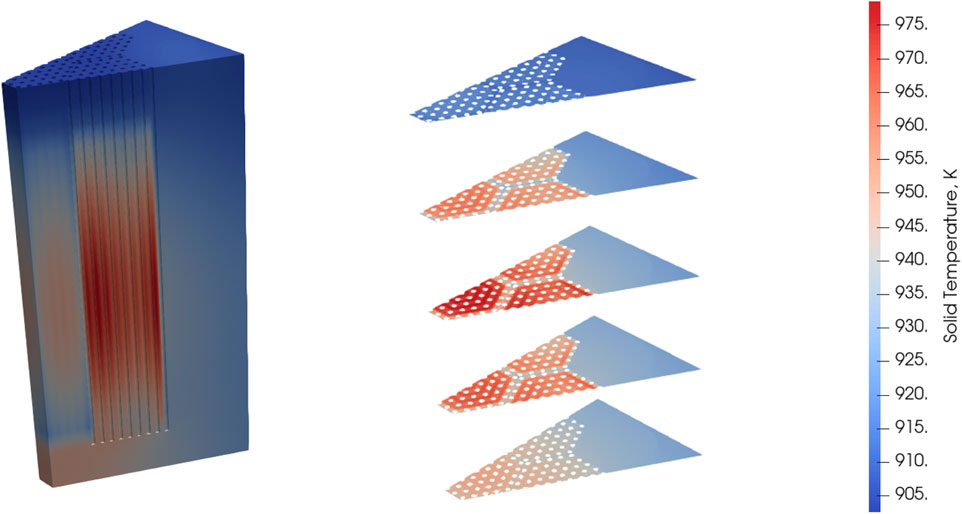
Figure 7. Three dimensional temperature distribution in the solids and 2D spatial distribution for selected axial planes in the HPMR-H₂ problem. Courtesy of (Terlizzi and Labouré, 2023).

Figure 8

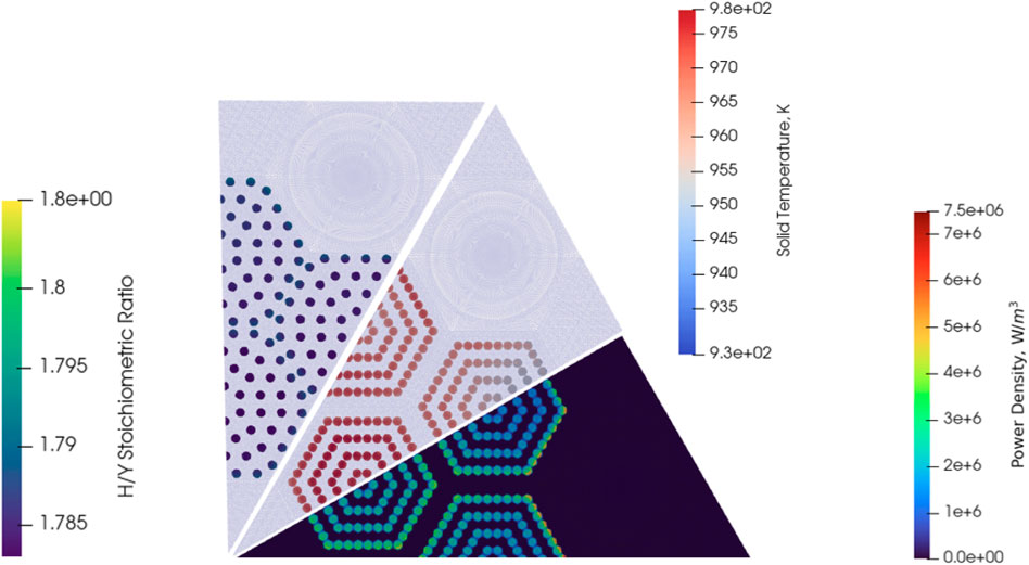
Figure 8. Spatial distributions of quantities of interest at the axial mid-plane in the HPMR-H₂ problem. Courtesy of (Terlizzi and Labouré, 2023).

The temperature of the moderator and the corresponding hydrogen-yttrium stoichiometric ratio are reported as a function of space in Figure 9. It is noticeable that the two quantities are inversely correlated, with the hydrogen redistributing towards colder zones, as expected due to the Soret effect (Terlizzi and Labouré, 2023).

Figure 9

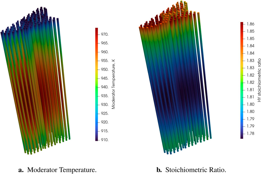
Figure 9. (a) Moderator Temperature Distribution and (b) hydrogen-yttrium stoichiometric ratio in $Y{H}_x$ as a function of space in the HPMR-H₂ problem. Courtesy of (Terlizzi and Labouré, 2023).

5.2 High temperature prismatic gas reactor (HTGR) model

In a prismatic gas-cooled reactor, the fuel is in the form of compacts housed in graphite blocks. The fission heat is transferred to the gas coolant, generally helium, which flows either in an annular flow channel around the fuel rods, as in the High Temperature Test Reactor (HTTR) design, or within dedicated coolant channel holes in the graphite blocks. System-level approaches can be used to model these reactors, but they need an effective thermal conductivity to accurately represent heat conduction in the graphite block. Three-dimensional approaches can more accurately model the heat transfer in the graphite block. These approaches require the evaluation of convective heat transfer in the flow channels for each flow channel location, which can be achieved by modeling the flow channels as child applications created by the heat transfer simulation. This approach is demonstrated on the High Temperature Test Facility (HTTF).

5.2.1 Model description

The HTTF at Oregon State University is a scaled integral effects experiment for investigating transient behaviors in prismatic nuclear HTGRs. The HTTF uses electrical heated rods as the power source and helium as the coolant. A radial cross section of the HTTF core region is shown in Figure 10.

Figure 10

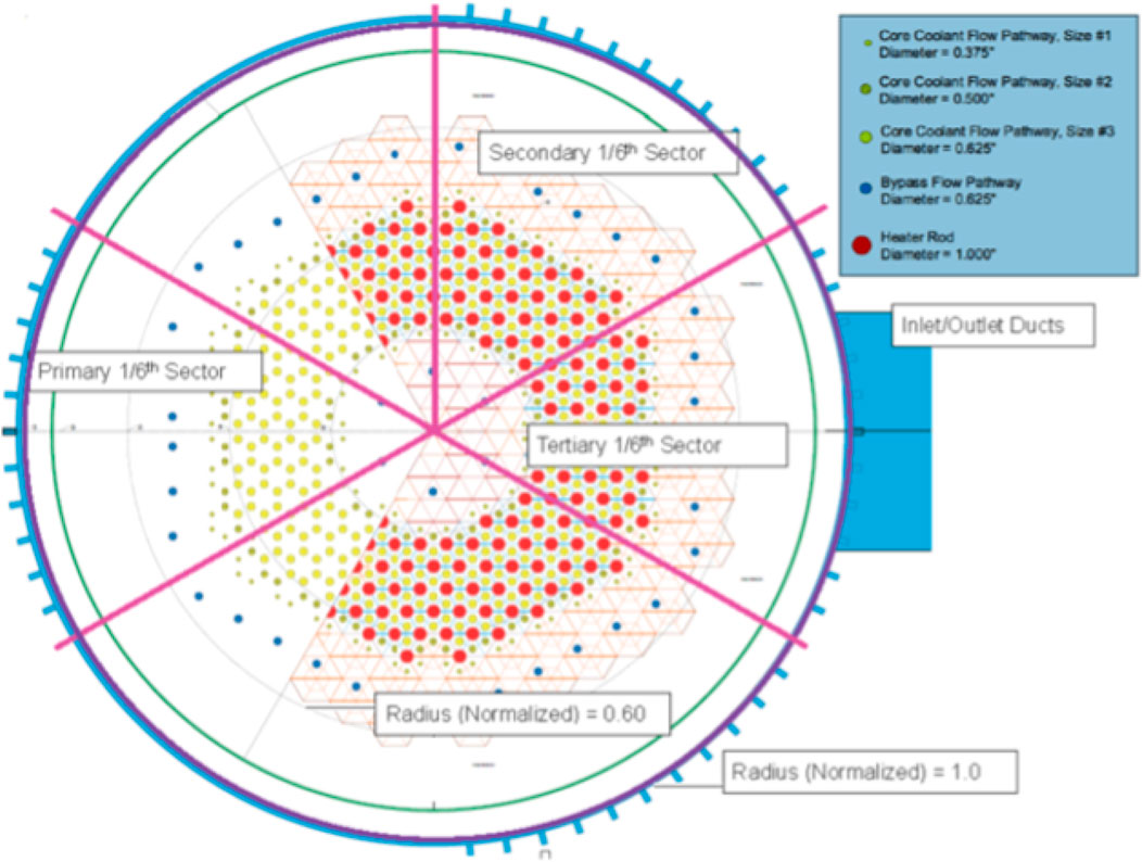
Figure 10. Cross section of the HTTF core block, from Woods (2019).

A 3D mesh of the facility is built and includes the core block with all the coolant flow holes and heater rods holes, the barrel, pressure vessel and the reactor cooling cavity system (RCCS)as shown in Figure 11. A view of the mesh is also shown in Figure 11.

Figure 11

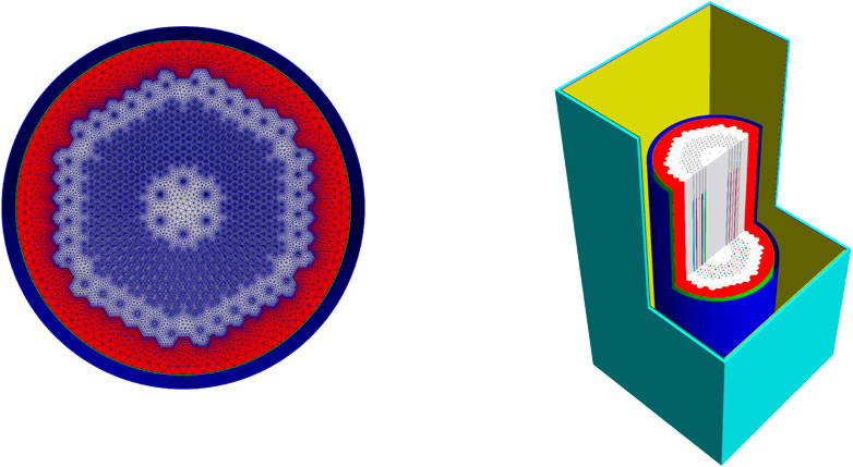
Figure 11. HTTF mesh and model overview.

The heater rods are not explicitly modeled and a heat flux corresponding to the heater power as a function of time is prescribed on the heater holes surface. The heat conduction within the core block is modeled using the MOOSE heat transfer module. A convective boundary condition is applied to the coolant channels walls, on the upcomer walls, and on the RCCS pannel walls. The flow in the coolant channels, upcomer and RCCS channel is modeled using the MOOSE Thermal Hydraulics Model (THM) Hansel et al. (2024). Note that this model is published on the Virtual Test Bed Giudicelli et al. (2023). The heat transfer coefficient in the flow channels is calculated using the modified Dittus Boelter correlation as suggested by McEligot McEligot et al. (1965), and the friction factor is calculated using the Churchill correlation.

5.2.2 Transfers and coupling

The coupling strategy is illustrated on Figure 12. The heat conduction application solving for the heat transfer in the ceramic block is the main application. One SubApp is created for each flow channel within the core block, for the upcomer and for the RCCS water channel.

Figure 12

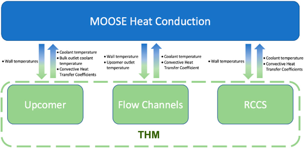
Figure 12. Coupling scheme for the HTTF model.

The temperature on the flow channel walls is averaged by axial layers. Each layers corresponds to an element on the flow channel simulations. This wall temperature is transferred to the channel applications using a MultiAppGeneralFieldUserObjectTransfer object. The heat transfer coefficient is calculated within each channel application and is transferred with the bulk fluid temperature to the main application using a MultiAppGeneralFieldNearestLocationTransfer. The wall temperature, heat transfer coefficient and bulk fluid temperature are used to calculate the convective heat transfer between the core block and the flow channels. A similar approach is used to model the convective heat transfer in the RCCS and upcomer. Note that the upcomer channel has two convective heat fluxes, one on the barrel side and one on the pressure vessel side. Lastly, the upcomer bulk outlet temperature is transferred to the core flow channel application and is used as an inlet boundary condition. A MultiAppPostprocessorTransfer object is used for that purpose.

This model makes use of the nearest-application heuristic to determine which processes should exchange data in the field transfers, see Section 3.5. The default heuristic, based on forming a sphere around each point from the bounding boxes, is rendered inefficient by the elongated bounding boxes of the channel geometries. The nearest-application is a simple concept which suffices here to map regions of the mesh to each channel application.

5.2.3 Results

The transient PG-26 was used as a demonstration. PG26 includes a heatup phase followed by a depressurized conduction cooldown transient. The temperature distribution in the core before the initiation of the depressurization is shown in Figure 13.

Figure 13

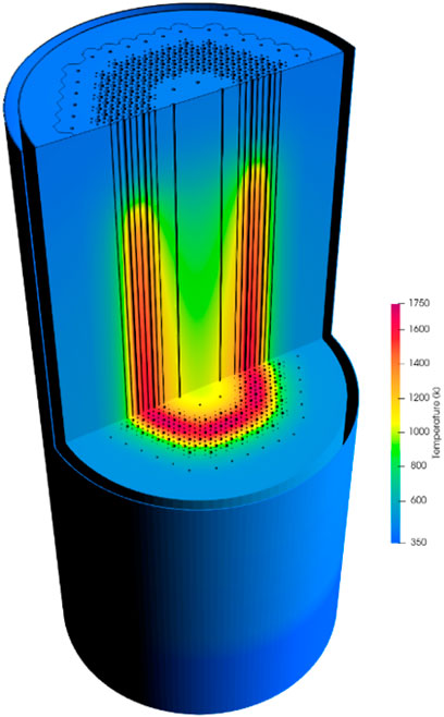
Figure 13. Temperature distribution in the HTTF core block before the depressurization transient.

A comparison of the experimental data with the simulation prediction for the core block solid temperature at the bottom of the core is shown in Figure 14 for each radial ring. A reasonable agreement is reached, especially considering the uncertainties in the measurements.

Figure 14

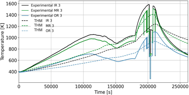
Figure 14. Temperature evolution at the bottom of the HTTF core.

5.3 Molten salt reactors

Molten Salt Reactors are Generation-IV advanced reactor design that is actively pursued by several companies and for which several experiments are planned in the US. Notably, the Molten Chloride Reactor Experiment is scheduled to be build inside the LOTUS test bed of the National Reactor Innovation Center at Idaho National Laboratory. Several molten salt reactor models were developed using the MOOSE-based tools and are available on the VTB Giudicelli et al. (2023). The pool-type core multiphysics model share the same coupling strategy, which was summarized in Subsection 2.2 and in Figure 2. We briefly recall here which features of the transfers are leveraged.

The fluid flow and precursor advection simulations typically use the same mesh, because the velocity field is obtained from solving conservation equations and should not be modified by the transfers or the mesh. Advecting precursors with a non-mass conserving velocity field would create oscillations in the precursors’ distributions. Because they use the same mesh, the simple copy transfer can be used for transferring velocities and Rhie Chow coefficients.

For the other transfers, we have to consider the meshes of the neutronics application compared to the flow applications’. The neutronics application mesh is typically coarser than the fluid application, as the pool-type geometry is homogeneous in the fuel region. The neutronics mesh includes both the salt region and the solid region, with the reflectors and the control rods. In the salt region, it suffices to evaluate the fields in the origin application to recreate them in the target application, as explained in the discussion on shape evaluation transfers in Section 3. The integral of the transferred field is preserved using the rescaling described in Subsection 3.4.

5.4 Fusion device example: a tokamak demonstration model

5.4.1 Model description

This demonstration model consists of a 90-degree sector of a Tokamak. For simplification, the model consists of five domains only: a Tungsten first wall, a Homogenized multiplier layer, a Homogenized breeder layer, a Vacuum vessel, and a divertor. Figure 15 shows the model mesh with different colors for each subdomain. Geometry parameters were taken from (Shimwell et al., 2021). Both the first wall and divertor were modeled as pure Tungsten. The multiplier is a homogenized layer of $65\%$ beryllium, and $35\%$ Helium. The breeder is a homogenized layer of $10\%$ stainless steel alloy, $37\%$ beryllium, $15\%$ ${\text{Li}}_4{\text{SiO}}_4$, and $38\%$ Helium. Finally, the vacuum vessel was modeled as a stainless steel alloy. Natural abundance was assumed for all elements. These compositions were considered for this demonstration model as placeholders where we focused on the modeling workflow and multiphysics solvers transfers.

Figure 15

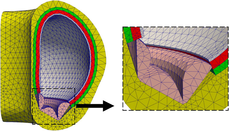
Figure 15. Simplified tokamak model mesh and a zoomed-in view on the divertor; colors correspond to different subdomains.

The model leverages Cardinal (Novak et al., 2022), a wrapping of the Monte Carlo particle transport code OpenMC (Romano et al., 2015) and the spectral element Computational Fluid Dynamics (CFD) code NekRS (Fischer et al., 2022) within the MOOSE framework to allow multiphysics feedback to the particle transport model. A tutorial based on this tokamak model can be found on the Cardinal website (DAGMC Tokamak, 2025).

The tokamak model was first built using capabilities in Paramak (Shimwell et al., 2021), a python package that allows rapid production of 3D CAD models of fusion reactors. Then, the CAD model was imported into Coreform Cubit Blacker et al. (1994) to assign materials, subdomain names, and boundary conditions. Two meshes are then generated for this model: a mesh to solve the heat conduction problem using the MOOSE heat transfer module, and a triangulated surface mesh for transporting particles within OpenMC.

For simplicity, all regions were modeled as purely conducting with no advection considered. This is a significant simplification, and therefore the results obtained should not be taken as representative of a realistic device. The boundary conditions applied to the heat conduction model are also simplified, as the outer boundary temperature is set to a Dirichlet condition of 800 K. All other boundaries are assumed insulated. To approximate some cooling in the breeder and divertor, a uniform volumetric heat sink is applied in these regions.

OpenMC was used for neutron transport by running a series of fixed source calculations on this model. OpenMC and MOOSE are coupled via fixed point iterations through Cardinal. The neutron source was defined as an isotropic ring cylindrical source distributed uniformly inside the cavity of the tokamak with a uniform neutron energy of 14.08 MeV. The cross-section library ENDF/B-VII.1 (Chadwick et al., 2011) was used. The number of particles sampled is $1\times 10^7$ particles per batch. The OpenMC trigger capability (Shen et al., 2015) was used to finish simulations based on tally uncertainties by setting a trigger threshold on the heating tally to finish the simulation at a specified tally relative uncertainty level.

5.4.2 Transfers and coupling scheme

An unstructured mesh-based heat source is calculated in OpenMC using the MOOSE mesh as a tally mesh. The heat source is then transferred to MOOSE via Cardinal to be applied as a volumetric heating term. Heat conduction is solved using the MOOSE heat transfer module and temperatures are calculated. The resulting temperatures are then sent back to OpenMC to account for temperature feedback where one temperature is applied to each OpenMC cell, updating the nuclear interaction cross sections used. Figure 16 illustrates the multiphysics coupling scheme, where temperature feedback is utilized in the OpenMC model to calculate the different neutronic quantities of interest.

Figure 16

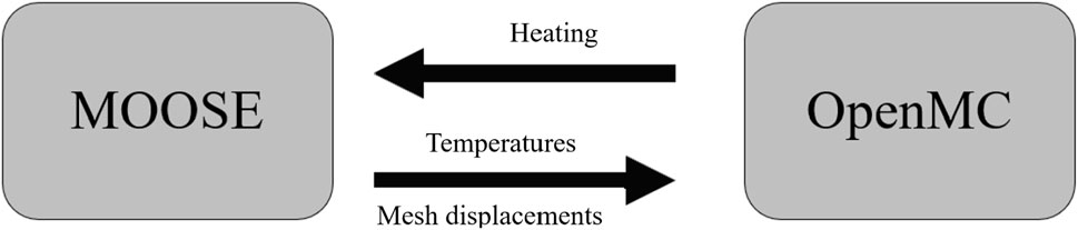
Figure 16. Multiphysics coupling scheme for the tokamak model.

The heat transfer MOOSE module functions as the parent application for the simulation, where it computes temperatures and sends them via the MultiAppCopyTransfer to the Cardinal application which uses an identical mesh for simplicity. The Cardinal daughter application runs at the end of each fixed point iteration to calculate the neutronics quantities of interest (heating, and tritium production) and the heating results are transferred back to the parent application using the MultiAppCopyTransfer.

With recent developments, Cardinal now has the capability to update displacements on OpenMC’s surface mesh geometry from MOOSE’s solid mechanics solver (Eltawila et al., 2025). This allows for utilizing thermomechanical feedback arising from thermal expansion, which will be added as an extension to this tokamak model in future work.

5.4.3 Results

The multiphysics results correspond to a power of 6.1 MW for a 90° sector. Figure 17 shows the simulation results for the neutronics quantities of interest, where we show the solid temperatures computed by MOOSE, on the last fixed point iteration, as well as the tritium production results. Note that these results are not necessarily intended to replicate a realistic tokamak, due to the highly simplified geometry, neutron source definition, and lack of fluid flow cooling. However we can still use this model to estimate the different feedback mechanisms’ importance and demonstrate the workflow.

Figure 17

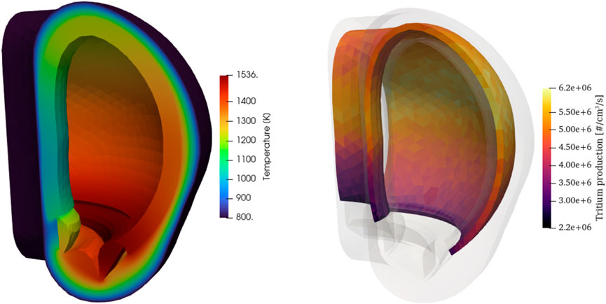
Figure 17. Temperature (left) and tritium production (right) results obtained at 6.1 MW for a 90° sector.

5.5 High fidelity conjugate heat transfer simulations

In the previous section, Cardinal’s use for coupling OpenMC to Multiphysics Object Oriented Simulation Environment (MOOSE) was demonstrated. Cardinal also contains a wrapping of the NekRS spectral element CFD code for a variety of coupling mechanisms, including (i) conjugate heat transfer, (ii) volumetric neutronics feedback, (iii) fluid-structure interaction, (iv) systems-CFD coupling, and (v) forward Uncertainty Quantification (UQ).

5.5.1 Model description

To demonstrate MOOSE’s transfers for conjugate heat transfer applications, we illustrate a simple 7-bin wall-resolved Sodium Fast Reactor (SFR) bundle, where the fluid region is solved with NekRS’s spectral element methods and the solid is solved with MOOSE’s finite element heat transfer module. A tutorial based on this model is available on the Cardinal (2025).

The geometry is a shorter, seven-pin version of the fuel bundles in the Advanced Breeder Reactor (ABR) J. Cahalan and T. Fanning and M. Farmer and C. Grandy and E. Jini and T. Kim and R. Kellogg and L. Krajtl and S. Lomperski and A. Moisseytsev and Y. Momozaki and Y. Park and C. Reed and F. Salev and R. Seidensticker and J. Sienicki and Y. Tang and C. Tzanos and T. Wei and W. Yang and Y. Cahalan et al. (2007). Pin dimensions match those of the full-size reactor, and the bundle power, inlet temperature, and flow rate are scaled so as to obtain laminar flow conditions. While this is not representative of actual turbulent flow SFR conditions, the purpose of the present discussion is to illustrate two different types of heat flux transfers facilitated by MOOSE.

The MOOSE heat transfer module is used to solve for energy conservation in the solid. The outer surface of the duct and the tops and bottoms of the pins and ducts are insulated. Cardinal supports two options for the boundary condition to be applied to the solid-fluid interface, and which necessitate different transfers in MOOSE. These two options are referred to as (i) “flux-flux” coupling, whereby NekRS passes a convective heat flux to MOOSE, $h(T-T_{\infty })$; and (ii) “flux-temperature” coupling, whereby NekRS passes the wall temperature to MOOSE. The gap region between the pellet and the cladding is unmeshed, and a quadrature-based thermal contact model is applied based on the sum of thermal conduction and thermal radiation (across a transparent medium).

NekRS is used to solve the incompressible Navier-Stokes equations. At the outlet, a zero-gage pressure is imposed and an outflow condition is applied for the energy conservation equation. On all solid-fluid interfaces, the velocity is set to the no-slip condition and a heat flux is imposed in the energy conservation equation computed by MOOSE.

The meshes for the solid (MOOSE) and fluid (NekRS) domains are shown in Figures 18, 19. Note that the two applications do not employ a conformal mesh at the fluid-solid interface, which will necessitate nearest node type transfers.

Figure 18

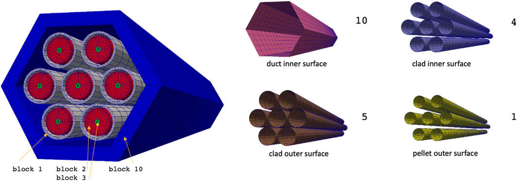
Figure 18. Heat conduction mesh used by the MOOSE heat transfer module. Sideset numbers are listed to the right of each highlighted sideset. Reproduced with permission from Argonne National Laboratory (2024).

Figure 19

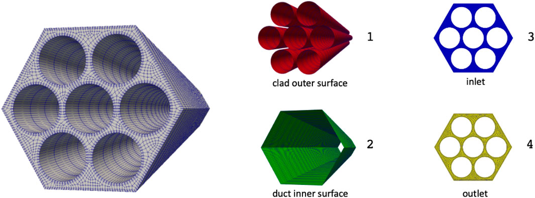
Figure 19. Fluid flow mesh used by NekRS. Sideset numbers are listed to the right of each highlighted sideset. Reproduced with permission from Argonne National Laboratory (2024).

5.5.2 Transfers and coupling scheme

When using conjugate heat transfer coupling, MOOSE passes a conductive heat flux, $-k\nabla T\cdot \widehat{n}$, along the coupled boundary to NekRS. NekRS then either returns the wall temperature as a Dirichlet condition, or a convective heat flux, $h(T-T_{\infty })$. While the wall temperature option, referred to as “flux-temperature” coupling, is fully 3-D, it sometimes requires very frequent data transfers between NekRS and MOOSE to retain stability of the Picard operator splitting. Alternatively, the flux-flux transfer may offer better stability, especially for problems with a large different in thermal conductivity between the fluid and solid, or for high Prandtl number fluids. These two transfer options are summarized in Figure 20.

Figure 20

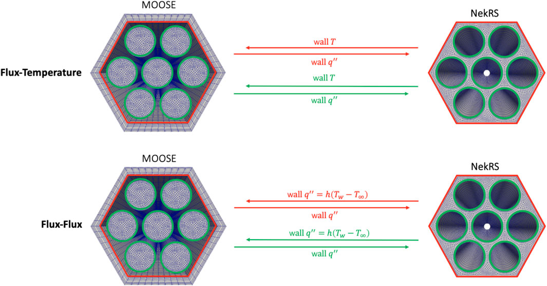
Figure 20. Summary of conjugate heat transfer fields which Cardinal passes between NekRS and MOOSE. Reproduced with permission from Argonne National Laboratory (2024).

The MOOSE transfers used to facilitate these transfers are now described. In order to pass the conductive heat flux from MOOSE to NekRS, a GeneralFieldMultiAppNearestLocationTransfer is employed to pass between nearest nodes on the duct inner surface and clad outer surface sidesets. A nearest node transfer is needed because the use of different meshes in MOOSE and NekRS will not necessarily lead to node overlap. Evaluating the shape function of variables outside of their domain is allowed. In order to account for different side quadrature rules and element refinement, a MultiAppPostprocessorTransfer is also used to pass the side-integrated heat flux (power) from MOOSE to NekRS for an internal normalization step to ensure energy conservation.

The transfer from NekRS to MOOSE then differ depending on the field(s) passed from NekRS to MOOSE. For the flux-temperature coupling option, a MultiAppGeneralFieldNearestLocationTransfer is used to pass NekRS’s wall temperature to MOOSE. Cardinal internally interpolates between NekRS’s Gauss-Lobatto-Legendre (GLL) node points to a MOOSE mesh. For the flux-flux coupling option, UserObjects in Cardinal are used to compute $h$ and $T_{\infty }$ on the NekRS mesh. $T_{\infty }$ represents the bulk-averaged fluid temperature, which is computed directly on the NekRS mesh by subdividing the mesh into sub-volumes. For the present example, each GLL point in the NekRS mesh is mapped to a single subchannel from a typical hexagonal subchannel discretization. For example, Figure 21 shows the indices of each hexagonal subchannel, over which volume averages are used to compute $T_{\infty }$ in sub-volume $i$,

$T_{\infty ,i}=\frac{{\int }_{{\mathrm{\Omega }}_i}TdV}{{\int }_{{\mathrm{\Omega }}_i}dV}(1)$

Figure 21

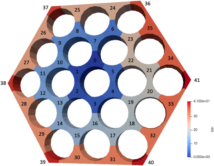
Figure 21. Example of bin indices used for a hexagonal subchannel volume binning, for a 19-pin bundle.

where ${\mathrm{\Omega }}_i$ are the sets of GLL points that would fall into subchannel bin $i$.

To compute the heat transfer coefficient, side-averaged quantities are also required. The index $i$ was used to represent the colored volumes in Figure 21. Using $j$ to indicate the fluid-solid sideset bordering volume $i$, the wall-average temperature and heat flux are computed as

$T_j=\frac{{\int }_{\partial {\mathrm{\Omega }}_j}TdS}{{\int }_{\partial {\mathrm{\Omega }}_j}dS}(2)$

$q_j^{\prime \prime }=\frac{{\int }_{\partial {\mathrm{\Omega }}_j}{q}^{\prime \prime }dS}{{\int }_{\partial {\mathrm{\Omega }}_j}dS}(3)$

where $\partial {\mathrm{\Omega }}_j$ is the sideset pertaining to subchannel $i$. The heat transfer coefficient is then computed as

$h_j=\frac{q_j^{\prime \prime }}{T_j-T_{\infty ,i}}(4)$

UserObjects in Cardinal are used to compute the three quantities on the right-hand side of Equation 4. $h$ is then passed to the MOOSE heat conduction solver as an auxiliary variable using MultiAppGeneralFieldNearestNodeTransfer. $T_{\infty ,i}$ is passed directly as a user object, using MultiAppGeneralFieldUserObjectTransfer which then locally evaluates the value of $h$ at the nodes on the MOOSE heat conduction mesh. $h$ and $T_{\infty ,i}$ are then applied as a Robin-type flux condition using MOOSE’s CoupledConvectiveHeatFluxBC. In other words, using the center pin as an example, the heat conduction model is applied six different values of $h$ and $T_{\infty }$ around the pin circumference to capture the 3-D nature of the heat transfer.

5.5.3 Numerical results and transferred fields

This seven-pin bundle is run with both the flux-temperature and flux-flux coupling options. The fluid and solid temperatures computed with the flux-temperature coupling option are shown in Figure 22. This conjugate heat transfer mode utilizes two MultiAppGeneralFieldNearestNodeTransfers.

Figure 22

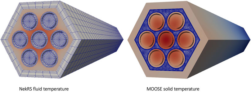
Figure 22. Fluid temperature computed by NekRS (left) and solid temperature computed by MOOSE (right) for the flux-temperature coupling option. Reproduced with permission from Argonne National Laboratory (2024).

Figure 23 shows the solid temperature, when using either the flux-temperature or flux-flux coupling option. For the flux-flux option, the subdomain is divided into 20 axial layers and with a hexagonal subchannel discretization in the $x-y$ plane (18 subchannels). Both options are nearly equivalent, with minor differences because the convective heat flux is not a truly 3-D transfer due to the averaging options required to define $h$.

Figure 23

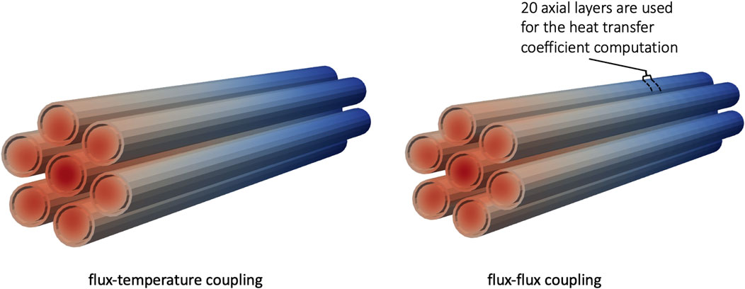
Figure 23. Solid temperature computed by MOOSE when using either the flux-temperature coupling or the flux-flux coupling. Reproduced with permission from Argonne National Laboratory (2024).

6 Conclusion

The coupling of different physics solvers is required for advanced nuclear systems analysis due to the need for specialized solvers to tackle each physics separately. In the MOOSE ecosystem, this is achieved by leveraging the MultiApps and Transfers systems. Over time, those systems have evolved to include numerous refinements such as asynchronous communications, general projection capabilities, sibling transfers, and automated ill-posedness detection. These capabilities support analysis of a wide range of advanced nuclear reactors, several examples of which were shown in Section 5. The scope for planned future developments will focus on concurrency of execution for GPU-CPU applications exchanging data through Transfers, following.

Data availability statement

The original contributions presented in the study are included in the article/supplementary material, further inquiries can be directed to the corresponding author.

Author contributions

GG: Investigation, Methodology, Software, Writing – original draft, Writing – review and editing. FK: Investigation, Software, Writing – original draft. RS: Conceptualization, Investigation, Software, Writing – original draft. LH: Conceptualization, Investigation, Writing – original draft. DG: Conceptualization, Funding acquisition, Software, Writing – original draft. AL: Funding acquisition, Investigation, Project administration, Software, Writing – original draft. ZP: Conceptualization, Software, Writing – original draft. LC: Investigation, Project administration, Writing – original draft. ST: Investigation, Visualization, Writing – original draft. ME: Investigation, Writing – original draft. AN: Investigation, Writing – original draft.

Funding

The author(s) declare that financial support was received for the research and/or publication of this article. This research was partially supported by the Nuclear Energy Advanced Modeling and Simulation program for Modeling and Simulation of Nuclear Reactors under US Department of Energy contract no. DE-AC05-00OR22725.

Acknowledgments

The authors would like to acknowledge the editing contributions of Sarah E. Roberts at Idaho National Laboratory, and the contributions of Quentin Faure to Figure 5. Stefano Terlizzi wants to thank Dr. Vincent Laboure’ for his contribution to the preparation of the heat pipe cooled microreactor model. Thomas Freymann is acknowledged for his contributions to the HTTR model. This research made use of the resources of the High-Performance Computing Center at Idaho National Laboratory.

Conflict of interest

The authors declare that the research was conducted in the absence of any commercial or financial relationships that could be construed as a potential conflict of interest.

Generative AI statement

The author(s) declare that no Generative AI was used in the creation of this manuscript.

Publisher’s note

All claims expressed in this article are solely those of the authors and do not necessarily represent those of their affiliated organizations, or those of the publisher, the editors and the reviewers. Any product that may be evaluated in this article, or claim that may be made by its manufacturer, is not guaranteed or endorsed by the publisher.

Licenses and permissions

This manuscript was authored by Battelle Energy Alliance, LLC under contract no. DE-AC07-05ID14517 with the U.S. Department of Energy. The U.S. Government retains and the publisher, by accepting the article for publication, acknowledges that the United States Government retains a nonexclusive, paid-up, irrevocable, worldwide license to publish or reproduce the published form of this manuscript, or allow others to do so, for United States Government purposes.

References

Argonne National Laboratory (2024). Cardinal website. Available online at: https://cardinal.cels.anl.gov/.

Google Scholar

Blacker, T. D., Bohnhoff, W. J., and Edwards, T. L. (1994). CUBIT mesh generation environment. Volume 1: users manual. Tech. Rep. doi:10.2172/10176386

CrossRef Full Text | Google Scholar

Cahalan, J., Fanning, T., Farmer, M., Grandy, C., Jini, E., Kim, T., et al. (2007). Advanced burner reactor 1000 MWth reference concept. Tech. Rep. doi:10.2172/1349893

CrossRef Full Text | Google Scholar

Cardinal (2025). Conjugate heat transfer for laminar pin bundle flow. Available online at: https://cardinal.cels.anl.gov/tutorials/cht2.html.

Google Scholar

Chadwick, M. B., Herman, M., Obložinskỳ, P., Dunn, M. E., Danon, Y., Kahler, A., et al. (2011). Endf/b-vii. 1 nuclear data for science and technology: cross sections, covariances, fission product yields and decay data. Nucl. data sheets 112, 2887–2996. doi:10.1016/j.nds.2011.11.002

CrossRef Full Text | Google Scholar

DAGMC Tokamak (2025). DAGMC tokamak. Available online at: https://cardinal.cels.anl.gov/tutorials/tokamak.html.

Google Scholar

Eltawila, M., Novak, A., Simon, P., and Giudicelli, G. (2025). Monte Carlo multiphysics on moving meshes: initial verification and case studies. Math. and Comput. Available online at: https://www.ans.org/pubs/proceedings/article-58168/

Google Scholar

Fischer, P., Kerkemeier, S., Min, M., Lan, Y., Phillips, M., Rathnayake, T., et al. (2022). NekRS, a GPU-accelerated spectral element Navier-Stokes solver. Parallel Comput. 114, 102982. doi:10.1016/j.parco.2022.102982

CrossRef Full Text | Google Scholar

Forum, G. I. (2024). Gen-IV advanced nuclear systems. Available online at: https://www.gen-4.org/gif/jcms/c_59461/generation-iv-systems.

Google Scholar

Gaston, D. R. (2019). Parallel, asynchronous ray-tracing for scalable method of characteristics neutron transport on unstructured mesh. (Ph.D. thesis). Massachusetts Institute of Technology. Available online at: https://hdl.handle.net/1721.1/129911

Google Scholar

Gaston, D. R., Forget, B., Smith, K. S., Harbour, L. H., Ridley, G. K., and Giudicelli, G. G. (2021). Method of characteristics for 3d, full-core neutron transport on unstructured mesh. Nucl. Technol. 207, 931–953. doi:10.1080/00295450.2021.1871995

CrossRef Full Text | Google Scholar

Gaston, D. R., Permann, C. J., Peterson, J. W., Slaughter, A. E., Andrš, D., Wang, Y., et al. (2015). Physics-based multiscale coupling for full core nuclear reactor simulation. Ann. Nucl. Energy 84, 45–54. doi:10.1016/j.anucene.2014.09.060

CrossRef Full Text | Google Scholar

Giudicelli, G., Kong, F., Stogner, R., Harbour, L., Gaston, D., Terlizzi, S., et al. (2024a). Data transfers for full core heterogeneous reactor high-fidelity multiphysics studies. Jt. Int. Conf. Supercomput. Nucl. Appl. 302, 05006. doi:10.1051/epjconf/202430205006

CrossRef Full Text | Google Scholar

Giudicelli, G., Lindsay, A., Harbour, L., Icenhour, C., Li, M., Hansel, J. E., et al. (2024b). 3.0 - moose: enabling massively parallel multiphysics simulations. SoftwareX 26, 101690. doi:10.1016/j.softx.2024.101690

CrossRef Full Text | Google Scholar

Giudicelli, G. L., Abou-Jaoude, A., Novak, A. J., Abdelhameed, A., Balestra, P., Charlot, L., et al. (2023). The virtual test bed (vtb) repository: a library of reference reactor models using neams tools. Nucl. Sci. Eng. 197, 2217–2233. doi:10.1080/00295639.2022.2142440

CrossRef Full Text | Google Scholar

Hansel, J., Andrs, D., Charlot, L., and Giudicelli, G. (2024). The MOOSE thermal hydraulics module. J. Open Source Softw. 9, 6146. doi:10.21105/joss.06146

CrossRef Full Text | Google Scholar

Hansel, J. E., Berry, R. A., Andrs, D., Kunick, M. S., and Martineau, R. C. (2021). Sockeye: a one-dimensional, two-phase, compressible flow heat pipe application. Nucl. Technol. 207, 1096–1117. doi:10.1080/00295450.2020.1861879

CrossRef Full Text | Google Scholar

Hu, R., Fang, J., Nunez, D., Tano, M., Giudicelli, G., and Salko, R. (2022). Development of integrated thermal fluids modeling capability for MSRs. Tech. Rep. doi:10.2172/1889653

CrossRef Full Text | Google Scholar

Hu, R., Zou, L., Hu, G., Nunez, D., Mui, T., and Fei, T. (2021). SAM theory manual. Tech. Rep. doi:10.2172/1781819

CrossRef Full Text | Google Scholar

Kirk, B. S., Peterson, J. W., Stogner, R. H., and Carey, G. F. (2006). libMesh: a C++ library for parallel adaptive mesh refinement/coarsening simulations. Eng. Comput. 22, 237–254. doi:10.1007/s00366-006-0049-3

CrossRef Full Text | Google Scholar

Lindsay, A. D., Gaston, D. R., Permann, C. J., Miller, J. M., Andrš, D., Slaughter, A. E., et al. (2022). 2.0 - MOOSE: enabling massively parallel multiphysics simulation. SoftwareX 20, 101202. doi:10.1016/j.softx.2022.101202

CrossRef Full Text | Google Scholar

McEligot, D. M., Magee, P. M., and Leppert, G. (1965). Effect of large temperature gradients on convective heat transfer: the downstream region. J. Heat Transf. 87, 67–73. doi:10.1115/1.3689054

CrossRef Full Text | Google Scholar

Novak, A., Andrs, D., Shriwise, P., Fang, J., Yuan, H., Shaver, D., et al. (2022). Coupled Monte Carlo and thermal-fluid modeling of high temperature gas reactors using cardinal. Ann. Nucl. Energy 177, 109310. doi:10.1016/j.anucene.2022.109310

CrossRef Full Text | Google Scholar

NRIC Virtual Test Bed (2024). Heat pipe microreactor with hydrogen redistribution (hpmr-h2). Available online at: https://mooseframework.inl.gov/virtual_test_bed/microreactors/hpmr_h2/index.html.

Google Scholar

Pawlowski, R. P., Slattery, S., and Wilson, P. (2013). “The data transfer kit: a geometric rendezvous-based tool for multiphysics data transfer,” in Internation conference on mathematics and computation for nuclear science and engineering (Albuquerque, NM, and Livermore, CA (United States): Sandia National Laboratories SNL).

Google Scholar

Prince, Z. M., Hanophy, J. T., Labouré, V. M., Wang, Y., Harbour, L. H., and Choi, N. (2024). Neutron transport methods for multiphysics heterogeneous reactor core simulation in griffin. Ann. Nucl. Energy 200, 110365. doi:10.1016/j.anucene.2024.110365

CrossRef Full Text | Google Scholar

Romano, P., Horelik, N., Herman, B., Nelson, A., Forget, B., and Smith, K. (2015). OpenMC: a state-of-the-art Monte Carlo code for research and development. Ann. Nucl. Energy 82, 90–97. doi:10.1016/j.anucene.2014.07.048

CrossRef Full Text | Google Scholar

Schoder, S., and Roppert, K. (2025). opencfs: open source finite element software for coupled field simulation – part acoustics. arXiv. Available online at: https://arxiv.org/abs/2207.04443

Google Scholar

Schunert, S., Giudicelli, G., Lindsay, A., Balestra, P., Harper, S., Freile, R., et al. (2021). “Deployment of the finite volume method in Pronghorn for gas- and salt-cooled pebble-bed reactors,” in External report INL/EXT-21-63189. Idaho National Laboratory.

Google Scholar

Shen, Q., Boyd, W., Forget, B., and Smith, K. (2015). Tally precision triggers for the OpenMC Monte Carlo code. Trans. Am. Nucl. Soc.

Google Scholar

Shimwell, J., Billingsley, J., Delaporte-Mathurin, R., Morbey, D., Bluteau, M., Shriwise, P., et al. (2021). The paramak: automated parametric geometry construction for fusion reactor designs. F1000Research 10, 27. doi:10.12688/f1000research.28224.1

PubMed Abstract | CrossRef Full Text | Google Scholar

Stauff, N. E., Mo, K., Cao, Y., Thomas, J. W., Miao, Y., Lee, C., et al. (2021). “Preliminary applications of neams codes for multiphysics modeling of a heat pipe microreactor,” in Proceedings of the American nuclear society annual 2021 meeting.

Google Scholar

Terlizzi, S., and Labouré, V. (2023). Asymptotic hydrogen redistribution analysis in yttrium-hydride-moderated heat-pipe-cooled microreactors using direwolf. Ann. Nucl. Energy 186, 109735. doi:10.1016/j.anucene.2023.109735

CrossRef Full Text | Google Scholar

Wang, Y., Schunert, S., Ortensi, J., Gleicher, F. N., Laboure, V. M., Baker, B. A., et al. (2017). “Demonstration of mammoth strongly-coupled multiphysics simulation with the godiva benchmark problem,” in Ans M&C 2017 (Idaho Falls, ID United States: Idaho National Lab. INL).

Google Scholar

Williamson, R. L., Hales, J. D., Novascone, S. R., Pastore, G., Gamble, K. A., Spencer, B. W., et al. (2021). Bison: a flexible code for advanced simulation of the performance of multiple nuclear fuel forms. Nucl. Technol. 207, 954–980. doi:10.1080/00295450.2020.1836940

CrossRef Full Text | Google Scholar

Woods, B. (2019). Instrumentation plan for the OSU high temperature test facility, revision 4. Tech. Rep. Or. State Univ. Available online at: https://www.osti.gov/biblio/1599628

Google Scholar