Q-Finder: An Algorithm for Credible Subgroup Discovery in Clinical Data Analysis — An Application to the International Diabetes Management Practice Study

1. Introduction

Searching for subgroups of items with properties that differentiate them from others is a very general task in data analysis. There are a large number of methods for finding these subgroups that have been developed in different areas of research. Depending on the field of application, the algorithms considered differ in particular on the metrics used to qualify the groups of interest. The field of medicine is one of those where the search for subgroups has had the most applications. Indeed, the considerable heterogeneity in disease manifestation and response to treatment remains a major challenge in medicine. Understanding what drives such differences is critical to adjust treatment strategies, guide drug development, and gain insights into disease progression.

Targeting certain patient populations that would benefit from a particular treatment is becoming an important goal of precision medicine (Loh et al., 2019; Korepanova, 2018). Subgroup analysis (SA) can be used to identify the drivers of this heterogeneity. While confirmatory analyses focus on the assessment of predefined subgroups, exploratory analyses rely on identifying the most promising ones. Exploratory SA is itself divided into two types of approaches, depending on whether it is hypothesis-based or data-driven. In the latter, the analysis is called subgroup discovery (SD). It is widely used to evaluate treatment effect across different groups of patients from various data sources —be it from clinical trials, or real world data. Demonstrating a response to an intervention is a mandatory pathway for regulatory approval of medicines. However, both the limited consideration by standard algorithms of recommended criteria to assess subgroups credibility, or the findings’ lack of statistical power after correcting for multiple testing, hinder the hypothesis generation process and the acceptance of such analyses by healthcare authorities and practitioners (Mayer et al., 2015). In this paper we present Q-Finder, which draws from two families of approaches: the first is Subgroup Identification (SI) and the second is Knowledge Discovery in Databases (KDD).

In the sequel of this section, we first place SD in the context of SA used in clinical studies. We then detail the different SA tasks in clinical research. More specifically, we propose a new classification of SD tasks in a wider context including both SI and KDD which supports presenting a state-of-the-art of SD approaches. We conclude this section by presenting the limits of SD algorithms in the context of clinical research. In Section 2, we describe the Q-Finder algorithm that was designed to address the main limitations of state-of-the-art SD algorithms. In Section 3, we describe the International Diabetes Management Practices Study (IDMPS) database and perform experiments to compare four different algorithms, namely, SIDES (Lipkovich and Dmitrienko, 2014), Virtual Twins (Foster et al., 2011), CN2-SD (Lavrač, 2004), and APRIORI-SD (Kavsek and Lavrac, 2006) on either predictive or prognostic tasks. In Section 4, we discuss the results and the differences between Q-Finder and state-of-the-art algorithms. The last section is dedicated to the conclusion and perspectives.

1.1. Subgroup Analysis in Clinical Research

Randomized Clinical Trials (RCTs) aim to test predefined hypotheses and answer specific questions in the context of clinical drug development. Essentially designed to demonstrate treatment efficacy and safety in a given indication using a limited number of patients with homogeneous characteristics, RCTs are performed in heavily controlled experimental conditions in order to maximize chances to obtain results with sufficient statistical power throughout successive trials. RCTs are the gold standard for evaluating treatment outcomes, although real-life studies can reveal mismatches between efficacy and effectiveness (Saturni et al., 2014). Conversely, Real-World (RW) Data (electronic medical records, claims data, and registries) are mainly generated for administrative purposes, going beyond what is normally collected in clinical trial programs, and represents important sources of information for healthcare decision makers.

In both RCT and RW studies, SA are used to test local effects, for instance, to account for the heterogeneity in the response to treatment. In particular in RCT, SA “has become a fundamental step in the assessment of evidence from confirmatory (Phase III) clinical trials, where conclusions for the overall study population might not hold” (Tanniou et al., 2016). SA include both confirmatory analyses, whose purpose is to confirm predefined hypotheses, and exploratory ones, which aim to generate new knowledge and are exploratory in nature (Lipkovich et al., 2016). When considering a set of patients included in a database, a subgroup of patients is any subset characterized by its extension (all the patients in the subset, e.g., Patient’s ID in {“12345”, “45678”}) and its intension (a description that characterizes the patients in the subset: e.g., “All the adult women”). In SA, a typical type of subgroups of interest are those whose extension corresponds to patients who respond differently to a new treatment (Zhang et al., 2018). A formal definition of subgroups can be found in Lipkovich et al. (2016).

1.2. The Different Subgroup Analysis Tasks in Clinical Research

A key issue in SA in general is to assess and report its results (Rothwell, 2005). In clinical trials, this assessment is critical and depends on the precise purpose of the study. There are different ways to distinguish the purpose of using SA in clinical research. A first distinction relates to the general purpose of the analysis that can be either aimed at studying treatment efficacy or safety, on either a priori defined groups or a posteriori groups. This dichotomous classification is depicted in Figure 1. In the literature, pre‐hoc analysis is most-often called confirmatory analysis, whereas post-hoc analysis is called exploratory analysis (Lipkovich et al., 2016).

FIGURE 1

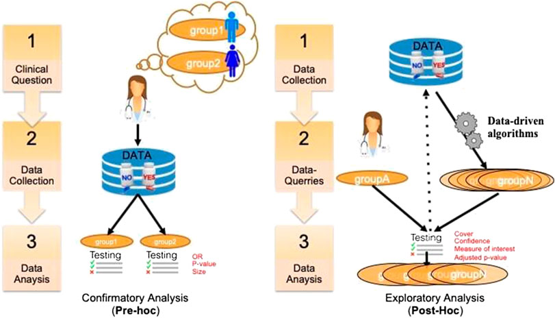
FIGURE 1. A classification of SA tasks distinguishing the confirmatory analyses (left) from the exploratory ones (right).

More recently, Lipkovich et al. (2016) have refined this classification into four different tasks:

(A) Confirmatory subgroup analysis: refers to statistical analysis mainly aimed at testing a medical hypothesis under optimal setting in the absence of confounding factors while strongly controlling the type 1 error rate (using the Family-Wise Error Rate) in Phase III clinical trials with a small number of prespecified subgroups.

(B) Exploratory subgroup evaluation: This refers to statistical analysis aimed at weakly controlling the type 1 error rate (using the False Discovery Rate) of a relatively small number of prespecified subgroups that focuses mostly on “treatment-by-covariate interactions and consistency assessments”.

(C) Post‐hoc subgroup evaluation: refers to non-data-driven statistical post‐hoc assessments of the treatment effect across small sets of subgroups that include responses to regulatory inquiries, analysis of safety issues, post-marketing activities in Phase IV trials, and assessment of heterogeneity in multi-regional studies.

(D) Subgroup discovery: refers to statistical methods aimed at selecting most promising subgroups with enhanced efficacy or desirable safety from a large pool of candidate subgroups. These post-hoc methods employ data mining/machine learning algorithms to help inform the design of future trials.

We propose a decision tree to represent this second classification where the criteria to distinguish Pre-hoc analysis is the strength of type 1 error control (strong or weak respectively), while for Post-hoc analysis, the explicit use of the collected data (hypothesis-driven or data-driven) is considered (see Figure 2).

FIGURE 2

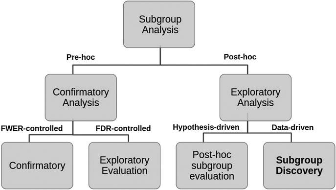
FIGURE 2. Hierarchical tree representing the two layers classification of SA tasks and criteria used.

The sequel of this paper is concerned with exploratory analysis that are based on Data Mining approaches and known as SD. SD has been used in a large number of applications in the medical field and data analysis of randomized clinical trials (Sun et al., 2014).

1.3. Subgroup Discovery: Two Cultures

Two cultures related to subgroup discovery can be distinguished in the literature. The first one is deeply rooted in medical data analysis, biostatistics, and more specifically in the context of drug discovery where both treatments arms and the outcome are key to the analysis. In this domain-specific context (Lipkovich et al., 2016; Lipkovich et al., 2018), that includes either or both candidate covariates and treatment-by-covariate interactions, SD algorithms search either for:

• a global modeling across the entire covariate space (e.g., Virtual Twins (Foster et al., 2011), penalized logistic regression, FindIt (Imai et al., 2013), and Interaction Trees (Su et al., 2009) which extends CART to include treatment-by-covariate interactions);

• a local modeling that focuses on identifying specific regions with desirable characteristic (e.g., SIDES (Lipkovich and Dmitrienko 2014), PRIM (Polonik and Wang, 2010), and TSDT (Battioui et al., 2014)).

The second culture of SD is rooted in the Data Mining and KDD community and applies to any kind of data. The related fields include association rules, set mining, contrast sets, and emerging patterns all relating to the notion of descriptive induction (Fürnkranz et al., 2012).

Although both cultures share common requirements and issues, their vocabulary differs and are practically mutually exclusive in the SD literature. We propose a hierarchical tree representing both cultures and their main associated algorithms (see Figure 3). Since the Q-Finder approach we propose in this paper inherits from both cultures, it is worthwhile giving an account of both of them.

FIGURE 3

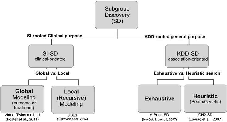
FIGURE 3. Hierarchical tree representing the SD approaches in both biomedical data analysis and data mining cultures. The references under the boxes correspond to representative algorithms of each kind.

In the first culture, where SD is also often referred to as SI (Ballarini et al., 2018; Chen et al., 2017; Dimitrienko and Lipkovitch 2014; Huling and Yu, 2018; Lipkovich et al., 2017; Xu et al., 2015; Zhang et al., 2018), there is a key distinction between prognostic factors (supporting identification of patients with a good or poor outcome, regardless of the treatment assignment) and predictive factors (supporting identification of patients’ response to the treatment) (Adolfsson and Steineck, 2000).

In this culture, SD algorithms¹ can be distinguished depending on whether they search for prognostic and/or predictive factors: the ones that can only look for predictive factors (Quint (Dusseldorp et al., 2016), SIDES, Virtual Twins, and Interaction trees), the ones that only look for prognostic factors (PRIM) and CART (Hapfelmeier et al., 2018)), and the ones that can look for both prognostic and predictive factors (STIMA (Dusseldorp, et al., 2010), and MOB (Zeileis et al., 2008)). The key measures to assess the quality of the SD results in this culture are p-value, type 1 errors, False-Discovery Rate (Lipkovich et al., 2016; Lipkovich et al., 2018).

In the second culture, SD is not associated with a specific sector such as clinical research. On the contrary, SD is defined as “given a population of individuals and a property of those individuals that we are interested in, [the finding of] population subgroups that are statistically the ‘most interesting’, for example, are as large as possible and have the most unusual statistical (distributional) characteristics with respect to the property of interest” (Fürnkranz et al., 2012). More generally, SD “is a type of data mining technique that supports the identification of interesting and comprehensible associations in databases, confirming hypotheses and exploring new ones” (Atzmueller, 2015). These associations are in the form of a set of rules represented as Subgroup $\to$ Target, where Target is the property of interest (e.g., $Hypoglycemia=Yes$) and Subgroup is a conjunction of attribute-selector-value triplets (e.g., $Age>18$ and $Sex=F$). SD belongs to the wider domain of Association Rule mining —this explains why many algorithms bear a name formed from an association rule algorithm and an SD extension —and differs from classical supervised learning as the goal is not to find rules that best predict the target value of unknown observations but rather best support describing groups of observations that when satisfying the condition of a rule also satisfy the target (Fürnkranz et al., 2012).

In this second culture the SD process consists in three main phases: candidate subgroup generation, subgroups evaluation and ranking, and subgroups prunning (e.g., top‐k pruning) (Helal, 2016). The key issues being more related to the algorithmic search for subgroups than their evaluation. This includes the search strategy (be it beam [SD, CN2-SD, and Double-Beam-SD], exhaustive [APRIORI-SD and Merge-SD], or genetic [SD-IGA and SGBA-SD]), stopping criterion (minsup, minconf, maxsteps, etc.) (Valmarska et al., 2017), pruning technique (constraint, minimum support or coverage) and quality measures (confidence, support, usualness [CN2-SD, APRIORI-SD], etc.).

Recent theoretical and empirical analyses have elucidated different types of methods to select algorithms suitable for specific domains of application (Helal, 2016). Applying such algorithms to SA requires considering the outcome as the variable of interest. Nevertheless, the treatment is not explicitly considered as a special variable and dozens of quality measures exist (number of rules, number of variables, support, confidence, precision, interest, novelty, significance, false positive, specificity, unusualness (WRAcc), etc.) (Herrera, 2010).

We will refer to Subgroup Discovery in the context of clinical Subgroup Identification as SI-SD and to Subgroup Discovery in the context of Knowledge Discovery in Database as KDD-SD and compare them with the Q-Finder approach. There is an extensive literature comparing algorithms belonging to each culture independently (e.g., Doove et al., 2013; Zhang et al., 2018; Loh et al., 2019), but to our knowledge, they are not compared when they come from two different cultures.

1.4. Limits of Current Subgroup Discovery Algorithms for Clinical Research

1.4.1. Lack of Statistical Power and Hypothesis Generation

As stated by Burke et al. (2015) “the limitations of subgroup analysis are well established —false positives due to multiple comparisons, false negatives due to inadequate power, and limited ability to inform individual treatment decisions because patients have multiple characteristics that vary simultaneously”. Controlling such errors is a problem: a survey on clinical industry practices and challenges in SD quoted the lack of statistical power to test multiple subgroups as a major challenge (Mayer et al., 2015). As a consequence, SI-SD algorithms often fail to detect any “statistically significant” subgroups.

To control for multiple testing errors SI-SD algorithms often rely on approaches that drastically restrict the number of explored candidate subgroups at the expense of hypotheses generation, usually by using recursive partitioning (Doove et al., 2013). Recursive partitioning approaches could miss emerging synergistic effects, defined as subgroups associated to the outcome, whose individual effects (related to each attribute-selector-value triplet) are independent from the outcome (Hanczar et al., 2010). As such, individual effects combinations would not be selected in tree nodes. Equally, recursive partitioning may also miss optimal combinations of attribute-selector-value triplets, as an optimal selector-value for a given attribute is only defined with relation to previously defined attribute-selector-value triplets² (Hanczar et al., 2010). Therefore, subgroups in output are defined by a combination of variables for which thresholds are not necessarily the optimal ones (with respect to the metrics of interest to be optimized). Furthermore, search space restriction strategies favor the detection of the strongest signals in the dataset, that are often already known and/or redundant from each other.

Finally, pure beam search strategies could miss relevant subgroups as they try to optimize the joint, that is, global, accuracy of all leaves, that is a tree with the most heterogeneous leaves. Consequently, when limiting the complexity (i.e. subgroups length), we can miss interesting local structures in favor of the global picture³ (see Section 6 in Supplementary Materials that shows an example where beam search strategy using a decision tree misses relevant subgroups).

On the contrary, KDD-SD approaches support the exploration of much wider search spaces at the expense of accuracy, as they do not in general control for type 1 errors (be it strong or weak).

1.4.2. Insufficient Credibility and Acceptance of Subgroups

The “Achille’s heel” of SD is the question of credibility of its results. Several meta-analyses have demonstrated that discovered subgroups rarely lead to expected results and have proposed criteria to assess the credibility of findings (Rothwell, 2005). Such credibility metrics are key to support confidence in subgroups and their acceptance by regulatory agencies and publication journals. Several credibility metrics have been provided and recommended (Rothwell 2005; Dijkman et al., 2009; Sun et al., 2010) such as the type of measures of association (relative risk, odds ratio), correction for confounders, correction for multiple testing, as well as treatment-covariate interaction tests.

SI-SD approaches use credibility metrics suited to clinical analyses. However, most of them only provide and consider in their exploration a limited number of credibility metrics (e.g., hypothesis testing p-value), compared to what is recommended in the literature. Moreover, such metrics are rarely consensual. Equally, the subgroups’ generation process (that defines optimal attribute-selector-value triplets combination) mostly relies on the optimization of a limited number of criteria, and is thus not directly driven by all credibility metrics that will be used for the clinical assessment of the subgroups at the end.

On the other hand, KDD-SD can provide a considerable range of credibility metrics as there is no consensus about which quality measures to use (Herrera, 2010), such as WRAcc, Lift, Conviction, Mutual information (Hahsler et al., 2011). However these metrics are seldom used in clinical analyses, hindering their use in the medical field.

Another issue hindering the adoption of SD approaches lies in the comprehensibility of the algorithm itself. This often underestimated issue is an obstacle for convincing clinical teams and regulatory agencies of the relevance and reliability of SD approaches.

2. Q-Finder’s Pipeline to Increase Credible Findings Generation

In this section we present an approach that aims at combining some of the advantages of both SI-SD and KDD-SD cultures, while dealing with limitations observed in current SD algorithms (see Section 1.4). To this end, we introduce Q-Finder, which relies on a four-steps approach (summarized in Figure 4): exhaustive subgroup candidates generation, candidate subgroups assessment on a set of credibility metrics, selection of a limited number of most promising subgroups that are then tested during the final step.

FIGURE 4

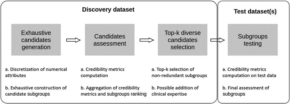
FIGURE 4. Q-Finder works in 4 main stages: an exhaustive generation of candidate subgroups, a ranking of candidate subgroups via an evaluation of their empirical credibility, a selection of the best candidates (taking into account the redundancy between subgroups), and then an assessment of subgroups’ credibility on one or more test datasets.

For further details, an in-depth discussion of Q-Finder is also proposed in Section 14 of supplementary materials. This approach has been applied in several therapeutic areas, with published examples available (Nabholtz, 2012; Eveno, 2014; Amrane et al., 2015; Adam et al., 2016; Dumontet et al., 2016; Gaston-Mathe, 2017; Dumontet et al., 2018; Rollot, 2019; Zhou et al., 2018; Ibald-Mulli, 2019; Zhou et al., 2019; Alves et al., 2020; Mornet, 2020).

2.1. Basic Definitions: Patterns, Predictive, and Prognostic Rules

Numerous formalizations of KDD-SD have been given in the literature. We will briefly introduce some basic definitions of database, individuals, basic patterns, complex patterns, subgroup complexity, and subgroup description related to the ones introduced by Atzmueller (2015). A database is formally defined as $D=\left(I,A\right)$, a set I of N individuals and a set A of K attributes. We will only distinguish nominal and numerical attributes. For nominal attributes, a basic pattern ($a_i=v_{i,j}$) is a Boolean function that is true if the value of attribute $a_i\in A$ is equal to $v_{i,j}$ in the domain of $a_i$ for a given individual of I. For a numerical attribute (be it real or integer) $a_i$, both basic patterns ($a_i\ge v_{i,j}$ ) and ($a_i\le v_{i,j}$) can be defined for each value $v_{i,j}$ in the domain of $a_i$. The associated Boolean function is defined similarly. The set of all basic patterns is denoted by $\text{Σ}$.

A conjunctive language is classically considered to describe subgroups. An association rule $\left(X\to Y\right)$ is composed of a complex pattern (also called itemset) X and a basic pattern Y, where X is called antecedent (or left-hand-side (LHS) or Subgroup) and Y the consequent (or right-hand-side (RHS) or Target). A complex pattern $CP$ is described by a set of basic patterns $CP=\left\{B{P}_1,\dots ,B{P}_k,\dots B{P}_C\right\},B{P}_k\in \text{Σ}$. It is logically interpreted as a conjunction of basic patterns. In other words, a complex pattern $CP$ represents the body of a rule $B{P}_1\wedge \dots \wedge B{P}_C$. In Q-Finder, its length C corresponds to the complexity of the associated rule. The set of observations covered by a complex pattern $CP$ is called the extension of the subgroup, i.e. the individuals for which $CP$ is true $\{x\in I$; CP $\text{is true for x}\}$. In this formalism, the set of all possible association rules is included in the powerset of $\text{Σ}$ although many subsets are not considered because their extension is by construction empty (e.g., $a_i\ge v_{i,j}\wedge a_i\le v_{i,k}\text{ when }{v}_{i,j}>v_{i,k}$). Moreover, this set of all subgroups can be partially ordered in a lattice structure (Ganascia, 1993). We will not rely on such lattice structure because the length of subgroups (i.e. their complexity) is sufficient to partially order the set of generated candidates in subsets.⁴

In SI-SD, many databases include information about treatment distinguishing different individuals grouped in arms. This notion is critical to distinguish two types of rules. The prognostic rules are not related to a treatment effect on a given outcome, unlike the predictive rules.

These two main types of rules can be summarized as follows:

Prognostic rule: “SUBGROUP” $\to$ “TARGET”

Predictive rule: “SUBGROUP” where “TREATMENT” $\to$ “TARGET”

2.2. Preprocessing and Candidate Subgroups Generation in Q-Finder

In Q-Finder, to control the size of the set of basic patterns $\left|\text{Σ}\right|$, all numerical attributes are systematically discretized in bins. A hyperparameter $\#Bins$ sets the maximum number of values $v_{i,j}$ of any numeric attribute $a_i$ (default value: 10). If this number is above $\#Bins$, the attribute $a_i$ is quantized using a discretization method $DiscretizationMethod$ (see algorithm 1 line 8). Different methods exist for quantization, the default one being equal-frequency binning. In the same way, the number of distinct values for a given nominal attribute might be bounded by the hyperparameter $\#Cats$ (default value⁵: $\infty$). If the number of modalities is above this threshold, then a reduction method ($ReductionMethod$) may be used (by default: use the ($\#Cats-1$) most frequent values of $a_i$ and a create a value “other” for all the remaining ones). Let us call Kc the number of nominal attributes and Kb the number of numerical attributes. After this preprocessing step, the number of basic patterns $\left|\text{Σ}\right|$ is bounded and we have the relation: $\left|\text{Σ}\right|\le 2\text{*}Kb\text{*}\#Bins+Kc\text{*}\#Cats$.

Given a set of basic patterns $\text{Σ}$, we call “candidate generation” the search procedure that generates the subgroups (i.e. complex patterns conjunction of basic ones). The number of complex patterns of complexity C is bounded by the number of C-combination of $\text{Σ}$ (i.e. the binomial coefficient $\begin{array}{c}\left|\text{Σ}\right|\\ C\end{array}$). There is extensive literature in KDD-SD on the type of exploration of these complex patterns (Fürnkranz et al., 2012). Experiments have shown that the exhaustive search based methods perform better than other methods which prune the search before evaluation (Helal, 2016). This is particularly true when the problem size is reasonable (i.e. a few thousand individuals) which is mostly the case in SD. The Q-Finder Candidate generation is straightforward; it outputs a subset of all C-combinations of $\text{Σ}$ (with $C\in [1;C_{max}]$) as described below in Algorithm 1.

Algorithm 1: Basic patterns and candidate subgroup generation of complexity $\le$$C_{max}$

1: Input: D, $\#Bins$, $\#Cats$, $C_{max}$ maximum complexity of generated subgroups, $ReductionMethod$, $DiscretizationMethod$

2: $\text{Σ}=$ {} # Set of basic patterns

3: For each nominal attribute $a_i$do

4: If$\#valueof(a_i$) $>\#Cats$then

5:Reduce the number of values of $a_i$ to $\#Cats$ using $ReductionMethod$

6: For each$v_{i,j}$do$\text{Σ}=\text{Σ}\cup \left\{\left(a_i=v_{i,j}\right)\right\}$

7: For each numerical attribute $a_i$

8: If$\#valueof(a_i$) $>$$\#Bins$then

9: Discretize the values of $a_i$ in $\#Bins$ using $DiscretizationMethod$

10: For each$v_{i,j}$do$\text{Σ}=\text{Σ}\cup \left\{\left(a_i\ge v_{i,j}\right),\left(a_i\le v_{i,j}\right)\right\}$

11: $G=$ {} # Set of generated subgroups

12: For each combination s of 1 to $C_{max}$ elements of $\text{Σ}$do

13: If one attribute $a_i$ appears twice or more in s or if the extension of s is empty by construction then skip

14: else$G=G\cup \left\{s\right\}$

15: Output: G the set of generated candidate subgroups of length $\le$$C_{max}$

In practice the Q-Finder algorithm not only supports constructing left-bounded and right-bounded intervals but also supports bounded intervals depending on the number of basic patterns (one or two) associated to a given numerical attribute. If bounded intervals are considered, step 13 of the algorithm becomes “If one attribute $a_i$ appears twice or more in s with the same selector or if the extension of s is empty by construction, then skip”.

2.3. Empirical Credibility of Subgroups

Q-Finder’s candidates generation step may potentially produce a very large number of subgroups. Because of its exhaustive strategy, it produces a number of subgroups which grows exponentially with complexity. Dealing with a massive exploration of database is the challenge of any KDD-SD algorithm be it exhaustive or heuristic, as the number of computed statistical tests may induce a high risk of false positives, that needs to be mitigated.

Q-Finder addresses this challenge by only selecting a subset of candidate subgroups and testing them on independent data, to assess the replicability of the results while controlling the number of tests (and thus the type 1 error). This strategy requires to address two issues:

• a way of evaluating the empirical credibility of subgroups, in order to rank them from most to least promising and

• a top-k selection strategy, in order to select a set of subgroups that seem most credible and will be tested on an independent dataset.

2.3.1. Credibility Metrics

The notion of credibility often appears in the literature on subgroup analysis (Dijkman et al., 2009; Sun et al., 2010; Sun et al., 2012; Burke et al., 2015; Schnell et al., 2016) described according to different criteria. In particular, Oxman and Guyatt (1992) detail seven existing criteria to help clinicians assess the credibility of putative subgroup effects on a continuum from “highly plausible” to “extremely unlikely”. Sun et al. (2010) suggest four additional credibility criteria and re-structure a checklist of items addressing study design, analysis, and context. In the present context, credibility is related to a sequence of a priori ordered statistical metrics that are progressively increasing the confidence (credibility) of a given subgroup. The seven criteria described below are aligned with the clinical domain endpoints (Dijkman et al., 2009; Sun et al., 2010). Using these criteria when selecting the top-ranked subgroups ought to both promote the finding of credible subgroups and facilitate their acceptance by clinicians, agencies, and publication journals.

Drawing from this literature, continuous metrics to measure subgroups’ credibility are used in Q-Finder (more details on literature’s recommendations in relation to Q-Finder metrics in Section 14.4 of supplementary materials). Several credibility criteria are defined, each composed of both a continuous metric and a minimum or maximum threshold (which may be modified by the user):

(1) Coverage criterion: The coverage metric is defined by the ratio between the subgroup’s size and the dataset’s size. This allows to only consider the subgroups that correspond to large enough groups of patients to be clinically relevant. It can be compared to defining a minimum support of the antecedent of a rule in the KDD-SD literature. Default minimum threshold for coverage is $10\text{\%}$.

(2) Effect size criterion: As recommended by both Dijkman et al. (2009) and Sun et al. (2010), Q-Finder’s exploration relies by default on relative risk reductions, which differ according to the probability distribution of the outcome (odds-ratios for discrete or negative binomial distributions, risk-ratios for normal or Poisson distributions, hazard ratios for survival analysis). Those metrics allow to quantify the strength of the association between the antecedent (the subgroup) and consequent (the target) of the rule. Relative risk reductions remain in most situations constant across varying baseline risks, in comparison to absolute risk reductions. In the KDD-SD literature, this continuous metric is usually the confidence (i.e. how often the target is true among the individuals that satisfy the subgroups).The effect size metric may vary depending on whether one is looking for predictive or prognostic factors. When searching for prognostic factors, Q-Finder only considers the effect size measuring the subgroup’s effect (default minimum threshold for effect size is 1.2). When searching for predictive factors, Q-Finder considers simultaneously two effect sizes: the treatment effect within the subgroup and the differential treatment effect, defined as the difference in treatment effect for patients inside the subgroup versus outside the subgroup (see Supplementary Tables S7 and S8 for an example with odds-ratios). When generating predictive factors, one can consider the differential treatment effect on its own, or in combination with the treatment effect within the subgroup. The latter case allows to identify subgroups in which the treatment effect is both positive and stronger than outside the subgroup (default thresholds are 1.0 for the treatment effect within the subgroup and 1.2 for the differential treatment effect).

(3) Effect significance criterion: the association between each subgroup and the target is assessed using a nullity test from a generalized linear model. For the identification of predictive factors, an interaction test is performed to assess between-subgroup treatment effect interactions as recommended by Dijkman et al. (2009). A threshold (typically $5\text{\%}$) is used to define when the p-value related to each effect size metric is considered significant.

(4) Basic patterns contributions criteria: Basic patterns contributions to the subgroup’s global effect are evaluated through two sub-criteria: the absolute contribution of each basic pattern and the contributions ratio between basic patterns.The absolute contributions of a basic pattern is defined by the improvement in effect when this basic pattern is present, compared to the subgroup’s effect when this basic pattern is absent. Each basic pattern contribution should be above a defined threshold (by default 0.2, 0 and 0.2 respectively for the subgroup’s effect, the treatment effect within the subgroup and the differential treatment effect), thus ensuring that each increase in subgroup’s complexity goes along with some gain in effect and therefore in interest.The contributions ratio between basic patterns is the ratio between the maximum absolute contribution and the minimum absolute contribution. A maximum threshold (by default 5 for the subgroup’s effect or the differential treatment effect) is set for this criterion, thus ensuring that basic patterns’ contributions to the subgroup’s effect are not too unbalanced. Indeed, if a basic pattern bears only a small portion of the global subgroup’s effect, then the global effect’s increase is not worth the complexity’s increase due to this pattern’s addition.

(5) Effect size criterion corrected for confounders: the strength of the association is assessed through relative risk reductions (as in criterion 2) while correcting for confounding factors using a generalized linear model. Added covariates are known confounding factors of the outcome, which are susceptible to be unbalanced between patients within and without each subgroup, as well as between treatment arms for predictive factors identification tasks (Dijkman et al., 2009; Sun et al., 2010). As for criterion 2, adjusted relative risks ought to be above a given threshold (same as for criterion 2).

(6) Effect significance criterion corrected for confounders: as for the effect significance criterion (criterion 3) and using the same model as in criterion 5, a threshold (typically $5\text{\%}$) is used to define when the p-value related to each effect size metric corrected for confounders is considered significant.

(7) Effect adjusted significance criterion corrected for confounders: the p-value computed in criterion 6 is adjusted to account for multiple testing, as recommended by Dijkman et al. (2009). This procedure relies on a Bonferroni or a Benjamini-Hochberg correction to control for type 1 errors. As for criterion 6, a threshold is used to determine whether the p-value remains significant after multiple testing correction (typically $5\text{\%}$)

These seven credibility metrics are at the core of Q-Finder. However, they can be further extended by other measures of interest to better fit each research question.

2.3.2. Aggregation Rules and Subgroups Ranking

Aggregation rules are defined to discriminate subgroups according to a set of criteria and therefore to help select the most interesting and/or promising ones for each research question. This is a key concept of Q-Finder, as the goal is to select a set of “top” subgroups before testing them on an independent dataset, whether or not they pass all credibility criteria. In practice, ranking subgroups into aggregation ranks is helpful when no subgroup passes all credibility criteria, and we need to look into lower aggregation ranks to select the most promising subgroups. This approach contrasts with most SI-SD algorithms, where outputs are only subgroups passing all predefined indicators, hindering the generation of hypotheses if these are difficult to achieve.

To this end, a set of credibility criteria is parameterized by the user, depending on the desired properties of the searched subgroups (see Section 2.3.1). Q-Finder computes each metric for each of the candidate subgroups of complexity $C\le$$C_{max}$ and verifies if the associated thresholds are met. A vector of Boolean can thus be associated to each subgroup depending on which thresholds are met, and are used to order the candidate subgroups, according to prespecified aggregation rules.

By default, Q-Finder prioritizes subgroups that meet the following credibility criteria: subgroups with a minimal value of coverage (coverage criterion), defined by basic patterns that sufficiently contribute to the subgroup’s effect (basic patterns contribution criteria), with a minimal level of effect size adjusted for confounding factors⁶ (effect size criterion corrected for confounders) and adjusted p-values for multiple testing below a given level of risk (effect adjusted significance criterion corrected for confounders). Please note that the above-mentioned effect could either be the subgroup’s effect size (for prognostic factors) or the treatment effect within the subgroup and/or the differential treatment effect (for predictive factors). Aggregation rules are the following (from least to most stringent):

• Rank 1: subgroups that satisfy the coverage criterion;

• Rank 2: subgroups of rank 1 that also satisfy the effect size criterion;

• Rank 3: subgroups of rank 2 that also satisfy the basic patterns contribution criteria;

• Rank 4: subgroups of rank 3 that also satisfy the effect significance criterion;

• Rank 5: subgroups of rank 3 or 4 that also satisfy the effect criterion corrected for confounders;

• Rank 6: subgroups of rank 5 that also satisfy the effect significance criterion corrected for confounders;

• Rank 7: subgroups of rank 6 that also satisfy the effect adjusted significance criterion corrected for confounders.

These aggregation rules can be visualized through a decision tree (see Supplementary Figure S8). One can notice that subgroups with an odds-ratio adjusted for confounders but not significant (rank 5) are ranked before subgroups with significant odds-ratios (not adjusted for confounders, rank 4) for hypotheses generation. This ranking is consistent with favoring adjusted odds-ratios with a lack of statistical power to potential biased estimates. As well as the possibility of adjusting the list of parameters, the order of priority between parameters can also be changed to take into account different priorities.

In addition, a continuous criterion is chosen to sort subgroups of the same aggregation rank. Classically, the criterion called Effect significance criterion corrected for confounders is preferred. This is consistent with recommendations by Sun et al. (2010) that state that the smaller the p-value, the more credible the subgroup becomes. In case of a tie, additional criteria can be used to determine the final ranking, such as the effect size criterion corrected for confounders, to favor subgroups with stronger effect sizes. This ranking procedure is summarized in algorithm 2.

Algorithm 2

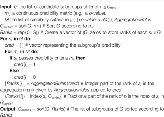
Algorithm 2: Ranking candidate subgroups

2.4. Q-Finder Subgroups Diversity and Top-k Selection

2.4.1. Subgroups Diversity

Q-Finder performs a subgroups top-k selection to be tested on an independent dataset. One of the known issues in KDD-SD of top-k mining algorithms is that they are prone to output redundant subgroups as each subgroup is considered individually. Several authors including Leeuwen and Knobbe (2012) have argued to search for subgroups that offer a high diversity: diverse subgroup set discovery. Therefore, the goal is to take into account the fact that many subgroups might be redundant either extensionally (their basic patterns are very similar) or intensionally (the objects covered by the subgroup are similar). A general approach to address this issue is to define a redundancy measure. It can for example consider the number of common attributes between two subgroups, or the percentage of common examples covered by two different subgroups. The last requires more computation but results in a better diversification of subgroups as it considers possible correlations between variables.

Q-Finder proposes a definition of intensional redundancy between basic patterns, where two basic patterns (attribute-selector-value triplets, respectively $a_1-s_1-v_1$ and $a_2-s_2-v_2$) are considered redundant if:

• $a_1=a_2$

• AND:

• For nominal attributes: $v_1=v_2$

• For numerical attributes:

• $s_1=s_2$

• OR considering $s_1$ as ”$\le$” and $s_2$ as ”$\ge$”, $v_1\ge v_2$

Based on the basic patterns redundancy definition, two subgroups are called redundant if $C_{min}$ basic patterns are redundant between them; $C_{min}$ being the minimum complexity of the two subgroups.

2.4.2. Selection of Top-k Subgroups to Be Tested

Different strategies exist to identify an optimal top-k selection of non-redundant subgroups (Xiong et al., 2006), based on subgroups’ intensions, extensions, or both. In addition to those existing strategies, Q-Finder proposes its own approach based on subgroups’ intensions (see Algorithm 3) to determine an optimal set of k non-redundant subgroups $S_k$ from the ranked set of generated subgroups $G_{ranked}$ (output from Algorithm 2).

The best candidate subgroup is iteratively selected using 2 continuous metrics : $m_c$ from Algorithm 2 and another continuous metric. This top-k algorithm was originally designed using a p-value metric⁷ for $m_c$ and an effect size⁸ for the second metric⁹. For the sake of clarity, we will describe this algorithm using those 2 metrics:

• Subgroups should be selected from less complex to most complex (favoring less complex subgroups);

• When two subgroups of equal complexity are redundant, only the one associated with the best p-value should be retained.

• When two subgroups of different complexities are redundant

• The most complex subgroup of the two is discarded iff its chosen effect size metric is lower than the less complex one;

• The less complex subgroup of the two is discarded iff both its chosen p-value and effect size metric are respectively higher and lower than the more complex one.¹⁰

This top-k selection process based on these principles is detailed in Algorithm 3.

Algorithm 3

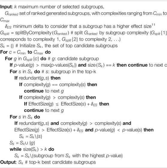
Algorithm 3 Q-Finder’s iterative top-k selection based on subgroups’ intensions

2.5. Possible Addition of Clinical Expertise

Clinical input can be used to overrule algorithm’s preference during top-k selection, by removing candidate subgroups from $G_{ranked}$ (the set of candidate subgroups cf. Algorithm 3) or force the addition of a subgroup into $S_k$ (the set of best candidates cf. Algorithm 3). The result of this step is a set of most promising non-redundant subgroups, that has a maximum size of k. More generally, clinical experts can directly select top-k relevant subgroups among the most credible ones. This stage, that is sometimes referred to as Interactive Machine Learning (Holzinger, 2016), is aligned with the American Statistical Association recommendations that encourage researchers for seeking experts judgement in any statistical analysis, including for evaluating the importance and the strength of empirical evidence (Wasserstein et al., 2019). By integrating experts into Q-Finder’s process for subgroups selection, one allows the consideration of non-measurable properties, such as the novelty, interest or applicability of the proposed subgroups¹².

2.6. Subgroups’ Generalization Credibility

In Q-Finder the final step consists in computing the credibility metrics of the top-k subgroups on the testing set, in order to assess their generalization credibility, that is subgroups consistency across databases (Dijkman et al., 2009; Sun et al., 2010). However, contrary to the candidate subgroups generation phase previously performed, the number of tested subgroups in this phase is well-controlled (as recommended in Dijkman et al., 2009 and Sun et al., 2010), as it is limited by the parameter k. This allows a better control of the type 1 error that was more difficult to achieve until then. For that purpose, Q-Finder performs a correction for multiple testing during computation of the significance metrics, to account for the number of subgroups tested on independent data (default: Benjamini-Hochberg procedure). Top-k subgroups satisfying the credibility criteria on the test dataset are considered highly credible.

3. Experiments and Results

This section is dedicated to compare Q-Finder with representative algorithms for predictive or prognostic SD. First, the IDMPS database on which experiments were run is described. Then, the research questions are stated and both a prognostic and a predictive task are described. Lastly, four different methods and their results are given and compared with Q-Finder.

3.1. Introduction of the International Diabetes Management Practice Study Database

The International Diabetes Management Practice Study (IDMPS) database is an ongoing international, observational registry conducted in waves across multiple international centers in developing countries since 2005. Each wave consists of a yearly 2-weeks fact-finding survey, which aims to document in a standardized manner: practice environments, care processes, habits, lifestyle and disease control of patients with diabetes under real world conditions. It has recently led to new findings related to the suboptimal glycemic control in individuals with type 2 diabetes in developing countries and the need to improve organization of care (Aschner et al., 2020). Observational registries for patients suffering such conditions are pivotal in understanding disease management. In 2017, an estimated 425 million people were afflicted by diabetes worldwide, with Type 2 Diabetes Mellitus (T2DM) accounting for approximately $90\text{\%}$ of cases. By 2030, diabetics should represent $7.7\text{\%}$ of the adult population, or 439 million people; and 629 million people by 2045 (Shaw et al., 2010; Chen et al., 2012; Ogurtsova, 2017). The two most recent waves to date of IDMPS (wave 6 [2013–2014] and wave 7 [2016–2017]) were selected for the following experiments, including data from 24 countries from Africa, Middle East, India, Pakistan, Russia and Ukraine. Only data from patients having T2DM and taking either a Basal insulin, a combination of Basal and Prandial insulin or a Premixed insulin were included.

3.2. Research Questions

3.2.1. Prognostic Factors Identification

One of the main goals of the IDMPS initiative is to evaluate patient’s disease management. To do so, a key outcome in diabetes is the blood level of glycated hemoglobin (HbA1c). High HbA1c is a risk factor for micro- and macrovascular complications of diabetes (Wijngaarden et al., 2017). Patients with T2DM who reduce their HbA1c level of 1% are 19% less likely to suffer cataracts, 16% less likely to suffer heart failure and 43% less likely to suffer amputation or death due to peripheral vascular disease (Dennett et al., 2008; Alomar et al., 2019).

Given the importance of HbA1c control for diabetics patients, we deemed interesting to focus our prognostic factors detection on patients meeting the recommended HbA1c threshold. This recommended threshold varies depending on several factors, such as age or history of vascular complications. For most T2DM patients, this threshold is set at 7%, which is how we define glycemic control for TD2M patients. Our research question can then be formulated as follows: “What are the prognostic factors of glycemic control in TD2M patients?”. We consider the following variables as confounding factors: Patient’s age (Ma et al., 2016), Gender (Ma et al., 2016), BMI (Candler et al., 2018), Level of education (Tshiananga et al., 2012) and Time since diabetes diagnosis (Juarez et al., 2012). Considering the geographical heterogeneity in IDMPS, we added the continent where the data was collected.

This experiment included 1857 patients from IDMPS wave 6 and 2330 patients from IDMPS wave 7, with 63 variables considered as candidate prognostic factors. In wave 6, $17.7\text{\%}$ of patients were under the $7\text{\%}$ HbA1c threshold, versus $18.8\text{\%}$ in wave 7.

3.2.2. Predictive Factors Identification

Another key outcome in diabetes management is the occurrence of hypoglycemia events, which is one of the main complications linked to diabetes. Hypoglycemia symptoms include dizziness, sweating, shakiness; but can also lead to unconsciousness or death in severe cases. Previous studies have shown the impact of insulin treatments on the incidence of hypoglycemia, including comparing premixed insulin analogues to basal insulin analogues (with or without prandial insulin). In some cases, hypoglycemia rates were found to be slightly higher in patients population treated with premixed insulin analogues (Petrovski et al., 2018).

We focused our predictive factors detection on hypoglycemia risk in the past 3 months under premixed insulin versus basal insulin (alone or in combination with prandial insulin).

Our research question can then be formulated as follows: ”What are the subgroups in which the treatment effect (premixed insulin versus basal insulin with or without prandial insulin) on the risk of hypoglycemia in the past 3 months is both positive and higher than outside the subgroups?” Illustrative example: ”The risk ratio in experiencing hypoglycemia under premixed insulin versus basal insulin (with or without prandial insulin) is greater on male patients than on female patients”.

This experiment included 2006 patients from IDMPS wave 6 and 2505 patients from IDMPS wave 7, with 62 variables considered as candidate predictive factors. In wave 6, 32.4% of patients were taking Premixed insulin with a hypoglycemia rate of 32.2%, versus 25.6% for basal insulin regimen. In wave 7, 39.0% of patients were taking Premixed insulin with a hypoglycemia rate of 33.1%, versus 28.3% for basal insulin regimen.

3.3. Analytical Strategies

An objective of this paper is to compare the Q-Finder algorithm to state-of-the-art approaches for clinical SD in both SI-SD and KDD-SD. There are a vast number of approaches in both domains, we chose two state-of-the-art methods from KDD-SD to address the prognostic factors research, and two methods from SI-SD to address the predictive factors research. Among SI-SD methods, we chose SIDES (Subgroup Identification Differential Effect Search method) and Virtual Twins. The first one is arguably the most well known local recursive methods while Virtual Twins is a recognized method, representative of global modelling approaches. In the domain of KDD-SD methods, we chose APRIORI-SD and CN2-SD which are well-known representative of respectively exhaustive and heuristic approaches to SD.

While these four methods do cover the spectrum of SD and identification methods, both SIDES and Virtual Twins are well adapted to predictive tasks, APRIORI-SD and CN2-SD can only address prognostic tasks. Since Q-Finder can address both tasks, it is compared with the two methods that are adapted to each of the two tasks described in Section 3.2. For all the analyses, IDMPS wave 6 were used as the discovery dataset and IDMPS wave 7 as the test dataset. To allow comparison of results, only the top-10 subgroups of each algorithm are considered without any human intervention during the selection. Finally, default parameters of each algorithm were selected, except shared parameters which we kept as similar as possible.

3.3.1. Exploring Prognostic Subgroups

For each of the three approaches to identify prognostic subgroups (CN2-SD, APRIORI-SD, and Q-Finder) we detail the version and main parameters.

CN2-SD¹³: A beam search algorithm adapted from association rule learning CN2 to SD. It introduces a weighted covering method, where examples covered by a subgroup are not removed from the training set but their weights are decreased. This allows examples to appear in several subgroups and cover groups with more diversity. The version used is the one found in Orange 3.23.1. The default parameters are: $WRAcc$ as the optimisation metric, $beam\_width=20$ (the bigger the beam, the more combinations are tested), $max\_rule\_length=3$ (parameter representing the maximum complexity of a subgroup¹⁴) and $min\_covered\_examples=10\text{\%}$ (minimum coverage of a subgroup¹⁵).

APRIORI-SD¹⁶: An exhaustive search algorithm adapted from association rule learning APRIORI to SD. Compared to APRIORI it only considers subgroups that contain the target variable in the right-hand side. Like CN2-SD, it also uses the weighted covering method. The Python package pysubgroup version 0.6.1 (Lemmerich and Becker, 2018) is used, with the following parameters: $WRAcc$ as the optimisation metric, $maxdepth=3$¹⁴ and $result\_set\_size\_coverage=10\text{\%}$¹⁵.

Q-Finder prognostic mode: The version used is 5.4 with $C_{max}=3$, #$Bins$ = 10 and #$Cats$ = $\infty$ (see Section 2.2). Only left-bounded and right-bounded intervals are considered. The thresholds for credibility criteria are the default values presented in Section 2.3.1 : minimum coverage = 10%, minimum basic pattern absolute contribution = 0.2, maximum basic pattern contribution ratio = 5, minimum effect size = 1.2 (with or without correction for confounders), and maximum effectś significance threshold = 0.05 (with or without correction for confounders). Multiple testing correction is addressed using Bonferroni correction in the discovery dataset and Benjamini-Hochberg procedure in the test dataset. For the ranking steps, aggregation rules are the ones presented in Section 2.3.2, $m_c$ being the p-value for subgroup’s effect when corrected for confounders. The default top-k selection is performed with the odds-ratio corrected for confounders as the second metric and ${\delta }_{ES}=0.2$ (see Section 2.4.2).

3.3.2. Exploring Predictive Subgroups

For each of the three approaches to identify predictive subgroups (Virtual Twins, SIDES and Q-Finder) we detail the version and main parameters.

Virtual Twins¹⁷: Following the vignette’s recommendation from the R package aVirtualTwins version 1.0.1, missing values were a priori imputed on the discovery dataset using $rfImpute\left(\right)$ from the randomForest package version 4.6.14. For this step and each of the following, the $seed$ was set to 42. After the imputation, Virtual Twin’s first step consisted in using randomForest() from the randomForest package (version 4.6.14) with $ntree=500$ and $threshold=0.5$ (threshold above which the treatment effect is considered significant for a patient). The second step consisted in performing a classification tree with $maxdepth=3$ (maximum depth of the classification tree¹⁴). Only the leaves for which the predicted outcome was the target were considered as outputted subgroups.

SIDES¹⁸: The version considered is 1.14 from the SIDES R package. The parameters considered are: $M=5$ (maximum number of best promising subgroups selected at each step of the algorithm), $alpha=0.05$ (overall type 1 error rate, which is compared with p-values corrected for multiple testing using a resampling-based method to protect the overall type 1 error rate), $S=200$ (minimum subgroup size desired, set at 10% of the discovery dataset¹⁵), $L=3$ (maximum depth of the tree¹⁴), $D=0$ (minimum difference between the treatment and the control arm), $gamma=1$ (relative improvement parameter), $num\_crit=1$ (splitting criterion used: maximizing the differential effect between the two child subgroups), $H=1$ (i.e. no random split of the discovery dataset), $ord.bin=10$ (number of classes continuous covariates are discretized into¹⁹). As SIDES is a non-deterministic algorithm, the $seed$ was set to 42.

Q-Finder predictive mode: The version used is 5.4 with $C_{max}=3$, #$Bins$ = 10 and #$Cats$ = $\infty$ (see Section 2.2). Only left-bounded and right-bounded intervals are considered. The thresholds²⁰ for credibility criteria are the default values presented in Section 2.3.1 : minimum coverage = 10%, minimum basic pattern absolute contribution = (0, 0.2), maximum basic pattern contribution ratio = ($\infty$, 5), minimum effect size = (1, 1.2) (with or without correction for confounders), and maximum effectś significance threshold = (0.05, 0.05) (with or without correction for confounders). Multiple testing correction is addressed using Bonferroni correction in the discovery dataset and Benjamini-Hochberg procedure in the test dataset. For the ranking steps, aggregation rules are the ones presented in Section 2.3.2, $m_c$ being the p-value for differential treatment effect when corrected for confounders. Nevertheless, they are additional intermediate ranks to account for criteria with 2 thresholds (one for treatment effect within the subgroup, the other for differential treatment effect):

• Rank i: threshold met for treatment effect within the subgroup only;

• Rank i+1: threshold met for differential treatment effect only;

• Rank i+2: threshold met for both treatment effect within the subgroup and differential treatment effect.

The default top-k selection is performed with the odds-ratio for differential treatment effect corrected for confounders as the second metric and ${\delta }_{ES}=0.2$ (see Section 2.4.2).

3.4. Results

3.4.1. Prognostic Factors Identification

Q-Finder results on the prognostic task: Q-Finder generated 203 subgroups satisfying all the credibility criteria. Among the top-10 subgroups selected while accounting for diversity, 2 are of complexity 1, none are of complexity 2 and 8 are of complexity 3. The results are presented below in Table 1 along with the main metrics of interest computed on both the discovery and the test datasets (see Supplementary Table S14 for the additional metrics computed and outputted from Q-Finder). The two first-ranked subgroups S1 and S2 are both of complexity 1 and state that patients whose last postprandial glucose (PPG) level was below 172.0 mg/dl (resp. whose last fasting blood glucose (FBG) level was below 129.6 mg/dl) do have a better glycemic control than the others. Both subgroups are very close to the glycemic control targets established by the American Diabetes Association (resp. 180 mg/dl for PPG and 130 mg/dl for FBG, (American Diabetes Association, 2017)). The coverage (or support) of the first subgroup S1 is $30\text{\%}$ of the discovery dataset, its adjusted odds-ratio is 4.8 ([3.5; 6.5]) and its p-value is $1.81E-23$ on the discovery dataset. All selected subgroups were successfully reapplied on the test dataset, with odds-ratios corrected for confounders above 1.81 and p-values below 0.05 when adjusted for multiple testing by Benjamini-Hochberg procedure. It is worth noticing that all the subgroups were significant using the more conservative Bonferroni correction in the discovery dataset.

TABLE 1

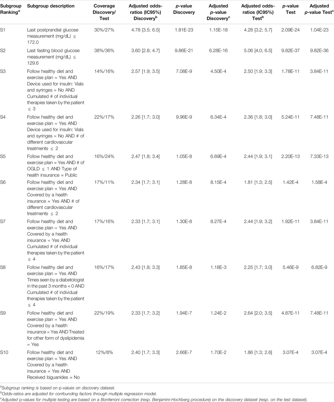
TABLE 1. Q-Finder results on the detection of prognostic factors describing patients with better glycemic control.

Results for CN2-SD and APRIORI-SD:

Results for both CN2-SD and APRIORI-SD are given below. For CN2-SD, no subgroups were outputted using the default parameters, described in 3.3.1. An analysis of the sensitivity is presented in the discussion of the results (see Section 4.2). For APRIORI-SD, 186 subgroups were outputted. Among the top-10 subgroups based on the WRAcc measure, 1 is of complexity 1, 2 are of complexity 2 and 7 are of complexity 3. The complexity 1 subgroup (S4 in Table 2) is defined by a last postprandial glucose measurement below 144 mg/dl (WRAcc on discovery dataset: 0.0329). All complexity 2 and 3 subgroups, except S10, are also defined by this basic pattern, combined with other patterns such as $ReceivesGLP-1analogues=No$ or $Self-monitoringtestingperformedatbedtime=No$. The results are presented below in Table 2 with the WRAcc measure, both on the discovery and the test datasets.

TABLE 2

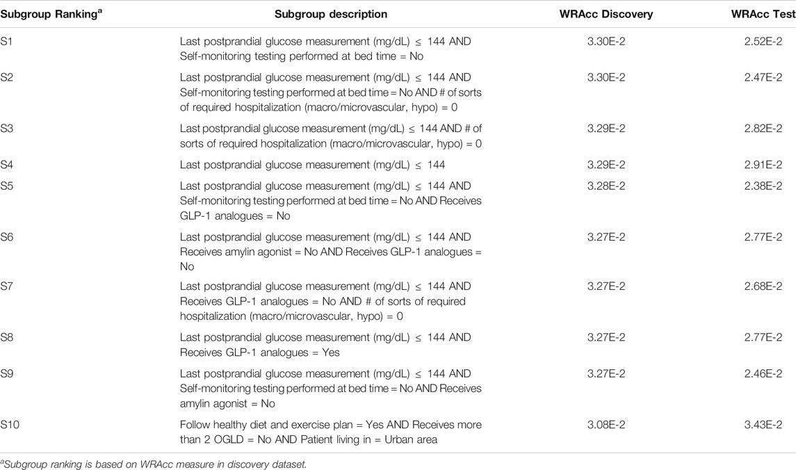
TABLE 2. APRIORI-SD results on the detection of prognostic factors describing patients with better glycemic control.

3.4.2. Predictive Factors Identification

Q-Finder results on the predictive task: Q-Finder generated 2775 subgroups in the discovery dataset that pass all the criteria of credibility on the predictive task. Among the top-10 subgroups selected while accounting for diversity, all are of complexity 3 except one. The results are presented below in Table 3 with main criteria of interest computed on both the discovery and the test datasets (see Supplementary Tables S15 and S16 for the additional metrics computed and outputted from Q-Finder).

TABLE 3

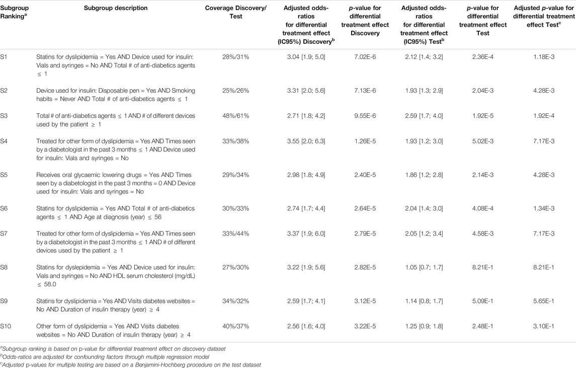
TABLE 3. Q-Finder results on the detection of predictive factors describing patients with a higher risk than the others in experiencing hypoglycemia under Premixed insulin than under Basal insulin (with or without Prandial insulin).

Subgroup S2 states that patients who use a disposable pen, don’t smoke and are not heavily treated for diabetes, have a higher risk than the others in experiencing hypoglycemia under Premixed insulin than under Basal insulin (coverage = 25%, adjusted odds-ratio for differential treatment effect = 3.31 [2.0 ; 5.6], p-value = 7.13E-6).

The seven first selected subgroups were successfully reapplied on the test dataset, with adjusted odds-ratios related to differential treatment effect above 1.86. Indeed, these subgroups have a p-value below 0.05 adjusted for multiple testing using Benjamini-Hochberg procedure, despite the fact that no subgroups were ”statistically significant” after Bonferroni correction in the discovery dataset. It is worth noticing that all subgroups have adjusted odds-ratios above 1.0 in the test dataset.

Results for SIDES and Virtual Twins on the predictive task: Results for both SIDES and Virtual Twins are given below. For SIDES, no subgroups were outputted using the default parameters, described in Section 3.3.2. An analysis of the sensitivity is presented in the discussion of the results Section 4.2. For Virtual Twins, only three subgroups were obtained, 1 of complexity 2 and 2 of complexity 3. The results are presented below in Table 4 with the metrics that are outputted from the algorithm, both on the discovery and the test datasets. All subgroups are defined by a same attribute, the ”number of different lipid-lowering agents for dyslipidemia”.

TABLE 4

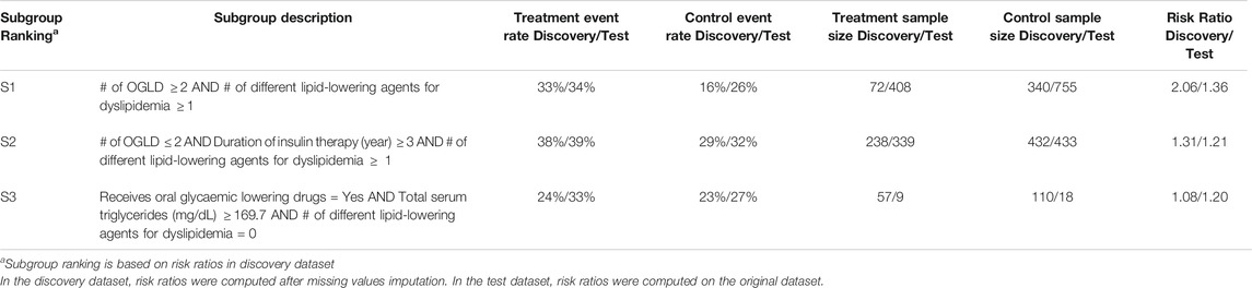
TABLE 4. Virtual Twins results on the detection of predictive factors describing patients with a higher risk than the others in experiencing hypoglycemia under Premixed insulin than under Basal insulin (with or without Prandial insulin).

4. Discussion

4.1. Discussion of the Results

For clarity we discuss the results in relation to Q-Finder for both the search of prognostic factors and predictive factors.

4.1.1. Q-Finder Generates the Top-k Hypotheses

Q-Finder has proposed 10 prognostic factors and 10 predictive factors. This is more than the set of subgroups generated by Virtual Twins and conversely to SIDES and CN2-SD that did not generate any subgroups with their default parameters This illustrates that with default parameters Q-Finder systematically gives results whose credibility are assessed.

As for SIDES, the lack of results may well be explained by the strategy it uses to generate hypotheses. Indeed, SIDES filtering strategy, in which subgroups have to pass all predefined criteria in the learning phase (including the p-value corrected for multiple testing, a very conservative step), strongly limits hypotheses generation. The absence of results is therefore not uncommon with SIDES. On the contrary, the top-k selection strategy of Q-Finder favors the generation of hypotheses since the k best-ranked subgroups of the discovery dataset will be considered as hypotheses to be tested on independent data. This both allows to assess Q-Finder’s results robustness, while preserving the statistical power (as only k tests are performed in the test dataset). Therefore, conversely to SIDES, the correction for multiple testing that is performed in the discovery dataset (that both gives more credibility to the results from the learning phase and increases the subgroups discrimination in the ranking phase) does not hinder the most promising subgroups to be tested and possibly validated on an independent dataset. Q-Finder is thus aligned with the notion of ”statistical thoughtfulness”²¹ recently promoted by the American Statistical Association (Wasserstein et al., 2019).

For CN2-SD, the lack of results may be due to the beam search, which does not cover the entirety of the search space and may thus miss relevant subgroups. Indeed, in a pure beam search strategy, the search for subgroups of higher complexity is based on the ones of lower complexity. This can therefore lead to missing subgroups, notably to favor the overall accuracy at the expense of local structures²². Equally, beam search strategies could miss subgroups with optimal thresholds, as stated in Section 1.4. Indeed, the ability to perform an exhaustive search allows Q-Finder to find the optimal selector-values for each combination of attributes that meet as much as possible the set of credibility criteria (as defined in Section 2.3. This point is illustrated in Table 1 with subgroups S3 and S8, where the attribute-selector pair “Cumulated number of individual therapies taken by the patient$\le$” is associated with the value 3 or 4 depending on the context of the other basic patterns). Finally, non-exhaustive searches can also miss the detection of emerging synergistic effects, that have probably also been ruled out by SIDES, since the null (or very small) individual effects of each basic pattern would not be selected in a node of a tree. Nevertheless, one of the major advantages of beam search is related to its memory consumption. Since the algorithm stores only a limited number of basic patterns at each level of the search tree, the size of the memory in the worst case is $O\left(Bm\right)$, where B is the beam width, and m is the complexity of the subgroup. It is also faster as only the B most promising subgroups of complexity m are considered to explore the subgroups of complexity $m+1$.

4.1.2. Credibility of the Generated Subgroups: Q-Finder Favors the Generation of Credible Subgroups

By searching for subgroups that meet the recommended and standard credibility criteria for clinical research, Q-Finder makes it possible to directly target promising and credible subgroups for their final clinical evaluation. More precisely, subgroups are assessed on their coverage and effect sizes adjusted for confounding factors, on their adjusted p-values for multiple testing, and the contribution of each basic pattern to the overall relationship with the outcome. Like most SI-SD algorithms for the search of predictive factors (e.g.: MOB, Interaction Trees, STIMA, …), SIDES and Virtual Twins only cover a limited number of these credibility criteria (see Supplementary Table S10). SIDES and Virtual Twins for example do not drive the subgroups generation on risk ratios corrected for known biases (i.e. the “confounding factors”, which are already known as being associated with the outcome). Therefore, the results generated by SIDES and Virtual Twins are possibly biased and have thus a higher risk of being ruled out afterwards during their clinical assessment. Similarly, SIDES and Virtual Twins may have ruled out subgroups that could have held after correcting for confounding factors.

This is even more obvious for CN2-SD and APRIORI-SD, whose detection of prognostic factors are based on a main criterion: the WRAcc. This criterion represents a trade-off between coverage and effect. Although widely used in the KDD-SD community, it is neither conform with the standards in clinical research, nor corrected for confounding factors (see Supplementary Table S9).

For all these algorithms, the identified subgroups may thus be ruled out during their posterior evaluation by the metrics of interest. Moreover, although the adjusted effect sizes of all APRIORI-SD subgroups appear high in both discovery and test datasets they are redundant. In fact, several subgroups sharing the same basic patterns are associated with the very same extension (as suggested by the identical results on credibility measures in the discovery dataset), which masks the fact that they are the same subgroups (e.g., S1 and S2 as well S3 and S4 in Table 5). The fact that an increase in complexity is not always accompanied by an increase in effect is due to the fact that APRIORI-SD does not include any parameters evaluating the contribution of basic patterns (such as the Q-Finder basic patterns contribution criteria), which leads to unnecessarily more complex subgroups. Finally, one can see that adjusted effect sizes of Virtual Twins subgroups are mostly smaller than those of the Q-Finder subgroups, and that none of the three subgroups generated by Virtual Twins have p-values below 0.05 once confusion biases have been corrected in the test dataset (Table 6). Based on the credibility criteria used in clinical research, Virtual Twins has therefore generated less convincing results than Q-Finder.

TABLE 5

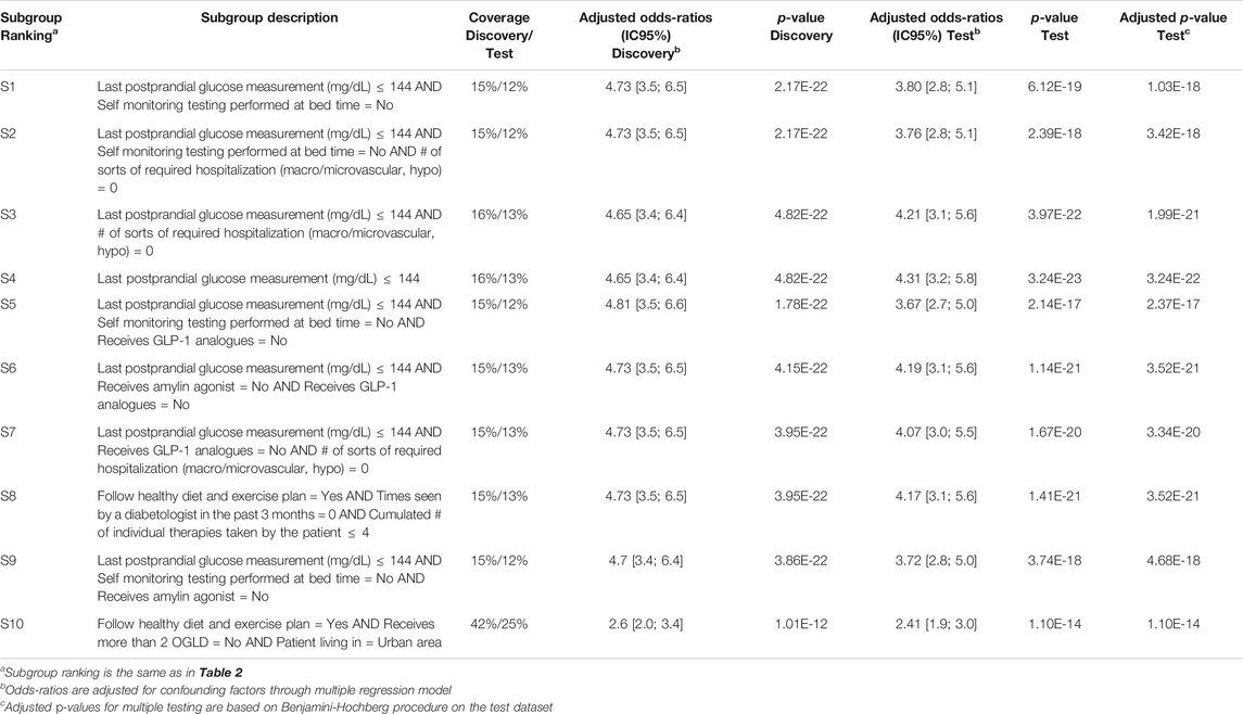
TABLE 5. Credibility metrics from literature (used in Q-Finder) computed on APRIORI-SD results.

TABLE 6

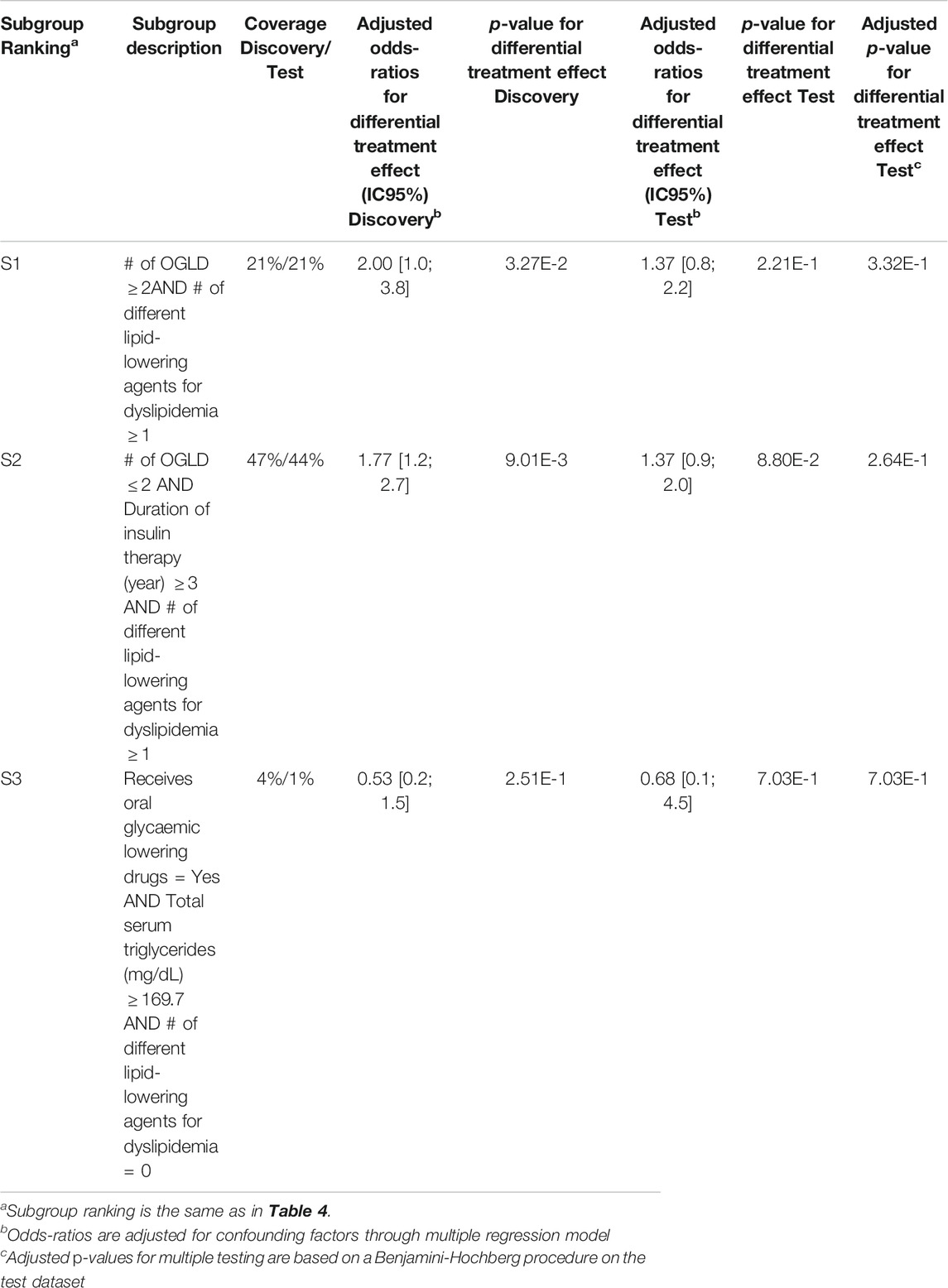
TABLE 6. Credibility metrics from literature (used in Q-Finder) computed on Virtual Twins results.

Moreover, whether Virtual Twins, APRIORI-SD or CN2-SD, the robustness of the results is not meant to be evaluated on independent data. Similarly, they do not seek to control and assess the risk of false positives, regardless of their presence in the results. This seriously undermines the credibility of the results.

4.1.3. Better Supporting Subgroups

Q-Finder supports the set of subgroups with standard and recommended criteria of credibility in clinical research. Therefore, all metrics used in Q-Finder for generating hypotheses are given as outputs for transparency. As strongly recommended by the American Statistical Association (Wasserstein et al., 2019):

• p-values are reported in continuous. This should allow experts to better interpret them, and avoid basing any decision on a p-value threshold that would misrepresent what ”worthy” and ”unworthy” results are.²³

• p-values can be “interpreted in lights of its context of sample size and meaningful effect size”. This set of metrics is key for scientific inference of results.

Q-Finder also provides confidence intervals of effect sizes, to help experts to assess results.

This is to be contrasted with most packages, including the ones used in this paper to compare Q-Finder. Indeed, Virtual Twins package only gives information about size and risk ratios (not adjusted for confounding factors). The SIDES package would only output continuous p-values below an arbitrary threshold. As for CN2-SD and APRIORI-SD, we are far from the standards for the publication of prognostic factors (see Supplementary Tables S11 and S12 for comparison of output metrics from standard packages). As a result, using only a subset of the recommended credibility metrics to both generate and evaluate the subgroups leads to less well-supported results and a higher risk of a posteriori discarding them.

4.1.4. Diversity: Q-Finder Favors the Generation of Various Subgroups and Limits Redundancy

By combining an exhaustive search and an innovative selection algorithm, Q-Finder has made it possible to promote the generation of subgroups whose descriptions differ, for both prognostic and predictive factors (see Table 7 and Table 8 that compare the subgroups diversity level between algorithms). Overall, diversity on subgroups description is less present in subgroups from Virtual Twins which only generated 3 subgroups all defined by the ”number of different lipid-lowering agents for dyslipidemia” attribute. For APRIORI-SD, which generated a large number of subgroups, 9 out of 10 subgroups are defined by the same basic pattern (”last postprandial glucose measurement$\le$144 mg/dl”). In addition, note that those of the APRIORI-SD subgroups which are excessively complex (as indicated in Section 4.1.2) would have been avoided by Q-Finder’s top-k selection algorithm, for which an increase in complexity requires an increase in effect.

TABLE 7

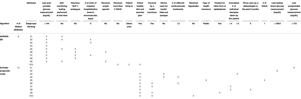
TABLE 7. Prognostic subgroup diversity visualization per attribute and selector-value pairs.

TABLE 8

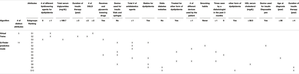
TABLE 8. Predictive subgroups diversity visualization per attribute and selector-value pairs.

However, we observe that 8 out of the top-10 Q-Finder prognostic subgroups share a basic pattern (i.e. ”Follow healthy diet and exercise plan = Yes”). The results could be further improved by using other types of diversity algorithms based on the subgroups’ extensions (see Supplementary Section 14.6 regarding redundancy). The known draw-back of searching for extensional redundancy is related to its higher computational cost. One could also note that several basic patterns although not syntactically redundant do share a similar clinical meaning (e.g., “Statins for dyslipidemia = Yes” and “Treated for other form of dyslipidemia = Yes” are both about taking a dyslipidemia treatment). This is explained by the fact that several attributes in the dataset contain related information. Stricter pre-selection of attributes, based on both correlation analysis and clinical expertise before performing the analysis, is a classic approach to reduce this type of redundancy.

4.2. Limits of the Experiments

4.2.1. Algorithms Used for Benchmarking

We only considered two algorithms for the detection of prognostic factors (CN2-SD and APRIORI-SD) and two algorithms for the detection of predictive factors (Virtual Twins and SIDES) for the experiments. These algorithms have been chosen because they are representative of SI-SD and KDD-SD algorithms. Although it would be interesting to compare with other algorithms (such as MOB, STIMA, Interaction Trees, …) to strengthen the key messages delivered in this paper, a simple review of the literature on these algorithms allows to generalize some of these messages, whether on the ability to target suited hypotheses or on the ability to support them with recommended credibility metrics.

Equally, we only used default thresholds of the algorithms, except when it was relevant in view of the comparison between algorithms (e.g., we used the same coverage value of 10%). One can argue that other thresholds could have been tested to improve the algorithms’ outputs. However, the goal is not here to prove the deficiencies of other algorithms through these experiments, but to generate elements of discussion that shows Q-Finder specificity and the source of its power (e.g., regarding the optimized metrics, the outputs metrics, etc). Nevertheless, a limited analysis of parameters sensitivity was performed for both SIDES and CN2-SD which did not generate any subgroups with the default set of parameters. For SIDES, we explored an increase of the threshold of significance to 0.2 and a decreased maximum number of best promising subgroups selected at each step to 1. Only the first case produced a single candidate subgroup (see below, p-value = 0.066 corrected for multiple testing using a resampling-based method to address the overall type 1 error rate). This subgroup is “close” to some of the top 10 predictive subgroups in Q-Finder, which supports the results obtained with Q-Finder:

Receives oral glycaemic lowering drugs = Yes AND

Treated for other form of dyslipidemia = Yes AND

Visits diabetes websites = No

For CN2-SD, we explored a slight increase of the beam parameter to 50 and a decreased coverage parameter to 5%. No results were obtained in the first case, and the second case did generate 2 subgroups of complexity 3 that share two attributes (see Supplementary Table S13 for the results). More generally, sensitivity analyses are recommended in any SD tasks, by marginally modifying algorithms parameters or the outcome definition (e.g.: $HbA1c<7.5\text{\%}$ instead of $7\text{\%}$).

4.2.2. Limits of the International Diabetes Management Practice Study Databases: Surveys

As the IDMPS databases are derived from surveys spread over time, they each reflect an image at a given time. As a result, treatment initiation may have occurred before data recording. In this situation, the data studied are not necessarily the baseline of the study, which gives the results a purely descriptive character. Indeed, a variable by which a subgroup is defined should not be affected by treatment response (Dijkman et al., 2009). The most common use case of SD is rather the retrospective study of prospective data (e.g., RCT) or real world data, in which temporal information is collected, in order to only consider the information before treatment’s intake (i.e. the ”baseline” period).

4.3. Generalization to Other Pathologies or Research Questions

Q-Finder was applied in the field of diabetes to many other research questions, such as the detection of patient profiles that benefit the most of SGLT2i compared to DDP4i in terms of renal function preservation, using Electronic Health Record data (Zhou et al., 2018; Zhou et al., 2019); the identification of profiles of patients who better control their blood sugar, using data from pooled observational studies (Rollot, 2019, “Reali project”); and the discovery of new predictors of diabetic ketoacidosis (DKA), a serious complication of type 1 diabetes, using data from a national diabetes registry (Ibald-Mulli et al., 2019). Q-Finder was also successfully applied in the context of several other pathologies such as hypophosphatasia, using SNPs data (Mornet et al., 2020), dry eye disease using prospective clinical trials data (Amrane et al., 2015), and cancer using clinical data from RCTs (Nabholtz, 2012; Dumontet et al., 2016; Dumontet et al., 2018; Alves et al., 2020) or transcriptomic data from a research cohort (Adam et al., 2016).

The Q-Finder approach is indeed generic by design and can be applied to any pathology and research questions, as can many SD algorithms, provided that the data can be represented in tabular form. In each case, the aggregation rules and metrics of interest are defined according to each research question to align with the needs and generate relevant and useful hypotheses. In this respect, the Q-Finder’s methodology can be adapted to more complex situations, where the final assessment by clinicians must also rely on clinical metrics. For example, in the case of the search for treatment responders subgroups, the search may be motivated by other criteria such as “not being associated with a specific adverse effect”, or “having an equally good treatment effect regardless of patient age”. Regarding the experiment that was done in this article, one could have searched for subgroups predictive of low rate of hypoglycemia (outcome) while focusing on subgroups of patients with strong glycaemic control, to identify subgroups of interest associated with both higher treatment efficacy and better safety than average.

Q-Finder can easily be adapted to any other research questions, including non-clinical ones, as its parameters can be set to directly target subgroups of interest in relation to any types of objective. Extracting the best hypotheses possible from a dataset, based on multiple criteria, using both statistical and business metrics is a common need in many sectors. For example, in the banking and insurance sectors, a common need is to identify the subgroups of customers most likely to churn (outcome) with a specific focus on those associated with high levels of profit (business metrics).

5. Conclusion

Subgroup Discovery has become an important task in the field of Subgroup Analysis. Q-Finder inherits both SI-SD and KDD-SD culture, borrowing metrics and evaluation from the first one and hypothesis generation from the second. As such, Q-Finder is a SD algorithm dedicated to the identification of either prognostic or predictive factors in clinical research. The generated subgroups are driven on a set of recommended criteria in clinical studies to directly target promising and credible subgroups for their final clinical evaluation. This contrasts with most standard algorithms that rely only partially on these credibility metrics, and for which the risk of being ruled out afterwards by a clinical assessment is greater. Q-Finder also favors the hypothesis generation thanks to 1) an exhaustive dataset exploration that allows for emerging synergistic effects, optimally-defined subgroups and new insights to come out, and 2) its top-k selection strategy that selects credible and diverse subgroups to be tested on independent datasets. The latter step both allows the assessment of subgroups robustness while preserving the statistical power by testing a limited number of highly credible subgroups. Final results are then assessed by providing 1) a list of standard credibility metrics for both experts’ adherence and publication purposes, as well as 2) the criteria used during the exploration for the full transparency of the algorithm.

In many aspects, Q-Finder thus tends to comply with the recent recommendations of the American Statistical Association (Wasserstein et al., 2019) that amongst others encourage hypothesis generation in exploratory studies, the prior definition of meaningful effect sizes, reporting continuous p-values in their context of sample size and effect size. They also insist that researchers should be open “to the role of Expert judgement” and involve them at every stage of the inquiry. As a matter of fact, beyond its fully automatic mode, the Q-Finder approach also supports selecting subgroups based on clinical expertise to both increase subgroups relevance to the research question and reduce false positives.

Applied on the IDMPS database to benchmark it against state-of-the-art algorithms, Q-Finder results were best in jointly satisfying the empirical credibility of subgroups (e.g., higher effect sizes adjusted for confounders and lower p-values adjusted for multiple testing), and their diversity. These subgroups are also those that are supported by the largest number of credibility measures. Q-Finder has already proved its value on real-life use cases by successfully addressing high-stake research questions in relation to a specific pathology and/or drug such as efficacy and safety questions and by dealing with main limits of standard algorithms (e.g., the lack of results or the low subgroups credibility). Its high comprehensibility did favor the acceptance by clinical teams of the identified subgroups. Finally, Q-Finder could straightforwardly be extended to other research questions (including non-clinical ones), notably by tailoring the metrics used in the exploration to directly target the subgroups of interest in relation to the objective.

Data Availability Statement

The data analyzed in this study is subject to the following licenses/restrictions: Qualified researchers may request access to patient level data and related study documents including the clinical study report, study protocol with any amendments, blank case report form, statistical analysis plan, and dataset specifications. Patient level data will be anonymized and study documents will be redacted to protect the privacy of trial participants. Requests to access these datasets should be directed to https://www.clinicalstudydatarequest.com.

Author Contributions

CE, MG, AT, and JZ conceived the idea for this paper. CE, MG, MQ and JZ implemented the analysis. CE, MG and JZ wrote sections of the manuscript. All authors contributed to manuscript revision, read and approved the submitted version. CE, MG and JZ equally contributed to this work.

Conflict of Interest

The authors declare the following competing interests. Employment: CE, MG, MQ, and AT are employed by Quinten. Financial support: The development of Q-Finder has been fully funded by Quinten. This article has been funded by Quinten with the help of Sanofi who provided the dataset, and contributed to the revisions.

Acknowledgments

We deeply thank Sanofi medical, Jean-Marc Chantelot and the IDMPS Steering Committee for their medical expertise, financial support and proofreading. We also express thanks to Martin Montmerle, Mélissa Rollot, Margot Blanchon and Alexandre Civet for their remarks and invaluable feedbacks. Finally we thank the whole Quinten team for their dedication to the Q-Finder development during the past twelve years.

Supplementary Material

The Supplementary Material for this article can be found online at: https://www.frontiersin.org/articles/10.3389/frai.2020.559927/full#supplementary-material.

Footnotes

¹We focus here on subgroup discovery algorithms which, unlike classification algorithms, meet the objective of discovering interesting population subgroups rather than maximizing the accuracy of the classification of the induced set of rules (Lavrač et al., 2004).

²Let’s assume that a recursive partitioning algorithm has defined $BMI>25$ as the optimal attribute-selector-value triplet on an objective function to be optimized for patients with $Age>18$ (the latter being the first triplet to be identified by the algorithm). One can assume that better selector-values could have been obtained for this combination of attributes, to generate the optimal combination of these attributes on the objective function (e.g., $Age>21$ & $BMI>20$).

³Further explanation here: http://www.realkd.org/subgroup-discovery/the-power-of-saying-i-dont-know-an-introduction-to-subgroup-discovery-and-local-modeling/

⁴A methodology to further order the subgroups is introduced in Section 2.3.2

⁵In this way, no reduction is done by default.

⁶Looking for subgroups with a predefined minimal effect size is aligned with recent recommendations from the American Statistical Association (Wasserstein et al., 2019): “Thoughtful research includes careful consideration of the definition of a meaningful effect size. As a researcher you should communicate this up front, before data are collected and analyzed. Then it is just too late as it is easy to justify the observed results after the fact and to over-interpret trivial effect sizes as significant. Many authors in this special issue argue that consideration of the effect size and its ’scientific meaningfulness’ is essential for reliable inference (e.g., Blume et al., 2018; Betensky 2019).”

⁷P-value credibility metric can be chosen from metrics 3, 6 or 7 presented in 2.3.1.

⁸Effect size credibility metric can be chosen from metrics 2 or 5 presented in 2.3.1.

⁹The user can adapt this algorithm using any relevant continuous metrics’ couple.

¹⁰Note that instead of discarding the less complex subgroup of the two, one might want to keep both. The algorithm will need to be revised accordingly.

¹¹Above that delta value, the increase in effect size is worth enough to justify an increase in complexity.

¹²Wasserstein et al. (2019) argue to be open in study designs and analyses: ”One might say that subjectivity is not a problem; it is part of the solution.”

¹³https://pypi.org/project/Orange3/

¹⁴This corresponds to Q-Finder’s maximum complexity parameter.

¹⁵This corresponds to Q-Finder’s minimum threshold for the coverage criterion.

¹⁶https://github.com/flemmerich/pysubgroup

¹⁷https://cran.r-project.org/web/packages/aVirtualTwins/vignettes/full-example.html

¹⁸https://cran.r-project.org/web/packages/SIDES/index.html

¹⁹This corresponds to Q-Finder’s $\#Bins$ parameter.

²⁰In predictive mode the user indicates 2 thresholds instead of 1 for some criteria, with relation to the treatment effect within the subgroup (first value) and the differential treatment effect (second value).

²¹Wasserstein et al. (2019) support the view that thoughtful researchers should “recognize when they are doing exploratory studies and when they are doing more rigidly pre-planned studies”. They argue that “Most scientific research is exploratory in nature” and “the design, conduct, and analysis of a study are necessarily flexible, and must be open to the discovery of unexpected patterns that prompt new questions and hypotheses”.

²²This topicis in particular discussed in http://www.realkd.org/subgroup-discovery/the-power-of-saying-i-dont-know-an-introduction-to-subgroup-discovery-and-local-modeling/

²³As mentioned by the American Statistical Association (Wasserstein et al., 2019), arbitrary p-value thresholds could lead to biased conclusions and published results, and are only acceptable for ”automated tools” and ”automated decision rule”. In that respect, Q-Finder does use p-value thresholds for the automatic ranking of subgroups, but no filter on p-value thresholds is done whether to select the top-k subgroups (some of them could have p-values above 0.05) or to report their results on both discovery and test datasets. ”Completeness in reporting” is therefore allowed in Q-Finder by presenting the k findings obtained ”without regard to statistical significance or any such criterion.”

References

Adam, J., Sourisseau, T., Olaussen, K. A., Robin, A., Zhu, C. Q., Templier, A., et al. (2016). MMS19 as a potential predictive marker of adjuvant chemotherapy benefit in resected non-small cell lung cancer, Cancer Biomark. 17, 323–333. doi:10.3233/CBM-160644

PubMed Abstract | CrossRef Full Text | Google Scholar

Adolfsson, J., and Steineck, G. (2000). Prognostic and treatment-predictive factors-is there a difference? Prost. Cancer Prost. Dis. 3, 265–268. doi:10.1038/sj.pcan.4500490

PubMed Abstract | CrossRef Full Text | Google Scholar

Alomar, M. J., Al-Ansari, K. R., and Hassan, N. A. (2019). Comparison of awareness of diabetes mellitus type II with treatment’s outcome in term of direct cost in a hospital in Saudi Arabia. World J. Diabetes 10, 463–472doi:10.4239/wjd.v10.i8.463

PubMed Abstract | CrossRef Full Text | Google Scholar

Alves, A., Civet, A., Laurent, A., Parc, Y., Penna, Y., Msika, S., et al. (2020). Social deprivation aggravates post-operative morbidity in carcinologic colorectal surgery: results of the COINCIDE multicenter study. J. Visceral Surg. 140(3), 278. doi:10.1016/j.jviscsurg.2020.07.007

CrossRef Full Text | Google Scholar

American Diabetes Association. (2016). 6. Glycemic targets. Diabetes Care 40, 1935–5548. doi:10.2337/dc17-S009

CrossRef Full Text | Google Scholar

Amrane, M., Civet, A., Templier, A., Kang, D., and Figueiredo, F. C. (2015). Patients with moderate to severe dry eye disease in routine clinical practice in the UK—physician and Patient’s assessments. Invest. Ophthal. Visual Sci. 56, 4443.

CrossRef Full Text | Google Scholar

Aschner, P., Gagliardino, J. J., Ilkova, H., Lavalle, F., Ramachandran, A., Mbanya, J. C., et al. (2020). Persistent poor glycaemic control in individuals with type 2 diabetes in developing countries: 12 years of real-world evidence of the International Diabetes Management Practices Study (IDMPS). Diabetologia 63, 711–721. doi:10.1007/s00125-019-05078-3

PubMed Abstract | CrossRef Full Text | Google Scholar

Atzmueller, M. (2015). Subgroup discovery. Wiley Interdiscipl. Rev. Data Mining Knowl Disc. 5, 35–49. doi:10.1002/widm.1144

CrossRef Full Text | Google Scholar

Ballarini, N. M., Rosenkranz, G. K., Jaki, T., König, F., and Posch, M. (2018). Subgroup identification in clinical trials via the predicted individual treatment effect. PLoS One 13, e0205971. doi:10.1371/journal.pone.0205971

PubMed Abstract | CrossRef Full Text | Google Scholar

Battioui, C., Shen, L., and Ruberg, S. J. (2014). A resampling-based ensemble tree method to identify patient subgroups with enhanced treatment effect. Proc. Joint Stat. Meet.

Google Scholar

Betensky, R. A. (2019). The p-value requires context, not a threshold. Am. Stat. 73, 115–117. doi:10.1080/00031305.2018.1529624

CrossRef Full Text | Google Scholar

Blume, J. D., McGowan, L. D., Dupont, W. D., and Greevy, R. A. (2018). Second-generation p-values: improved rigor, reproducibility, & transparency in statistical analyses. PLoS One 13, 1932–6203. doi:10.1371/journal.pone.0188299

CrossRef Full Text | Google Scholar

Burke, J. F., Sussman, J. B., Kent, D. M., and Hayward, R. A. (2015). Three simple rules to ensure reasonably credible subgroup analyses. BMJ 351, h5651. doi:10.1136/bmj.h5651

PubMed Abstract | CrossRef Full Text | Google Scholar

Candler, T. P., Mahmoud, O., Lynn, R. M., Majbar, A. A., Barrett, T. G., and Shield, J. P. H. (2018). Treatment adherence and BMI reduction are key predictors of HbA1c 1 year after diagnosis of childhood type 2 diabetes in the United Kingdom. Pediatr. Diabetes 19, 1393–1399. doi:10.1111/pedi.12761

CrossRef Full Text | Google Scholar

Chen, L., Magliano, D. J., and Zimmet, P. Z. (2012). The worldwide epidemiology of type 2 diabetes mellitus-present and future perspectives. Nat. Rev. Endocrinol. 8, 228–236. doi:10.1038/nrendo.2011.183

CrossRef Full Text | Google Scholar

Chen, S. L., Cai, T., and Yu, M. (2017). A general statistical framework for subgroup identification and comparative treatment scoring. Biometrics 73(4), 1199–1209. doi:10.1111/biom.12676

PubMed Abstract | CrossRef Full Text | Google Scholar

Dennett, S. L., Boye, K. S., and Yurgin, N. R. (2008). The impact of body weight on patient utilities with or without type 2 diabetes: a review of the medical literature. Value Health 11(3), 478–486. doi:10.1111/j.1524-4733.2007.00260.x

Google Scholar

Dijkman, B., Kooistra, B., Bhandari, M., and Evidence-Based Surgery Working Group, (2009). How to work with a subgroup analysis. Canad. J. Surg. 52(6), 515–522.

Google Scholar

Dimitrienko, A., and Lipkovitch, I. (2014). Exploratory subgroup analysis: post-hoc subgroup identification in clinical trials. J. Biopharm. Stat. 26(1), 71–98.

Google Scholar

Doove, L. L., Dusseldorp, E., Van Deun, K., and Van Mechelen, I. (2013). A comparison of five recursive partitioning methods to find person subgroups involved in meaningful treatment–subgroup interactions. Adv. Data Anal. Classif. 8, 403–425

Google Scholar

Dumontet, C., Hulin, C., Dimopoulos, M. A., Belch, A., Dispenzieri, A., Ludwig, H., et al. (2016). Develpment of a predictive model to identify patients with multiple myeloma not eligible for autologous transplant at risk for severe infections using data from the first trial. Haematologica 101, 14–37.

Google Scholar

Dumontet, C., Hulin, C., Dimopoulos, M. A., Belch, A., Dispenzieri, A., Ludwig, H., et al. (2018). A predictive model for risk of early grade ≥ 3 infection in patients with multiple myeloma not eligible for transplant: analysis of the FIRST trial. Leukemia 32, 1404–1413. doi:10.1038/s41375-018-0133-x

PubMed Abstract | CrossRef Full Text | Google Scholar

Dusseldorp, E., Conversano, C., and Bart Jan, V. S. (2010). Combining an additive and tree-based regression model simultaneously: STIMA. J. Comput. Graph. Stat. 19, 514–530. doi:10.1198/jcgs.2010.06089

CrossRef Full Text | Google Scholar

Dusseldorp, E., Doove, L., and Iven, V. (2016). Quint: an R package for the identification of subgroups of clients who differ in which treatment alternative is best for them. Behav. Res. Methods 48 (2), 650–663. doi:10.3758/s13428-015-0594-z

CrossRef Full Text | Google Scholar

Eveno, C. (2014). An abnormal body mass index of is associated with an increased risk of rectosigmoid cancer risk: interest a short recto-sigmoidoscopy for early detection. Vienna, Austria: United European Gastroenterology Journal.

Google Scholar

Foster, J. C., Taylor, J. M., and Ruberg, S. J. (2011). Subgroup identification from randomized clinical trial data. Stat. Med. 30, 2867–2880. doi:10.1002/sim.4322

PubMed Abstract | CrossRef Full Text | Google Scholar

Fürnkranz, J., Gamberger, D., and Lavrač, N. (2012). Foundations of Rule Learning. Berlin: Springer, 353.

Google Scholar

Ganascia, J.-G. (1993). Tdis—an algebraic formalization. New York, NY: IJCAI

Google Scholar

Gaston-Mathe, Y. (2017). Using machine learning algorithms to identify predictive factors of clinical outcomes with iGlarLixi or iGlar in the LixiLan-L trial. Diabetologia 60, 1–608. https://doi.org/10.1007/s00125-017-4350-z.

CrossRef Full Text | Google Scholar

Hahsler, M., Chelluboina, S., Hornik, K., and Buchta, C. (2011). The arules R-Package ecosystem: analyzing interesting patterns from large transaction Data Sets. J. Mach Learn. Res. 12, 2021–2025.

CrossRef Full Text | Google Scholar

Hanczar, B., Henegar, C., and Zucker, J. D. (2010). Exploring interaction measures to identify informative pairs of genes. Ijbra 6, 628–642. doi:10.1504/ijbra.2010.038743

PubMed Abstract | CrossRef Full Text | Google Scholar

Hapfelmeier, A., Kurt, U., and Haller, B. (2018). Subgroup identification by recursive segmentation. J. Appl. Stat. 45 (15), 2864–2887. doi:10.1080/02664763.2018.1444152

CrossRef Full Text | Google Scholar

Helal, S. (2016). Subgroup discovery algorithms: a survey and empirical evaluation. J. Comput. Sci. Technol. 31, 561–576. doi:10.1007/s11390-016-1647-1

CrossRef Full Text | Google Scholar

Herrera, F. (2010). An overview on subgroup discovery: foundations and applications. Knowl. Inform. Syst. 29, 495–525.

Google Scholar

Holzinger, A. (2016). Interactive machine learning for health informatics: when do we need the human-in-the-loop?. Brain Inf. 3, 119–131. doi:10.1007/s40708-016-0042-6

PubMed Abstract | CrossRef Full Text | Google Scholar

Huling, J. D., and Yu, M. (2018). Subgroup identification using the personalized Package. arXiv:1809.07905v2.

Google Scholar

Ibald-Mulli, A. (2019). Identification of predictive factors of DKA using a subgroup discovery algorithm. EASD. Sept. 18. Available at: https://www.easd.org/virtualmeeting/home.html#!resources/identification-of-predictive-factors-for-dka-using-a-subgroup-discovery-algorithm

Google Scholar

Imai, K., and Ratkovic, M. (2013). Estimating treatment effect heterogeneity in randomized program evaluation. Ann. Appl. Stat. 7, 443–470. doi:10.1214/12-AOAS593

CrossRef Full Text | Google Scholar

Juarez, D. T., Sentell, T., Tokumaru, S., Goo, R., Davis, J. W., and Mau, M. M. (2012). Factors associated with poor glycemic control or wide glycemic variability among diabetes patients in Hawaii, 2006–2009. Prevent. Chronic Dis. 9, 120065–121151. doi:10.5888/pcd9.120065

PubMed Abstract | CrossRef Full Text | Google Scholar

Kavsek, B., and Lavrac, N. (2006). APRIORI-SD: adapting association rule learning to subgroup discovery. Appl. Artif. Intell. 20, 543–583. doi:10.1080/08839510600779688

Google Scholar

Korepanova, N. V. (2018). Subgroup discovery for treatment optimization. 1–6.

Google Scholar

Lavrač, N. (2004). Subgroup discovery with CN2-SD. J. Mach. Learn. Res. 20, 543–583.

CrossRef Full Text | Google Scholar

Leeuwen, M. v., and Knobbe, A. (2012). Diverse subgroup set discovery. Data Mining Knowl. Disc. 25, 208–242. doi:10.1007/s10618-012-0273-y

CrossRef Full Text | Google Scholar

Lemmerich, F., and Becker, M. (2018). Pysubgroup: easy-to-use subgroup discovery in python. Eur. Conf. Mach. Learn. Knowl. Disc. Datab. 14, 658–662. doi:10.1007/978-3-030-10997-4_46

CrossRef Full Text | Google Scholar

Lipkovich, I., Dmitrienko, A., Muysers, C., and Ratitch, B. (2018). Multiplicity issues in exploratory subgroup analysis. J. Biopharm. Statis. 28(1), 63–81. doi:10.1080/10543406.2017.1397009

CrossRef Full Text | Google Scholar

Lipkovich, I., Dmitrienko, A., and Ralph, B. (2017). Tutorial in biostatistics: data-driven subgroup identification and analysis in clinical trials, Stat. Med. 36, 136–196. doi:10.1002/sim.7064

PubMed Abstract | CrossRef Full Text | Google Scholar

Lipkovich, I., and Dmitrienko, A. (2014). Strategies for identifying Predictive biomarkers and Subgroups with Enhanced Treatment Effect in Clinical Trials using SIDES. J. Biopharm. Stat. 24, 130–153. doi:10.1080/10543406.2013.856024

PubMed Abstract | CrossRef Full Text | Google Scholar

Lipkovich, I., Alex, D., Kaushik, P., Bohdana, R., and Erik, P. (2017). Subgroup identification in Clinical Trials by stochastic SIDEScreen methods. Stat. Biopharm. Res. 9(4), 368–378. doi:10.1080/19466315.2017.1371069

CrossRef Full Text | Google Scholar

Loh, W.-Y., Cao, L., and Zhou, P. (2019). Subgroup identification for precision medicine: a comparative review of 13 methods. Wiley Interdiscipl. Rev. Data Mining Knowl. Disc. 9, 604–621. doi:10.1002/widm.1326

CrossRef Full Text | Google Scholar

Ma, Q., Liu, H., Xiang, G., Shan, W., and Xing, W. (2016). Association between glycated hemoglobin A1c levels with age and gender in Chinese adults with no prior diagnosis of diabetes mellitus. Biomed. Rep. 4, 737–740. doi:10.3892/br.2016.643

PubMed Abstract | CrossRef Full Text | Google Scholar

Mayer, C., Lipkovich, I., and Alex, D. (2015). Survey results on industry practices and challenges in subgroup analysis in clinical trials. Stat. Biopharm. Res. 7, 272–282. doi:10.1080/19466315.2015.1062044

CrossRef Full Text | Google Scholar

Mornet, E. (2020). Recherche de SNP modulateurs du phénotype hypophosphatasique par un algorithme d’identification de règles d’association ( subgroup discovery). Tours, France: Assises de Génétique Humaine et Médicale

Google Scholar

Nabholtz, J-M. (2012). Abstract P3-06-20: is it possible to predict the efficacy of a combination of Panitumumab plus FEC 100 followed by docetaxel (T) for patients with triple negative breast cancer (TNBC)? Final biomarker results from a phase II neoadjuvant trial. Cancer Res. 72, P3–P06. doi:10.1158/0008-5472.SABCS12-P3-06-20

CrossRef Full Text | Google Scholar

Ogurtsova, K. (2017). IDF diabetes atlas: global estimates for the prevalence of diabetes for 2015 and 2040. Diabetes Res. Clin. Pract. 128, 40–50. doi:10.1016/j.diabres.2017.03.024

CrossRef Full Text | Google Scholar

Oxman, A. D, and Guyatt, G. H. (1992). A consumer's guide to subgroup analyses. Ann. Intern. Med. 116, 78–84. doi:10.7326/0003-4819-116-1-78

PubMed Abstract | CrossRef Full Text | Google Scholar

Petrovski, G., Gjergji, D., Grbic, A., Vukovic, B., Krajnc, M., and Grulovic, N. (2018). Switching from pre-mixed insulin to regimens with insulin glargine in type 2 diabetes: a prospective, observational study of data from adriatic countries. Diabetes Ther. 9, 1657–1668. doi:10.1007/s13300-018-0467-4

PubMed Abstract | CrossRef Full Text | Google Scholar

Polonik, W., and Wang, Z. (2010). PRIM analysis. J. Multivar. Anal. 101, 525–540. doi:10.1016/j.jmva.2009.08.010

CrossRef Full Text | Google Scholar

Rollot, M. (2019). A machine learning algorithm can identify clusters of patients with favourable glycaemic outcomes in a pooled European Gla-300 studies (REALI): novel signposts for clinicians? Diabetol. J. Eur. Assoc. Study Diab. 61, 876.

Google Scholar

Rothwell, P. M. (2005). Subgroup analysis in randomised controlled trials: importance, indications, and interpretation. Lancet 365, 9454176–9454186. doi:10.1016/s0140-6736(05)17709-5

CrossRef Full Text | Google Scholar

Saturni, S., Bellini, F., Braido, F., Paggiaro, P., Sanduzzi, A., Scichilone, N., et al. (2014). Randomized controlled trials and real life studies. Approaches and methodologies: a clinical point of view. Pulm. Pharmacol. Therapeut. 27, 129–138. doi:10.1016/j.pupt.2014.01.005

CrossRef Full Text | Google Scholar

Schnell, P. M., Tang, Q., Offen, W. W., and Carlin, B. P. (2016). A Bayesian credible subgroups approach to identifying patient subgroups with positive treatment effects. Biometrics 72, 1026–1036. doi:10.1111/biom.12522

PubMed Abstract | CrossRef Full Text | Google Scholar

Shaw, J. E., Sicree, R. A., and Zimmet, P. Z. (2010). Global estimates of the prevalence of diabetes for 2010 and 2030. Diabetes Res. Clin. Pract 87, 4–14. doi:10.1016/j.diabres.2009.10.007

CrossRef Full Text | Google Scholar

Su, X., Chih-Ling, T., Hansheng, W., Nickerson, D. M., and Li, B. (2009). Subgroup analysis via recursive partitioning. SSRN Electron. J. 14, 1556–5068. doi:10.2139/ssrn.1341380

CrossRef Full Text | Google Scholar

Sun, X., Briel, M., Walter, S. D., and Guyatt, G. H. (2010). Is a subgroup effect believable? Updating criteria to evaluate the credibility of subgroup analyses. BMJ 340, c117. doi:10.1136/bmj.c117

CrossRef Full Text | Google Scholar

Sun, X., Briel, M., and Jason, B. (2012). Credibility of claims of subgroup effects in randomised controlled trials: systematic review. BMJ 1, 344. doi:10.1016/j.spinee.2012.07.029

CrossRef Full Text | Google Scholar

Sun, X., Ioannidis, J. P., Agoritsas, T., Alba, A. C., and Guyatt, G. (2014). How to use a subgroup analysis: users' guide to the medical literature. JAMA 311(4), 405–411. https://doi.org/10.1001/jama.2013.285063.

CrossRef Full Text | Google Scholar

Tanniou, J., van der Tweel, I., Teerenstra, S., and Roes, K. C. (2016). Subgroup analyses in confirmatory clinical trials: time to be specific about their purposes, BMC Med. Res. Methodol. 16, 20–15. doi:10.1186/s12874-016-0122-6

PubMed Abstract | CrossRef Full Text | Google Scholar

Tshiananga, J. K., Kocher, S., Weber, C., Erny-Albrecht, K., Berndt, K., and Neeser, K. (2012). The effect of nurse-led diabetes self-management education on glycosylated hemoglobin and cardiovascular risk factors: a meta‐analysis. Diabetes Educ. 38(1), 108–123. doi:10.1177/0145721711423978

PubMed Abstract | CrossRef Full Text | Google Scholar

Valmarska, A., Nada, L., Johannes, F., and Marko, R. S. (2017). Refinement and selection heuristics in subgroup discovery and classification rule learning. Expert Syst. Appl. 81, 147–162. doi:10.1016/j.eswa.2017.03.041

CrossRef Full Text | Google Scholar

Wasserstein, R. L., Schirm, A. L., and Lazar, N. A. (2019). Moving to a world beyond “p < 0:05. Am. Stat. 73, 1–19. doi:10.1080/00031305.2019.1583913

CrossRef Full Text | Google Scholar

Wijngaarden, R. P. T., Overbeek, J. A., Heintjes, E. A., Schubert, A., Diels, J., Straatman, H., et al. (2017). Relation between different measures of glycemic exposure and microvascular and macrovascular complications in patients with Type 2 Diabetes mellitus: an observational Cohort Study. Diabetes Therapy 8, 1097–1109

Google Scholar

Xiong, H., Brodie, M., and Ma, S. (2006). TOP-COP—mining TOP-K Strongly Correlated Pairs in large Databases. ICDM, 10, 1162–1166.

Google Scholar

Xu, Y. M., Zhao, Y.-Q., Li, Q., Wang, S., and Shao, J. (2015). Regularized outcome weighted subgroup identification for differential treatment effects. Biometrics 71, 645–653. doi:10.1111/biom.12322

PubMed Abstract | CrossRef Full Text | Google Scholar

Zeileis, A., Hothorn, T., and Kurt, H. (2008). Model-based Recursive Partitioning. J. Comput. Graph. Stat. 17, 492–514. doi:10.1198/106186008X319331

CrossRef Full Text | Google Scholar

Zhang, Z., Seibold, H., Vettore, M. V., Song, W. J., and François, V. (2018). Subgroup identification in clinical trials: an overview of available methods and their implementations with R. Ann. Transl. Med. 6, 122. doi:10.21037/atm.2018.03.07

PubMed Abstract | CrossRef Full Text | Google Scholar

Zhou, F. L., Watada, H., Tajima, Y., Berthelot, M., Kang, D., Esnault, C., et al. (2018). PDB16—compare renal functional preservation outcome of SGLT2 inhibitor in patients with type 2 diabetes: a retrospective cohort study of Japanese commercial database with advanced analytics approach. Value Health 21, S121. doi:10.1016/j.jval.2018.09.722

CrossRef Full Text | Google Scholar

Zhou, F. L., Watada, H., Tajima, Y., Berthelot, M., Kang, D., Esnault, C., et al. (2019). Identification of subgroups of patients with type 2 diabetes with differences in renal function preservation, comparing patients receiving sodium‐glucose co‐transporter‐2 inhibitors with those receiving dipeptidyl peptidase‐4 inhibitors, using a supervised machine‐learning algorithm (PROFILE study): a retrospective analysis of a Japanese commercial medical database. Diabetes Obes. Metabol. 21, 1925–1934. doi:10.1111/dom.13753

PubMed Abstract | CrossRef Full Text | Google Scholar