Different Methods for Determining the Dimensionality of Multivariate Models

In the case of predictive methods such as PLS, the most common procedure to determine the number of Latent Variables for use in the model is Cross Validation which is based on the difference between the vector of observed values, y, and the vector of predicted values, ŷ.

In this article, we will first present this procedure and its extensions, and then other methods based on entirely different principles. Many of these methods may also apply to exploratory methods.

These alternatives to Cross Validation include methods based on the characteristics of the regression coefficients vectors, such as the Durbin-Watson Criterion, the Morphological Factor, the Variance or Norm and the repeatability of the vectors calculated on random subsets of the individuals. Another group of methods is based on characterizing the structure of the X matrices after each successive deflation.

The user is often baffled by the multitude of indicators that are available, since no single criterion (even the classical Cross-Validation) works perfectly in all cases. We propose an empirical method to facilitate the final choice of the number of Latent Variables. A set of indicators is chosen and their evolution as a function of the number of Latent Variables extracted is synthesized by a Principal Components Analysis. The set of criteria chosen here is not exhaustive, and the efficacy of the method could be improved by including others.

Introduction

A tricky aspect in the use of all multivariate analysis methods is the determination of the number of Latent Variables, both for exploratory methods such as Principal Components Analysis (PCA) and Independent Components Analysis (ICA), and predictive methods such as Principal Components Regression (PCR), Partial Least Squares regression (PLS) or PLS Discriminant Analysis (PLS-DA). For exploratory methods, we want to know which Latent Variables deserve to be selected for interpretation and which contain only noise. For predictive methods, we want to ensure that we include all the variability of interest for the prediction, without introducing variability that would lead to a reduction in the quality of the predictions for samples other than those used to create the multivariate model.

Whatever the type of method (exploratory or predictive), the most common procedure consists in examining the evolution of a criterion, as a function of the number of Latent Variables calculated. In the case of predictive methods such as PLS, the most common criterion is the Cross Validation error, which is based on the difference between the vector of observed values, y, and the vector of predicted values, ŷ. But many other criteria can be used. In this article, we will first present the cross-validation procedure and its extensions, and then other methods based on entirely different principles. The objective of this article is not to make an exhaustive review of these criteria, but to present some of those of most interest for chemometrics.

Principal Components Analysis is based on the mathematical transformation of the original variables in the matrix X into a smaller number of uncorrelated variables, T.

$\mathbf{X=T}{\mathbf{P}}^{\mathbf{T}}+\mathbf{R}(1)$

where the matrices T and P represent, respectively, the vectors of factorial coordinates (“scores”) and factorial contributions (“loadings”) derived from X.

This method is interesting because, by construction, the PCs are uncorrelated and it is not possible to have more PCs than the rank of X, i.e., min (N_individuals, N_variables) if the data are not centered and min (N_individuals-1, N_variables) otherwise. In addition, since the first PCs correspond to the directions of greatest dispersion of the individuals, it is possible to retain only a small number of PCs, T*, in the calculation of the coefficients of a PCR regression model.

$\mathbf{B=}{\left({\mathbf{T}}^{\mathbf{*T}}{\mathbf{T}}^{\mathbf{*}}\right)}^{-1}{\mathbf{T}}^{\mathbf{*T}}\mathbf{Y}(2)$

The values of new objects are then be predicted by the classical equation:

$\stackrel{⌢}{\mathrm{Y}}\mathbf{=TB=XPB}(3)$

PLS regression (Partial Least Squares regression) also allows to link a set of dependent variables, Y, to a set of independent variables, X, when the number of variables (independent and dependent) is high.

The independent variables, X, and dependent variables, Y, are decomposed as follows:

$\mathbf{X=T}{\mathbf{P}}^{\mathbf{T}}+\mathbf{E}(4)$

$\mathbf{y=U}{\mathbf{R}}^{\mathbf{T}}+\mathbf{F}(5)$

where the P and R represent the vectors of the factorial contributions (“loadings”) and T and U are the factorial coordinates (“scores”) of X and Y, respectively.

PLS is based on two principles:

1) the X factor coordinates, T, are good predictors of Y;

2) there is a linear relationship between the scores T and U.

In the case of PLS, the model’s regression coefficient matrix is given by:

$\mathbf{B=}{\mathbf{X}}^{\mathbf{T}}{\mathbf{U}}^{\mathbf{*}}{\left({\mathbf{T}}^{\mathbf{*T}}\mathbf{X}{\mathbf{X}}^{\mathbf{T}}{\mathbf{U}}^{\mathbf{*}}\right)}^{-1}{\mathbf{T}}^{\mathbf{*T}}\mathbf{Y}(6)$

In the case of PCR and PLS, successive scores and loadings are calculated after removing the contribution of each vector of scores from the X matrix, a process called deflation.

To present the different methods of determining the number of Latent Variables to use in the regression models, we use a dataset consisting of the near-infrared (NIR) spectra of 106 different olive oils (Supplementary Figure S1A) and the variable to be predicted is the concentration of oleic acid (Supplementary Figure S1B) determined by the classical method (gas chromatography) (Galtier et al., 2007).

It should be stressed that this article is not an exhaustive review of the possible methods that can be used to determine the dimensionality of multivariate models, as was for example the article by Meloun et al. (2000). Here, a limited number of criteria have been chosen, but based on very different criteria that characterize the multivariate models. Since these criteria may not always indicate the same dimensionality, rather than just examining them all and deciding on a value somewhat subjectively, we propose here the idea of applying a Principal Components Analysis (PCA) to the various criteria so as to have a consensus value.

Dimensionality

The problem of optimizing model dimensionality comes down to introducing as many as possible of the Latent Variables containing variability of interest, and none that contain “detrimental variability”, which is often due to contributions from outliers or just different types of noise (gaussian, spike, …).

Already a PCA on the spectra shows that the loadings of the later components are noisier than those of the earlier ones (Supplementary Figure S2). It is clear that when including more than a certain number of Latent Variables into a PLS regression model there is a risk of including more noise than information.

When establishing a prediction model based on Latent Variables extracted from a multivariate data table, we must ensure that we have extracted neither too many nor too few.

Determining the number of Latent Variables can be done using a number of criteria that could be classified into two categories: prediction error or model characteristics.

Criteria Based on Prediction Error

The methods most often used are based on the quality of the predictions for individuals which were not used to create the model - either an independent dataset (test-set validation) or for individuals temporarily removed from the dataset (cross validation).

The term “validation” as it is used in “cross validation” is incorrect, because the objective here is not to validate the model, but to adjust its parameters optimally. In Figure 1, the “Calibration” branch contains the “Cross Validation” step that does this model tuning, while the “Test” branch is for the true validation of the final model.

FIGURE 1

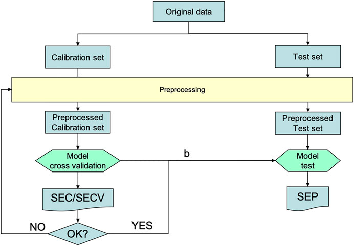
FIGURE 1. –The process of calibration (creating and adjusting the model) by cross validation, followed by its validation with a separate test set. “b” is the model calculated on the calibration set.

The model is adjusted by creating models with an increasing number of Latent Variables extracted from one set of individuals and observing the evolution of the differences between observed and predicted values for another set of individuals. This evolution can be followed by plotting the sum of squared residuals (RESS Residual Error Sum of Squares) or the square root of the mean sum of squares (RMSE). When this tuning is done with another single set of individuals (test-set validation), we have the SEV and RMSEV; when it is done by removing, with replacement, a few individuals from the data set (cross validation), we have the SECV and the RMSECV.

$\mathrm{RESS}={\displaystyle \sum }_1^{\mathit{n}}{\left(\widehat{{\mathit{y}}_{\mathit{i}}}-{\mathit{y}}_{\mathit{i}}\right)}^2(\mathrm{7a})$

$\mathrm{RMSEVorRMSECV}=\sqrt{\frac{{{\displaystyle \sum }}_1^{\mathit{n}}{\left(\widehat{{\mathit{y}}_{\mathit{i}}}-{\mathit{y}}_{\mathit{i}}\right)}^2}{\mathrm{n}}}(\mathrm{7b})$

Calculating the model and applying it on the entire dataset provides an estimation of Y (Ŷ), which is used to calculate the RMSEC:

$\mathrm{RMSEC}=\sqrt{\frac{{{\displaystyle \sum }}_1^{\mathit{n}}{\left(\widehat{{\mathit{y}}_{\mathit{i}}}-{\mathit{y}}_{\mathit{i}}\right)}^2}{\mathrm{n}-\left(\mathrm{nLVs}+1\right)}}(\mathrm{7c})$

The RMSEC is intended to estimate the standard deviation of the fitting error, σ. The division by [n-(k+1)] instead of n (the number of individuals) is intended to take into account the fact that the number of degrees of freedom for the estimate of σ is decreased by the inclusion of k Latent Variables plus the intercept. The use of this correction is valid in PCR regression, but subject to much criticism in the case of PLS where the Y matrix influences the calculation of the Latent Variables (Krämer and Sugiyama, 2011; Lesnoff et al., 2021). It is nevertheless sometimes used as a “naïve estimate of the RMSEC”.

The principle of cross-validation is presented in Figure 2. Blocks of individuals are removed from the dataset and are used as a test set while the remaining individuals form the calibration dataset to create models which are used to predict the values (Ŷ) for the test set individuals. The differences between the observed values (Y) and predicted values (Ŷ) are calculated for the different models. The test set individuals are then put back in the calibration dataset and another block of individuals is moved to be the test set. This process is repeated until all individuals have been used in the test set. If the size of the blocks is small (large number of blocks), the number of individuals tested each time is low and the number used to create the models is high. The limiting case is called Leave-One-Out Cross Validation (LOO-CV), where the number of blocks is equal to the total number of individuals. In this case, the result tends to be optimistic (small RMSECV) but simulates well the final model, because each prediction is made using a model calculated with a collection of samples close to that in the final model.

FIGURE 2

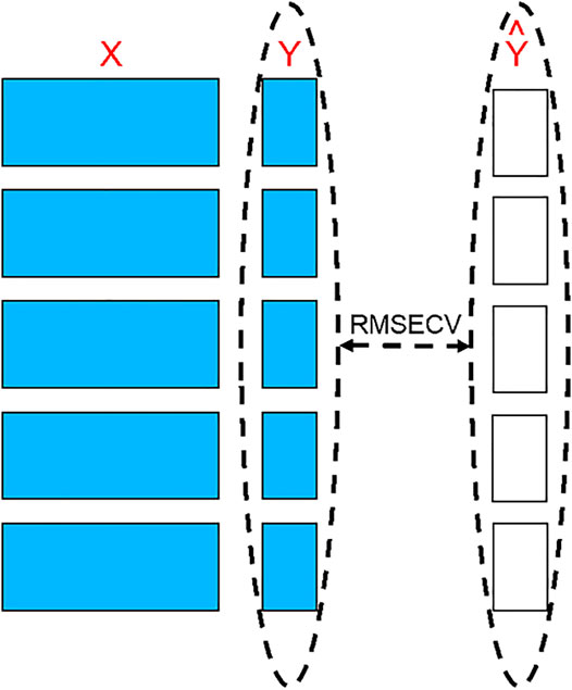
FIGURE 2. The principle of cross-validation. Blocks of individuals are removed from the dataset to be used as tests to measure the differences between their observed values and values predicted by the models created using the remaining individuals.

On the other hand, using large blocks allows us to better assess the predictive power of the model. In all cases, in order not to distort the results, it is necessary to ensure that repetitions of samples (e.g., triplicates) are kept together in the same block.

A fundamental hypothesis of theories on machine learning from empirical data assumes that the training and future datasets are generated from the same probability distribution (e.g., Faber, 1999; Denham, 2000; Vapnik, 2006; Lesnoff et al., 2021). Under this hypothesis, it is known that leave-one-out cross-validation has low bias but can have high variance for the prediction errors (i.e., variable prediction if the training set would be replicated) (Hastie et al., 2009). On the other hand, when K is smaller, cross-validation has lower variance but higher bias. Overall, five-or tenfold cross-validations are recommended as a good compromise between bias and variance (Hastie et al., p. 284).

There are many ways to build blocks, the choice being based on the organization of individuals in the matrix.

Consecutive Blocks: (1, 2, …, 10) (11, 12, …, 20) (21, 22, …, 30).

Venitian Blind: (1, 4, 7, …, 28) (2, 5, 8, …, 29) (3, 6, 9, …, 30).

Random Blocks

Predefined Blocks: for example, to manage measurement repetitions.

Figure 3 presents the evolution of the RMSECV (red circles) and the “naïve” RMSEC (blue squares) based on the number of Latent Variables used to create the prediction model. The “naïve” RMSEC, which quantifies the residual errors for the samples used to create the models, tends to zero. On the other hand, the RMSECV often has a minimum, more or less marked depending on the amount of noise in the data, which corresponds to the balance between information and noise, indicating the optimal number of Latent Variables.

FIGURE 3

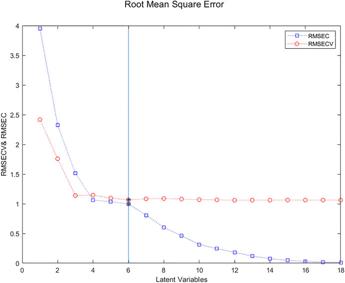
FIGURE 3. Evolution of the RMSECV (red circles) and the naïve RMSEC (blue squares) based on the number of Latent Variables used to create the prediction model. The minimum for 6 Latent Variables is clearly visible.

Although the minimum in the RMSECV curve is for 6 LVs, this value is not much lower than that for 3 LVs. Parsimony could imply retaining only 3 LVs. To visualize more clearly the point corresponding to the minimum of RMSECV, one can use a rule that says that, on the one hand, the prediction error (here estimated by RMSECV) should be close to the fitting error (here estimated by RMSEC) and on the other hand, the RMSEC curve may present a break. A way of implementing that rule is to plot the RMSECV against the RMSEC (Bissett, 2015).

In Figure 3 and many subsequent figures, a vertical line indicates the number of LVs resulting from a consensus found by the procedure we propose, i.e., by applying a PCA to the various very different criteria presented here.

To get a better indication of variability in the estimation of the optimal number of Latent Variables, repeated cross-validation is often used. In this case, several cross-validations are made with few blocks (here 2 blocks) containing randomly selected individuals each time. It is thus possible to calculate an average RMSECV and its variability (Figure 4).

FIGURE 4

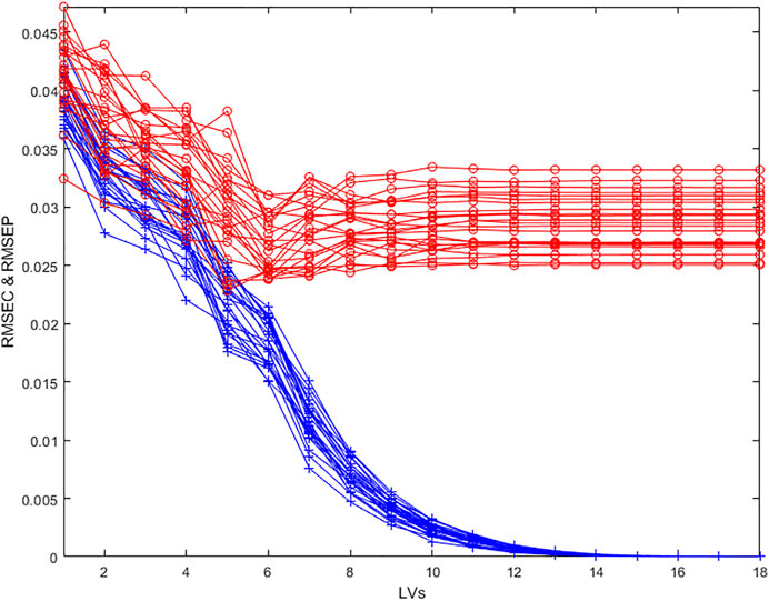
FIGURE 4. Evolution of the RMSECV (red circles) and naïve RMSEC (blue crosses) as a function of the number of Latent Variables in the model for 25 repetitions of a 2 random blocks cross validation.

Another related procedure is to plot the proportions of variability extracted from the Y vectors, R², for the calibration samples, and Q², for the samples removed during the cross validation, as a function of the number of Latent Variables. In Figure 5 one can see that the difference between R² and Q² is close to zero for from 4 to 6 LVs.

FIGURE 5

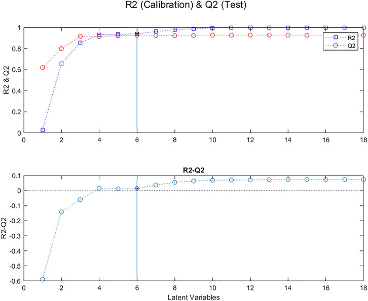
FIGURE 5. Evolution of R² (blue squares) and Q² (red circles), for “calibration” samples and “test” samples, respectively, as a function of the number of Latent Variables in the model; Evolution of the difference between R² and Q².

Other criteria can be calculated based on the values predicted by cross-validation.

Wold’s R criterion (Wold, 1978; Li et al., 2002) is given by:

$\mathrm{PRESS}\left(\mathrm{k}\right)={\displaystyle \sum }_1^{\mathit{n}}{\left(\widehat{{\mathit{y}}_{\mathit{i}}}-{\mathit{y}}_{\mathit{i}}\right)}^2(\mathrm{8a})$

$\mathrm{Wol}{\mathrm{d}}^{\text{'}}\mathrm{s}\mathrm{R}=\frac{\mathrm{PRESS}\left(2:\mathrm{k}\right)}{\mathrm{PRESS}\left(1:\mathrm{k}-1\right)}(\mathrm{8b})$

where PRESS(k) is the predicted residual sum of squares for k LVs; and Wold’s R is a vector of the ratios of successive PRESS values. The usual cutoff for Wold’s R criterion is when R is greater than unity. In Figure 6 it can be seen that the maximum R is at 6 LVs but the value is already greater than 1 for 3 LVs.

FIGURE 6

FIGURE 6. Evolution of Wold’s R; Osten’s criterion and Cattell’s Residual Percent Variance (RPV) criterion, as a function of the number of Latent Variables in the model.

More recently, Osten proposed the criterion (Osten, 1988), given by:

$\mathrm{Oste}{\mathrm{n}}^{\text{'}}\mathrm{s}\mathrm{F}\left(\mathrm{k}\right)=\frac{\mathrm{PRESS}\left(1:\mathrm{k}-1\right)-\mathrm{PRESS}\left(2:\mathrm{k}\right)}{\mathrm{PRESS}\left(2:\mathrm{k}\right)/\left(\mathrm{N}-\left(\mathrm{k}+1\right)\right)}(9)$

Figure 6 also shows that Osten’s F confirms the results for Wold’s R: F is less than 0 at 3 LVs but reaches a minimum at 6 LVs.

When doing a PCA, Cattell’s Residual Percent Variance (RPV) criterion (Cattell, 1966) assumes that the residual variance should level off, as in Figure 6, after a suitable number of factors have been extracted. RPV for the model with k LVs is given by:

$\mathrm{RPV}\left(\mathit{k}\right)=\frac{{{\displaystyle \sum }}_{\mathit{i}=\mathit{k}+1}^{\mathit{K}}{\lambda }_{\mathit{i}}}{{{\displaystyle \sum }}_{\mathit{i}=1}^{\mathit{K}}{\lambda }_{\mathit{i}}}(10)$

where ${\lambda }_i$ is the eigenvalue for the ith PC. Here, in the case of PLS, we have replaced the eigenvalues by the variances of the scores for each LV.

There are other methods, such as Mallow’s Cp (Mallows, 1973) and Akaike’s Information Criterion (AIC) (Akaike, 1969), that are commonly used to select the dimensionality of regression models, as an alternative to cross-validation (CV). However, the calculation of Cp and AIC requires the determination of the effective number of degrees of freedom of the model, which as mentioned above, is not straightforward in the case of PLS (Lesnoff et al., 2021). For that reason, these criteria will not be considered here.

Criteria based on other properties of the models

Cross-validation is sometimes difficult to perform, for example when there are many individuals and/or variables, so the calculation time can be excessive. And even when the calculation is feasible, one does not always observe a clear minimum in the RMSECV curve (as in Figure 3) or maximum in the Q² curve (as in Figure 5), which makes it difficult to choose the number of LVs.

As well, as indicated by Wiklund et al. (2007) CV handles “the available data economically, but like any data-based statistical test gives an interval of results and hence sometimes gives either an under-fit or an over-fit, that is they reach the minimum RMSEV for a lower or higher model rank than would be achieved using an infinitely large independent validation set”. They also stressed the fact that “One area where CV works poorly both for PLS and PCR is design of experiments, where exclusion of data has large consequences for modeling”. To solve these problems, they proposed carrying out permutation tests on the Y vector and then comparing the correlations between the scores of each latent variable and the true Y vector with the correlations between the scores obtained for the permuted Ys and the corresponding true Ys.

It should be noted that all these criteria are based on comparing the observed and predicted Y vectors. It could therefore be helpful to use other criteria based on entirely different characteristics of the models to facilitate the choice of the number of latent variables.

We will now see a set of such complementary methods, based on the characteristics of the regression coefficients vectors, b, and on the characteristics of the X matrix after each deflation.

Characteristics of the Regression Coefficients Vectors, b

As the number of Latent Variables used to calculate the regression coefficients vector, b, increases, more and more noise is included. When the X matrix contains structured signals, such as the near infrared spectra in Supplementary Figure S1, b coefficients are initially structured and gradually become random, as can be seen in Figure 7.

FIGURE 7

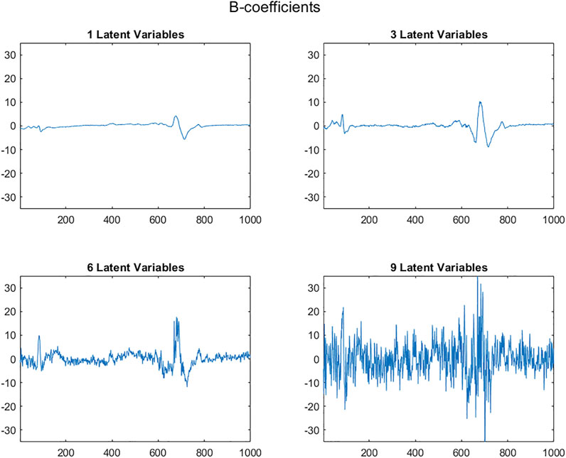
FIGURE 7. PLS regression coefficient vectors, b, based on 1, 3, 6 and 9 Latent Variables plotted with a constant ordinate scale (abscissa: variable numbers).

In the case of b-vectors calculated from structured signals in the rows of the X matrix, a “signal-to-noise ratio” can be calculated using the Durbin-Watson (DW) criterion (Durbin and Watson, 1971; Rutledge and Barros, 2002). This criterion is given by:

$\mathbf{DW}=\frac{{{\displaystyle \sum }}_{\mathit{i}=2}^{\mathit{n}}{\left({\mathit{b}}_{\mathit{i}} -{\mathit{b}}_{\mathit{i}-1}\right)}^2}{{{\displaystyle \sum }}_{\mathit{i}=1}^{\mathit{n}}{\mathit{b}}_{\mathit{i}}^{\mathrm{2}}}(11)$

where b_i and b_(i-1) are the values for successive points in a series of b-coefficients values. DW is close to zero if there is a strong correlation between successive values. On the other hand, if there is a low correlation (i.e., a random distribution), the value of DW tends to 2.0. DW can therefore be used to characterize the degree of correlation between successive points, and thus give an objective measure of the non-random behavior of the b coefficients vectors. However, if the noise in the data has been reduced by smoothing, the transition will not be as clear and DW will not increase as much.

Figure 8 shows the evolution of DW calculated for a succession of regression coefficients vectors, as a function of the increasing number of LVs used in the PLS model. It is clear that there is a very sudden increase in DW after 6 LVs.

FIGURE 8

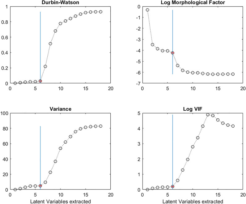
FIGURE 8. Evolution of the Durbin-Watson (DW) criterion; the log of the Morphological Factor; the Variance; the Variance Inflation Factor (VIF) calculated on the regression vectors, b, as a function of the number of Latent Variables in the PLS models.

The Morphological Factor (MF) (Wang et al., 1996) is based on the same phenomenon as the DW criterion, noisy vectors are less structured than non-noisy vectors. On the other hand, the mathematical principle is different:

$\mathrm{MF}\left(\mathbf{b}\right)=\Vert \mathbf{b}\Vert \mathrm{/}\left(\Vert \mathbf{MO}\left(\mathbf{b}\right)\Vert .\mathrm{ZCP}\left(\mathbf{MO}\left(\mathbf{b}\right)\right)\right)(\mathrm{12a})$

$\mathbf{MO}\left(\mathbf{b}\right)={\mathbf{b}}_{\mathbf{i+1}}-{\mathbf{b}}_{\mathbf{i}}\left(\mathrm{for}\mathrm{i=1,2,}\dots \mathrm{n-1}\right)(\mathrm{12b})$

where b is a vector of regression coefficients; MO(b) the vector of differences in intensity between successive points in b; ZCP (MO(b)) the number of times MO(b) changes signs, and the operator ||o|| is the Euclidian norm.

In the case of a noisy vector, MO(b) will contain bigger values and there will be more sign changes than in the case of a smooth vector, resulting in lower MF values. Figure 8 shows the evolution of MF as a function of the number of Latent Variables extracted. The log of MF evolves in a similar way to the DW criterion with a decrease after 6 Latent Variables.

In the case of an X matrix that does not contain structured signals (e.g., physical-chemical data or mass spectra) DW or MF should not be used. But other characteristics of the regression vectors can be used instead.

It can be seen that the range of b vector values initially remains relatively stable, but beyond a certain number of LVs, the b-coefficient values increase enormously (Figure 7). By plotting the variance of the regression vectors it is possible to see the point at which this phenomenon appears (Figure 8) for both structured and non-structured data matrices. This is also true for the standard deviation or the norm of the vectors.

The Variance Inflation Factor of a variable i in a matrix X (VIFi) (Marquardt, 1970; Ferré, 2009) is equal to the inverse of (1-Ri²), where Ri² is the coefficient of determination of the regression between all the other predictor variables in the matrix and the variable i. VIFi quantifies the degree to which that variable can be predicted by all the others. The closer the Ri² value to 1, the higher the multicollinearity with independent variable i and the higher the value of VIFi.

As the number of LVs included in a regression model increases, the structure of the b-coefficients vectors changes due to the inclusion of more sources of variability, initially corresponding to information, and later to noise. There are initially significant changes in the b coefficient vectors, due to the fact that the loadings are very different, reflecting different sources of information. Subsequent loadings correspond more and more to noise and change less the shape of the b-vectors.

It can therefore be interesting to quantify the correlations between the columns of a matrix B containing vectors of b-coefficients calculated with increasing numbers of LVs.

To detect the number of LVs at which point the multi-collinearities increase, we can plot the VIF values of the b-coefficient vectors as a function of the number of LVs. In Figure 8, we see that the VIF values remain low up to 6 LVs, and then increase.

In a way similar to the Random_ICA method (Kassouf et al., 2018), one can study whether similar b-coefficients vectors are extracted from two random subsets of the X and Y matrices. PLS regressions are performed with increasing numbers of LVs on the two subsets. Too many LVs have been extracted when there is no longer a strong correlation between the pair of b-coefficients vectors. To avoid the possibility of a bias being introduced by a particular distribution of the rows into the two blocks, the whole procedure is repeated k times resulting in different sets of blocks, producing a broader perspective for the selection of the number of LVs (Figure 9).

FIGURE 9

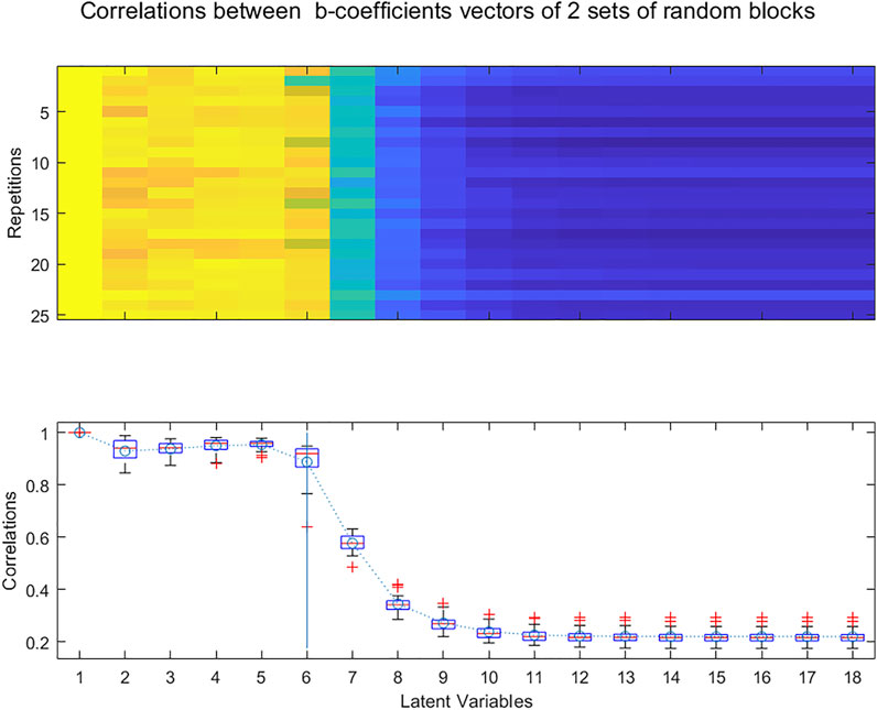
FIGURE 9. Evolution of the correlations between b-coefficients calculated for 25 randomly selected pairs of subsets of samples for increasing numbers of Latent Variables.

Structure of the X Matrix After Each Deflation Step.

Most multivariate analysis methods contain a deflation step where the contribution of each Latent Variables is removed from the matrix before extracting the next Latent Variables. This is true for PCA, PCR and PLS. This process of deflation means that the rows in the deflated matrices contain less and less information and more and more noise. As well, since the remaining variability corresponds more and more to Gaussian noise, the distribution of individuals in the space of the variables gradually approaches that of a hypersphere.

Several criteria can be used to characterize the evolution of the signal/noise ratios in the rows and the sphericity of the deflated matrices so as to determine when all the interesting information has been removed.

Again, the DW criterion can be used, this time to measure the signal-to-noise ratio in each row of the matrix following the successive deflations. Figure 10 shows the evolution of the distribution of DW values calculated as in Equation 13, for each row of the X matrix, as a function of the number of Latent Variables extracted.

$\mathbf{DW}=\frac{{{\displaystyle \sum }}_{\mathit{i}=2}^{\mathit{n}}{\left({\mathit{x}}_{\mathit{i}} -{\mathit{x}}_{\mathit{i}-1}\right)}^2}{{{\displaystyle \sum }}_{\mathit{i}=1}^{\mathit{n}}{\mathit{x}}_{\mathit{i}}^2}(13)$

FIGURE 10

FIGURE 10. Evolution of the Durbin-Watson (DW) criterion; the Morphological Factor; the Variance calculated for each row of the X matrix during deflation and the log of the VIF for all X-matrix variables after each deflation.

There is a sharp increase in the median value and interquartile interval when 5 latent variables are extracted. The heatmap and boxplot show that not all rows (samples) evolve in the same way, some becoming noisy later than most. This is reflected in the size of the boxplots of the DW values and also in the standard deviation of the values.

As with the DW criterion, the Morphological Factor can be calculated for each row of the matrix after deflation. Figure 10 also shows the evolution of the distribution of the MF values, as a function of the number of Latent Variables extracted. The values stabilize with the elimination of 6 Latent Variables.

For non-structured data, the variance (or the standard deviation or the Norm) of the matrix rows can be used (Figure 10).

As the X-matrix is deflated, the sources of variability corresponding to information are eliminated, leaving behind only random noise, so that there are less and less correlations between the variables in the deflated X-matrix. To detect the moment when there are no more multi-collinearities between the variables, we can do linear regressions between each variable and all the others and then examine the corresponding R² for all successive models. If the R² of a variable is close to 1, there is still a linear relationship between this variable and the others.

The VIF is equal to the inverse of (1-R²). If the VIF of a variable is greater than 4, there may be multi-collinearities; if the VIF is greater than 10, there are significant multi-collinearities.

To determine whether all information has been eliminated from the X-matrix, the VIFs of all the variables can be plotted as a function of the number of LVs extracted, as in Figure 10, where only a few variables still have high VIFs after eliminating 6 LVs.

As the X-matrix is deflated, the dispersion of the samples in the reduced multivariate space tends to become spherical, as all the directions of non-random dispersion are progressively removed. Sphericity tests can therefore be applied to the deflated matrices to determine how many LVs are required to remove all interesting dispersions.

Bartlett’s test for Sphericity (Bartlett, 1951) compares a matrix of Pearson correlations with the identity matrix. The null hypothesis is that the variables are not correlated. If there is redundancy between variables, it can be interesting to proceed with the multivariate analysis. The formula is given by:

${\mathit{\chi }}^{\mathbf{2}}\mathbf{=}\mathbf{-}\mathbf{\left[}\mathbf{\left(}\mathit{n}\mathbf{-}\mathbf{1}\mathbf{\right)}\mathbf{-}\mathbf{\left(}\mathbf{2}\mathit{k}+\mathbf{5}\mathbf{\right)}\mathbf{6}\mathbf{\right]}\mathit{*log}\mathbf{\left|}\mathbf{R}\mathbf{\right|}(14)$

where:

n is the number of observations, k the number of variables, and R the correlation matrix of the data in X. |R| is the determinant of R.

Bartlett’s test in Figure 11 shows that the deflated matrices are very non-spherical until after 6 LVs have been removed.

FIGURE 11

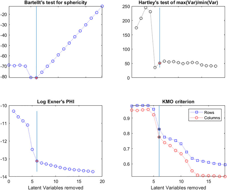
FIGURE 11. Evolution of Bartlett’s test for Sphericity; Hartley’s F-test; the Log of Exner’s Phi criterion and the KMO criterion for X-matrix rows and columns, as a function of the number of Latent Variables in the model.

Similarly, Hartley and Cochran proposed F-tests based on the ratio of the maximum variance/minimum variance (Hartley, 1950) and the maximum variance/mean variance (Cochran, 1941), respectively. The Hartley criterion in Figure 11 shows that the deflated matrices are very spherical once 5 LVs are removed.

Exner proposed the Ψ criterion (Exner, 1966; Kindsvater et al., 1974) as a measure of fit of a set of predicted data to a set of experimental data, given by the equation:

$\mathit{\psi }=\sqrt{\left[\frac{{{\displaystyle \sum }}_{\mathit{i}=1}^{\mathit{nc}}\mathit{ }{\left({\mathit{X}}_{\mathit{i}}-\widehat{{\mathit{X}}_{\mathit{i}}}\right)}^2}{{{\displaystyle \sum }}_{\mathit{i}=1}^{\mathit{nc}}{\left({\mathit{X}}_{\mathit{i}}-\overline{\mathit{X}}\right)}^2}\frac{\mathit{nc}}{\mathit{nc}-\mathit{k}}\right]}(15)$

where ${\text{X}}_{\text{i}}$ is a data point in the matrix, ${\widehat{\text{X}}}_{\text{i}}$ is that data point reproduced using k LVs, n and c are the number of rows and columns in the data matrix and $\overline{\text{X}}$ is the grand mean of X.

Here Exner’s criterion (Figure 11) is calculated between the original X matrix and each successive deflated matrix to determine at what point there is no longer any similarity between them.

The KMO (Kaiser-Meyer-Olkin Measure of Sampling Adequacy) criterion (Kaiser, 1970; Kaiser, 1974) was developed to determine whether it was useful to conduct a multivariate analysis of a data matrix. For example, if the variables are uncorrelated, it is no use to do a PCA.

The KMO index is given by:

$\mathbf{KMO=}\frac{{\displaystyle \sum _{\mathit{i}}{\displaystyle \sum _{\mathit{j}\ne \mathit{i}}{{\displaystyle r}}_{i\mathit{j}}^2}}}{{\displaystyle \sum _{\mathit{i}}{\displaystyle \sum _{\mathit{j}\ne \mathit{i}}{{\displaystyle r}}_{\mathit{ij}}^2}}+{\displaystyle \sum _{\mathit{i}}{\displaystyle \sum _{\mathit{j}\ne \mathit{i}}{{\displaystyle \mathit{a}}}_{\mathit{ij}}^2}}}(\mathrm{16a})$

where r_ij is the correlation between variables i and j, and a_ij is the partial correlation, defined as:

${\mathit{a}}_{\mathit{ij}}=\frac{{\mathit{v}}_{\mathit{ij}}}{\sqrt{{\mathit{v}}_{\mathit{ij}}+{\mathit{v}}_{\mathit{ij}}}}(\mathrm{16b})$

ν_ij being an element of the inverse of the correlation matrix (ν_ij = r_ij ⁻¹).

The value of the KMO index varies between 0 (no correlation between variables, thus useless to do a multivariate analysis) and 1 (correlated variables, thus useful to do a multivariate analysis). A KMO value of 0.5 is usually considered the cutoff point below which there is no interest in doing a multivariate analysis. Here this index was calculated for the variables (columns) and for the individuals (rows) in each matrix. We can see (Figure 11) that the values are close to 1 until 6 LVs are removed from the matrix and that there is a second decrease after removing 11 LVs. This means that much of the information shared by the original variables and individuals has been removed by 6 LVs, but there is still some present to a lesser extent up to 11 LVs.

In 1977, Malinowski (1977a) developed the idea that there were two types of Factors (or Latent Variables) “a primary set which contains the true factors together with a mixture of error and a secondary set which consists of pure error”. He also showed that there were three types of errors: RE, real error; XE, extracted error; and IE, Imbedded error, which can be calculated “from a knowledge of the secondary eigenvalues, the size of the data matrix, and the number of factors involved”, the secondary eigenvalues being those associated with pure noise.

He considered that if k, the number of LVs associated with the “pure data” is known, the real error is the difference between the pure data and the raw data, that is the Residual Standard Deviation (RSD) given by:

$\mathit{RE}=\mathit{RSD}=\sqrt{\left[\frac{{{\displaystyle \sum }}_{\mathit{i}=\mathit{k}+1}^{\mathit{c}}\mathit{ }{\mathit{\lambda }}_{\mathit{i}}}{\mathit{n}\left(\mathit{c}-\mathit{k}\right)}\right]}(17)$

where, n and c are the respective number of rows and columns in the data matrix; k the number of factors used to reproduce the data; and λi is the ith eigenvalue.

He stressed that “it was assumed that n > c. If the reverse is true, i.e., n < c, then n and c must be interchanged in these equations”.

He also proposed that the imbedded error (IE) is the difference between the pure data and the data approximated by the multivariate decomposition:

$\mathit{IE}=\sqrt{\frac{\mathit{k}}{\mathit{c}}}\mathit{RSD}(18)$

and that the extracted error (XE) is the difference between the data approximated by the multivariate decomposition and the raw data:

$\mathit{XE}=\sqrt{\frac{\mathit{c}-\mathit{k}}{\mathit{c}}}\mathit{RSD}(19)$

Malinowski then proposed another empirical criterion to determine the number of Latent Variables in a data matrix (Malinowski, 1977b). This indicator function (IND) is closely related to the error functions described above:

$\mathit{IND}=\frac{\mathit{RSD}}{{\left(\mathit{c}-\mathit{k}\right)}^2}(20)$

As can be seen in Figure 12, a plot of these criteria as a function of k, the number of LVs, can help to distinguish “pure data” from “error data”.

FIGURE 12

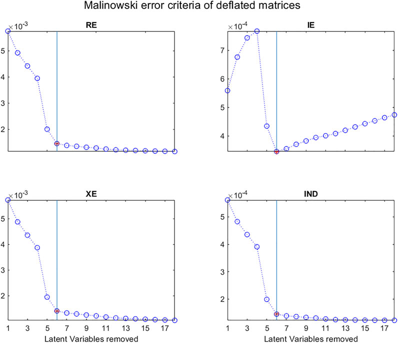
FIGURE 12. Evolution of the 4 criteria proposed by Malinowski after each deflation.

Several criteria have been proposed to estimate the correlation between matrices. Here 3 of them (Dray, 2008) will be used to compare the original X matrix with each deflated matrix, the assumption being that these correlations will decrease as the information is being removed.

The RV coefficient (Escoufier, 1973; Robert and Escoufier 1976) is a measurement of the closeness between two matrices and is defined by:

$\mathit{RV}=\frac{\mathit{trace}\left({\mathit{X}}_1{\mathit{X}}_1^{\mathit{T}}{\mathit{X}}_{\mathit{k}}{\mathit{X}}_{\mathit{k}}^{\mathit{T}}\right)}{\sqrt{\mathit{trace}\left({\mathit{X}}_1^{\mathit{T}}{\mathit{X}}_1{\mathit{X}}_1^{\mathit{T}}{\mathit{X}}_1\right)\mathit{trace}\left({\mathit{X}}_{\mathit{k}}^{\mathit{T}}{\mathit{X}}_{\mathit{k}}{\mathit{X}}_{\mathit{k}}^{\mathit{T}}{\mathit{X}}_{\mathit{k}}\right)}}(21)$

In our case, X₁ is the original matrix, X_k is the deflated matrix after removing k LVs.

The numerator of the RV coefficient is the co-inertia criterion (COI) (Dray et al., 2003) which is also a measurement of the link between the two matrices:

$\mathit{COI}=\mathit{trace}\left({\mathit{X}}_1{\mathit{X}}_1^{\mathit{T}}{\mathit{X}}_{\mathit{k}}{\mathit{X}}_{\mathit{k}}^{\mathit{T}}\right)(22)$

According to Ramsay et al. (1984) and Kiers et al. (1994), the most common matrix correlation coefficient is the ‘inner product’ matrix correlation coefficient, which we will call RIP, defined as:

$\mathit{RIP}=\frac{\mathit{trace}\sqrt{\left({\mathit{X}}_1^{\mathit{T}}{\mathit{X}}_{\mathbf{k}}\right)}}{\sqrt{\mathit{trace}\left({\mathit{X}}_1^{\mathit{T}}{\mathit{X}}_1\right)\mathit{trace}\left({\mathit{X}}_{\mathit{k}}^{\mathit{T}}{\mathit{X}}_{\mathit{k}}\right)}}(23)$

Figure 13 shows the evolution of these 3 measures of the correlation between the original X matrix and the matrices after deflation.

FIGURE 13

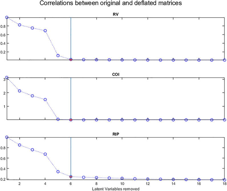
FIGURE 13. Evolution of RV, COI and RIP of the X-matrix after each deflation.

Consensus Number of Latent Values

Given all the criteria that can be calculated, one needs to find a consensus value for the number of LVs to retain in the PLS regression model. Some criteria (RMSEC and RMSECV in Figure 3; R² and Q² in Figure 5; Wold’s R, Osten’s F and Cattell’s RPV in Figure 6) characterize the proximity of the predicted values to the observed values, but they can be subject to errors due to the particular choice of the calibration and test sets. Others characterize the regression coefficients (B-DW, B_Morph, B_VIF in Figure 8) which should not be excessively noisy or of too high a magnitude (B_Var in Figure 8). As well, similar B-coefficients vectors should be extracted from subsets of the data matrix (mean of the correlations between regression coefficients vectors in Figure 9). Still others characterize the noisy structure of the residual variability in the deflated matrices (mean and standard deviations of DW_X, Morph_X, Var_X and VIF_X in Figure 10 as well as Malinowski’s RE, IE, XE and IND in Figure 12).

These deflated matrices should also tend towards a spherical structure (Bartlett_X, Hartley_X, Exner_X, KMO_X_rows, KMO_X_columns in Figure 11). As well, as successive components are removed, the correlations between the original matrix and the deflated matrices should decrease (RV, COI and RIP in Figure 13).

To create a consensus of all these different types of information, we propose to apply a Principal Components Analysis to the various criteria.

All the criteria were concatenated so that each row corresponded to a number of Latent Values and the columns contained the criteria. Criteria such as DW were used as is while for criteria like RMSECV the inverse was used, so that in all cases, earlier LVs are associated with lower values.

The matrix was then z-transformed by subtracting the column means and dividing by the column standard deviations.

The resulting PC1-PC2 Scores plot and Loadings plot are presented in Figure 14.

FIGURE 14

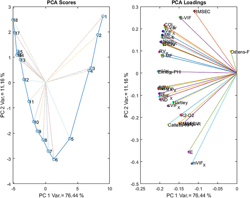
FIGURE 14. Plot of PC1-PC2 scores and loadings after applying a PCA to the standardized criteria.

The scores plot shows a clear evolution from low dimensionality models to high dimensionality along PC1, reflecting the increase in all values as the number of LVs increases. The evolution along PC2 corresponds to another phenomenon since the scores are highly positive for both small and large numbers of LVs, with a very clear negative minimum for a model at 6 LVs. The loadings plots shows an opposition between RMSEC, COI, std_Var_X, std_Morph_X and most of the criteria based on the B-coefficients vectors on the positive side; while mean_VIF_X, IE, RMSECV, Wold’s R, Cattell’s RPV, R2-Q2 and most of the criteria based on the deflated X matrices are on the negative side. This contrast between the criteria based on the B-coefficients vectors and those based on the deflated X matrices shows their complementary nature.

Only the first 2 PCs are presented as the following scores (corresponding to models with increasing numbers of LVs) did not have any interpretable structure.

Conclusion

PLS regression is a high-performance calibration and prediction method to link predictive X-variables to the Y-variables to be predicted, even when variables are highly correlated and in very large numbers.

However, adjusting the number of latent variables in the model is crucial. This adjustment should be done on the basis of several criteria.

To do this, various methods can be used:

The most common method is to observe the evolution of calibration errors (RMSEC) and validation or cross validation errors (RMSEV or RMSECV); One can also examine the evolution of the vectors of regression coefficients. This also provides information on the role of the variables or spectral components in the model; Finally, the evolution in the structure of the rows and columns as well as the sphericity of the X-matrix after each deflation step, can be examined.

To do this we have proposed applying a Principal Components Analysis to a collection of criteria characterizing the different aspects of models obtained with increasing numbers of Latent Variables. The set of criteria used in the present study is far from exhaustive, and the efficacy of the method may even be improved by including others.

Matlab function to calculate most of the non-trivial criteria are to be found at: https://github.com/DNRutledge/LV_Criteria.

Data Availability Statement

The data analyzed in this study is subject to the following licenses/restrictions: Interested readers should contact the authors of the article cited as producers of the data. Requests to access these datasets should be directed to nathalie.dupuy@imbe.fr.

Author Contributions

DR: Conception, calculations, writing J-MR: Corrections, calculations, writing ML: Corrections, calculations, writing.

Conflict of Interest

The authors declare that the research was conducted in the absence of any commercial or financial relationships that could be construed as a potential conflict of interest.

Publisher’s Note

All claims expressed in this article are solely those of the authors and do not necessarily represent those of their affiliated organizations, or those of the publisher, the editors, and the reviewers. Any product that may be evaluated in this article, or claim that may be made by its manufacturer, is not guaranteed or endorsed by the publisher.

Supplementary Material

The Supplementary Material for this article can be found online at: https://www.frontiersin.org/articles/10.3389/frans.2021.754447/full#supplementary-material

References

Akaike, H. (1969). Fitting Autoregressive Models for Prediction. Ann. Inst. Stat. Math. 21, 243–247. doi:10.1007/BF02532251

CrossRef Full Text | Google Scholar

Bartlett, M. S. (1951). The Effect of Standardization on A Χ2 Approximation in Factor Analysis. Biometrika 38 (3/4), 337–344. doi:10.1093/biomet/38.3-4.337

CrossRef Full Text | Google Scholar

Bissett, A. C. (2015). Improvements to PLS Methodology, PhD. Manchester: University of Manchester. Available at: http://www.manchester.ac.uk/escholar/uk-ac-man-scw:261814.

Google Scholar

Cattell, R. B. (1966). The Scree Test for the Number of Factors. Multivariate Behav. Res. 1 (2), 245–276. doi:10.1207/s15327906mbr0102_10

PubMed Abstract | CrossRef Full Text | Google Scholar

Cochran, W. G. (1941). The Distribution of the Largest of a Set of Estimated Variances as a Fraction of Their Total. Ann. Eugenics 11 (1), 47–52. doi:10.1111/j.1469-1809.1941.tb02271.x

CrossRef Full Text | Google Scholar

Denham, M. C. (2000). Choosing the Number of Factors in Partial Least Squares Regression: Estimating and Minimizing the Mean Squared Error of Prediction. J. Chemometrics 14 (4), 351–361. doi:10.1002/1099-128X(200007/08)14:4<351::AID-CEM598>3.0.CO;2-Q

CrossRef Full Text | Google Scholar

Dray, S., Chessel, D., Chessel, D., and Thioulouse, J. (2003). Co-inertia Analysis and the Linking of Ecological Data Tables. Ecology 84, 3078–3089. doi:10.1890/03-0178

CrossRef Full Text | Google Scholar

Dray, S. (2008). On the Number of Principal Components: A Test of Dimensionality Based on Measurements of Similarity between Matrices. Comput. Stat. Data Anal. 52, 2228–2237. doi:10.1016/j.csda.2007.07.015

CrossRef Full Text | Google Scholar

Durbin, J., and Watson, G. S. (1971). Testing for Serial Correlation in Least Squares Regression. III. Biometrika 58, 1–19. doi:10.2307/2334313

CrossRef Full Text | Google Scholar

Escoufier, Y. (1973). Le traitement des variables vectorielles. Biometrics 29, 751–760. doi:10.2307/2529140

CrossRef Full Text | Google Scholar

Exner, O. (1966). Additive Physical Properties. I. General Relationships and Problems of Statistical Nature. Collect. Czech. Chem. Commun. 31, 3222–3251. doi:10.1135/cccc19663222

CrossRef Full Text | Google Scholar

Faber, N. M. (1999). Estimating the Uncertainty in Estimates of Root Mean Square Error of Prediction: Application to Determining the Size of an Adequate Test Set in Multivariate Calibration. Chemometrics Intell. Lab. Syst. 49 (1), 79–89. doi:10.1016/S0169-7439(99)00027-1

CrossRef Full Text | Google Scholar

Ferré, J. (2009). “Regression Diagnostics,” in Comprehensive Chemometrics. Editors S. D. Brown, R. Tauler, and B. Walczak (Amsterdam: Elsevier), 33–89. 9780444527011. doi:10.1016/B978-044452701-1.00076-4

CrossRef Full Text | Google Scholar

Galtier, O., Dupuy, N., Le Dréau, Y., Ollivier, D., Pinatel, C., Kister, J., et al. (2007). Geographic Origins and Compositions of virgin Olive Oils Determinated by Chemometric Analysis of NIR Spectra. Analytica Chim. Acta 595, 136–144. doi:10.1016/j.aca.2007.02.033

CrossRef Full Text | Google Scholar

Hartley, H. O. (1950). The Maximum F-Ratio as a Short-Cut Test for Heterogeneity Op Variance. Biometrika 37, 308–312. doi:10.1093/biomet/37.3-4.308

PubMed Abstract | CrossRef Full Text | Google Scholar

Hastie, T., Tibshirani, R., and Friedman, J. (2009). The Elements of Statistical Learning: Data Mining, Inference, and Prediction. 2nd ed. New York: Springer.

Google Scholar

Kaiser, H. F. (1970). A Second Generation Little Jiffy. Psychometrika 35, 401–415. doi:10.1007/BF02291817

CrossRef Full Text | Google Scholar

Kaiser, H. F. (1974). An index of Factorial Simplicity. Psychometrika 39, 31–36. doi:10.1007/BF02291575

CrossRef Full Text | Google Scholar

Kassouf, A., Jouan-Rimbaud Bouveresse, D., and Rutledge, D. N. (2018). Determination of the Optimal Number of Components in Independent Components Analysis. Talanta 179, 538–545. doi:10.1016/j.talanta.2017.11.051

PubMed Abstract | CrossRef Full Text | Google Scholar

Kiers, H. A. L., Cléroux, R., and Ten Berge, J. M. F. (1994). Generalized Canonical Analysis Based on Optimizing Matrix Correlations and a Relation with IDIOSCAL. Comput. Stat. Data Anal. 18, 331–340. doi:10.1016/0167-9473(94)90067-1

CrossRef Full Text | Google Scholar

Kindsvanter, J. H., Weiner, P. H., and Klingen, T. J. (1974). Correlation of Retention Volumes of Substitutued Carboranes with Molecular Properties in High Pressure Liquid Chromatography Using Factor Analysis. Anal. Chem. 46, 982–988. doi:10.1021/ac60344a032

CrossRef Full Text | Google Scholar

Krämer, N., and Sugiyama, M. (2011). The Degrees of Freedom of Partial Least Squares Regression. J. Am. Stat. Assoc. 106 (494), 697–705. doi:10.1198/jasa.2011.tm10107

CrossRef Full Text | Google Scholar

Lesnoff, M., Roger, J. M., and Rutledge, D. N. (2021). Monte Carlo Methods for Estimating Mallows's Cp and AIC Criteria for PLSR Models. Illustration on Agronomic Spectroscopic NIR Data. J. Chemometrics. doi:10.1002/cem.3369

CrossRef Full Text | Google Scholar

Li, B., Morris, J., and Martin, E. B. (2002). Model Selection for Partial Least Squares Regression. Chemometrics Intell. Lab. Syst. 64, 79–89. doi:10.1016/S0169-7439(02)00051-5

CrossRef Full Text | Google Scholar

Malinowski, E. R. (1977b). Determination of the Number of Factors and the Experimental Error in a Data Matrix. Anal. Chem. 49 (4), 612–617. doi:10.1021/ac50012a027

CrossRef Full Text | Google Scholar

Malinowski, E. R. (1977a). Theory of Error in Factor Analysis. Anal. Chem. 49 (4), 606–612. doi:10.1021/ac50012a02710.1021/ac50012a026

CrossRef Full Text | Google Scholar

Mallows, C. L. (1973). Some Comments onCp. Technometrics 15 (4), 661–675. doi:10.1080/00401706.1973.10489103

CrossRef Full Text | Google Scholar

Marquardt, D. W. (1970). Generalized Inverses, Ridge Regression, Biased Linear Estimation, and Nonlinear Estimation. Technometrics 12 (3), 591–612. doi:10.1080/00401706.1970.1048869910.2307/1267205

CrossRef Full Text | Google Scholar

Meloun, M., Čapek, J., Mikšı́k, P., and Brereton, R. G. (2000). Critical Comparison of Methods Predicting the Number of Components in Spectroscopic Data. Analytica Chim. Acta 423, 51–68. doi:10.1016/S0003-2670(00)01100-4

CrossRef Full Text | Google Scholar

Osten, D. W. (1988). Selection of Optimal Regression Models via Cross-Validation. J. Chemometrics 2, 39–48. doi:10.1002/cem.1180020106

CrossRef Full Text | Google Scholar

Ramsay, J. O., Ten Berge, J., and Styan, G. P. H. (1984). Matrix Correlation. Psychometrika 49, 403–423. doi:10.1007/BF02306029

CrossRef Full Text | Google Scholar

Robert, P., and Escoufier, Y. (1976). A Unifying Tool for Linear Multivariate Statistical Methods: The RV- Coefficient. Appl. Stat. 25, 257–265. doi:10.2307/2347233

CrossRef Full Text | Google Scholar

Rutledge, D. N., and Barros, A. S. (2002). The Durbin-Watson Statistic as a Morphological Estimator of Information Content. Analytica Chim. Acta 446, 279–294. doi:10.1016/S0003-2670(01)01555-0

CrossRef Full Text | Google Scholar

Vapnik, V. (2006). Estimation of Dependences Based on Empirical Data. 2nd ed. New York: Springer.

Google Scholar

Wang, J.-H., Liang, Y.-Z., Jiang, J.-H., and Yu, R.-Q. (1996). Local Chemical Rank Estimation of Two-Way Data in the Presence of Heteroscedastic Noise: A Morphological Approach. Chemometrics Intell. Lab. Syst. 32, 265–272. doi:10.1016/0169-7439(95)00072-0

CrossRef Full Text | Google Scholar

Wiklund, S., Nilsson, D., Eriksson, L., Sjöström, M., Wold, S., and Faber, K. (2007). A Randomization Test for PLS Component Selection. J. Chemometrics 21, 427–439. doi:10.1002/cem.1086

CrossRef Full Text | Google Scholar

Wold, S. (1978). Cross-Validatory Estimation of the Number of Components in Factor and Principal Components Models. Technometrics 20 (4), 397–405. doi:10.2307/126763910.1080/00401706.1978.10489693

CrossRef Full Text | Google Scholar