 Leah D. Pfeifer
 Milani W. Patabandige
 Heather Desaire
- Department of Chemistry, University of Kansas, Lawrence, KS, United States
Applying machine learning strategies to interpret mass spectrometry data has the potential to revolutionize the way in which disease is diagnosed, prognosed, and treated. A persistent and tedious obstacle, however, is relaying mass spectrometry data to the machine learning algorithm. Given the native format and large size of mass spectrometry data files, preprocessing is a critical step. To ameliorate this challenge, we sought to create an easy-to-use, continuous pipeline that runs from data acquisition to the machine learning algorithm. Here, we present a start-to-finish pipeline designed to facilitate supervised and unsupervised classification of mass spectrometry data. The input can be any ESI data set collected by LC-MS or flow injection, and the output is a machine learning ready matrix, in which each row is a feature (an abundance of a particular m/z), and each column is a sample. This workflow provides automated handling of large mass spectrometry data sets for researchers seeking to implement machine learning strategies but who lack expertise in programming/coding to rapidly format the data. We demonstrate how the pipeline can be used on two different mass spectrometry data sets: 1) ESI-MS of fingerprint lipid compositions acquired by direct infusion and, 2) LC-MS of IgG glycopeptides. This workflow is uncomplicated and provides value via its simplicity and effectiveness.
1 Introduction
The value of machine learning is best realized with large amounts of data; thus, a prime data type for machine learning is generated by mass spectrometry experiments. Applying machine learning strategies to mass spectrometry has yielded many advancements in the realm of human health; early detection of cancer, (Huang et al., 2020; Manzi et al., 2021; Sho et al., 2021), clinical decision support, (Acharjee et al., 2017; Zhang et al., 2020a; Mészáros et al., 2020; Sho et al., 2021), monitoring treatment response, (Zhang et al., 2020b; Hua et al., 2020), facilitating the discovery of novel drugs (Barthélemy et al., 2020; van Oosten and Klein, 2020), identifying microbial strains and screening for antibiotic resistance (Weis et al., 2020), and classifying single-cell types (Xie et al., 2020).
A significant challenge, however, is the reproducible and comprehensive transfer of the data from the mass spectral files to the machine learning algorithm. In most of the above-mentioned cases, researchers first select a class of compounds of interest within the sample, identify and quantify them, then build data sets that are amenable to machine learning. But this process requires that researchers know in advance which peaks to select for analysis. Alternatively, all the MS data can be extracted for study, without identifying compounds of interest a priori. Due to the sheer amount of data, the required memory, and the need for interpretable results, mass spectrometrists have struggled to implement machine learning strategies into their workflow (Liebal et al., 2020). Preprocessing methods tend to omit large parts of the valuable data, often using peak picking to reduce the number of features and increase interpretability (Stanstrup et al., 2019; Xie et al., 2020). By this omission, cryptic patterns and slight, nevertheless important, changes between sample types can be lost, and the purpose of machine learning is defeated. If the goal is to detect subtle differences between highly similar samples (i.e., healthy vs early-stage disease) in a high-throughput manner, a pipeline for mass spectrometry data from spectral files to a machine learning-ready format could be preferrable in contrast to doing learning on a vastly slimmed-down data set. To support mass spectrometrists in implementing machine learning into their workflows, we developed a start-to-finish pipeline to relay hundreds of mass spectral files from their native format to a machine learning-ready format in a matter of minutes using a binning approach where every peak in the mass spectrum is included in the data matrix.
The functionality of the tool described herein is most similar to XCMS (Smith et al., 2006), but it differs in many notable ways. In many cases, our approach will provide a significant benefit to a fraction of the MS community that wants a rapid solution to their data formatting problems. XCMS has functionality to align LC-MS data by retention time, identify molecular features within each LC-MS chromatogram, and export the identified features into a data matrix, which can then be used for machine learning. However, each of these steps requires its own code input, making the XCMS package a set of functions accessible to experienced programmers, rather than a tool designed for mass spectrometry experts (who have beginner skills in programming) to readily use. Furthermore, the approach that XCMS uses to build its data matrices is fundamentally different than what is described here; in the former tool, the product attempts to define “features”, which are compounds with a unique mass and retention time. This approach requires the chromatograms and spectra be aligned in both the time and m/z dimensions. As a radically simpler tool, “LevR” defines bins in the m/z domain, and each of these bins becomes a feature in the data matrix; no spectral alignment is done in advance, as the tool is predominantly envisioned to be used on either direct infusion experiments or LC-MS experiments where a short time segment is chosen for study.
Initially, this pipeline was developed for ESI-MS data of extracted lipids from latent fingerprint samples. Analysis of latent fingerprints by mass spectrometry is an emerging research area showing potential, particularly in the field of forensics (Atherton et al., 2012; Ifa et al., 2008; Mirabelli et al., 2013; O'Neill and Lee, 2018; Tang et al., 2015; Tang et al., 2010; Yagnik et al., 2013; Zhou and Zare, 2017). By taking advantage of the natural chemical changes that occur over time, the age of a fingerprint can be determined with analysis by mass spectrometry (Pleik et al., 2016). For example, unsaturated lipid molecules present in sebum are susceptible to ozonolysis and over time, their amount decreases (Archer et al., 2005; Pleik et al., 2016; Pleik et al., 2018; Hinners et al., 2020). Additionally, fingerprints may be able to assist law enforcement in developing a profile, as their composition can possibly indicate identifying characteristics like age, sex, and lifestyle (Zhou and Zare, 2017; Hinners et al., 2018; O'Neill et al., 2020; Bouslimani et al., 2016; van Helmond et al., 2019; Ferguson et al., 2012). Fingerprints have also been considered for clinical applications (Shetage et al., 2018), such as assays for diagnosing and monitoring metabolic disorders like diabetes (O'Neill et al., 2020; Hyde and Runyon, 2020). To harness the full power and potential of fingerprint analysis, machine learning tools need to be incorporated into the analysis workflow.
From a machine learning method development perspective, fingerprints are also an appealing sample type because they are dynamic and heterogenous. They can be used to generate many samples, and their biochemical composition can be modulated by, for example, varying the amount of time exposed to ambient air conditions prior to their extraction into organic solvents. The use of fingerprints enables non-invasive collection of a dynamic biological sample, easy preparation, and a relatively high-throughput MS method using direct infusion. These are ideal characteristics enabling the acquisition of samples that are highly similar with subtle differences (Hua et al., 2019; Desaire and Hua, 2020), thereby mimicking the key challenges faced in classification problems today.
Following the development of the pipeline for direct infusion mass spectral data, we sought to enhance the approach to also accommodate LC-MS files, which are larger files and have the added complexity of peaks eluting at various retention times; these aspects necessitate significantly higher memory on a computer. After adapting the pipeline, we tested it using a data set of IgG2 glycopeptides that were present in two different forms, a native form and one that was slightly altered via the use of a glycosidase enzyme, to mimic the changes that occur in a glycosylation profile in the beginning stages of disease (Hua et al., 2019).
Here, we present the pipeline and show its utility using two different data sets. The output is compatible with machine learning strategies, like the Aristotle Classifier (Hua et al., 2019; Desaire and Hua, 2020; Hua et al., 2020; Desaire et al., 2021), which makes use of the many features within a spectrum that can all contribute to identifying a disease state. This tool will aid mass spectrometrists who have previously lacked accessibility to apply machine learning strategies to their data sets. LevR will enable enhanced data analysis and advance mass spectrometry research as a means for improving human health.
2 Experimental methods
2.1 Fingerprint samples
2.1.1 Fingerprint collection and preparation
The collection and preparation of fingerprint samples was performed by adapting previously described methods (Pleik et al., 2016; Hinners et al., 2020; Pleik et al., 2018; Archer et al., 2005; Hinners et al., 2018; O'Neill et al., 2020). A single donor was used, and prior to fingerprint deposition, the donor swiped her fingertips over regions of the face that typically have high sebum secretion prior to depositing the fingerprints onto aluminum foil. These groomed fingerprints were collected over a series of days, limited to 6 fingerprint deposits (3 from each hand) per collection period, where two collection periods occurred ∼1 h apart. For each collection period, half of the samples were prepared immediately, while the other half were placed on a large watch glass for 24 h on the lab bench, exposed to ambient air.
Immediately after fingerprint deposition or after the 24-h aging period, the aluminum foil squares containing the fingerprints were rolled loosely using clean tweezers and placed into individual 2 ml screw thread sample vials. 200 µL dichloromethane was added to each, and the vials were vortexed for 1 min, followed by 1 min of rest, and removal of the foil. Then, to each vial, 200 µl deionized water was added, vortexed for 1 min, followed by 1 min of rest, prior to liquid-liquid extraction. The aqueous layer was removed, and the organic layer was kept in the vial with an additional 200 µl dichloromethane. All samples were stored −20°C until analysis, such that only one thaw cycle occurred. Gas-tight Hamilton syringes were used throughout the experiment. For analysis, an aliquot of 88 µl of the fingerprint sample solution described above was diluted with 500 µl dichloromethane and 400 µL NH4OAc in MeOH to achieve 5 mM ammonium acetate in the final solution.
2.2 Electrospray ionization-MS conditions
Direct infusion ESI-MS analysis of the extracted fingerprint lipid samples was performed using an Orbitrap Fusion Tribrid mass spectrometer (Thermoscientific, San Jose, CA). The mass spectrometer was operated in negative ion mode with a sample injection flow rate of 3 μl/min. The heated-electrospray source was held at −2.3 kV while the ion transfer tube temperature, sweep, aux, and sheath gas flow rates were set at 300°C, 2, 5, and 10 Arbitrary units, respectively. The full MS scans for the m/z range of (150–600) were acquired in the Orbitrap with a resolution of 60 k. The AGC target value for the full MS scan was 5×10⁴, and the maximum injection time was 100 ms. For each sample, 30 scans were averaged for each file. Between analysis of every sample, a methanol/dichloromethane mixture was injected at 10 μl/min for approximately 10 min or until the total ion count had returned to its baseline, established at the beginning of the experiment.
2.3 Glycopeptide samples
2.3.1 Materials and reagents
Human serum IgG, ammonium bicarbonate, guanidine hydrochloride (GdnHCl), dithiothreitol (DTT), iodoacetamide (IAM), formic acid and HPLC grade acetonitrile and methanol were purchased from Sigma Aldrich (St. Louis, MO). Sequencing grade trypsin was from Promega (Madison, WI), and α1-2,3,4,6 fucosidase, 10X glycobuffer (pH 5.5), 100X BSA, was from New England BioLabs (Ipswich, MA). Ultrapure water was obtained from a Direct-Q water purification system (MilliporeSigma, Darmstadt, Germany).
2.3.2 Preparation of native and partially defucosylated IgG tryptic digests
IgG glycoprotein (160 µg) was dissolved in 50 mM NH4HCO3 buffer at pH 8.0, to give a 4 mg/ml concentrated glycoprotein solution; then, the glycoprotein solution was denatured by adding GdnHCl (at 6 M final concentration). To reduce the disulfide bonds, DTT was added to the glycoprotein solution to a 10 mM final concentration, followed by sample incubation at room temperature for 1 h. Thereafter, disulfide bonds were alkylated by adding IAM to a final concentration of 25 mM, and this reaction was carried out in the dark, at room temperature for 1 h. After the alkylation step, the excess IAM was neutralized by adding DTT to the reaction mixture (at a 30 mM final concentration), and the reaction was continued for 30 min at room temperature. The resultant glycoprotein solution was filtered through a 10 kD MWCO filter and buffer exchanged two times with the NH4HCO3 buffer at pH 8.0. Subsequently, the glycoprotein concentrate was collected through reverse spin (1,000 g × 2 min) and diluted with the buffer to give a 1 μg/μl final concentration prior to the trypsin digestion. Then, trypsin was added to the glycoprotein solution at a protein-to-enzyme ratio of 30:1 and incubated for 20 h at 37 C. After the trypsin digestion, the pH of the IgG tryptic digest was adjusted to pH 5.5 by using 0.01% formic acid; then, the tryptic digest was filtered through 10 kD MWCO filters to remove trypsin, and the filtrate was collected. The filtrate that contains a mixture of IgG glycopeptides and peptides was aliquoted into two fractions; both aliquots (67 µl each) were treated with equal volumes (7.6 µl of each) of 10X glycobuffer and 10X BSA (Bovine serum albumin), which was diluted from 100X BSA stock solution. To obtain partially defucosylated IgG, α1-2,3,4,6 fucosidase enzyme (10 µl) was added to one treated aliquot, while the other fraction was treated with an equal volume (10 µl) of 10X glycobuffer to obtain a native (control) sample. Both aliquots were incubated at 37 C for 1 week. The aliquots were filtered through 10 kD MWCO (molecular weight cut-off) filters separately, to remove BSA and fucosidase enzyme. Then, the filtrates were collected and acidified with 0.1% FA. Both aliquots-native and partially defucosylated-were diluted to result in IgG glycopeptide stock solutions of concentration 0.9 μg/μl and were then stored at −20 C prior to analysis.
2.3.3 Preparation of native and mixed samples for analysis
Native IgG glycopeptide samples at 0.1 ug/µl were prepared by simply diluting the 0.9 ug/µl IgG native glycopeptide stock solution, prepared in the previous section, with deionized water. The IgG partially defucosylated glycopeptide stock solution, also prepared in the previous section, was diluted three-fold with deionized water to obtain a stock solution at 0.3 μg/μl. Then, appropriate volumes of this solution (0.3 μg/μl) and the original IgG native glycopeptide stock solution (at 0.9 μg/μl) were mixed to generate IgG 20% defucosylated sample, with a final glycopeptide concentration of 0.1 μg/μl.
2.3.4 Liquid chromatography-mass spectrometry analysis of IgG glycopeptide samples
IgG glycopeptide samples were separated in a reverse phase C18 capillary column (3.5 µm, 300 µm i. d. ×10 cm, Agilent Technologies, Santa Clara, CA) connected online to a Waters Acquity high performance liquid chromatography system (Milford, MA) followed by mass spectrometric (MS) data acquisition using an Orbitrap Fusion Tribrid mass spectrometer (Thermo Scientific, San Jose, CA). For each run, 3 µl of sample volume was injected into the C18 column with a mobile phase flow rate of 10 μl/min. A gradient elution was performed to separate IgG glycopeptides with mobile phase A and mobile phase B; mobile phase A consists of 99.9% of water with 0.1% formic acid while the mobile phase B consists of 99.9% acetonitrile with 0.1% of formic acid. The gradient included column equilibration by running 5% of mobile phase B for 3 min, followed by linear increase of B from 5% to 20% in 22 min to separate the glycopeptides. Then B was ramped to 90% in 20 min for glycopeptide elution, followed by decrease of B to 5% in 5 min, and re-equilibrating the column at 5% B for another 10 min.
2.3.5 Mass spectrometry conditions
Electrospray ionization (ESI)-MS in the positive ion mode with a heated ion source, which was held at 2.3 kV was used. The temperature of the ion transfer tube and the vaporizer was set as 300 and 20°C, respectively. Full MS scans were acquired with the Orbitrap resolution at 60 k (at m/z 200) and the scan range was set at m/z range of 400–2000. The AGC target and the maximum ion injection time were set at 4 × 10⁵ and 50 ms, respectively. Data dependent MS/MS data were acquired to confirm the glycopeptide compositions; collision-induced dissociation (CID) data were collected by selecting the first five most abundant peaks from the full MS run. CID spectra were collected in the ion trap with a rapid scan rate, exclusion duration was set at 30s with a repeated count of one. For CID, AGC target of 2 × 10³ and maximum injection time of 300 ms was used. Furthermore, during the MS/MS data acquisition, 2 Da isolation width was used for parent ion selection, and the selected precursor ions were fragmented by applying 35% of collision energy for 10 ms.
The data were acquired on two different days over a period of three weeks. For group 1 (IgG native glycopeptides) and group 2 (IgG 20% defucosylated glycopeptides) samples, a small data set with five sample runs for each group were acquired on the first day. Blank runs were included in between each sample run. A larger data set was acquired 3 weeks later, where 14 sample runs were included for each group, and blank runs were performed after each pair of sample runs.
2.4 .RAW file handling
The data, in .RAW format, was converted to .MS1 files using RawConverter (Scripps, Version 1.2.0.1) (He et al., 2015). The settings used were the default selections after launching the software. The number of decimal places was set to match the output from the mass spectrometer. Once the files were in. MS1 format, they were relocated to a single folder in the working directory. This conversion process was the same for both data sets.
2.5 Pipeline construction
The pipeline was built to run in R, and all code is confirmed to function in RStudio (version 1.4.1106-5) and R (version 4.0.3) (R Core Team, 2020). The pipeline relies on the following packages to function: here (Müller, 2020), tidyverse (Wickham et al., 2019), readr (Wickham and Hester, 2020), dplyr (Wickham et al., 2021), data.table (Dowle and Srinivasan, 2021), and ggplot (Wickham, 2016). These dependencies are included in the script to be installed and loaded.
2.6 Description of binning method
Software Overview: The code used for all analyses in this manuscript is accessible via the .txt files attached in the Supplementary Materials. The entirety of the file can be pasted into the RStudio IDE as an RMarkdown (.Rmd) file. Included are basic operating instructions and guidelines. The script has six key sections: 1) reading in the data files, 2) cleaning up the files, 3) compiling all data from all files in a single list, 4) creating bins whose size is specified by the user, 5) binning all data, and 6) outputting the binned data in a matrix format. From this output, the data can be submitted to the Aristotle Classifier or other analysis methods, like PCA, or other supervised or unsupervised classification algorithms. A descriptive overview of each component follows, as well as suggestions for appropriate parameters to input.
Housing the files: A file folder within the working directory in the R environment should contain all. MS1 files the user intends to use during the experiment. Each file must contain at least m/z values and their corresponding peak intensities and/or relative abundances; however, additional information, such as scan headers, can also be present in the text files, and they will not interfere. This script is written specifically to process the standard output from RawConverter, which leaves header information in the file. The lines at the header, and between each scan are removed during file processing. For optimal results, the data housed in any single folder should have identical acquisition parameters, including the m/z range, resolution, and other parameters described below. This ensures that the data’s variability is not an artifact of a difference in experimental conditions.
Adjusting parameters: After the user has moved the data files into a folder within the working directory, the parameters specific to the experiment are entered. When the user opens the RStudio window and opens the .Rmd file, a Knit button with an arrow will appear on the top bar above the script window; in the dropdown menu, the user selects “Knit with Parameters.” A graphical user interface (GUI) then appears that is self-explanatory, requiring no programming or coding experience to operate. Parameters that are data-specific can be input, like the m/z range, the number of empty observations allowed for any given feature, and the bin width. The input parameters used in the experiments herein are reported in the specific settings section, below.
After all the parameters are set as desired and the MS files are present in the working directory, the user selects the “Knit” function and the software script will proceed to produce the requested data matrix.
2.7 Specific settings used for fingerprint samples
The settings used for the analyses in this manuscript were as follows: 25% empty cells allowed, 20 lines in header, Lower m/z: 150, Upper m/z: 600, Bin width: 0.0125 Da.
2.8 Aristotle classifier settings and submission to the Aristotle classifier
The settings for the Aristotsle Classifier include K (repeats), which was set to 1,000, and X, which was set to 6.
2.8.1 Extracting features by high scores
After analyzing the fingerprint and glycopeptide data with the Aristotle Classifier, the highest-contributing features were identified. To do this, the absolute value of each feature score for each sample was extracted. Then, the total score for each feature was calculated by summing by row. This gives the total magnitude each feature contributed to distinguishing the samples. Next, the features were sorted in descending order.
This process can be particularly useful for cases in which no a priori knowledge of the samples exists. Using the process outlined here, the feature scores can be extracted from the Aristotle Classifier; they can then be used retroactively to determine which features best distinguish between the samples.
2.8.2 Workflow accommodation for LC data
The original pipeline was modified to accommodate LC data, by the simple addition of two lines of code, to handle the significantly larger data files and dictate a narrow retention time range.
2.9 Specific settings for glycopeptide samples
The settings used for the analyses in this manuscript were as follows: 50% empty cells allowed, 20 lines in header, Lower m/z: 800, Upper m/z: 2000, Bin width: 0.10 Da, Retention time start: 21.3, Retention time end: 22.6.
2.10 Using the aristotle classifier to classify samples
The binned data, in the matrix format output from the LevR pipeline, was submitted to the Aristotle Classifier. (Hua and Desaire, 2021). The parameters were K value (repeats) = 1,000, and X value = 4.
2.11 Identification of features associated with glycopeptides
A table of possible IgG glycopeptides, both native and partially defucosylated, was built. Included were the glycan composition and the theoretical m/z values for the first 8 isotopic peaks expected to appear in the spectrum. Bins were created to capture each m/z value present in the table, then, the data from the glycopeptide experiment were binned according to m/z value. Only the data that fit within the bins (associated with glycopeptides) were retained. This subset of data only contains data from the original matrix whose m/z values fit into glycopeptide bins.
2.12 Classification of samples using subset of data
Only the data associated with the glycopeptides was retained, which was then submitted to the Aristotle Classifier. The parameter inputs were not changed from the previous classification of the same data set.
2.13 Using principal component analysis as a comparison
The factoextra (Kassambara and Mundt, 2020) package was used to generate all PCA plots in this work.
3 Results and discussion
3.1 Overview and interface
The overall goal of this research is to develop a pipeline for performing supervised classification and other machine learning techniques on ESI-MS data. While we (Hua et al., 2019; Hua and Desaire, 2021) and others (Zhou and Zare, 2017; Ishii et al., 2020; Sho et al., 2021) have already demonstrated that machine learning on ESI-MS data is possible, and indeed, quite useful, one of the major bottlenecks is processing the mass spectral data files into a data matrix, which is a prerequisite for applying these advanced mathematical techniques to the data. Normally, the data matrix is developed by users who first identify interesting features in their MS data and then quantify the relevant peaks in each of the samples. For example, we identified all the glycopeptides for IgG from two different glycosylation states then quantified each relevant glycoform across a set of samples prior to machine learning. While this approach was effective for generating a data set that could be classified by machine learning tools, the data set generation process is laborious and has inherent limitations. Alternatively, particularly in the field of metabolomics, many researchers turn to existing open-source software like XCMS, which can build a machine-learning ready data matrix from the mass spectrometry files. Yet, learning to correctly use and apply this complex academic software, which does not come with user manuals, requires a considerable up-front time investment. Furthermore, we aimed to retain all of the data, avoiding feature identification as is used in tools like XCMS. We envisioned an alternative route forward, where the data matrix preparation could be done in a single step, after users selected a few parameters from a graphical user interface; this process would require little to no time investment. The resulting data matrix would be generated containing all the samples of interest and all the mass spectral peak intensities for those samples. If such a tool could be developed, researchers from a variety of backgrounds could focus on the analysis and machine learning questions that interest them, without having to invest their efforts into the data extraction and formatting aspects of the process.
The data formatter we developed is simply called LevR; its approach to processing the MS data and the GUI that controls it are shown in Figures 1, 2. The mass spectral data are used directly to populate a data matrix, where each column in the matrix is a sample, a single mass spectrometry data file, and each row in the matrix is a feature. Each sample and feature pair contains the sum of the peak abundances that appear in a narrow slice (m/z bin) of the mass spectrometry data. For example, the mass spectrometry data could be binned to include features for each 0.1 Da present in the spectra, as shown in Figure 1A. In this case, a portion of the mass spectrum that covers a range of 1.3 Da is represented by 13 bins, and four of the bins are populated with peaks. Figure 1B shows the data for the sample in Figure 1A, populating the first column in the data table. In this case, since only four peaks are present in the spectrum, only four of the features (m/z bins) are populated with numerical data. The tool also has the capacity to remove bins that are not populated by a certain percentage of the samples; this parameter is fully adjustable by the user. Furthermore, while the trivial example in Figure 1 shows the processing of just a single spectrum, and the subsequent processing of four other samples (spectra not shown), the script additionally processes as many high-resolution scans as the user chooses–either all the scans in the data file or all the scans in a selected elution range. Finally, while the resulting data matrix is not normalized by default, users can choose to normalize their data prior to applying their desired machine learning tools. This step could potentially improve classifications in situations where researchers are studying samples of unknown or uncontrollable concentration. No normalization was used in the examples below.
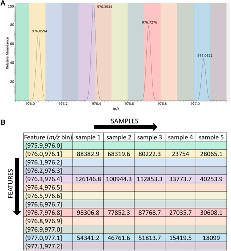
FIGURE 1. Visual depiction of the binning process. (A) 2 Da Range of spectrum from glycopeptide data set, with bin width set to 0.1 Da. Each colored slice of the spectrum represents a bin. (B) Data table depicting how data is arranged by LevR. The m/z value is the experimental m/z value from the spectrum. The feature is the narrow m/z range (bin) assigned to the experimental observation. Each sample occupies a column, and each sample-m/z pair contains the intensity of the m/z peak from the spectrum.
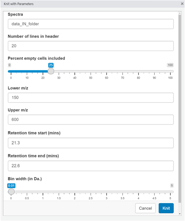
FIGURE 2. Graphical user interface (GUI) from LevR.
Figure 2 shows the interface the users see. The name of the folder with the data present is input, along with the mass range desired, the bin width, and the percent of empty bins allowable. After selecting the desired conditions, the software builds the data matrix of interest.
3.2 Test set one: Fingerprints
To test the utility of this approach for generating useful machine-learning ready data sets, we developed a challenge data set in-house by acquiring mass spectrometry data of fingerprints that had been subjected to two different storage conditions. While all the fingerprints were deposited onto aluminum foil, half the foil samples were immediately subjected to extraction with organic solvent. The other half of the samples were left to sit for 24 h prior to extraction. Previous researchers (Archer et al., 2005; Pleik et al., 2016; Pleik et al., 2018; Hinners et al., 2020) have indicated that some of the lipids in the fingerprints that are not immediately processed can undergo chemical changes, and this difference causes changes in a few peaks’ intensities in the mass spectrometry data. The fingerprint samples for the data set were acquired over numerous days and the MS data was acquired in two separate analyses more than a week apart. No effort was made to control other variables that may impact the lipid distribution, such as the depositor’s diet or exercise status or the laboratory conditions (e.g., heat, humidity, light). This was intentional so that the data would be sufficiently variable and challenging to classify. We sought to know whether it would be possible to classify the fingerprints’ age by simply extracting the full mass spectral data, binning it, as described above, and conducting supervised classification on the output matrix. If the classification were feasible in this paradigm, this outcome would demonstrate that the difficult up-front work of identifying the changing compounds may be eliminated. Furthermore, it would show that LevR could be applicable to a variety of other problems where researchers do not know whether a successful classification would be possible with their samples. This tool would enable screening of data for good classification outcomes prior to going through the laborious process of identifying the features that might be useful.
The data in Figure 3A clearly show that fingerprint age can be determined with a reasonable degree of accuracy using the data sets generated by LevR and classified by the Aristotle Classifier, a new classifier developed by our group. In Figure 3A, the output data from the Aristotle Classifier shows that a total of 70 samples are classified and about 85% are correctly assigned to their group. Using a leave-one-out cross-validation method, so test samples are never included in their training set, most of the (aged) samples, which are the first 35 samples shown, have Results of greater than zero, indicating that they are assigned to the aged group. By contrast, the non-aged samples, which range from Sample number 36 to 70 in the data set, mostly receive Results of less than zero, indicating that they are part of the non-aged group. A minority of the samples, which appear in red quadrants, were misclassified.

FIGURE 3. Comparison of Aristotle Classifier and PCA results for the fingerprint data set. (A) Results from the Aristotle Classifier for 70 fingerprint samples: 35 of each group (not aged and aged). Correctly classified samples are highlighted in the green quadrants. (B) PCA results of the same 70 fingerprint samples from panel (A)
The data in Figure 3B show a PCA plot of the same data used for supervised classification in Figure 3A. In this case, the two sets of samples, which are colored either orange or blue, are completely intermixed on the PCA plot. This Figure indicates that the difference imparted by leaving the samples out on a benchtop for a day was a small and difficult-to-detect difference, and other attributes contribute significantly more to the variability within the data. The samples would have separated into their respective groups (aged or not aged) had the difference in the samples due to the aging process been one of the most significant contributors to sample variability. Rather, the first two principal components represent more than 50% of the variability within the samples, and this variability is not attributable to the two different sample types.
In summary, the simple data processor, LevR, was useful for rapidly rendering a data matrix for 70 different lipidomics samples from deposited fingerprints. By coupling this software with a new machine learning tool, the Aristotle Classifier, the samples could be discriminated as either being aged or immediately processed, with reasonable accuracy (∼83%), even though the target differences in the sample were minor compared to other properties that contributed to the samples’ variability and features were not pre-selected for classification. This proof of concept, therefore, demonstrates the possibility of performing supervised machine learning directly on the full mass spectrometry data file for samples acquired by direct infusion experiments, without first identifying peaks of interest and quantifying them across a sample set.
3.3 Test set two: Glycopeptides
In a second analysis challenge, LC-MS data of glycopeptides from IgG were interrogated. In this case, the classification challenge was to determine whether the IgG glycoforms matched a native glycosylation profile or a non-native form, which was intentionally generated in the laboratory by modifying IgG with fucosidase, an enzyme that trims fucose off the IgG glycans. More details describing the samples and their preparation are in the Experimental section. In using LevR in a case like this, the retention time of interest needs to be determined a priori during a discovery experiment; the implementation of this tool assumes that the user has identified a chromatographic region of interest already and seeks to compare data in multiple samples at the given retention time.
The full mass spectral data including the elution window for the IgG glycoforms was used to build the data matrix, but only a small number of peaks within the data set carry the information content necessary to distinguish the two groups: Any bin that did not include peaks corresponding to glycopeptides would be uninformative. The data set contains 12,000 features (each corresponding to a 0.1 Da bin), in which only 120 features could be possibly associated with glycopeptides. (There were 15 identified glycopeptides, each populating up to eight bins with different isotopic peaks). Thus, the vast majority of the features would not be useful for classification. So, we again sought to determine whether extracting the MS data over the entire elution window for the glycopeptides, without including an identification step where the potentially relevant features were selected first, would lead to a viable data set that could be classified correctly.
The data in Figure 4 show the results of supervised (4a) and unsupervised (4b) classification of this data set. Figure 4A clearly shows that classification with the Aristotle Classifier was successful, and about 90% of the samples are correctly classified as either possessing a native or modified glycosylation profile. Likewise, the data in Figure 4B show that, as expected, the glycosylation difference is not the factor that generates most of the variability within the sample set. A plot of the first two principal components shows no ability to distinguish the native (blue) samples from the non-native (orange) ones. The fact that the samples were not readily separable by their principal components in Figure 4B is not surprising, because the change in glycosylation was subtle, and the vast majority of the features in the data set did not correspond to glycopeptide masses. Even considering the fact that the glycosylation difference is slight and that only a fraction of the peaks in the data set were impacted by this difference, the combined workflow of first extracting all of the MS data using LevR and then subjecting it to the Aristotle Classifier shows promise for machine learning applications on MS data, even in the case where the differences in the data set are subtle and lurking in a background of many uninformative peaks.

FIGURE 4. Comparison of Aristotle Classifier and PCA results for the full IgG glycopeptide data set. (A) Results from the Aristotle Classifier for 38 IgG glycopeptides: 19 of each group (native and partially defucosylated). Correctly classified samples are highlighted in the green quadrants. (B) PCA results of the same 38 IgG glycopeptide samples from panel (A)
The results in Figure 4A are exciting, but a logical next question is: could we have done better at classifying the data by limiting the analysis to only the glycopeptide peaks? Supervised learning methods, like the Aristotle Classifier, achieve their enhanced predictive power over unsupervised methods, like PCA, by weighting the features that best discriminate the two states more heavily than the uninformative features. (Although too many uninformative peaks can negatively impact the model’s performance.) We wanted to determine whether the classification would have been more successful had those uninformative features been removed in advance. Furthermore, we sought to verify that the glycopeptide peaks were, in fact, the ones that had been selected by the classifier as the “important features” in the classification shown in Figure 4A.
Determining which m/z regions in the spectra were weighted most heavily in the resulting classification is straightforward: The version of the Aristotle Classifier used for this work, AC.2021 (Hua and Desaire, 2021), includes a built-in matrix called FeatureCount which includes how each feature was weighted for the final result score for each sample. The feature counts can be positive, if the feature indicates the sample of interest is more like one sample type or negative, if the feature indicates that the sample is more like the alternative sample type. Therefore, to determine which features most impacted the classifier’s weightings overall, the absolute values of the feature counts were summed across the sample set. The resulting data is shown in Table 1 showing 19 of the top 20 features were associated with IgG glycoforms. For each of the IgG-related features, the relevant glycoform, FeatureCount, and bin are included. This result indicates that the embedded feature selection and weighting component of this particular classifier is effective at identifying the relevant features in the presence of many uninformative ones. (Note: because each feature is comprised of the ion counts from a small bin in the m/z space of the spectrum, each charge state of an ion, and indeed, each ion in every isotopic cluster, occupies its own bin and is therefore a unique feature.)

TABLE 1. Top 20 highest scoring features (m/z bins) as determined by the Aristotle Classifier. Within each glycoform section, features are ordered from highest to lowest scores, based on the sum of the absolute value of the FeatureCount. All features but one matched to an expected glycoform. Note, the m/z value includes the IgG2 peptide (EEQFNSTFR).
But could the classification be more successful if only the glycopeptides had been included in the first place? To answer this question, we first identified all the relevant m/z bins that would contain glycopeptide peaks, as described in the experimental section, and reclassified the data using only those features. The results appear in Figure 5A, for supervised classification, and Figure 5B, where the unsupervised PCA plot is provided. The PCA plot clearly shows that removing all the bins that do not contain glycopeptide information reduces the overall variability in the data, and the two sample types, natively glycosylated or modified, are now somewhat separable using this unsupervised method.
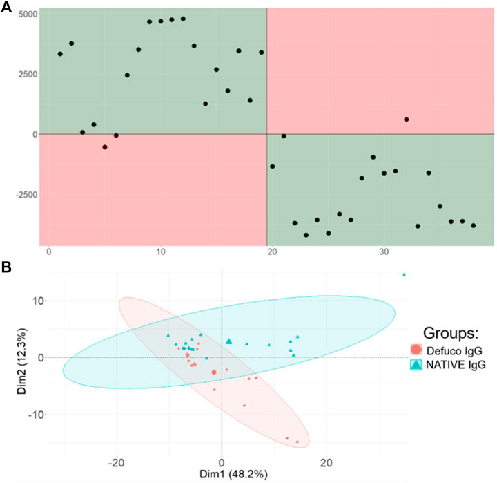
FIGURE 5. Comparison of Aristotle Classifier and PCA results for the refined IgG glycopeptide data set, including only features associated with glycopeptides. (A) Results from the Aristotle Classifier for 38 IgG glycopeptides data after removing all non-glycopeptide associated features. The misclassification rate did not change. The magnitude of the Y axis decreased slightly; this is due to a data set with reduced number of features. (B) PCA results for the refined IgG glycopeptide data set.
This outcome is consistent with the well-known principal that removing uninformative features generally improves one’s ability to discriminate the different biological states. Yet, the data in Figure 5A, showing the supervised classification of this data set with reduced features, is essentially identical to the result obtained in Figure 4A, where 12,000 uninformative features were still present in the data set. The fact that Figures 4A,5A look so similar is a desirable result: It unequivocally demonstrates that, when using the right kind of classifier, the data set need not be preprocessed to remove unnecessary, uninformative features. Rather, both the glycopeptide example and the fingerprint example in Figure 3, show that when a measurable difference is present in two different sample groups, machine learning and mass spectrometry can be exploited to identify that difference and classify samples into their respective groups, using the straight-forward workflow shown here.
4 Conclusion
The combined functionality of LevR and the Aristotle Classifier yields exciting results for mass spectrometrists and researchers studying biomarkers. LevR is a plain, yet effective, solution for formatting large amounts of mass spectrometry data. Its coupling to the Aristotle Classifier, a new machine learning tool, results in a powerful workflow that can be accessed by all researchers regardless of coding experience. This workflow and tool will be useful for biomarker discovery, in which biological samples can be analyzed by mass spectrometry, the data can be formatted automatically, and the classifier can render results to indicate if there are detectable differences between the healthy and disease state of the biological samples. Further, the classifier’s results can be leveraged to identify which features contribute most to the difference between sample types.
Data availability statement
The raw data supporting the conclusions of this article will be made available by the authors, without undue reservation.
Author contributions
Did experiments: LP, MP. Wrote manuscript: LP, MP, and HD.
Conflict of interest
The authors declare that the research was conducted in the absence of any commercial or financial relationships that could be construed as a potential conflict of interest.
Publisher’s note
All claims expressed in this article are solely those of the authors and do not necessarily represent those of their affiliated organizations, or those of the publisher, the editors and the reviewers. Any product that may be evaluated in this article, or claim that may be made by its manufacturer, is not guaranteed or endorsed by the publisher.
Supplementary Material
The Supplementary Material for this article can be found online at: https://www.frontiersin.org/articles/10.3389/frans.2022.961592/full#supplementary-material
References
Acharjee, A., Prentice, P., Acerini, C., Smith, J., Hughes, I. A., Ong, K., et al. (2017). The translation of lipid profiles to nutritional biomarkers in the study of infant metabolism. Metabolomics 13 (3), 25. doi:10.1007/s11306-017-1166-2
Archer, N. E., Charles, Y., Elliott, J. A., and Jickells, S. (2005). Changes in the lipid composition of latent fingerprint residue with time after deposition on a surface. Forensic Sci. Int. 154 (2), 224–239. doi:10.1016/j.forsciint.2004.09.120
Atherton, T., Croxton, R., Baron, M., Gonzalez-Rodriguez, J., Gamiz-Gracia, L., and Garcia-Campana, A. M. (2012). Analysis of amino acids in latent fingerprint residue by capillary electrophoresis-mass spectrometry. J. Sep. Sci. 35 (21), 2994–2999. doi:10.1002/jssc.201200398
Barthélemy, M., Guérineau, V., Genta-Jouve, G., Roy, M., Chave, J., Guillot, R., et al. (2020). Identification and dereplication of endophytic Colletotrichum strains by MALDI TOF mass spectrometry and molecular networking. Sci. Rep. 10 (1), 19788. doi:10.1038/s41598-020-74852-w
Bouslimani, A., Melnik, A. V., Xu, Z., Amir, A., da Silva, R. R., Wang, M., et al. (2016). Lifestyle chemistries from phones for individual profiling. Proc. Natl. Acad. Sci. U. S. A. 113 (48), E7645–E7654. doi:10.1073/pnas.1610019113
Desaire, H., and Hua, D. (2020). Adaption of the Aristotle classifier for accurately identifying highly similar bacteria analyzed by MALDI-TOF MS. Anal. Chem. 92 (1), 1050–1057. doi:10.1021/acs.analchem.9b04049
Desaire, H., Patabandige, M. W., and Hua, D. (2021). The local-balanced model for improved machine learning outcomes on mass spectrometry data sets and other instrumental data. Anal. Bioanal. Chem. 413 (6), 1583–1593. doi:10.1007/s00216-020-03117-2
Ferguson, L. S., Wulfert, F., Wolstenholme, R., Fonville, J. M., Clench, M. R., Carolan, V. A., et al. (2012). Direct detection of peptides and small proteins in fingermarks and determination of sex by MALDI mass spectrometry profiling. Analyst 137 (20), 4686–4692. doi:10.1039/c2an36074h
He, L., Diedrich, J., Chu, Y. Y., and Yates, J. R. (2015). Extracting accurate precursor information for tandem mass spectra by RawConverter. Anal. Chem. 87 (22), 11361–11367. doi:10.1021/acs.analchem.5b02721
Hinners, P., O’Neill, K. C., and Lee, Y. J. (2018). Revealing individual lifestyles through mass spectrometry imaging of chemical compounds in fingerprints. Sci. Rep. 8 (1), 5149. doi:10.1038/s41598-018-23544-7
Hinners, P., Thomas, M., and Lee, Y. J. (2020). Determining fingerprint age with mass spectrometry imaging via ozonolysis of triacylglycerols. Anal. Chem. 92 (4), 3125–3132. doi:10.1021/acs.analchem.9b04765
Hua, D., and Desaire, H. (2021). Improved discrimination of disease states using proteomics data with the updated Aristotle classifier. J. Proteome Res. 20 (5), 2823–2829. doi:10.1021/acs.jproteome.1c00066
Hua, D., Liu, X., Go, E. P., Wang, Y., Hummon, A. B., and Desaire, H. (2020). How to apply supervised machine learning tools to MS imaging files: Case study with cancer spheroids undergoing treatment with the monoclonal antibody cetuximab. J. Am. Soc. Mass Spectrom. 31 (7), 1350–1357. doi:10.1021/jasms.0c00010
Hua, D., Patabandige, M. W., Go, E. P., and Desaire, H. (2019). The Aristotle classifier: Using the whole glycomic profile to indicate a disease state. Anal. Chem. 91 (17), 11070–11077. doi:10.1021/acs.analchem.9b01606
Huang, Y.-C., Chung, H.-H., Dutkiewicz, E. P., Chen, C.-L., Hsieh, H.-Y., Chen, B.-R., et al. (2020). Predicting breast cancer by paper spray ion mobility spectrometry mass spectrometry and machine learning. Anal. Chem. 92 (2), 1653–1657. doi:10.1021/acs.analchem.9b03966
Hyde, J., and Runyon, J. R. (2020). LCMS measurement of steroid biomarkers collected from palmar sweat. ChemRxiv. doi:10.26434/chemrxiv.12931769
Ifa, D. R., Manicke, N. E., Dill, A. L., and Cooks, R. G. (2008). Latent fingerprint chemical imaging by mass spectrometry. Sci. Wash. D.C. U. S.) 321 (5890), 805. doi:10.1126/science.1157199
Ishii, H., Sakamoto, K., Ashizawa, K., Masuyama, K., Saitoh, M., Sakamoto, K., et al. (2020). Lipidome-based rapid diagnosis with machine learning for detection of TGF-β signalling activated area in head and neck cancer. Br. J. Cancer 122 (7), 995–1004. doi:10.1038/s41416-020-0732-y
Kassambara, A., and Mundt, F. (2020). factoextra: Extract and visualize the results of multivariate data analyses, Vetsion: 1.0.7
Liebal, U. W., Phan, A. N. T., Sudhakar, M., Raman, K., and Blank, L. M. (2020). Machine learning applications for mass spectrometry-based metabolomics. Metabolites 10 (6), 243. doi:10.3390/metabo10060243
Manzi, M., Palazzo, M. n., Knott, M. a. E., Beauseroy, P., Yankilevich, P., Giménez, M. a. I., et al. (2021). Coupled mass-spectrometry-based lipidomics machine learning approach for early detection of clear cell renal cell carcinoma. J. Proteome Res. 20 (1), 841–857. doi:10.1021/acs.jproteome.0c00663
Mészáros, B., Járvás, G., Kun, R., Szabó, M., Csánky, E., Abonyi, J., et al. (2020). Machine learning based analysis of human serum N-glycome alterations to follow up lung tumor surgery. Cancers 12 (12), E3700. doi:10.3390/cancers12123700
Mirabelli, M. F., Chramow, A., Cabral, E. C., and Ifa, D. R. (2013). Analysis of sexual assault evidence by desorption electrospray ionization mass spectrometry. J. Mass Spectrom. 48 (7), 774–778. doi:10.1002/jms.3205
O'Neill, K. C., Hinners, P., and Lee, Y. J. (2020). Potential of triacylglycerol profiles in latent fingerprints to reveal individual diet, exercise, or health information for forensic evidence. Anal. Methods 12 (6), 792–798. doi:10.1039/c9ay02652e
O'Neill, K. C., and Lee, Y. J. (2018). Effect of aging and surface interactions on the diffusion of endogenous compounds in latent fingerprints studied by mass spectrometry imaging. J. Forensic Sci. 63 (3), 708–713. doi:10.1111/1556-4029.13591
Pleik, S., Spengler, B., Ram Bhandari, D., Luhn, S., Schäfer, T., Urbach, D., et al. (2018). Ambient-air ozonolysis of triglycerides in aged fingerprint residues. Analyst 143 (5), 1197–1209. doi:10.1039/c7an01506b
Pleik, S., Spengler, B., Schäfer, T., Urbach, D., Luhn, S., and Kirsch, D. (2016). Fatty acid structure and degradation analysis in fingerprint residues. J. Am. Soc. Mass Spectrom. 27 (9), 1565–1574. doi:10.1007/s13361-016-1429-6
R Core Team, R. (2020). A language and environment for statistical computing. Vienna, Austria: R Foundation for Statistical Computing.
Shetage, S. S., Traynor, M. J., Brown, M. B., and Chilcott, R. P. (2018). Sebomic identification of sex- and ethnicity-specific variations in residual skin surface components (RSSC) for bio-monitoring or forensic applications. Lipids Health Dis. 17 (1), 194. doi:10.1186/s12944-018-0844-z
Sho, K., Kentaro, Y., Junichi, A., Takashi, K., Hiroyuki, H., Meguri, T., et al. (2021). A new rapid diagnostic system with ambient mass spectrometry and machine learning for colorectal liver metastasis. BMC cancer 21 (1), 1–9. doi:10.1186/s12885-021-08001-5
Smith, C. A., Want, E. J., O'Maille, G., Abagyan, R., and Siuzdak, G. (2006). Xcms: Processing mass spectrometry data for metabolite profiling using nonlinear peak alignment, matching, and identification. Anal. Chem. 78 (3), 779–787. doi:10.1021/ac051437y
Stanstrup, J., Broeckling, C. D., Helmus, R., Hoffmann, N., Mathé, E., Naake, T., et al. (2019). The metaRbolomics toolbox in bioconductor and beyond. Metabolites 9 (10), E200. doi:10.3390/metabo9100200
Tang, H.-W., Lu, W., Che, C.-M., and Ng, K.-M. (2010). Gold nanoparticles and imaging mass spectrometry: Double imaging of latent fingerprints. Anal. Chem. Wash. D.C. U. S.) 82 (5), 1589–1593. doi:10.1021/ac9026077
Tang, X., Huang, L., Zhang, W., and Zhong, H. (2015). Chemical imaging of latent fingerprints by mass spectrometry based on laser activated electron tunneling. Anal. Chem. Wash. D.C. U. S.) 87 (5), 2693–2701. doi:10.1021/ac504693v
van Helmond, W., van Herwijnen, A. W., van Riemsdijk, J. J. H., van Bochove, M. A., de Poot, C. J., and de Puit, M. (2019). Chemical profiling of fingerprints using mass spectrometry. Forensic Chem. 16, 100183. doi:10.1016/j.forc.2019.100183
van Oosten, L. N., and Klein, C. D. (2020). Machine learning in mass spectrometry: A MALDI-TOF ms approach to phenotypic antibacterial screening. J. Med. Chem. 63 (16), 8849–8856. doi:10.1021/acs.jmedchem.0c00040
Weis, C. V., Jutzeler, C. R., and Borgwardt, K. (2020). Machine learning for microbial identification and antimicrobial susceptibility testing on MALDI-TOF mass spectra: A systematic review. Clin. Microbiol. Infect. 26 (10), 1310–1317. doi:10.1016/j.cmi.2020.03.014
Wickham, H., Averick, M., Bryan, J., Chang, W., McGowan, L., Francois, R., et al. (2019). Welcome to the tidyverse. J. Open Source Softw. 4 (43), 1686. doi:10.21105/joss.01686
Wickham, H., Francois, R., Henry, L., and Muller, K. (2021). Data from: A Gramm. Data Manip. dplyr5. 1.0.
Xie, Y. R., Castro, D. C., Bell, S. E., Rubakhin, S. S., and Sweedler, J. V. (2020). Single-cell classification using mass spectrometry through interpretable machine learning. Anal. Chem. 92 (13), 9338–9347. doi:10.1021/acs.analchem.0c01660
Yagnik, G. B., Korte, A. R., and Lee, Y. J. (2013). Multiplex mass spectrometry imaging for latent fingerprints. J. Mass Spectrom. 48 (1), 100–104. doi:10.1002/jms.3134
Zhang, J., Du, Q., Song, X., Gao, S., Pang, X., Li, Y., et al. (2020). Evaluation of the tumor-targeting efficiency and intratumor heterogeneity of anticancer drugs using quantitative mass spectrometry imaging. Theranostics 10 (6), 2621–2630. doi:10.7150/thno.41763
Zhang, L., Ma, F., Qi, A., Liu, L., Zhang, J., Xu, S., et al. (2020). Integration of ultra-high-pressure liquid chromatographytandem mass spectrometry with machine learning for identifying fatty acid metabolite biomarkers of ischemic stroke. Chem. Commun. 56 (49), 6656–6659. doi:10.1039/d0cc02329a
Keywords: mass spectrometry, machine learning, fingerprint, analytical methods, lipidomics, glycopeptide analysis, IgG glycosylation
Citation: Pfeifer LD, Patabandige MW and Desaire H (2022) Leveraging R (LevR) for fast processing of mass spectrometry data and machine learning: Applications analyzing fingerprints and glycopeptides. Front. Anal. Sci. 2:961592. doi: 10.3389/frans.2022.961592
Received: 04 June 2022; Accepted: 20 July 2022;
Published: 23 August 2022.
Edited by:
Emmanuelle Lipka, Faculty of Pharmacy, Lille University, FranceReviewed by:
Geer Teng, Beijing Institute of Technology, ChinaNoortje De Haan, University of Copenhagen, Denmark
Copyright © 2022 Pfeifer, Patabandige and Desaire. This is an open-access article distributed under the terms of the Creative Commons Attribution License (CC BY). The use, distribution or reproduction in other forums is permitted, provided the original author(s) and the copyright owner(s) are credited and that the original publication in this journal is cited, in accordance with accepted academic practice. No use, distribution or reproduction is permitted which does not comply with these terms.
*Correspondence: Heather Desaire, aGRlc2FpcmVAa3UuZWR1