Use of Hyper-Spectral Visible and Near-Infrared Satellite Data for Timely Estimates of the Earth’s Surface Reflectance in Cloudy and Aerosol Loaded Conditions: Part 1–Application to RGB Image Restoration Over Land With GOME-2

1 Introduction

Surface properties derived from satellite solar backscattered ultraviolet (UV) through near- and short-wave infrared (NIR, SWIR) reflectances have a multitude of uses for studies on marine and terrestrial biogeochemistry, including the response of ecosystems to climate variability, change, and feedback processes as well as time-sensitive applications such as drought or other hazard detection (e.g., Anyamba and Tucker, 2012; Yuan et al., 2014; AghaKouchak et al., 2015; Frouin et al., 2019; Groom et al., 2019). A cornerstone of many satellite-based scientific studies involving the Earth’s surface is atmospheric correction, the process of removing the effects of the atmosphere and other factors, when processing satellite radiance data. The corrections need to account for the effects of absorbing and scattering gases and particles in the Earth’s atmosphere. Additional corrections may be needed in order to remove unwanted surface signals such as from ocean glitter or shadows. Atmospheric correction remains an active area of research for Earth remote sensing (e.g., Frouin et al., 2019).

Satellite instruments in Low or Geostationary Earth Orbits (LEO, GEO), including multi-angle and polarization-sensitive sensors, have provided surface reflectances and albedos at wavelength bands from UV to the SWIR (Duchemin and Maisongrande, 2002; Govaerts et al., 2004; Maignan et al., 2004; Diner et al., 2005; Muller et al., 2007; Claverie et al., 2018; He et al., 2019; Li S. et al., 2019). In this work, we use data from the MODerate-resolution Imaging Spectroradiometer (MODIS) instruments in LEO. There are several available MODIS land surface reflectance data sets, including some that have undergone detailed processing in the time domain to quantify bidirectional reflectance distribution functions (BRDFs) that describe how the surface reflectance varies with the sun-satellite geometry. These include the nadir BRDF-adjusted reflectance (NBAR), also known as the MODIS MCD43 product (Schaaf et al., 2002; Wang et al., 2018), and the Multi-Angle Implementation of Atmospheric Correction (MAIAC), known as the MCD19 product (Lyapustin et al., 2011a; Lyapustin et al., 2011b; Lyapustin et al., 2012). Deriving the terrestrial BRDF and optional information regarding aerosol properties necessitates complex algorithms that use data acquired over a window of time with assumptions regarding variability over the considered time period. As a result of the processing required over the time window (typically 16 days), data sets may not be immediately available after the satellite overpass. In addition, these algorithms also detect and remove pixels that are affected by clouds; this can significantly reduce the available spatial coverage (e.g., Banks and Mélin, 2015). For example, Mercury et al. (2012) showed that globally a cloud cover of around 28% is found with MODIS data at 5 km × 5 km resolution.

In this work, we examine whether it is possible to reconstruct red, green, and blue (RGB) land surface reflectances in cloudy conditions using nearly all-sky satellite-based radiances measured by hyper-spectral instruments. The satellite instrument that we use is the Global Ozone Monitoring Experiment 2 (GOME-2) that was designed primarily for atmospheric composition measurements. GOME-2 offers continuous spectral coverage from the UV through NIR (240–790 nm). Specifically in this work, we test whether the spectral measurements in the visible through NIR (403–790 nm) from GOME-2 can be used to accurately estimate the underlying land surface reflectances in cloudy pixels with machine learning trained on NBARs from the MODIS MCD43 data set that was found to perform well for estimating the gross primary production of vegetation (Joiner et al., 2018). In addition, we test the approach using discrete wavelength windows to determine the most important ranges for reconstruction of RGB surface reflectances in cases of light to moderate amounts of cloud and heavy aerosol loading.

The basic assumption behind our approach is that a machine learning method, such as an artificial neural network (NN), is capable of disentangling and extracting a surface spectral fingerprint (in this case, as it relates to RGB land reflectances) from observed spectral reflectances. These observations are affected by scattering and absorption from air molecules (Rayleigh and Raman scattering and absorption from gases such as O₂, H₂O, NO₂, and O₃), aerosols, and clouds. The use of deep learning with NNs as well as other types of machine learning has seen explosive growth in many areas of remote sensing including hyperspectral image analysis such as for tasks in image classification, anomaly detection, target recognition, parameter inversion, pansharpening, and data fusion from preprocessing to mapping (see, e.g., the reviews of Lary et al., 2016; Zhu et al., 2017; Maxwell et al., 2018; Ma et al., 2019, and references therein).

Here, a principal component analysis is used to precondition the spectral inputs to the NNs. Similar methods have been employed in ocean remote sensing in the presence of aerosol, thin clouds, and Sun glint using simulated data for training (e.g., Gross-Colzy et al., 2007a, Gross-Colzy et al., 2007b; Schroeder et al., 2007). Our approach uses a large sample of measured spectra from a satellite instrument rather than simulated data for training inputs. The resulting trained NN is then applied globally for 1 year for evaluation under a wide range of conditions. In addition, we test the approach for observations with optically thicker clouds than previously attempted (clouds that appear white to the human eye) as well as cases of heavy absorbing aerosol loading. We show with radiative transfer simulations that there is sensitivity to the Earth’s surface as seen from satellite-based instruments even in cases of cloud optical thickness exceeding ten. In a companion work, Joiner et al. (2021) employ a similar approach with a higher spatial resolution hyper-spectral imager and examine remote sensing of vegetation using near-infrared bands in a case study that contains overcast cloud conditions.

Our approach is fundamentally different from other image restoration methods that rely on either the availability of temporally adjacent clear sky reference images (temporal methods), estimates of the surface reflectance (spatial methods), or remaining parts of an image (non-complementation methods) (e.g., Zhang et al., 2018; Wang et al., 2019; Li et al., 2019b, and references therein). Spectral methods have been employed in image dehazing that has far ranging applications in Earth science, search and rescue, event recognition, and aerial surveillance (e.g., Mehta et al., 2021, and references therein). Spectral approaches have also been employed for ocean remote sensing (e.g., Steinmetz et al., 2011; Frouin et al., 2014; Frouin and Gross-Colzy, 2016). Here, we describe a spectral method that encompasses and goes beyond dehazing and can be described as spectral cloud clearing. Beyond the RGB information provided in the training data set, our approach does not require any additional a priori information about the Earth’s surface or atmospheric absorption or scattering, nor does it require radiative transfer calculations or look up tables. The ultimate success of the method does however require a high quality sample of training data.

2 Materials and Methods

2.1 GOME-2 Spectra

We use reflectance measurements from GOME-2 (Munro et al., 2016), a satellite instrument with spectral coverage from the UV to the NIR including the so-called red edge from approximately 670 nm through the start of the strong O₂ A band near 758 nm. This instrument has a spectral resolution of the order of 0.5 nm at the wavelengths of interest (∼400–800 nm). It flies on the European Meteorological Satellites operational (EUMETSAT MetOp) series. Here, we use data from GOME-2A (aboard MetOp-A) in 2018. MetOp-A, launched on October 19, 2006, is in a LEO with a local equator crossing time near 09:30. We use data from GOME-2 bands 3 and 4 covering 397–604 and 593–790 nm, respectively. We used GOME-2A level 1B data from version R2 with no further adjustments. In 2018, GOME-2 was collecting data in a reduced swath mode (960 km swath), with pixels sizes approximately 40 × 40 km² at nadir. While this spatial resolution is considered low for many applications, the algorithm developed here and tested with GOME-2 can be implemented and evaluated with higher spatial resolution hyper-spectral imagers.

2.2 MODIS MCD43 and Other Land Data Sets

We use NBAR data from the collection 6 MODIS MCD43C data set (Schaaf et al., 2002; Schaaf, 2015; Wang et al., 2018). MODIS instruments fly on the National Aeronautics and Space Administration (NASA) Terra and Aqua satellites in late morning (10:30 equator crossing time) and early afternoon (13:30 equator crossing time) polar orbits, respectively. Among the available MODIS bands, here, we use bands 1, 4, and 3, corresponding to red (R, 620–670 nm), green (G, 545–565 nm), and blue (B, 459–479 nm), respectively, that fall within the GOME-2 spectral range. MCD43 NBARs are reported on a daily basis. These data are constructed from clear-sky reflectance data observed over a 16 days window, computed on a daily basis and weighted towards the reported day. Therefore, these data are not true daily data, but rather can be considered as somewhat smoothed over a rolling 16 days window. The MCD43C NBAR data are averaged on a grid of 0.05° latitude by 0.05° longitude.

We collocate MCD43C data to GOME-2 footprints by averaging all NBARs for gridboxes whose centers fall within the rectangular area defined by the corners of a given GOME-2 pixel. We similarly compute the fraction of snow in a GOME-2 pixel according to the Interactive Multi-sensor Snow and ice mapping system (IMS) data set (U.S. National Ice Center, 2008) in the northern hemisphere and the Near-real-time Ice and Snow Extent (NISE) data set (Brodzik and Stewart, 2016) in the southern hemisphere. We also calculate the fraction of water-cover within a GOME-2 pixel as in Qin et al. (2019).

2.3 Neural Network Architecture

Figure 1 describes the general approach of training a neural network (NN) to estimate RGB land surface reflectances (henceforth denoted RGB_G2 or R_G2, G_G2, B_G2) from all-sky GOME-2 spectra.

FIGURE 1

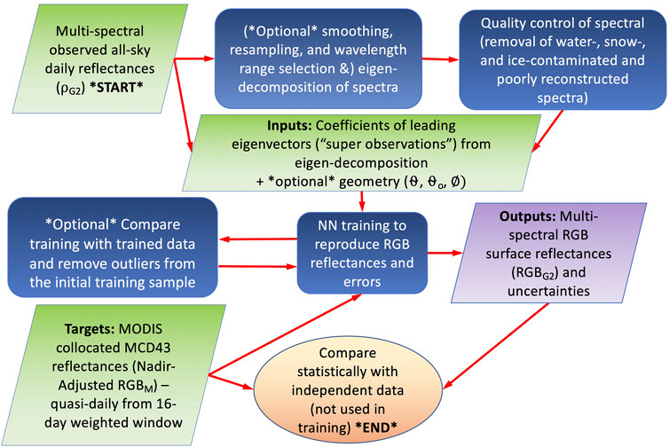
FIGURE 1. Flow diagram showing how RGB surface reflectances and their uncertainties are estimated with machine learning (a neural network, NN) using continuous hyper-spectral measurements from instruments such as GOME-2 trained on MODIS RGB (RGB_M) surface reflectances.

In order to reduce the dimensions of the GOME-2 spectral measurements used as predictors (shown in the top left box in Figure 1), we perform an principal component analysis (or eigen-decomposition) of the input spectra, in the form of a covariance matrix. To train the NN, we use GOME-2 data from all orbits on several days encompassing all seasons (Jan. 2-3, Mar. 2-3, May 2-3, Jul. 6-7, Sep. 3-4, and Nov. 2-3 of 2018). The dates were chosen to avoid days when GOME-2A was operating in a more narrow swath mode. The 2 days in each chosen month were selected to provide good coverage over all land masses. While we have not undertaken a detailed study on the sampling of data needed for good global results, we find that this sample appears to be adequate as will be shown below.

The eigen-decomposition is accomplished using all spectra from these days. We then compute coefficients of the leading eigen-modes in order to represent each spectrum with these leading modes. The number of included leading modes was optimized as discussed below. The leading mode coefficients can then be thought of as pseudo-observations to be used as predictors or features in the NN training rather than the full spectral complement. Before the eigen-decomposition, there are additional options to select a particular wavelength range, spectral resolution (by smoothing the GOME-2 spectra), and spectral sampling. These options can be used to simulate performance for other instruments.

The next step in the process is quality assurance, which we found to be critical to the overall performance of the NN. The quality assurance tests, developed by trial and error, were found to give good performance of the trained NN as compared with independent data as described below. We use the following quality assurance (QA) checks in order to flag potentially erroneous training and evaluation data over land only. They include the removal of spectra over 1) snow and ice; 2) water; 3) optically thick clouds; 4) scenes with high Solar Zenith Angles (SZAs $>\mathrm{70}°$); and 5) spectra that cannot be well reconstructed with the leading modes.

We obtained superior training results when data over snow were removed from the training sample. The spectral signature of the snow for the wavelengths used here may be confused with that of clouds. In addition, the MCD43 algorithm may not produce appropriate daily NBARs for training in the presence of partial or rapidly changing snow conditions. We remove all pixels with snow or ice fraction $>$ 5% as determined by the IMS and NISE data. We found a few remaining snow contaminated pixels, particularly in the southern hemisphere where the IMS data were not available. To remove these, we filter data using the empirically derived expression G_M - (1.5 B_M - 0.02) $<$ 0.

We also found that eliminating mixed land/water pixels improved performance as water reflectance properties may not be well-captured within MCD43. We eliminate all pixels with water fractions $>$ 5%. To remove optically thick clouds, we filter out all pixels with a red reflectance, ρ_G2, $>$ 0.6.

We then eliminate spectra by evaluating the reconstruction with leading modes as follows. For each spectrum, the error in the spectrum reconstructed with the leading modes (defined as the difference between the reconstructed spectrum and the original spectrum) is computed for every wavelength. If the maximum absolute error for a given spectrum is 5 times more than the standard deviation of reconstruction errors computed over all the wavelengths of all spectra in the training set, then that spectrum is excluded from the training and evaluation samples; this flagging may identify damaged spectra, such as those with large noise found in the south Atlantic Anomaly area and those potentially affected by saturation in glint conditions as discussed by Gorkavyi et al. (2021).

The collocated MODIS MCD43-based RGB NBARs (denoted RGB_M or R_M, G_M, B_M) are used as the predicted or target variables. These MODIS data are derived from observations made in clear skies over a rolling 16 days period. They may be considered as clear sky data adjusted to remove atmospheric, aerosol, and sun-satellite geometric effects, interpolated to the location of cloud, aerosol, and atmospheric-contaminated GOME-2 data. The coefficients of the leading eigenvectors of GOME-2 spectra that have passed all quality assurance checks are the predictors. Optionally, sun-satellite geometry parameters can be added as predictors. Here, we use the cosines of the SZA, view zenith angles, and phase angles, θ₀, θ, and ϕ, respectively, where the phase angle is defined as the angle at a given point between the Sun and satellite. The resulting NN training can be described by

${\mathrm{R}\mathrm{G}\mathrm{B}}_{\text{G}2}=f_{\text{NN}}\left({\rho }_{G2},\cos \left({\theta }_0\right),\cos \left(\theta \right),\cos \left(\varphi \right)\right).(1)$

The NN basically acts as a non-linear regression function that attempts to separate the spectral signature of the surface reflectance from that of the atmosphere including clouds, aerosol, and gaseous absorption. We provide more interpretation of how the NN is able to perform this separation below.

The NN training is performed with half of the available samples from the above-mentioned dates that pass all quality assurance tests. After the training process has converged, results generated from the trained NN are applied to independent GOME-2 predictor data and are then compared with collocated MODIS data for samples not used in the training. An optional step at this point is to check for outliers and fine tune the quality control to remove these data. This is how we developed the final quality assurance checks. The trained NN can then be used to apply the cloud clearing globally in a simple and efficient manner, requiring only the eigenvectors and weights of the NN.

The reconstruction errors for the three color bands, denoted RGB_error, can be similarly estimated by training a second NN with the same predictors but with targets consisting of absolute values of the differences between GOME-2 reconstructed and corresponding collocated MODIS reflectances, i.e.,

$\mathrm{R}\mathrm{G}\mathrm{B}\text{\_}\mathrm{e}\mathrm{r}\mathrm{r}\mathrm{o}\mathrm{r}=f_{\text{NN}}\left({\rho }_{G2},\cos \left({\theta }_0\right),\cos \left(\theta \right),\cos \left(\varphi \right)\right).(2)$

The reconstruction error standard deviation is then given by RGB_error × 1.25 assuming a normal distribution.

We employ the same general NN architecture as that used by Joiner and Yoshida (2020) for estimation of gross primary production (GPP) from MODIS NBARs. Briefly, a configuration within the Interactive Data Language (IDL) software package consists of a three layer feed-forward artificial NN with two hidden layers and 2N nodes in each layer, where N is the number of inputs. The output layer has three nodes, one each for R, G, and B NBAR; this produced similar results as when separate networks were created for each of the output bands. For activation functions we use a soft-sign for the first layer, a logistic (sigmoid) for the second layer, and a bent identity for the third layer. An adaptive moment estimation optimizer minimizes the error function with a learning rate of 0.1. Inputs and outputs are both scaled to produce zero means and unit standard deviations. Similar results were reproduced with Python codes and different architectures.

While we have eliminated both snow and water contaminated pixels here, we note that this does not mean that our approach is not applicable to either snow- or water-covered pixels. For example, the use of short-wave infrared bands (not available on GOME-2) along with an appropriate training data set over snow may enable the approach to be applied over snow-covered surfaces. Similarly, applications over water surfaces should also be possible with appropriate training data.

3 Results

Figure 2 shows a random sample of GOME-2 spectra under various conditions ranging from mostly clear (those with lowest reflectances) to highly cloudy (those with the highest reflectances). Several gaseous absorption bands are seen including the O₂ B band near 685 nm and the O₂ A band near ∼760 nm. The rapid rise in reflectance between about 685 and 760 nm, known as the red edge, is apparent particularly in the mostly clear sky pixels. In general, clouds tend to flatten out the spectra. The effect of increased Rayleigh scattering at shorter (bluer) wavelengths is also apparent in the all sky reflectances; this is manifested as increasing reflectances from green to blue wavelengths although the surface reflectance is generally lower in the blue as compared with the green.

FIGURE 2

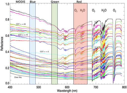
FIGURE 2. Random sampling of GOME-2 spectra (colors chosen at random) on various days in 2018 with major atmospheric gaseous absorption bands labeled above and MODIS bands indicated as labeled above and approximate values of cloud optical thicknesses (COT) (assuming overcast conditions) and conditions (e.g., Clear Sky) labeled near the corresponding spectra.

3.1 Dependence on Inputs

We perform a series of NN trainings and evaluations using different wavelength ranges along with optional smoothing and resampling of the spectra to simulate other instruments. With the full spectral range, resolution, and sampling of GOME-2, we can simulate and compare the potential performance of various current and future satellite instruments. Table 1 summarizes the evaluations with statistics comparing reconstructed RGB_G2 with the target RGB_M.

TABLE 1

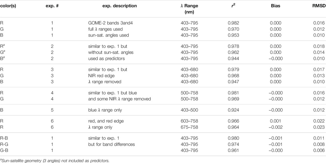
TABLE 1. Statistical comparison of 131,544 GOME-2 independent (not used in training) data points with collocated MODIS data from training/evaluation days listed above. Statistics include the root mean squared difference (RMSD), bias (mean of RGB_G2–RGB_M), and variance explained (r²). The table is segmented into different experiments, denoted by “exp. #”. The last grouping is for band differences.

We find that 14 coefficients of the leading eigenvectors is close to optimal for RGB estimation using the full wavelength range of 403–795 nm. There is no apparent benefit from using additional eigenvectors (results not shown) and some degradation with less than 14. The leading eigenvectors (principal components) are shown in Supplementary Figures S1, S2. Correlations and root mean squared difference (RMSD) are highest for the red band and lowest for blue which may reflect differences in the signal to noise ratios in the different bands.

The reconstruction of NBARs includes not only atmospheric correction and cloud and/or aerosol clearing, but also the BRDF adjustment to nadir viewing. This use of the three angles that define the sun-satellite geometry as predictors helps in this respect. We conducted another training without using these angles as predictors. The results of exp. #2 in Table 1 without angles as predictors show a relatively small degradation as compared with results that used the sun-satellite angles in exp. #1. This is an indication that the NN is learning about the canopy scattering and shadowing directly from the spectra. The NN also appears to learn how to deal with complex cloud and aerosol bi-directional effects from the spectra.

Nearly identical results are obtained using the full wavelength range of GOME-2 bands 3 and 4 and a reduced range that removes wavelengths in the O₂ A band (403–758 nm) (not shown). A small degradation is seen with the reduced wavelength range of 403–680 nm where red edge wavelengths are removed (exp. #3 of Table 1). Removing wavelengths in the blue region (using 500–758 nm in exp. #4) does not produce substantial degradation for the red and green bands. Using only wavelengths in the blue range (403–500 nm) produces noticeable degradation to the reconstruction of blue reflectance (exp. #5), although the overall RMSD may be acceptable for some applications. This wavelength range would be applicable to the Ozone Monitoring Instrument (OMI) that is used to estimate column amounts of trace gases such as NO₂ and does not cover green or red wavelengths. Using red through the red edge (603–758 nm, exp. #6) produces some degradation in statistics for the red band as compared to results obtained with the green through red wavelength range.

We simulate RGB reconstruction that would be achieved using a lower spectral resolution hyper-spectral sensor such as the planned NASA Plankton, Aerosol, Cloud, ocean Ecosystem (PACE) Ocean Color Instrument (OCI) that will have spectral coverage from the UV through the NIR at approximately 5 nm spectral resolution and at 1 km spatial resolution (Werdell et al., 2019). We averaged together every 25 GOME-2 samples (GOME-2 sampling is approximately 0.21 nm) to produce PACE-like spectra. We obtain negligible degradation in RGB estimates as compared with those obtained using full GOME-2 spectral resolution with the same wavelength range (not shown). Further testing by averaging every 50 GOME-2 samples produced similar results (not shown), indicating that high spectral resolution is not required in order to achieve good surface reflectance estimates in cloudy conditions.

We computed the full error covariance of the GOME-2 surface RGB reconstruction. We find that the errors for all bands are substantially correlated. This bodes well for applications that rely upon ratios or differences of bands, such as in the computation of some vegetation indices. The error correlation between red and blue is 0.73, red and green is 0.85, and green and blue is 0.89. We list statistics for band differences in Table 1 (last grouping, for exp. #1) that shows, as expected based on the error correlations, higher correlations between target and predicted surfaces reflectances for band differences as compared with some of the individual bands.

3.2 Dependence on Cloudiness

Figure 3A shows two dimensional (2D) density plots comparing the target R_M with the reconstructed R_G2 using the range 400–795 nm on August 2, 2018, a day not used in the NN training. The r² value is 0.97, and the overall bias is negligible. However, a small bias is shown at lower values of R_M.

FIGURE 3

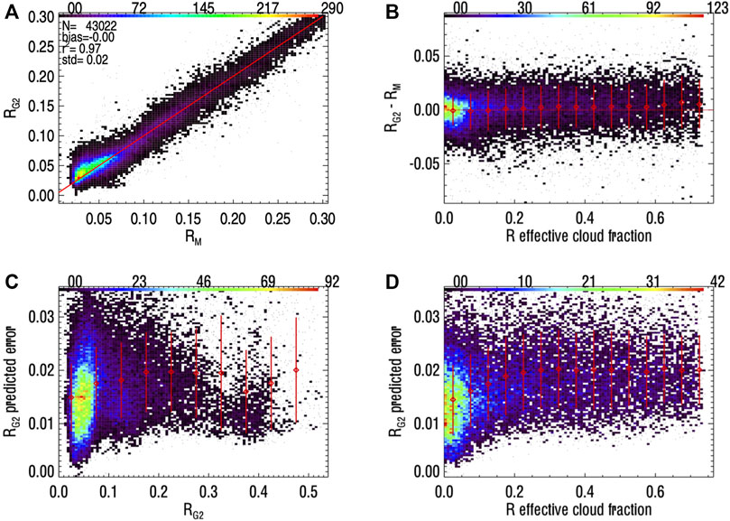
FIGURE 3. Density plots using (independent) red band data (denoted “R”) from August 2, 2018 with colors indicating the number of points in a bin as indicated along the top; bins with a single point are indicated as a dot rather than a filled box; (A) scatter diagram of the predicted surface red reflectance from MODIS MCD43 (R_M) versus that reconstructed from all sky GOME-2 data (R_G2) with statistics including the number of points (N) and standard deviation (std) and the 1:1 line shown in red; (B) R_G2–R_M as a function of the effective cloud fraction f_c computed with the GOME-2 R band (higher f_c values indicate higher geometrical cloud fractions and optical thicknesses). Red diamonds indicate binned means and red vertical bars the binned standard deviations; (C) predicted R_G2 errors as a function of R_G2; (D) predicted R_G2 errors as a function of f_c computed with the red (R) band.

The effective cloud fraction, f_c, is a quantity used in solar backscatter trace-gas retrievals to indicate the fraction of clear and cloudy radiance components in a pixel with thin and/or broken clouds. This quantity is used in conjunction with the so-called independent pixel approximation (IPA) where the top-of-atmosphere (TOA) measured radiance at a given wavelength λ, I_m(λ), is expressed as a combination of clear and cloudy radiances weighted by f_c, i.e.,

$I_m\left(\lambda \right)=I_g\left(\lambda \right)\left[1-f_c\left(\lambda \right)\right]+I_c\left(\lambda \right)f_c\left(\lambda \right),(3)$

where I_g and I_c are the clear sky and cloudy sky sub-pixel radiances, respectively, computed in an atmosphere with Rayleigh scattering and atmospheric absorption (all radiance quantities here are normalized by the solar irradiance). In the commonly used Mixed Lambertian-Equivalent Reflectivity (MLER) model, I_g and I_c are modeled with the assumption of Lambertian surfaces with equivalent reflectivity, LER (dimensionless), that can be computed using

$I=I_0+\frac{\mathrm{L}\mathrm{E}\mathrm{R}\times T}{1-\mathrm{L}\mathrm{E}\mathrm{R}\times S_b},(4)$

where I₀ is the radiance contributed by the atmosphere in the presence of a black surface, T is the total amount of irradiance (direct plus diffuse) reaching the surface converted to the ideal Lambertian reflected radiance (divided by π) in the direction an observer then multiplied by the transmittance between surface and top-of-atmosphere that includes the effects of atmospheric absorption and scattering, and S_b is the diffuse flux reflectivity of the atmosphere for its isotropic illumination from below. In the MLER model, the cloud LER is assumed to be 0.8, a number that well reproduces Rayleigh scattering in partly cloudy and thin cloud scenes over a range of different conditions (e.g., Ahmad et al., 2004). An f_c value of 1.0 indicates optically thick cloud completely covering a pixel. The effective cloud fraction, f_c, should not be confused with the geometrical cloud fraction; f_c used within the MLER model is a construct designed to produce the observed amount of scattering and absorption for a pixel of thin and/or broken clouds and/or aerosol without having to employ complex cloud/aerosol models with many parameters. While the MLER model may seem a too simplistic representation of clouds, it is found to well reproduce the complex radiative transfer within a cloudy atmosphere including Rayleigh scattering and atmospheric absorption (see the review of Stammes et al., 2008, and references within). In the MLER model, f_c is formally wavelength dependent. Cloud shadowing and other bi-directional effects and their interaction with Rayleigh scattering as well as unaccounted for particle or gaseous absorption contribute to a relatively small f_c wavelength dependence.

We estimate f_c by first using Eq. 4 to compute I_g (with reconstructed surface reflectance) and I_c. Then, we invert Eq. 3 with the observed reflectance and the assumption of a Rayleigh scattering atmosphere (i.e., aerosol and trace-gas absorption are not included). We use parameters I₀, T, and S_b computed with the Vector Linearized Discrete Ordinate Radiative Transfer (VLIDORT) code (Spurr, 2006).

Figure 3B shows R differences (R_G2-R_M) as a function of f_c. There is a noticeable increase in the R_G2 standard deviation with increased cloudiness. It should be noted that the bulk of the data samples have f_c < 0.2. There is a small positive bias in R_G2 for f_c > 0.15, and the bias grows noticeably for f_c > 0.6.

Figure 3C shows that fractionally, the estimated errors are largest at low R_G2 values (∼60% at R_G2 = 0.025) and decrease with increasing R_G2 (24% at R_G2 = 0.075, 14% at R_G2 = 0.125, and 9% at R_G2 = 0.225). The estimated R_G2 uncertainty shows the expected increase with f_c at 0 < f_c < 0.2 in Figure 3D. Estimated errors remain relatively flat for 0.2 < f_c < 0.6, similar to the actual errors shown in Figure 3B. However, while the actual errors increase for f_c > 0.6 as clouds become more opaque, this behavior is not seen in the estimated errors. This may be a result of poor sampling at the highest values of f_c.

3.3 Radiative Transfer Simulations

To help interpret the results, we performed additional calculations with VLIDORT. Figures 4, 5 show results for cloud optical thicknesses (τ) of 10 and 20, respectively, for vertically and spectrally homogeneous clouds (optical parameters constant) at a height of 5 km with a 1 km geometrical thickness. Using wavelength invariant parameters is a reasonable approximation for clouds with sufficiently large particles (Deirmendjian, 1969). Atmospheric and cloud absorption are neglected in these simulations. We used two different models for cloud phase functions; results for a cloud of ice crystals with an effective diameter of 60 μm (Baum et al., 2014) are shown in the left panels of Figures 4, 5 and results for the C1 water cloud droplet model of Deirmendjian (1969) with effective diameter of 12 μm are shown on the right panels. Results for these figures are shown for a geometry of nadir view and solar zenith angle of 45°.

FIGURE 4

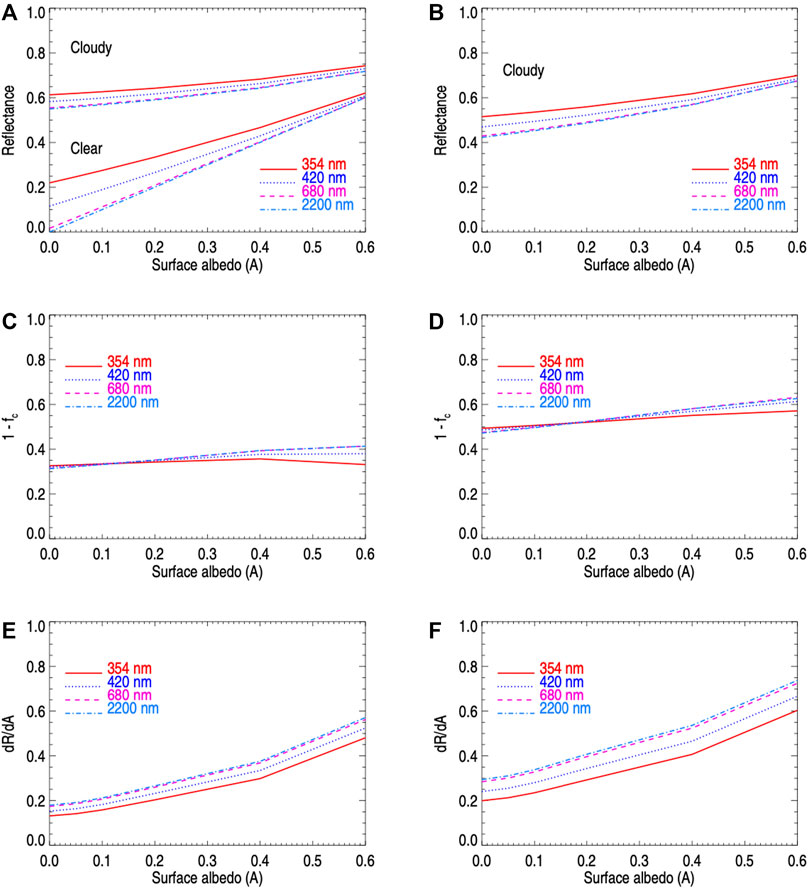
FIGURE 4. Radiative transfer calculations for nadir and solar zenith angle of 45° for an ice cloud model (left panels) and C1 model (right panels, see text for more detail) showing reflectance (R) for cloudy cases with cloud optical thicknesses of 10 in A and B (clear sky calculations also in panel A); one minus the effective cloud fraction, f_c, in C, D; and the sensitivity of the reflectance to a unit change in surface albedo (A), denoted dR/dA as a function of surface albedo for four wavelengths spanning the ultraviolet through short-wave infrared.

FIGURE 5

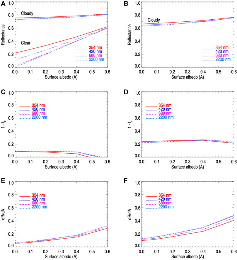
FIGURE 5. Similar to Figure 4 but for cloud optical thickness of 20.

Figures 4A,B, 5A,B show simulated observed reflectances in cloudy conditions (calculations for clear skies are shown in panels A) for four wavelengths spanning ultraviolet (UV) through short-wave infrared wavelengths (SWIR) (354 (UV), 420 (blue), 680 (red), and 2,200 (SWIR) nm) as a function of the surface albedo (A). As expected, the reflectances increase with decreasing wavelength owing to the effects of Rayleigh scattering and as shown in the GOME-2 spectra. For the clear sky simulations at the two longest wavelengths, the reflectance is nearly equal to the surface albedo as may be expected. The reflectances are seen to increase at all wavelengths with increasing surface albedo. Although this surface albedo dependence is smaller for a cloud optical thickness of 20, it is still present. This is an indication of sensitivity to the surface albedo.

We similarly show the quantity one minus the effective cloud fraction f_c in Figures 4C,D, 5C,D as a function of A. This quantity may be interpreted as the fraction of the observed raidance corresponding to a clear sky portion of the scene within the IPA MLER model. This fraction is about 30% for the ice cloud and 50% for the water cloud. Here, we see that f_c is fairly spectrally invariant, particularly for the visible through SWIR bands, as discussed in more detail below. The UV wavelength shows some deviations from wavelength invariance at higher surface albedos.

Figures 4E,F, 5E,F display the sensitivity of the reflectance (R) to the surface albedo (denoted dR/dA) as a function of A. The results show, as expected, higher sensitivity to the surface at higher surface albedos, a slight decrease in sensitivity with decreasing wavelength (owing to Rayleigh scattering), and slightly lower sensitivities for the ice cloud model as compared with the C1 model resulting from the different cloud phase functions. Values of the sensitivity can be interpreted approximately as the fractional change in observed reflectance resulting from a change in surface albedo. Sensitivities range from about 0.15 for the ice cloud model with low A to as high as 0.7 for high A for the C1 model in the τ = 10 case and from about 0.05 to 0.45 for the corresponding τ = 20 simulations. These results are consistent with a basic model of cloud transmittance given by Krotkov et al. (2001). Corresponding calculations for a view zenith angle of 40° are provided in the supplement.

3.4 Spatial Dependence

Figure 6A shows the observed all-sky red reflectance, ρ_R, on August 2, 2018 along with the reconstructed R_G2 (Figure 6B), the difference between the target and reconstructed R (R_M-R_G2, Figure 6C), and estimated R_G2 uncertainties from the NN fitting (Figure 6D). At this wavelength with typical non-desert land surface reflectances, a ρ_R of 0.4 corresponds approximately to cloud optical thickness, τ, of 5, ρ_R = 0.6 corresponds roughly to τ = 10, and ρ_R = 0.7 corresponds to τ = ∼ 20 (Kujanpää and Kalakoski, 2015). So even at high values of observed ρ_R, a small fraction of incoming sunlight reaches the surface and is then reflected from the surface and penetrates through the clouds to reach a satellite-borne sensor. Even though the fraction of surface-reflected light may be quite small, its spectral signature still may be distinguished from that of the clouds and atmosphere in observations with sufficient signal-to-noise ratios. The estimated R_G2 uncertainties shown in Figure 3D display generallly larger errors for more heavily clouded conditions as expected. In the presence of small amounts of undetected snow or ice within a GOME-2 pixel, R_G2 would likely be underestimated as the trained NN may confuse snow for clouds and subsequently try to reconstruct the snow- or ice-free part of the pixel, i.e., snow clearing.

FIGURE 6

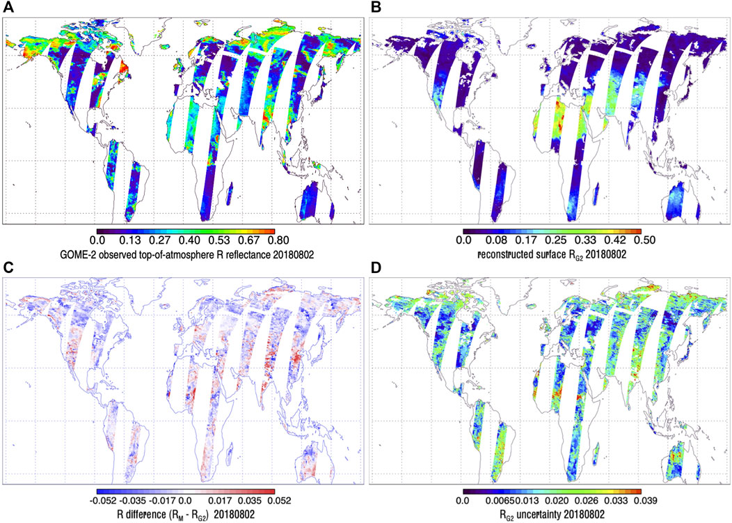
FIGURE 6. Results for GOME-2 red (R) reflectances on August 2, 2018: (A) GOME-2 original R reflectance (ρ_R) to show presence of clouds (generally higher reflectances) (B) reconstructed from GOME-2 (R_G2); (C) surface reflectance difference map, collocated MODIS MCD43 R_M minus R_G2; (D) estimated R_G2 uncertainties. Maps for (B–D) show only for GOME-2 pixels with observed red R $<$ 0.6.

Some R differences may result in part from the fact that the underlying MCD43 R_M is estimated using a moving weighted 16 days window and is not a true daily product. In addition, the MCD43 product may occasionally be affected by cloud and/or aerosol contamination or a small amount of available data.

Overall, R_G2 provides nearly complete coverage over the GOME-2 swaths, capturing the major spatial features in the R_M training data set. On this day, a global map of aerosol optical thickness from the NASA Global Modeling and Assimilation Office’s (GMAO’s) Modern-Era Retrospective Analysis for Research and Applications, Version 2 (MERRA-2) assimilation (Gelaro et al., 2017) shows high aerosol loading across northern Africa towards the Saudi Arabian peninsula and the Indian subcontinent as well as in southern Africa and the western United States. The absorbing aerosol index (AAI), an indicator of absorbing types of aerosol such as dust and smoke, derived from the Ozone Mapping and Profiler Suite (OMPS) on the Suomi National Polar Partnership (SNPP) satellite (Torres, 2019) shows high values across the Sahara $(>2)$ and MiddleEast (see supplement) presumably owing to the transport of dust. High AAI values are also seen over other areas, likely from smoke transported from fires including over southern Africa, the western US, and Siberia. Differences between target and predicted R are not substantially higher in these regions as compared with other areas, indicating that the training appears to work reasonably well in the presence of high absorbing aerosol loading.

Figure 7 shows GOME-2 all sky, reconstructed, and MCD43 target surface RGB images for August 2, 2018. GOME-2 pixels are substantially impacted by clouds as well as Rayleigh scattering. The GOME-2 atmospherically-corrected, nadir-adjusted, cloud-cleared reconstructed RGB image of the Earth’s land surface by eye is almost indistinguishable from that of the target MCD43 data. A close examination of the images shows some apparent artifacts in the reconstructed GOME-2 data on the easternmost part of the swath that crosses over southeast Asia. However, the GOME-2 data show a bit more uniformity in the surface RGB over the highly cloudy Indian subcontinent region. Note that to enhance the contrast, all RGB images shown here are selectively scaled using the IDL ScaleModis procedure supplied with the coyote library from Fanning Software Consulting that is based on code originally developed by the MODIS rapid response team for image display.

FIGURE 7

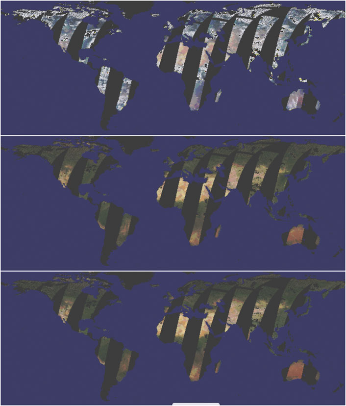
FIGURE 7. Top: GOME-2 RGB image from August 2, 2018; Middle: Reconstructed surface RGB image from GOME-2; Bottom: Surface RGB from MODIS MCD43 averaged over GOME-2 pixels. Snow/ice covered pixels are not masked out. Orbital gaps as well as pixels with reflectances $>$ 0.7 or not passing the reconstruction check are masked out. Ocean data are colored as blue and are not considered in this study.

We studied a sample of the outlier cases produced with GOME-2 that did not agree well with collocated MODIS data. In some of these, we found excess filling-in of solar Fraunhofer lines that is indicative of additive effects in the observed radiances as discussed by, e.g., Gorkavyi et al. (2021). Scattered light, dark current, non-linearity, bad or dead pixels, changes in the spectral response function from inhomogeneous slit illumination or temperature changes, eclipses, detector memory effects, saturation, and cloud three dimensional (3D) effects (light scattered from clouds or aerosol outside the area of the ground footprint) are examples of effects that may lead to additive radiance errors in GOME-2 and similar instruments (e.g., Lichtenberg et al., 2006; Gorkavyi et al., 2021). These additive error could in turn result in problems reconstructing surface reflectances from cloudy spectra and the artifacts seen by eye if not flagged by our quality control.

Figure 8 provides a zoomed in view of the Saharan region that was impacted by both dust and clouds. The whitish and grayish pixels in the top panel indicate cloud contamination, particularly in the lower right corner of the panels where ρ_R exceeds 0.6 and is removed from the images. Here, the increase in green vegetation towards the bottom of the lower two images can be seen clearly although some noise is present in the easternmost orbit at this transition which is also seen to be cloudy. Many of the details from the MODIS data are well captured by GOME-2 despite the heavy aerosol loading across the region that is present on this day. Additional RGB imagery for a date in a different season (February 1, 2018) is shown in the supplement where the NN has apparently performed snow clearing as well as cloud clearing along with the corresponding aerosol loading and AAI.

FIGURE 8

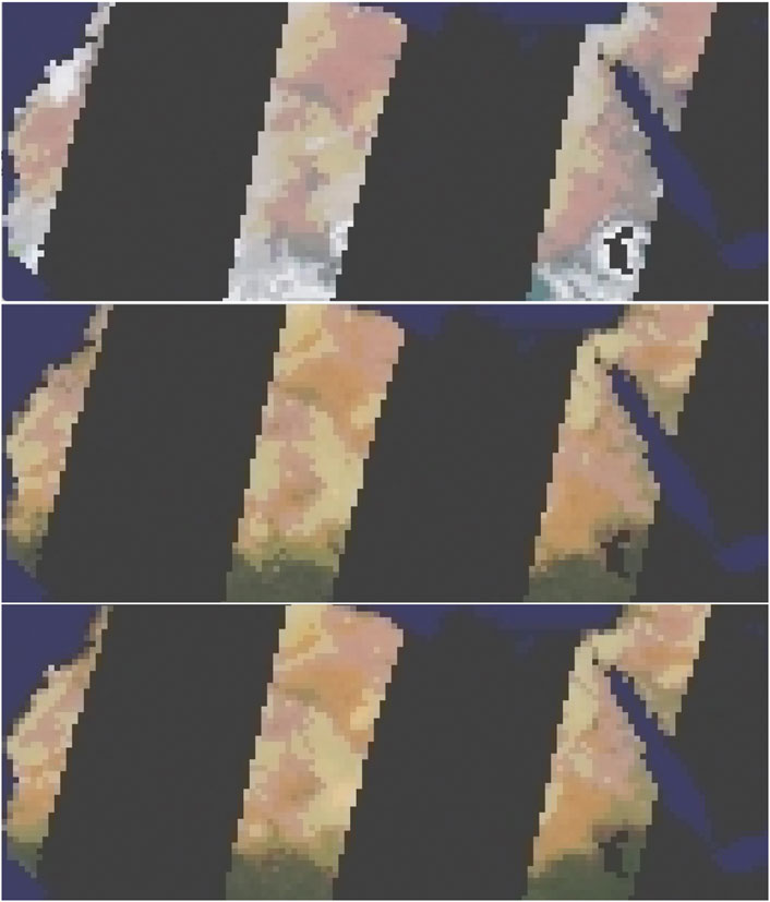
FIGURE 8. Similar to Figure 7 but zoomed in on northern Africa; Top: GOME-2 RGB image from August 2, 2018; Middle: Reconstructed surface RGB image from GOME-2; Bottom: Surface RGB from MODIS MCD43 averaged over GOME-2 pixels.

3.5 Temporal Dependence

We processed 1 year of GOME-2 data (2018) to analyze time series of the reconstructed reflectances at different sites. Our QA checks caught many but not all outliers. We therefore applied an additional simple outlier check by checking whether any points at a given location fell outside the range of the annual mean ±4 standard deviations. We selected locations near eddy covariance flux towers. Here we show one example and provide additional time series in the supplement.

Figure 9 shows one example over southeast Asia where there is substantial seasonal variability. The time series of the reconstructed RGBs are noisier in general than those of the collocated MCD43 target data. The reconstructed surface reflectances capture the overall seasonal variations from higher values at the beginning of the year through a transition to lower values at the middle to late part of the year. In this example, about 30% of data are filtered by the snow check, 4% by the high cloudiness check (here we allow data up to a red reflectance of 0.7), and 0% by the reconstruction check. One low value around day 103 is not flagged by the four standard deviation check (possibly due to unflagged snow) but could be detected by a more sophisticated time series continuity check. Examples in the supplement show a few cases of possible cloud contamination in the MODIS target data used for training and evaluation.

FIGURE 9

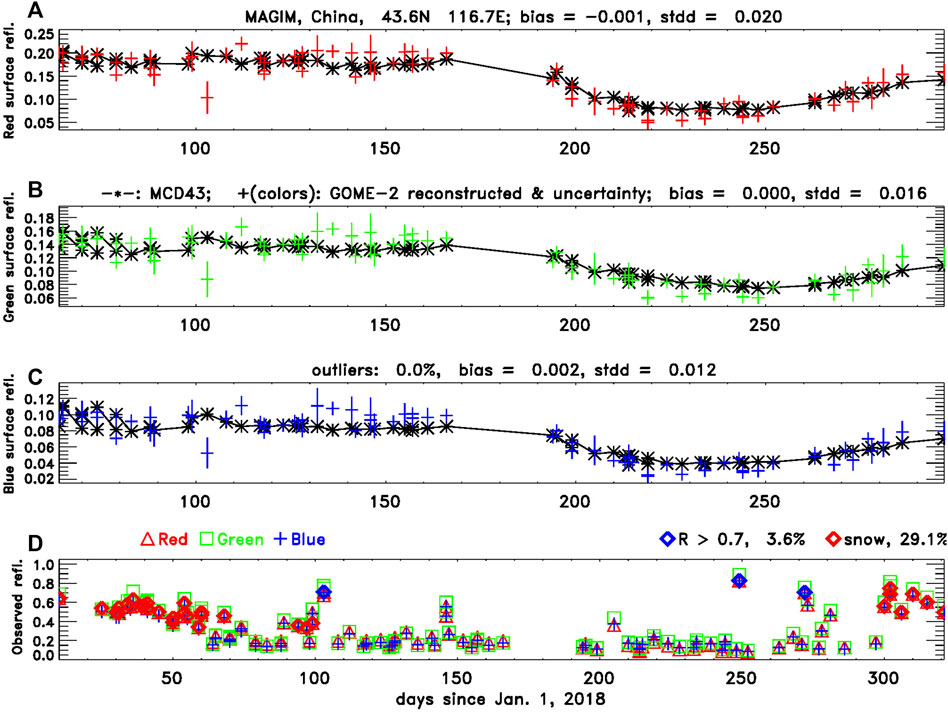
FIGURE 9. Time series near the MAGIM eddy covariance site in China of target (MCD43, black line with stars) and reconstructed surface reflectances (GOME-2: colored + with extended lines in the y direction to indicate the one standard deviation uncertainty) for (A) Red; (B) Green; and (C) Blue bands, and (D) Observed reflectances from GOME-2 pixels. Bias and standard deviation of the reconstructed reflectances with respect to the target are provided for each band (color). The number of outliers found by the four standard deviation outlier check is indicated in (C) (in this case zero). Points filtered by the quality assurance (QA) checks are given in (D) including snow (red diamonds), extremely high cloudiness (blue diamonds), or poorly reconstructed spectra from the leading 14 principal components (none in this case).

3.6 Interpretation of NN Learning Within the MLER Framework

Gupta et al. (2016) conducted 1D radiative transfer simulations in complex cloudy conditions using three different cloud models and a range of geometrical cloud fractions to show that f_c is fairly wavelength invariant over a large spectral range from the UV to the NIR. We show additional supporting calculations in Figures 4C,D, 5C,D. The near wavelength invariance of f_c implies that in the absence of gaseous, cloud, or aerosol absorption, the radiative transfer in a complex scene can be modeled with approximately one parameter: f_c. If f_c, and its relatively small wavelength dependence, can be distinguished from the spectral dependence of the underlying surface, then it is possible to reconstruct a surface RGB image in cloudy conditions. We have utilized machine learning to accomplish this task with a large, representative training set. We may then compute f_c at the training wavelengths using the reconstructed reflectances as described above and examine its wavelength dependence.

Figure 10A shows f_c derived at the red wavelength band. Note that here we have used the reconstructed NBAR as a proxy for the LER. A more exact estimate of f_c should account for the BRDF-dependence of the reflectance (Vasilkov et al., 2017; Vasilkov et al., 2018). For our purpose of roughly estimating f_c and its wavelength dependence, use of the reconstructed NBAR as the surface LER should suffice; however, note that neglect of the surface BRDF may contribute to wavelength and cross track dependence in f_c. Figure 10B shows the difference between f_c computed for the red and blue wavelengths.

FIGURE 10

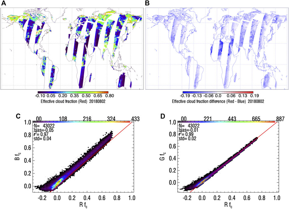
FIGURE 10. f_c computed at different wavelengths from August 2, 2018 GOME-2 data: (A) f_c computed at the red band wavelength; (B) map of difference between computed f_c at red and blue wavelengths; (C) density plot of f_c at red and blue wavelengths; (D) density plot of f_c at red and green wavelengths. The red line in panels (C) and (D) is the 1:1 line.

Larger spread and bias is seen in the comparison of f_c from red and blue wavelengths in Figure 10C as compared with red and green wavelengths in Figure 10D. There is only a small mean difference of 0.01 between f_c at red and green wavelengths. Rayleigh scattering, which is much stronger at blue wavelengths, reduces the effects of cloud shadowing as well as cloud and surface bi-directional effects, causing larger differences between red and blue wavelength f_c. Negative values are shown here and may be due to a combination of factors including shadowing, unaccounted for effects of absorbing aerosol, and GOME-2 calibration error. GOME-2A is known to have suffered from radiometric degradation (Munro et al., 2016). The NN training is able to adjust for absolute calibration error in GOME-2 relative to MODIS. The slight improvement in results obtained when angles are used as predictors may result from better ability to adjust for any remaining geometrically-dependent biases.

The near wavelength invariance of f_c provides an explanation of how the NN is able to separate the surface and cloud spectral signatures by extracting f_c, or similar information, and its relatively small wavelength dependence. The near spectral invariance of f_c shown in our radiative transfer calculations (Figures 4C,D, 5C,D), also suggests that our cloud-clearing method may be able to fill spectral gaps in the RGB training data set in order to estimate more complex surface spectral signatures such as from chlorophyll absorption. Finally, this example gives an indication as to why the errors in the reconstructed RGBs are correlated; an error in the derived f_c should produce spectrally correlated errors in estimated surface reflectances. Other works have similarly exploited the spectral differences between ocean surface reflectance and spectrally smooth clouds, aerosol, and ocean glint (e.g., Steinmetz et al., 2011; Frouin et al., 2014; Frouin and Gross-Colzy, 2016, and references therein).

4 Discussion and Conclusion

We have provided an approach to reconstruct RGB imagery in moderately cloudy and aerosol-contaminated conditions using hyperspectral imagery. Our approach employs a NN trained on an appropriate sample of data. In a scattering atmosphere, surface spectral effects are present in satellite-observed spectra and the machine learning algorithm appears able to separate surface spectral fingerprints from those of cloud, aerosol, and atmospheric scattering and absorption and to account for the presence of cloud and vegetation shadowing. Once trained, the NN estimates the surface reflectances simply and efficiently, requiring only a few matrix muliplications and applications of non-linear functions for each processed spectrum.

We stress that the success of the method depends critically on the quality of the training data set. In this study, we utilize high quality daily NBARs that can be accurately averaged over a larger GOME-2 pixel. An advantage of our approach is that a large training sample can be constructed over a wide range of conditions; it does not depend upon simulating a multitude of situations for training including the complex conditions that occur with real observations. Our approach is also robust in the presence of relative calibration error. However, we note that for application to other higher spatial resolution instruments, similar high quality training data may not be available. Joiner et al. (2021) apply a variation of the approach described here to a case study from a higher spatial resolution imager for a scene in which parts of the image are visibly obscured by clouds. Instead of using MODIS data for training, they use a clear sky image taken a short time before a cloudy image with the assumption that the surface reflectance remains constant during that time. They show that under the conditions of their case study scene, many surface details are recovered with a relatively small amount of image smearing. In that study, it was not clear how much of the spatial smearing resulted from instrumental artifacts and geophysical effects.

While cloud and aerosol 3D effects are less common in large pixel sensors such as GOME-2 as compared with higher resolution imagers such as MODIS, they may occur under certain conditions and lead to additive errors. In cases of broken but optically thick clouds with a homogeneous surface underneath, GOME-2 may be able to reconstruct the surface reflectance from the clear parts of a scene. However, for imagers that resolve such clouds, the signals from underneath thick clouds may be spectrally and spatially scrambled, leading to a spatially smeared reconstructed image. Future studies will apply similar approaches to other higher spatial resolution imagers under a greater variety of conditions. Ultimately, the results of such studies will help to determine whether our spectral image reconstruction approach will be accurate enough for a given application under different conditions.

There are a host of potential applications of the approach developed here to extract information about the Earth’s surface, over both land and ocean. This study focuses on land surfaces; subsequent studies will address the ocean surface. We plan to test the approach with other higher order level 2 data products as target output variables. The desired precision and accuracy as well as availability of adequate training data sets will be considerations that factor into whether or not this approach will be feasible for a given application.

While our approach was implemented with GOME-2 that provides complete spectral coverage from the UV through NIR, there will be many more instruments available for such applications in the future that have enhanced capabilities. For example, the results obtained here are applicable to PACE and other hyper-spectral instruments that will provide substantially higher spatial resolution. The NASA geostationary tropospheric emissions: monitoring of pollution (TEMPO) (Zoogman et al., 2017) (expected launch in the 2023 time frame) will provide nearly complete spectral coverage of UV through part of the red edge (740 nm) over much of North America at an hourly time step at ∼5 km spatial resolution. Other instruments to be launched over the next several years may provide spectral coverage appropriate for certain applications. For example, the European Space Agency (ESA) FLuORescence Imaging Spectrometer (FLORIS) on the FLuorescence EXplorer (FLEX) mission will fly in low Earth orbit with approximately 300 m spatial resolution and spectral coverage from 500 to 780 nm (i.e., green through NIR) over a 250 km swath (Coppo et al., 2017). The NASA surface biology and geology (SBG) and the German Environmental Mapping and Analysis Program (EnMAP) (Storch et al., 2020) will produce hyper-spectral imagery using wavelengths from the visible through SWIR. These instruments are particularly well suited for applications related to land biochemical processes. The methods developed here are also applicable to hyper-spectral imagery acquired by instruments on the international space station as well as aircraft and other suborbital platforms.

Data Availability Statement

The original contributions presented in the study are included in the article/Supplementary Material, further inquiries can be directed to the corresponding author.

Author Contributions

JJ was responsible for the design of the methodology, investigation, and formal analysis, and wrote the first draft of the article. JJ, AV, and NK contributed to the conceptualization. JJ, AV, ZF, and WQ contributed to the software and calculations. JJ, AV, and NK provided overall supervision of the project. NK and JJ contributed to funding acquisition. JJ, CL, and LL contributed to data curation. JJ and YY contributed to visualization. All authors contributed to article revision, read, and approved the submitted version.

Funding

This work was supported in part by the NASA through the Arctic–Boreal Vulnerability Experiment (ABoVE) as well as the OMI, PACE, and TEMPO science team programs.

Conflict of Interest

Authors ZF, WQ, YY, and AV were employed by the company Science Systems and Applications, Inc. (SSAI).

The remaining authors declare that the research was conducted in the absence of any commercial or financial relationships that could be construed as a potential conflict of interest.

Publisher’s Note

All claims expressed in this article are solely those of the authors and do not necessarily represent those of their affiliated organizations, or those of the publisher, the editors and the reviewers. Any product that may be evaluated in this article, or claim that may be made by its manufacturer, is not guaranteed or endorsed by the publisher.

Acknowledgments

We are particularly grateful to the EUMETSAT for providing GOME-2 data and NASA and the MCD43 team for providing the MODIS surface reflectance data set. We thank all those who contributed to the excellent calibration of these instruments and to the teams that provided the data sets used here including the NASA OMPS science team for provide aerosol index maps, the GMAO’s aerosol assimilation group, and the National Snow and Ice Data Center (NSIDC) for providing snow and ice data. The lead author thanks P. K. Bhartia, A. da Silva, L. Remer, and two reviewers for enlightening comments that helped to improve the article.

Supplementary Material

The Supplementary Material for this article can be found online at: https://www.frontiersin.org/articles/10.3389/frsen.2021.716430/full#supplementary-material

References

AghaKouchak, A., Farahmand, A., Melton, F. S., Teixeira, J., Anderson, M. C., Wardlow, B. D., et al. (2015). Remote Sensing of Drought: Progress, Challenges and Opportunities. Rev. Geophys. 53, 452–480. doi:10.1002/2014RG000456

CrossRef Full Text | Google Scholar

Ahmad, Z., Bhartia, P. K., and Krotkov, N. (2004). Spectral Properties of Backscattered UV Radiation in Cloudy Atmospheres. J. Geophys. Res. 109, 1. doi:10.1029/2003JD003395

CrossRef Full Text | Google Scholar

Anyamba, A., and Tucker, C. J. (2012). “Historical Perspectives on AVHRR NDVI and Vegetation Drought Monitoring,” in Remote Sensing of Drought: Innovative Monitoring Approaches. Editors B. D. Wardlow, M. C. Anderson, and J. P. Verdin (CRC Press/Taylor & Francis).

Google Scholar

Banks, A. C., and Mélin, F. (2015). An Assessment of Cloud Masking Schemes for Satellite Ocean Colour Data of marine Optical Extremes. Int. J. Remote Sensing 36, 797–821. doi:10.1080/01431161.2014.1001085

CrossRef Full Text | Google Scholar

Baum, B. A., Yang, P., Heymsfield, A. J., Bansemer, A., Cole, B. H., Merrelli, A., et al. (2014). Ice Cloud Single-Scattering Property Models with the Full Phase Matrix at Wavelengths from 0.2 to 100µm. J. Quantitative Spectrosc. Radiative Transfer 146, 123–139. doi:10.1016/j.jqsrt.2014.02.029

CrossRef Full Text | Google Scholar

Brodzik, M. J., and Stewart, J. S. (2016). Near-Real-Time SSM/I-SSMIS EASE-Grid Daily Global Ice Concentration and Snow Extent, Version 5, Snow Extent. Boulder, CO: National Snow and Ice Data Center Distributed Active Archive Center. doi:10.5067/3KB2JPLFPK3R

CrossRef Full Text | Google Scholar

Claverie, M., Ju, J., Masek, J. G., Dungan, J. L., Vermote, E. F., Roger, J.-C., et al. (2018). The Harmonized Landsat and Sentinel-2 Surface Reflectance Data Set. Remote Sensing Environ. 219, 145–161. doi:10.1016/j.rse.2018.09.002

CrossRef Full Text | Google Scholar

Coppo, P., Taiti, A., Pettinato, L., Francois, M., Taccola, M., and Drusch, M. (2017). Fluorescence Imaging Spectrometer (FLORIS) for ESA FLEX Mission. Remote Sensing 9, 649. doi:10.3390/rs9070649

CrossRef Full Text | Google Scholar

Deirmendjian, D. (1969). Electromagnetic Scattering on Spherical Polydispersions. New York): Elsevir Sci., 290.

Google Scholar

Diner, D. J., Martonchik, J. V., Kahn, R. A., Pinty, B., Gobron, N., Nelson, D. L., et al. (2005). Using Angular and Spectral Shape Similarity Constraints to Improve MISR Aerosol and Surface Retrievals over Land. Remote Sensing Environ. 94, 155–171. doi:10.1016/j.rse.2004.09.009

CrossRef Full Text | Google Scholar

Duchemin, B., and Maisongrande, P. (2002). Normalisation of Directional Effects in 10-day Global Syntheses Derived from VEGETATION/SPOT:. Remote Sensing Environ. 81, 90–100. doi:10.1016/S0034-4257(01)00336-4

CrossRef Full Text | Google Scholar

Frouin, R., Duforêt, L., and Steinmetz, F. (2014). “Atmospheric Correction of Satellite Ocean-Color Imagery in the Presence of Semi-transparent Clouds,” in Ocean Remote Sensing and Monitoring from Space, Beijing, China. Editors R. J. Frouin, D. Pan, and H. Murakami (Bellingham, WA: International Society for Optics and Photonics (SPIE)), 47–61. doi:10.1117/12.2074008

CrossRef Full Text | Google Scholar

Frouin, R. J., Franz, B. A., Ibrahim, A., Knobelspiesse, K., Ahmad, Z., Cairns, B., et al. (2019). Atmospheric Correction of Satellite Ocean-Color Imagery during the PACE Era. Front. Earth Sci. 7, 145. doi:10.3389/feart.2019.00145

PubMed Abstract | CrossRef Full Text | Google Scholar

Frouin, R. J., and Gross-Colzy, L. S. (2016). “Contribution of Ultraviolet and Shortwave Infrared Observations to Atmospheric Correction of PACE Ocean-Color Imagery,” in Remote Sensing of the Oceans and Inland Waters: Techniques, Applications, and Challenges, New Delhi, India. Editors R. J. Frouin, S. C. Shenoi, and K. H. Rao (Bellingham, WA: International Society for Optics and Photonics (SPIE)), 35–46. doi:10.1117/12.2229891

CrossRef Full Text | Google Scholar

Gelaro, R., McCarty, W., Suárez, M. J., Todling, R., Molod, A., Takacs, L., et al. (2017). The Modern-Era Retrospective Analysis for Research and Applications, Version 2 (MERRA-2). J. Clim. 30, 5419–5454. doi:10.1175/JCLI-D-16-0758.1

PubMed Abstract | CrossRef Full Text | Google Scholar

Gorkavyi, N., Fasnacht, Z., Haffner, D., Marchenko, S., Joiner, J., and Vasilkov, A. (2021). Detection of Anomalies in the UV-Vis Reflectances from the Ozone Monitoring Instrument. Atmos. Meas. Tech. 14, 961–974. doi:10.5194/amt-14-961-2021

CrossRef Full Text | Google Scholar

Govaerts, Y. M., Lattanzio, A., Pinty, B., and Schmetz, J. (2004). Consistent Surface Albedo Retrieval from Two Adjacent Geostationary Satellites. Geophys. Res. Lett. 31, 1. doi:10.1029/2004GL020418

CrossRef Full Text | Google Scholar

Groom, S., Sathyendranath, S., Ban, Y., Bernard, S., Brewin, R., Brotas, V., et al. (2019). Satellite Ocean Colour: Current Status and Future Perspective. Front. Mar. Sci. 6, 485. doi:10.3389/fmars.2019.00485

CrossRef Full Text | Google Scholar

Gross-Colzy, L., Colzy, S., Frouin, R., and Henry, P. (2007b). “A General Ocean Color Atmospheric Correction Scheme Based on Principal Components Analysis: Part II. Level 4 Merging Capabilities,” in Coastal Ocean Remote Sensing. Editors R. J. Frouin, and Z. Lee (Bellingham, WA: International Society for Optics and Photonics (SPIE)), 21–32. doi:10.1117/12.738514

CrossRef Full Text | Google Scholar

Gross-Colzy, L., Colzy, S., Frouin, R., and Henry, P. (2007a). “A General Ocean Color Atmospheric Correction Scheme Based on Principal Components Analysis: Part I. Performance on Case 1 and Case 2 Waters,” in Coastal Ocean Remote Sensing. Editors R. J. Frouin, and Z. Lee (Bellingham, WA: International Society for Optics and Photonics (SPIE)), 9–20. doi:10.1117/12.738508

CrossRef Full Text | Google Scholar

Gupta, P., Joiner, J., Vasilkov, A., and Bhartia, P. K. (2016). Top-of-the-atmosphere Shortwave Flux Estimation from Satellite Observations: an Empirical Neural Network Approach Applied with Data from the A-Train Constellation. Atmos. Meas. Tech. 9, 2813–2826. doi:10.5194/amt-9-2813-2016

CrossRef Full Text | Google Scholar

He, T., Zhang, Y., Liang, S., Yu, Y., and Wang, D. (2019). Developing Land Surface Directional Reflectance and Albedo Products from Geostationary GOES-R and Himawari Data: Theoretical Basis, Operational Implementation, and Validation. Remote Sensing 11, 2655. doi:10.3390/rs11222655

CrossRef Full Text | Google Scholar

Joiner, J., Fasnacht, Z., Gao, B.-C., and Qin, W. (2021). Use of Multi-Spectral Visible and Near-Infrared Satellite Data for Timely Estimates of the Earth’s Surface Reflectance in Cloudy and Aerosol Loaded Conditions: Part 2 - Image Restoration with HICO Satellite Data in Overcast Conditions. Frontiers in Remote Sensing 2. doi:10.3389/frsen.2021.721957

CrossRef Full Text | Google Scholar

Joiner, J., and Yoshida, Y. (2020). Satellite-based Reflectances Capture Large Fraction of Variability in Global Gross Primary Production (GPP) at Weekly Time Scales. Agric. For. Meteorology 291, 108092. doi:10.1016/j.agrformet.2020.108092

CrossRef Full Text | Google Scholar

Joiner, J., Yoshida, Y., Zhang, Y., Duveiller, G., Jung, M., Lyapustin, A., et al. (2018). Estimation of Terrestrial Global Gross Primary Production (GPP) with Satellite Data-Driven Models and Eddy Covariance Flux Data. Remote Sensing 10, 1346. doi:10.3390/rs10091346

CrossRef Full Text | Google Scholar

Krotkov, N. A., Herman, J. R., Bhartia, P. K., Fioletov, V., and Ahmad, Z. (2001). Satellite Estimation of Spectral Surface UV Irradiance: 2. Effects of Homogeneous Clouds and Snow. J. Geophys. Res. 106, 11743–11759. doi:10.1029/2000jd900721

CrossRef Full Text | Google Scholar

Kujanpää, J., and Kalakoski, N. (2015). Operational Surface UV Radiation Product from GOME-2 and AVHRR/3 Data. Atmos. Meas. Tech. 8, 4399–4414. doi:10.5194/amt-8-4399-2015

CrossRef Full Text | Google Scholar

Lary, D. J., Alavi, A. H., Gandomi, A. H., and Walker, A. L. (2016). Machine Learning in Geosciences and Remote Sensing. Geosci. Front. 7, 3–10. doi:10.1016/j.gsf.2015.07.003

CrossRef Full Text | Google Scholar

Li, S., Wang, W., Hashimoto, H., Xiong, J., Vandal, T., Yao, J., et al. (2019a). First Provisional Land Surface Reflectance Product from Geostationary Satellite Himawari-8 AHI. Remote Sensing 11, 2990. doi:10.3390/rs11242990

CrossRef Full Text | Google Scholar

Li, Z., Shen, H., Cheng, Q., Li, W., and Zhang, L. (2019b). Thick Cloud Removal in High-Resolution Satellite Images Using Stepwise Radiometric Adjustment and Residual Correction. Remote Sensing 11, 1925. doi:10.3390/rs11161925

CrossRef Full Text | Google Scholar

Lichtenberg, G., Kleipool, Q., Krijger, J. M., van Soest, G., van Hees, R., Tilstra, L. G., et al. (2006). SCIAMACHY Level 1 Data: Calibration Concept and In-Flight Calibration. Atmos. Chem. Phys. 6, 5347–5367. doi:10.5194/acp-6-5347-2006

CrossRef Full Text | Google Scholar

Lyapustin, A. I., Wang, Y., Laszlo, I., Hilker, T., G.Hall, F., Sellers, P. J., et al. (2012). Multi-angle Implementation of Atmospheric Correction for MODIS (MAIAC): 3. Atmospheric Correction. Remote Sensing Environ. 127, 385–393. doi:10.1016/j.rse.2012.09.002

CrossRef Full Text | Google Scholar

Lyapustin, A., Martonchik, J., Wang, Y., Laszlo, I., and Korkin, S. (2011a). Multiangle Implementation of Atmospheric Correction (MAIAC): 1. Radiative Transfer Basis and Look-Up Tables. J. Geophys. Res. Atmospheres 116, 1. doi:10.1029/2010JD014985.D03210

CrossRef Full Text | Google Scholar

Lyapustin, A., Wang, Y., Laszlo, I., Kahn, R., Korkin, S., Remer, L., et al. (2011b). Multiangle Implementation of Atmospheric Correction (MAIAC): 2. Aerosol Algorithm. J. Geophys. Res. Atmospheres 116, 1. doi:10.1029/2010JD014986.D03211

CrossRef Full Text | Google Scholar

Ma, L., Liu, Y., Zhang, X., Ye, Y., Yin, G., and Johnson, B. A. (2019). Deep Learning in Remote Sensing Applications: A Meta-Analysis and Review. ISPRS J. Photogrammetry Remote Sensing 152, 166–177. doi:10.1016/j.isprsjprs.2019.04.015

CrossRef Full Text | Google Scholar

Maignan, F., Bréon, F.-M., and Lacaze, R. (2004). Bidirectional Reflectance of Earth Targets: Evaluation of Analytical Models Using a Large Set of Spaceborne Measurements with Emphasis on the Hot Spot. Remote Sensing Environ. 90, 210–220. doi:10.1016/j.rse.2003.12.006

CrossRef Full Text | Google Scholar

Maxwell, A. E., Warner, T. A., and Fang, F. (2018). Implementation of Machine-Learning Classification in Remote Sensing: an Applied Review. Int. J. Remote Sensing 39, 2784–2817. doi:10.1080/01431161.2018.1433343

CrossRef Full Text | Google Scholar

Mehta, A., Sinha, H., Mandal, M., and Narang, P. (2021). “Domain-Aware Unsupervised Hyperspectral Reconstruction for Aerial Image Dehazing,” in 2021 IEEE Winter Conference on Applications of Computer Vision (WACV), 413–422. doi:10.1109/WACV48630.2021.00046

CrossRef Full Text | Google Scholar

Mercury, M., Green, R., Hook, S., Oaida, B., Wu, W., Gunderson, A., et al. (2012). Global Cloud Cover for Assessment of Optical Satellite Observation Opportunities: A HyspIRI Case Study. Remote Sensing Environ. 126, 62–71. doi:10.1016/j.rse.2012.08.007

CrossRef Full Text | Google Scholar

Muller, J.-P., Zuhlke, M., Brockmann, C., Preusker, R., Fischer, J., and Regner, P. (2007). “ALBEDOMAP: MERIS Land Surface Albedo Retrieval Using Data Fusion with MODIS BRDF and its Validation Using Contemporaneous EO and In Situ Data Products,” in 2007 IEEE International Geoscience and Remote Sensing Symposium (IEEE), 2404–2407. doi:10.1109/IGARSS.2007.4423326

CrossRef Full Text | Google Scholar

Munro, R., Lang, R., Klaes, D., Poli, G., Retscher, C., Lindstrot, R., et al. (2016). The GOME-2 Instrument on the Metop Series of Satellites: Instrument Design, Calibration, and Level 1 Data Processing - an Overview. Atmos. Meas. Tech. 9, 1279–1301. doi:10.5194/amt-9-1279-2016

CrossRef Full Text | Google Scholar

Qin, W., Fasnacht, Z., Haffner, D., Vasilkov, A., Joiner, J., Krotkov, N., et al. (2019). A Geometry-dependent Surface Lambertian-Equivalent Reflectivity Product for UV-Vis Retrievals - Part 1: Evaluation over Land Surfaces Using Measurements from OMI at 466 Nm. Atmos. Meas. Tech. 12, 3997–4017. doi:10.5194/amt-12-3997-2019

CrossRef Full Text | Google Scholar

Schaaf, C. B., Gao, F., Strahler, A. H., Lucht, W., Li, X., Tsang, T., et al. (2002). First Operational BRDF, Albedo Nadir Reflectance Products from MODIS. Remote Sensing Environ. 83, 135–148. doi:10.1016/S0034-4257(02)00091-3

CrossRef Full Text | Google Scholar

Schaaf, C. (2015). MCD43C4 MODIS/Terra+Aqua BRDF-Adjusted Nadir Reflectance Daily L3 Global 0.05◦ CMG V006. Sioux Falls, SD: NASA EOSDIS Land Processes DAAC. doi:10.5067/MODIS/MCD43C4.006

CrossRef Full Text | Google Scholar

Schroeder, T., Behnert, I., Schaale, M., Fischer, J., and Doerffer, R. (2007). Atmospheric Correction Algorithm for MERIS above Case‐2 Waters. Int. J. Remote Sensing 28, 1469–1486. doi:10.1080/01431160600962574

CrossRef Full Text | Google Scholar

Spurr, R. J. D. (2006). VLIDORT: A Linearized Pseudo-spherical Vector Discrete Ordinate Radiative Transfer Code for Forward Model and Retrieval Studies in Multilayer Multiple Scattering media. J. Quantitative Spectrosc. Radiative Transfer 102, 316–342. doi:10.1016/j.jqsrt.2006.05.005

CrossRef Full Text | Google Scholar

Stammes, P., Sneep, M., de Haan, J. F., Veefkind, J. P., Wang, P., and Levelt, P. F. (2008). Effective Cloud Fractions from the Ozone Monitoring Instrument: Theoretical Framework and Validation. J. Geophys. Res. 113, 1. doi:10.1029/2007JD008820

CrossRef Full Text | Google Scholar

Steinmetz, F., Deschamps, P.-Y., and Ramon, D. (2011). Atmospheric Correction in Presence of Sun Glint: Application to MERIS. Opt. Express 19, 9783–9800. doi:10.1364/OE.19.009783

PubMed Abstract | CrossRef Full Text | Google Scholar

Storch, T., Honold, H.-P., Alonso, K., Pato, M., Mücke, M., Basili, P., et al. (2020). Status of the Imaging Spectroscopy mission Enmap with Radiometric Calibration and Correction. ISPRS Ann. Photogramm. Remote Sens. Spat. Inf. Sci. 2020, 41–47. doi:10.5194/isprs-annals-V-1-2020-41-2020

CrossRef Full Text | Google Scholar

Torres, O. (2019). OMPS-NPP L2 NM Aerosol Index Swath Orbital V2, Greenbelt, MD, USA. Greenbelt, MD: Goddard Earth Sciences Data and Information Services Center (GES DISC). doi:10.5067/40L92G8144IV

CrossRef Full Text | Google Scholar

U.S. National Ice Center (2008). IMS Daily Northern Hemisphere Snow and Ice Analysis at 1 Km, 4 Km, and 24 Km Resolutions. Version 1. Boulder, CO: National Snow and Ice Data Center. doi:10.7265/N52R3PMC

CrossRef Full Text | Google Scholar

Vasilkov, A., Qin, W., Krotkov, N., Lamsal, L., Spurr, R., Haffner, D., et al. (2017). Accounting for the Effects of Surface BRDF on Satellite Cloud and Trace-Gas Retrievals: a New Approach Based on Geometry-dependent Lambertian Equivalent Reflectivity Applied to OMI Algorithms. Atmos. Meas. Tech. 10, 333–349. doi:10.5194/amt-10-333-2017

CrossRef Full Text | Google Scholar

Vasilkov, A., Yang, E.-S., Marchenko, S., Qin, W., Lamsal, L., Joiner, J., et al. (2018). A Cloud Algorithm Based on the O2-O2 477 Nm Absorption Band Featuring an Advanced Spectral Fitting Method and the Use of Surface Geometry-dependent Lambertian-Equivalent Reflectivity. Atmos. Meas. Tech. 11, 4093–4107. doi:10.5194/amt-11-4093-2018

CrossRef Full Text | Google Scholar

Wang, T., Shi, J., Letu, H., Ma, Y., Li, X., and Zheng, Y. (2019). Detection and Removal of Clouds and Associated Shadows in Satellite Imagery Based on Simulated Radiance fields. J. Geophys. Res. Atmos. 124, 7207–7225. doi:10.1029/2018JD029960

CrossRef Full Text | Google Scholar

Wang, Z., Schaaf, C. B., Sun, Q., Shuai, Y., and Román, M. O. (2018). Capturing Rapid Land Surface Dynamics with Collection V006 MODIS BRDF/NBAR/Albedo (MCD43) Products. Remote Sensing Environ. 207, 50–64. doi:10.1016/j.rse.2018.02.001

CrossRef Full Text | Google Scholar

Werdell, P. J., Behrenfeld, M. J., Bontempi, P. S., Boss, E., Cairns, B., Davis, G. T., et al. (2019). The Plankton, Aerosol, Cloud, Ocean Ecosystem mission: Status, Science, Advances. Bull. Am. Meteorol. Soc. 100, 1775–1794. doi:10.1175/BAMS-D-18-0056.1

CrossRef Full Text | Google Scholar

Yuan, W., Cai, W., Xia, J., Chen, J., Liu, S., Dong, W., et al. (2014). Global Comparison of Light Use Efficiency Models for Simulating Terrestrial Vegetation Gross Primary Production Based on the LaThuile Database. Agric. For. Meteorology 192-193, 108–120. doi:10.1016/j.agrformet.2014.03.007

CrossRef Full Text | Google Scholar

Zhang, L., Zhang, M., Sun, X., Wang, L., and Cen, Y. (2018). Cloud Removal for Hyperspectral Remotely Sensed Images Based on Hyperspectral Information Fusion. Int. J. Remote Sensing 39, 6646–6656. doi:10.1080/01431161.2018.1466068

CrossRef Full Text | Google Scholar

Zhu, X. X., Tuia, D., Mou, L., Xia, G.-S., Zhang, L., Xu, F., et al. (2017). Deep Learning in Remote Sensing: A Comprehensive Review and List of Resources. IEEE Geosci. Remote Sens. Mag. 5, 8–36. doi:10.1109/MGRS.2017.2762307

CrossRef Full Text | Google Scholar

Zoogman, P., Liu, X., Suleiman, R. M., Pennington, W. F., Flittner, D. E., Al-Saadi, J. A., et al. (2017). Tropospheric Emissions: Monitoring of Pollution (TEMPO). J. Quantitative Spectrosc. Radiative Transfer 186, 17–39. doi:10.1016/j.jqsrt.2016.05.008

PubMed Abstract | CrossRef Full Text | Google Scholar