A neural network approach to the estimation of in-water attenuation to absorption ratios from PACE mission measurements

1 Introduction

Plankton, Aerosol, Cloud, ocean Ecosystem (PACE) is a NASA Earth-observing satellite mission that, in the words of the mission’s official website, “[...] will help us [...] understand how the ocean and atmosphere exchange carbon dioxide,” “[...] will reveal how aerosols might fuel phytoplankton growth in the surface ocean,” and “will extend and expand NASA’s long-term observations of our living planet” (NASA PACE, 2022a). The mission science objectives, as further stated on the PACE mission website (NASA PACE, 2022b), include extending key systematic ocean biological, ecological, and biogeochemical climate data records and cloud and aerosol climate records, as well as improving our understanding of how aerosols influence ocean biogeochemical cycles and ecosystems and how ocean biological and photochemical processes affect the atmosphere. Polarization of light will be at the core of the mission, with two multi-angular polarimeters being included onboard the satellite: the SPEXone and HARP2 instruments. The latter in particular is a wide-swath polarimeter, with a field of view of 94° cross track; ±57° along track for four wavelengths (441, 549, 669, 873 nm), of which the first three are narrow band (15, 12, 16 nm respectively) and are of interest in this study. The instrument will allow the measurement of polarization at 60 along track viewing angles for the 669 nm band, and at 10 along track viewing for the others (NASA PACE, 2022c). Polarization is an important observable in Earth remote sensing, as it is recognized to be affected by the physical and optical properties of particles suspended both in the atmosphere and the oceans as light travels through air and water (Mishchenko et al., 2004; Chami and Platel, 2007; Lotsberg and Stamnes, 2010; Knobelspiesse et al., 2011; Chowdhary et al., 2012; Ibrahim et al., 2016). Consequently, polarization measurements in conjunction with traditional radiometric measurements are increasingly being treated as a crucial direction for remote sensing research (Jamet et al., 2019). The polarization of light is most frequently used to characterize aerosols (Mishchenko and Travis, 1997): this is due to the fact that upwelling light from the ocean is in general weaker, not only because of the substantially smaller relative refractive indices of hydrosols compared to aerosols, but also because of the effect of Snell’s window, whereby highly polarized light with a maximum near the critical angle undergoes total reflection and is partially prevented from leaving the water (Gilerson et al., 2020). Nevertheless, studies have shown that the polarization of light leaving the water surface still carries substantial information on the inherent optical properties of the water itself and of the hydrosols within it (Chami and McKee, 2007; Chami and Platel, 2007; Loisel et al., 2008; Tonizzo et al., 2009; Lotsberg and Stamnes, 2010; Ibrahim et al., 2012). In particular, it carries information on both total scattering and total attenuation that is otherwise not available through methods based on remote sensing reflectance (R_rs) alone, since R_rs is only proportional to the backscattering coefficient. Accordingly, several methodologies have been proposed for the retrieval of water parameters from polarimetric sensing (Chami et al., 2001; Loisel et al., 2008; Lotsberg and Stamnes, 2010; Tonizzo et al., 2011; Ibrahim et al., 2012; Ibrahim et al., 2016), and although many of them require knowledge of the Mueller matrices of hydrosols (Voss and Fry, 1984), aerosols (Zhang et al., 2017; Gilerson et al., 2018) and the water-air interface (Foster and Gilerson, 2016), some inroads have been made towards the determination of these as well (Foster et al., 2022). Even with fixed Mueller matrices, studies have been able to model the degree of linear polarization (DoLP) of the upwelling light field with fidelity, although in this case associated measurements of the inherent optical properties (IOPs) of the water were needed (Gleason et al., 2018). Finally, knowledge of the polarization of light is also critical for the accurate determination of the reflectance coefficient of the sea surface, an important quantity both for above-water measurements and for atmospheric correction procedures (Fougnie et al., 1999; Harmel et al., 2012; Mobley, 2015; Foster and Gilerson, 2016; Zhang et al., 2017; Gilerson et al., 2018; Gilerson et al., 2020). Overall, combining multi-angular and multispectral polarimetric data is expected to be the best approach towards using the specific sensitivity of polarization to the geometry of the light field and to scattering processes for the determination of the optical and physical properties of the water and of the particulate content suspended therein (Harmel, 2016). Given all of the above, while the main science goals of HARP2 are also targeted at clouds and aerosols, data from the instrument can potentially be used to extract information from the oceans as well once appropriately corrected for atmospheric effects. The wide angular aperture of the instrument is particularly attractive in this context, as past studies have shown that the angular geometry of the radiative processes involved, including the relative positions of the Sun and sensor, strongly affect the relationship between the DoLP of the light leaving the water surface and the IOPs of the water itself, expressed as the ratio between total attenuation and total absorption (c/a) (Ibrahim et al., 2012; Ibrahim et al., 2016; Gilerson et al., 2020). The c/a ratio is a convenient property to determine, because if associated with measurements of the total absorption a (Lee et al., 2002), which itself may be retrieved from satellite remote sensing after atmospheric correction, allows for the direct determination of the total beam attenuation c. This may be used in turn as input for empirical inversion models to estimate properties of hydrosols such as the slope of their size distribution, their bulk real refractive index as well as the backscattering ratio associated with them (van de Hulst, 1981; Twardowski et al., 2001; Lee et al., 2002). Knowledge of these properties can help better constrain the information on oceanic carbon (Cetinić et al., 2012) and thus improve our understanding of the carbon cycle and of carbon sequestration, an important goal for the ocean color community and for PACE itself (NASA PACE science objectives page). In preparation for the PACE mission, we thus set out to explore the feasibility of an algorithm for directly converting measurements of the DoLP at the top of the atmosphere (TOA) into DoLP values just above the surface of the water (DoLP₀₊). In parallel, we also studied how to apply a similar method to convert the DoLP₀₊ values into corresponding values of the c/a ratio in the surface layer of the ocean, completing the retrieval pipeline from PACE data to water IOPs. In June 2022, we published the preliminary results of our work (Agagliate et al., 2022). There, we identified avenues of further investigation, particularly the need for a thorough study of the impact of input uncertainties on the quality of the final IOP retrieval, specifically from the point of view of the simplifications inherent to the modeling of ocean and atmosphere required to produce our synthetic dataset. Here, we now present the results of our studies in full detail: after describing our dataset, the models used to produce it and the neural networks designed to process it, we then look at various sources of uncertainty one by one before combining them all together to note their total effect on the IOP retrieval. Additionally, we look at the specific way PACE will acquire data during its orbital transits and discuss how it may impact the quality of our IOP estimations.

2 Materials and methods

2.1 Neural network approach

The matrices that describe light transport through the water-air interface are known to be highly sensitive to parameters like viewing geometry, wind speed, aerosol optical thickness and even sensor field-of-view, particularly in the case of reflection processes. Transmission matrices are less sensitive to these parameters, but polarization components can also vary substantially in the presence of high winds (Foster and Gilerson, 2016). This sensitivity guided the decision to split our procedure in two discrete steps, allowing for better monitoring of radiative transfer at the interface separately from the atmospheric correction between TOA and the surface. While in theory it is possible to construct a single neural network to output both DoLP₀₊ and c/a at the same time, dealing with these two-halves separately offers more flexibility and oversight over the retrieval process. This two-step approach is supported by the fact that the uncertainties of c/a and DoLP₀₊ values are structured very differently, for example, due to the contribution of skylight reflectance to the latter, adding to the value of being able to treat these two quantities separately. Furthermore, there is practical convenience in explicitly splitting the procedure, since in doing so data collection becomes independent between the two-halves: for example, if during a measurement campaign in-water c/a values could not be measured and only DoLP₀₊ field data from ship-based polarimetry were available, we could still use it for training purposes in at least one-half of the NN processing to work with PACE data. For both halves of the retrieval, we chose to apply artificial neural networks (ANNs) to the task: in doing so, we were encouraged by the work of Gao and colleagues (Gao et al., 2021a; Gao et al., 2021b), who took advantage of the deep learning capabilities of ANNs to build a fast algorithm capable of determining aerosol physical properties as well as water leaving signal from PACE-like polarimetry data retrieved during the preparatory AirHARP campaign, designed to test the functionality of the HARP2 instrument using an airborne analog. These works add to an increasingly rich literature applying the predictive power of neural networks to the remote sensing of aerosol and ocean properties and to Earth observation in general, both in polarimetric and non-polarimetric contexts (Schiller and Doerffer, 1999; Doerffer and Schiller, 2000; Tanaka et al., 2004; Ioannou et al., 2013; Chen et al., 2014; Chen et al., 2015; El-habashi et al., 2016; Di Noia et al., 2017; Hieronymi et al., 2017; Stamnes et al., 2018a; Stamnes et al., 2018b; Chen et al., 2018; Fan et al., 2020; Syariz et al., 2020; Fan et al., 2021; Liu et al., 2021). In our own ANN procedure, each half of the retrieval is handled by a dedicated neural network. The first neural network takes in atmospheric parameters and remote sensing reflectance as inputs together with DoLP_TOA values and angular positions, and outputs corresponding estimations of DoLP₀₊. The second network then takes care of the retrieval of the in-water c/a ratio using the DoLP₀₊ values obtained in the first step as inputs together with the same atmospheric parameters, angles and remote sensing reflectance values as before. By their nature, ANNs require very large amounts of data to be trained properly. Due to the scarcity of appropriate real-world data on which to carry out that training, we instead generated synthetic datasets of ocean and atmosphere properties paired with corresponding DoLP values, using bio-optical models (Ibrahim et al., 2016) to generate IOPs and other physical parameters paired with a vector radiative transfer (VRT) code for the calculation of polarized light intensities both near the surface and at its top. Polarimetric measurements both in-water (Tonizzo et al., 2009; You et al., 2011; Gilerson et al., 2013) and above water (Harmel et al., 2011; Ottaviani et al., 2018) have been found to agree well with VRT simulations, making them an effective tool for retrieval algorithms. Although the lack of real-world data (particularly in the case of DoLP_TOA-DoLP₀₊ pairs) means that we cannot construct a “field-ready” algorithm yet, the use of synthetic data fits well the exploratory nature of this study, and lets us construct a theoretical framework over which the final version of the algorithm may be built once data is finally available.

2.2 Synthetic dataset

Apart from limited cases or otherwise particular situations such as transfer learning applied to pre-trained networks, artificial neural networks require large amounts of data to be effectively trained. In situ optical data is often very labor intensive in its acquisition, and as such often suffers from limited coverage in terms of both time and space. When approaching a new problem, appropriate data may not even be available at all. In our case, while pairs of in situ DoLP₀₊ and in-water IOPs may be acquired in the field relatively easily, acquiring several thousands of such pairs is a rather daunting endeavor. Indeed, available datasets are sparse enough to be insufficient for ANN training purposes. As for pairs of in situ DoLP₀₊ and corresponding DoLP_TOA values, to the extent of our knowledge no such sets exist currently, and even less so in the specific multispectral configuration expected for PACE. It is likely that no such dataset may exist until the launch of PACE itself. Luckily, a carefully crafted approximation of the ocean-atmosphere system is a useful tool for creating large datasets that, as long as they adequately represent the physical reality encountered in situ, may also be used as functional substitutes for real measurements to construct a working ANN. Accordingly, for this study we decided to produce synthetic datasets pairing in-water IOPs with DoLP values both at the surface and the top-of-atmosphere level. To generate the datasets, we used slightly modified versions of two coastal bio-optical models used by Ibrahim et al. (2016), one each for Case I and Case II waters. We invite the reader to consult the original work for the rationale behind each equation: here we will limit our description to the specific ranges used. The models randomly generate sets of properties, both optical and physical, then estimate IOPs for corresponding hydrosols through a series of empirical calculations (Figure 1; Tables 1, 2). As shown in Figure 1, in the Case I bio-optical model the scattering matrices for the hydrosols are set as purely equivalent to those of phytoplankton. The scattering matrices themselves were pre-calculated using Mie theory, therefore under the assumption of a power law-like distribution of particles with set bulk real refractive indices and size distribution slopes. For phytoplankton, the real refractive index was kept fixed at 1.05 relative to water, while slope values (${\xi }_{ph}$) were randomly generated between 3.5–4.5 in a uniformly distributed fashion. Chlorophyll concentrations were generated logarithmically, i.e., the concentration was produced as the exponential of values generated in a uniformly distributed fashion between the natural logarithm of 0.005 and 1.5 mg m⁻³, inducing a skew towards lower concentrations. Part of the data was generated from tabulated sources, specifically the water theoretical scattering (Morel, 1974) and absorption (Pope and Fry, 1997) coefficients and the numerical coefficients for generating the spectral absorption of phytoplankton (Bricaud et al., 1998). The tabulated values for water scattering were in turn used in our VRT simulations to compute the scattering matrices of pure water. All other quantities were instead generated with the method and ranges indicated in Table 1, and then combined as described in Figure 1 to produce the final combination of properties in each set. Additional changes to the Case I model as originally presented in Ibrahim et al. (2016) were made by adapting the formulation presented in the June 2003 Ocean Color Algorithm Working Group IOCCG report (IOCCG, 2003) for the spectral scaling of phytoplankton attenuation by way of the n₁ exponent, as well as the formulation of Morel and Maritorena (2001) for CDOM absorption at 440 nm as a function of chlorophyll concentration. For the Case II bio-optical model, scattering matrices for the hydrosols were calculated as a mix of phytoplankton and non-algal-particles (NAP) scattering matrices, as described in Figure 1. The phytoplankton and NAP scattering matrices themselves were once again pre-calculated using Mie theory. For NAP (the concentration of which was calculated empirically as per Table 1 and ranged between ∼0.13–24.7 g m⁻³), the real refractive index was let vary between 1.15 and 1.22 relative to water with a 0.01 resolution, and was selected randomly for mixing in each generated set. Slopes (${\xi }_{NAP}$) were let vary between 3.5 and 4.5, also selected randomly in a uniformly distributed fashion. For phytoplankton, the real refractive index and the ${\xi }_{ph}$ values were generated in the same fashion as the Case I model, while chlorophyll concentration was generated in a uniformly distributed fashion between 1 and 25 mg m⁻³. Part of the data was once again generated from tabulated sources, i.e., the specific absorption of the pico- and micro-sized fractions of the phytoplankton population (Ciotti et al., 2002), for which the S_f mixing factor was kept in the 0.1–0.3 range typical for coastal waters, in addition to the water theoretical IOPs. Like the Case I bio-optical model, all other quantities were generated with the method and ranges indicated in Table 1, and then combined as described in Figure 1 to produce the final combination of properties in each set. Overall, for both Case I and Case II, 3,000 sets of properties were generated to train the neural networks, to be further expanded by the multiple permutations of Sun and sensor angles. All properties were generated at 440, 550 and 665 nm, rounding the 441, 549 and 669 HARP2 bands for clarity and comparability with the literature and other orbital platforms. For testing purposes, a further 300 sets of properties were similarly generated.

FIGURE 1

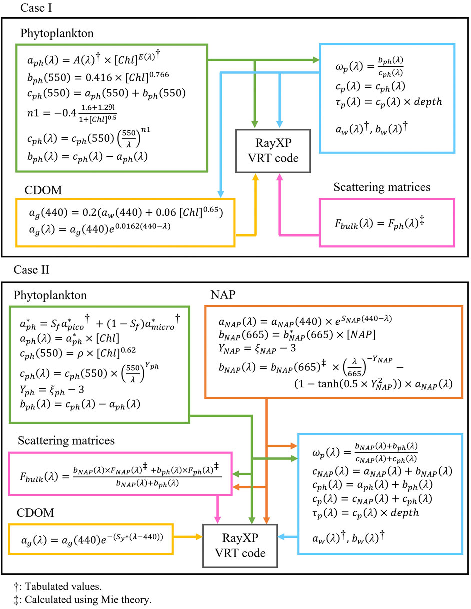
FIGURE 1. Flow diagram of the Case I and Case II bio-optical models.

TABLE 1

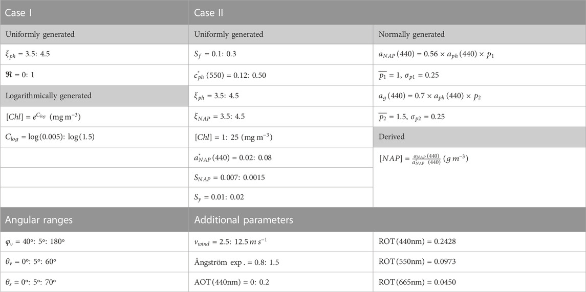
TABLE 1. Input generation ranges for the Case I and Case II bio-optical models of Figure 1 with additional atmospheric parameters and angular ranges used in the VRT calculations.

TABLE 2

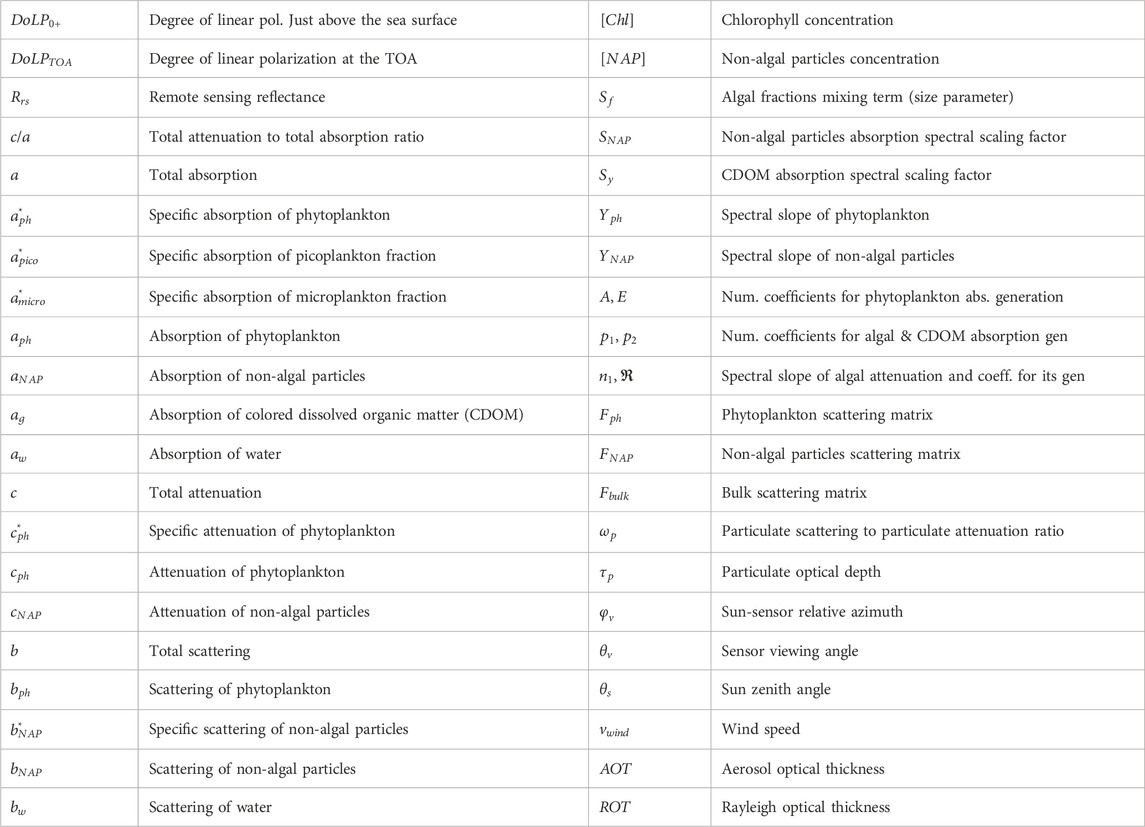
TABLE 2. List of symbols and acronyms for the bio-optical model parameters and neural network inputs and outputs.

2.3 VRT code

The calculations of polarized intensity values at the ocean surface level and at the TOA were carried out using the RayXP vector radiative transfer code (Zege et al., 1993; Tynes et al., 2001). The ocean-atmosphere system used in the code was modeled with four layers in total, three of them atmospheric and one oceanic, with a wind-roughened surface in between. The topmost atmospheric layer was defined to account for 64.74% of the total Rayleigh optical thickness (ROT), while the middle layer accounted for the entire aerosol optical thickness and for an additional 35% of the ROT. The above-surface location of the virtual sensor in the model was set between the middle and bottom layers in the atmosphere, with the latter accounting for the remaining 0.26% of the ROT. The single oceanic layer was set up to be optically deep to avoid any influence from the sea floor. Aerosol properties were defined in terms of aerosol optical thickness (AOT) and of Ångström exponent at 440 nm, and both were generated randomly from a uniform distribution focusing on small aerosol loadings, i.e., with AOT (440 nm) ranging between 0 and 0.2 (Table 1). Wind speed values were similarly generated randomly from a uniform distribution. The scattering matrices defining the optical properties of the aerosols were taken from the parameter library of the RayXP software. These consist in tabulated values for 20 wavelengths over the 337–3,500 nm range, with intermediate values retrieved through linear interpolation. In this study, we used the “oceanic” and “continental” settings, meant to simulate aerosols in a Case I and Case II scenario respectively. The “oceanic” setting is part of a set of simple aerosols based on the microphysical models given in Lenoble and Broquez (1984), and consists in particles with a mean radius of 0.458 µm and a real refractive index of ∼1.38 over our wavelengths of interest. For this aerosol type, single scattering albedo is fixed at 1 and extinction efficiency ranges from 2.34 to 2.44 between 440 and 665 nm. The “continental” setting is instead a mix of the other simple aerosol models, thus including several particle types with discrete mean radii and real refractive indices. For this aerosol type, single scattering albedo is ∼0.89 over our wavelengths of interest, with extinction efficiency ranging from 2.01 to 1.26 between 440 and 665 nm. The 3,000 sets of properties in the training sets were computed using aerosols with a “continental” setting for Case II, and with an “oceanic” setting for Case I. The 300 sets of properties in the testing sets were instead computed using aerosols with both “continental” and “oceanic” settings for both Case I and Case II, to test the impact on the results of an aerosol mix that deviates from training expectations. Rayleigh optical thickness values were set at typical levels for the wavelengths of interest in a marine context, and obtained from tabulated data (Bodhaine et al., 1999). With the scenario thus set up, the VRT code was then used to compute corresponding DoLP₀₊ and DoLP_TOA values over many different angular configurations of Sun and sensor. Angle ranges were 40°:180° in 5° increments for the relative azimuth (${\varphi }_v$), avoiding areas of direct Sun glint, 0°:60° in 5° increments for the sensor view zenith (${\theta }_v$) and 0°:70° in 5° increments for the Sun zenith (${\theta }_s$). In total, this produced 5,655 angular permutations, each with a corresponding DoLP value, for each individual set of oceanic and atmospheric properties in the training and testing sets (Table 1). Figure 2 shows two examples of these DoLP₀₊ and DoLP_TOA sets, one each for the Case I and Case II models. It should be noted that, although the relative azimuth range was restricted to avoid Sun glint, other undesirable contributions such as those from reflected skylight were kept as part of the DoLP calculations: this not only allows the possibility of future validation through direct comparison with ship-based polarimeter measurements, but is also in accordance with the goals of this study, i.e., trying to account for the propagation of light from the water through the interface and then through the atmosphere at multiple angles via neural networks without having to rely on the traditional correction methods used to isolate the DoLP of water-leaving radiance.

FIGURE 2

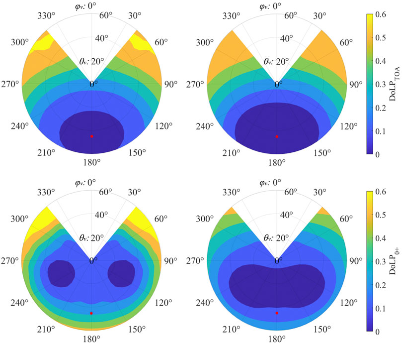
FIGURE 2. Polar contour plots of DoLP_TOA (top row) and DoLP₀₊ (bottom row) as calculated by the VRT code at 550 nm for two example sets of oceanic and atmospheric properties, one each for Case I (left column) and Case II (right column). Key input properties in the Case I example were: [Chl] = 0.05 mg m-3; Ångström exp. = 1.3; wind speed = 4.9 m/s; AOT (440) = 0.11. Key input properties in the Case II example were: [Chl] = 2.95 mg m-3; Ångström exp. = 1.04; wind speed = 3.2 m/s; AOT (440) = 0.11. The anti-solar point is marked in red.

2.4 ANN architectures

The 5,655 angular permutations considered within each VRT simulation in combination with the 3,000 individual sets of oceanic and atmospheric properties in the ANN training sets added up to a total of 16,965,000 distinct DoLP values. Similarly, the 300 sets of properties in the ANN testing sets added up to a total of 1,696,500 distinct DoLP values over all permutations. From among the several millions of DoLP values and corresponding properties in the training sets, 3,000,000 were randomly selected to function as validation during the development phase of the ANN training, i.e., as a subset against which to test during the training of the ANN. The validation frequency was set at 3 times per epoch, with a total of 12 epochs (the minibatch size was set as the square of the total number of input sets used for training). All selected input features were verified to be independent of each other (correlation score ∼0) and were standardized before training. The choice of features was informed by the results presented by Gao et al. (2021a); Gao et al. (2021b), suggesting that aerosol properties, wind speed and remote sensing reflectance will be available with good quality in the PACE data environment. However, in our study, remote sensing reflectance values were directly derived from the IOPs generated in the synthetic dataset using the following set of empirical relationships (Lee et al., 2002):

$u\left(\lambda \right)=b_b\left(\lambda \right)/\left(a\left(\lambda \right)+b_b\left(\lambda \right)\right)(1)$

$r_{rs}\left(\lambda \right)=0.125{\left[u\left(\lambda \right)\right]}^2+0.089u\left(\lambda \right)(2)$

$R_{rs}\left(\lambda \right)=0.52r_{rs}\left(\lambda \right)/\left[1-1.7r_{rs}\left(\lambda \right)\right](3)$

Figure 3 offers an overview of the spectral profiles of R_rs and c/a in both the Case I and Case II test sets. R_rs and c/a appear to be strongly correlated in both cases, but, crucially, feature an inversion of the spectral behavior of R_rs in Case I sets below ∼500 nm, as better captured by the direct comparison of R_rs vs. c/a in Figure 4. This suggests a possible guideline for the application of the Case I and Case II ANNs, whereby from around 0.0075 sr⁻¹ R_rs values at 440 nm tend to increase/decrease as particulate concentration and c/a decrease in Case I/Case II waters respectively. In both Case I and Case II ANNs, for the retrieval of DoLP₀₊ from DoLP_TOA specifically, we used the following inputs: R_rs and DoLP_TOA at 440, 550 and 665 nm, AOT (440), Ångström exponent, wind speed, solar zenith as well as sensor zenith and sun-relative azimuth. For the retrieval of the in-water c/a values from DoLP₀₊, we used the same inputs, but we substituted the three DoLP_TOA inputs with the corresponding three DoLP₀₊. Note that, since DoLP₀₊ is the output of the first ANN, work on the testing set was carried out by feeding the output of the first neural network directly into the second. We considered several ANN architectures (Table 3), with batch normalization and L2 regularization applied on all layers. Rectified linear units (ReLU) were used as activation functions on all hidden layers, while the Adam optimizer was used as the solver. The learning rate was set to an initial value of 0.01, with a rate drop factor of 0.1 every four epochs, and the root-mean-square error (RMSE) was used as the loss function on all architectures. The final architectures identified as the best ones after testing are highlighted in Table 3. Note that since the ANNs operate on all three wavelengths of interest simultaneously, the total number of inputs and outputs is 12 and 3 respectively for both DoLP₀₊ and c/a, reported as the first and last number of nodes in the architectures of Table 3.

FIGURE 3

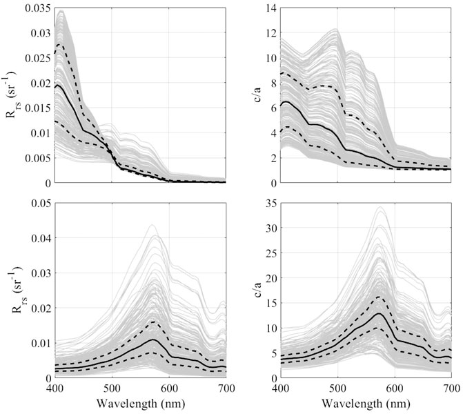
FIGURE 3. Spectral profiles of R_rs and c/a for the Case I (top row) and Case II (bottom row) test sets. Each grey line represents a single set of properties in the test set, with solid and dashed black lines representing overall median and quartiles respectively.

FIGURE 4

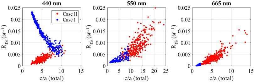
FIGURE 4. Distributions of c/a vs. R_rs values in the Case I and Case II test sets.

TABLE 3

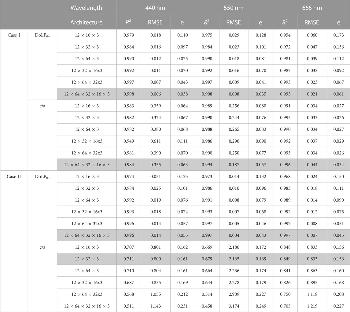
TABLE 3. Architectures of the ANNs tested for this study. The first and last number in each architecture describe inputs and outputs, with the remaining numbers describing the nodes in the hidden layers. Chosen architectures for each of the two ANNs in the Case I and Case II models are highlighted in grey. Scores are given for the baseline case with no uncertainties.

2.5 Uncertainties

To test the impact of uncertainties on the quality of the final c/a retrieval, we introduced random errors in the ANN inputs. The magnitude of the DoLP_TOA error was set to 1% following the stated mission target for PACE. The magnitude of the errors for AOT and wind speed was instead defined following Gao et al. (2021a), with the former set to $35.8e^{-3.824\times AOT\left(550\right)}$ (%) and the latter to $1.3\times AOT\left(550\right)+1.38$ m/s for wind speeds below 3 m/s and simply 1.2 m/s for wind speeds above 3 m/s. Finally, the magnitude of the errors for R_rs was set to 0.003, 0.002 and 0.001 sr⁻¹ respectively for 440, 550 and 665 nm following Gilerson et al. (2022). Note that AOT and wind speed errors are given as a function of AOT (550): in our case, AOT (550) was retrieved from the values of AOT (440) using the corresponding Ångström exponent values, and the empirical relationships themselves were extracted by exponential and linear fitting of the values presented in Figure 9 of the Gao et al. (2021a) paper for AOT and wind speed respectively. The numbers presented above are all used as an absolute scale: each was then paired and further scaled with a normally distributed random number $p_{\epsilon }$ ($\overline{x}=0,\sigma =1$), one for each corresponding feature within each set of values in the training and testing sets. AOT and DoLP_TOA errors are given as percentage, and were applied as

$x_i^{*}=x_i\hspace{0.17em}\ast \hspace{0.17em}\left(1+{\epsilon }_i\hspace{0.17em}\ast \hspace{0.17em}{p}_{\epsilon }\right)(4)$

with ${\epsilon }_i$ scaled as a number between 0 and 1, i.e., as the % value divided by 100. Here the subscript $i$ denotes either AOT or DoLP_TOA, $x_i^{*}$ is the value after application of the error, $x_i$ is the error-free value and ${\epsilon }_i$ is the error as indicated above. R_rs and wind speed are given in the corresponding absolute units and errors were therefore applied simply as

$x_i^{*}=x_i+{\epsilon }_i\hspace{0.17em}\ast \hspace{0.17em}{p}_{\epsilon }(5)$

where all symbols are the same as for Eq. 4 but the subscript $i$ denotes either R_rs or wind speed. In the following, the step-by-step uncertainty analysis will be illustrated using the Case II test set only. Although the exact statistical parameters will differ, the insights derived from the analysis apply to Case I as well. Case I and Case II will then be presented at the end in parallel with full uncertainties, i.e., with both uncertainties in the inputs and using an aerosol model that differs from the one used during training.

3 Results

3.1 Baseline case

A basic application of the DoLP neural network to the test data, that is with no consideration for uncertainty in the inputs and with continental-type aerosols consistent with the training data, produces results that are strongly consistent with expected values (Figure 5, top row). Statistics, in terms of R-squared values and RMSE, indicate a strong adherence to a 1:1 relationship, with very small values of e, defined as the ratio between RMSE and the mean of the DoLP values. In our analysis, we also included mean absolute error (MAE) and multiplicative bias, recommended by Seegers et al. (2018) as robust quantities for ocean color algorithm evaluation. MAE, indicative of the magnitude of the error relative to the measurand, is found to be ∼27% across all three wavelengths considered, which is large compared to appearances and to what R-squared and RMSE values suggest. The multiplicative bias, indicative of the average ratio between expected and projected values, similarly suggests that projected values are as low as ∼0.86 times the expected ones at 440 nm. However, both of these coefficients are found to be driven by the large density of data points that are close to zero. When the projected DoLP values at the surface are in turn fed into the c/a neural network, the resulting values are distributed along the x-axis, in a series of normal or quasi-normal distributions of projected values over each of the 300 expected c/a values (Figure 5, middle row). This is a direct consequence of having multiple permutations of input angles corresponding to only one true c/a value in the water. When viewed as a density plot, the data points are strongly clustered at the center of each distribution, which translates to very small error bars after averaging (Figure 5, bottom row). The average projected c/a values themselves are clustered along the 1:1 line, as indicated by the MAE and bias values. However, there is also substantial inherent variance to the c/a retrieval, with R-squared ∼0.71, ∼0.68 and ∼0.85 at 440, 550 and 665 nm respectively and e values three to four times larger than in the DoLP₀₊ retrieval across all three wavelengths.

FIGURE 5

FIGURE 5. Density plot of the results of the retrieval of Case II DoLP₀₊ by the first ANN with no uncertainties in the inputs (top row), density plot of the results of the retrieval of Case II c/a by the second ANN with no uncertainties in the inputs (middle row), and same results as the latter after averaging across all angle permutations for each set of properties (bottom row).

3.2 Error in the ANN inputs

To investigate the effect of uncertainties on the overall quality of the retrieval, we started by introducing randomized errors on the inputs as described in Section 2.5. As shown in Figure 6 (top row), the introduction of uncertainty in the inputs produces a significant spread in the retrieval of DoLP values at the surface, as reflected by the values of e and MAE in particular. Most data points are still retrieved close to the 1:1 line, as indicated by the consistently high R-squared values. At the same time changes in the bias are negligible and still driven by a large number of values near zero. When fed into the c/a neural network, the DoLP values at the surface produce interesting results, in the sense that, as with DoLP, the spread of the data points distribution increases, but the values of c/a after averaging over all angular permutations show little change from the no-uncertainty scenario, with the only difference an expected small increase in the width of the error bars. All statistical measures considered are seen to differ at most by 2% or less compared with the no-uncertainty scenario (Figure 6, bottom row), sometimes even improving on the baseline scores, highlighting how the changes induced by the error in the inputs are small enough to be superseded by the small amount of noise inherent to the ANN retrieval process.

FIGURE 6

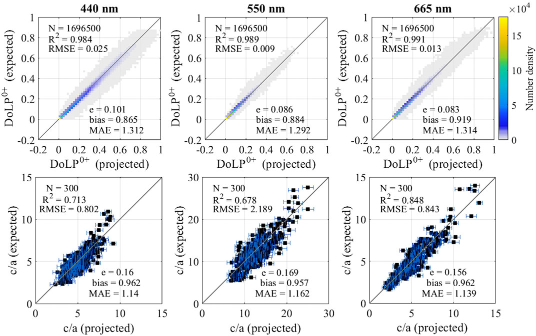
FIGURE 6. Density plot of the results of the retrieval of Case II DoLP₀₊ by the first ANN with errors applied to the inputs (top row), and results of the retrieval of Case II c/a by the second ANN with errors applied to the inputs after averaging across all angle permutations for each set of properties (bottom row).

3.3 Aerosol mix changes

As described in the Methods section, the neural networks for the Case II synthetic dataset were trained on data produced using an aerosol scattering model configured around a “continental” mix, selected to simulate coastal waters, proximal to an ideal landmass. Complementing the analysis done so far on similarly configured testing data, we produced a twin testing dataset reproducing the previous testing data in all respects save for the aerosol scattering model, which was instead set to “oceanic.” Feeding the resulting inputs into the neural network, we investigated the probable effects that an unexpected aerosol mix would have on the DoLP and c/a retrievals. The effect is seen to be small overall on the DoLP retrieval, with a larger variance at 550 nm and 665 nm. MAE is ∼6% higher at 440 nm, and ∼15% higher at 550 nm and 665 nm. Similarly, values of e are about 2 times and 4 times those of the baseline in the case of 440 nm and 550/665 nm respectively (Figure 7, top row). Overall, the effect is seen to be larger than that induced by uncertainties on the other ANN inputs. In contrast, the multiplicative bias, which was largely unchanged between the baseline and the input uncertainties case, is lower here, by ∼7%, ∼14% and ∼15% at 440 nm, 550 nm and 665 nm respectively. Similar to the input uncertainties case, there is little change from the baseline scenario in the c/a retrieval, with only slightly larger error bars. All statistical measures considered are seen to differ by at most ∼1% compared with the baseline scenario (Figure 7, bottom row).

FIGURE 7

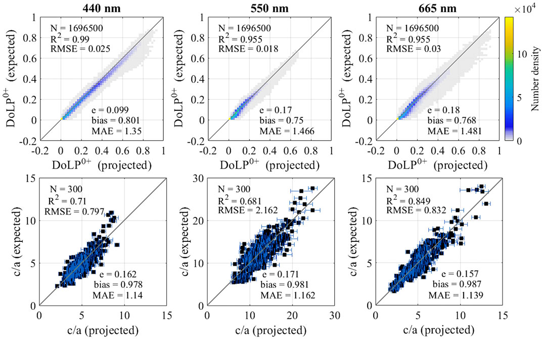
FIGURE 7. Density plot of the results of the retrieval of Case II DoLP₀₊ by the first ANN with aerosol mix changes (top row), and results of the retrieval of Case II c/a by the second ANN with aerosol mix changes after averaging across all angle permutations for each set of properties (bottom row).

3.4 Combined uncertainties

For the last comparison, input uncertainties and a non-standard aerosol mix were put together to examine their combined impact, now both in the Case I and Case II scenarios. As expected, deviations are largest compared with the baseline scenario. For Case II, the DoLP₀₊ retrieval presents bias values smaller by ∼7%, ∼13% and ∼14% and MAE values larger by ∼8%, ∼17% and ∼16% for 440 nm, 550 nm and 665 nm respectively (Figure 8, top row). RMSE and e values are both found to be ∼2.5 times and ∼4.5 times those of the baseline for 440 nm and 550/665 nm respectively. Nevertheless, changes in the average projected values in the c/a retrieval remained negligible, with all statistical measures found to differ at most by 2% or less compared with the baseline scenario (Figure 8, bottom row). For Case I, the DoLP₀₊ retrieval shows results similar to the Case II scenario, with statistical scores that are better across the board, particularly in terms of bias, with the sole exception of 665 nm, where an increased dispersion in the retrieved values induces a larger MAE score (Figure 9; top row). The most interesting differences are seen in the c/a retrieval for Case I, which is substantially more accurate than its Case II counterpart, with MAE values very close to 1 at all wavelengths (Figure 9, bottom row). In addition, where the c/a retrieval in Case II appeared roughly homoscedastic, i.e., with a variance that is about constant for increasing values of c/a, Case I appears instead heteroscedastic, i.e., the variance (as well as the width of the error bars) increases markedly as c/a values increase.

FIGURE 8

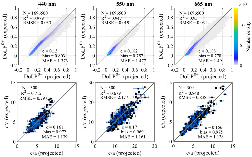
FIGURE 8. Density plot of the results of the retrieval of Case II DoLP₀₊ by the first ANN with combined uncertainties (top row), and results of the retrieval of Case II c/a by the second ANN with combined uncertainties after averaging across all angle permutations for each set of properties (bottom row).

FIGURE 9

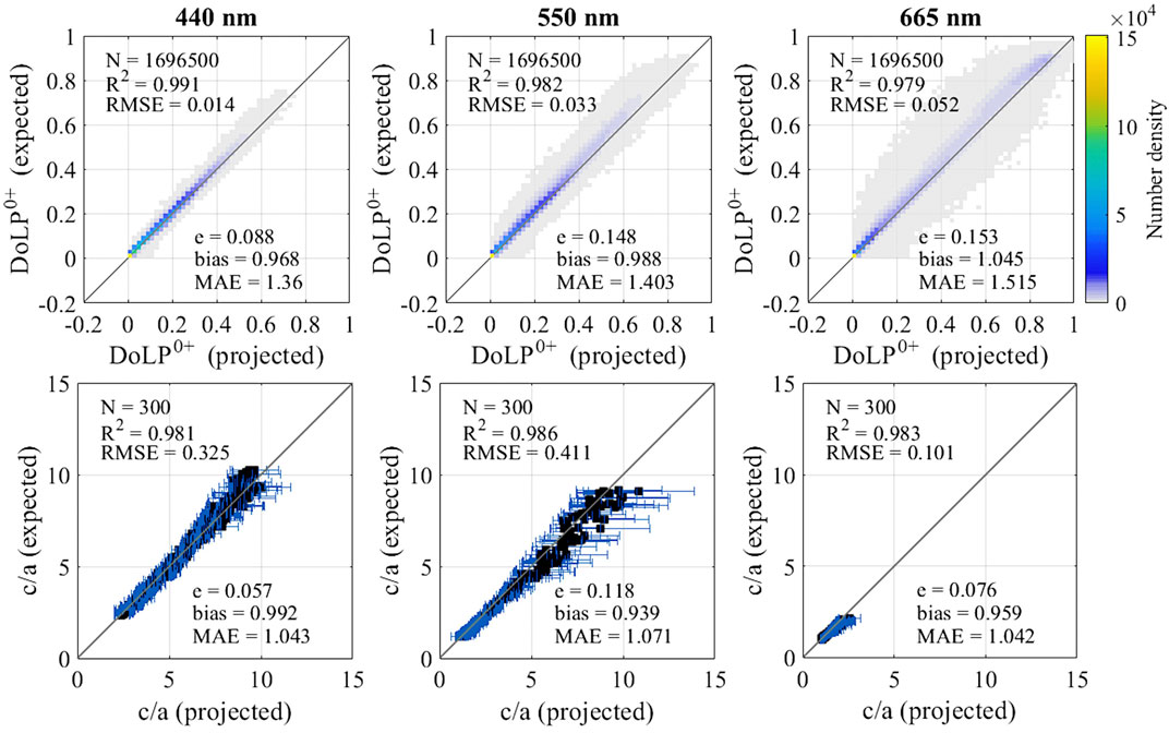
FIGURE 9. Density plot of the results of the retrieval of Case I DoLP₀₊ by the first ANN with combined uncertainties (top row), and results of the retrieval of Case I c/a by the second ANN with combined uncertainties after averaging across all angle permutations for each set of properties (bottom row).

4 Discussion

4.1 Synthetic dataset

The entirety of this work is predicated on the application of neural networks to synthetic datasets. While the construction of such datasets was made necessary by the lack of actual measurements in quantities large enough for training purposes, the fact remains that, at this point in time, no definitive judgment can be made on the quality of the DoLP₀₊ and c/a retrieval by the ANNs compared to real values as would be measured in situ by conventional methods. On the other hand, the datasets were constructed using a highly detailed bio-optical models, already used in the past with good results to investigate the relationship between polarization and IOPs in published literature (Figure 1; Tables 1, 2). The model was further paired with a state-of-the-art radiative transfer software for final calculations and a simulated atmosphere-ocean system with multiple layers defined along accepted standards. This study is therefore at least a valid exploration of the potential for ANNs to define a direct retrieval pipeline from PACE-like polarization data to surface layer IOPs in the ocean. To realize the full potential of the approach, two separate data strategies become apparent to deal with the two steps of the ANN retrieval. Pairs of DoLP_TOA and DoLP₀₊ measurements are expected to remain unavailable until the launch of the PACE mission itself, and as such this part of the algorithm will likely only be able to be developed against a real-world reference post factum. Pairs of DoLP₀₊ and surface layer IOP values can instead be retrieved right now, so that it is desirable to start building up a dataset as soon as possible. However, in both cases, having a solid synthetic dataset to work with will also be beneficial in the sense that it will enable transfer learning, i.e., an incremental refinement of the pre-trained networks by the addition of smaller amounts of new data. Consequently, while remarking the exploratory nature of this study, we expect the ANNs developed so far (and indeed any network developed along similar lines) to constitute a useful basis for the eventual development of newer iterations once real data becomes available in sufficient quantities. As it stands, our results suggest that an ANN approach to the direct estimation of surface layer IOPs from TOA polarization is a practical and useful tool for PACE applications that will work well in association with other algorithms developed to process PACE data.

4.2 Quality of the results

The quality of the c/a retrieval is found to be high even after the introduction of several uncertainties on the ANN inputs and the aerosol mix used in the radiative transfer calculations (Table 3; Figures 5–9), particularly for 440 nm and 665 nm. The intermediate step of DoLP₀₊ retrieval appears to be the most susceptible to the introduction of uncertainties, while c/a estimations after averaging appear to be consistently robust, with the most evident effect being a widening of the error bars around the mean values rather than a shift in the values themselves. This is due to the fact that additional variance in the retrieval of DoLP₀₊ translates to larger standard deviations but virtually unchanged means in the distribution of c/a values retrieved in the second ANN step. For reference, as reported in Section 3.3, for Case II the DoLP₀₊ retrieval in the combined uncertainties scenario deviates from the baseline with bias values smaller by 7%, 13% and 14% and MAE values larger by 8%, 17%, and 16% for 440nm, 550nm and 665 nm respectively (Figures 5–8). RMSE and e values are also both found to be ∼3.5 times and ∼4.5 times those of the baseline for 440nm and 550/665 nm respectively. Conversely, changes in the average projected values in the c/a retrieval are negligible, with all statistical measures found to differ at most by 2% or less compared with the baseline scenario. Comparatively, Case I retrieval is found to be even more accurate. For DoLP₀₊, bias scores are close to 1 across all three wavelengths of interest, with MAE values similarly improving on Case II scores with the sole exception of 665 nm. For c/a, the quality of the retrieval is particularly high, with both bias and MAE values close to 1 at all three wavelengths (Figure 9). As an additional detail, the variance of the Case I c/a retrieval appears to be markedly heteroscedastic, i.e., it increases as c/a increases, while the Case II c/a retrieval displays homoscedasticity, i.e., a somewhat constant variance across the range of c/a values. While on one hand the robustness of the c/a estimations is a desirable characteristic, on the other hand it seems to indicate that there are limited avenues for further improvement without a substantial reinterpretation of the approach. Indeed, at least in the Case II scenario, the error bars themselves, even in the combined uncertainties scenario, are small enough that deviations of the estimated c/a values from the 1:1 comparison with expected values cannot be ascribed to randomness, particularly at 550 nm where such deviations are found to be highest. The comparison instead highlights an inherent variance to the DoLP₀₊-c/a relationship that, for the moment, represents a ceiling to the quality of the retrieval reachable with the current iteration of our ANN approach. Furthermore, the robustness of the c/a retrieval across many hundreds of different angular combinations appears to contrast with previous findings that indicated the relationship between DoLP₀₊ and c/a values to be strongly affected by angular geometry (Ibrahim et al., 2016; Gilerson et al., 2020). Although no definitive explanation can be given at this time to reconcile this discrepancy, it appears likely that the higher dimensionality of the relationship as captured by the ANNs (12 inputs and 3 outputs over three separate wavelengths), with the explicit inclusion of R_rs values and opposed to the previous simple comparison of DoLP₀₊ vs. c/a at individual wavelengths, is sufficient for the networks to evaluate probable c/a values at most angles. Indeed it is worth noting that, while in principle some specific angles are optimal in terms of retrieval, i.e., ${\phi }_v=90°$ (Ibrahim et al., 2016; Gilerson et al., 2020), outside of glint-heavy directions such as ${\phi }_v\cong 180°$ near the antisolar point or ${\phi }_v\cong 0°$ most other angular combinations will still offer some predictive power even with a simple DoLP vs. c/a comparison (cf. Figure 8 in Ibrahim et al., 2016 for the below-water case), adding to the plausibility of higher dimensionality as a sufficient explanation for the performance of ANNs in this context.

4.3 HARP2 sampling

Studying the distribution of all possible angular permutations is both necessary in terms of ANN training and useful in terms of identifying what to expect in terms of the variance of the results. However, in actuality, the HARP2 instrument will scan its field of view across 10 view lines over the +-57° along-track range, each with a +-47° cross-track range. This means that, realistically, any given point on Earth’s surface will be imaged at most 10 times over a single transit, possibly less in case of cloud coverage or any other of the various quality flags. Therefore, it is important to consider how the practical concerns of sampling will affect the results seen so far. The statistical distributions considered so far already contain a large amount of information on what to expect. In the Case II scenario, the sets of projected c/a values produced for each set of oceanic and atmospheric properties across all angle permutations are distributed in a way that is found to be close to normal in all cases and at all wavelengths. Indeed, one in five is found to be strictly normal after testing for normality using the Shapiro-Wilk test at a p = 0.05 threshold (Shapiro and Wilk, 1965). In this situation, although the $N_{sample}$ polarization measurements (with $N_{sample}$ between 0 and 10) for any given point on the surface taken during a realistic PACE transit are not truly independent from each other (the various angular configurations being governed by orbital dynamics), on first approximation we may treat this problem in terms of the sample mean of a population, where the population in this case is the collection of all angular permutations and the samples are randomly selected from it. This is all the truer because the distribution of the sample mean will tend towards being normal even if the population distribution is not exactly normal, as indicated by the central limit theorem. Within this context, the standard error of the sample mean is

${\sigma }_{\mu }=\frac{{\sigma }_p}{\sqrt{N_{sample}}}(6)$

where ${\sigma }_p$ is the standard deviation of the population. Since the error bars described so far are themselves defined as ${\mu }_p\pm {\sigma }_p$, where ${\mu }_p$ is the population mean, we can readily reverse the problem and determine how likely it is for the mean of a sample of c/a values retrieved by the ANNs in a realistic scenario to fall within the $\pm {\sigma }_p$ error bars. Inverting Eq. 6 we simply obtain ${\sigma }_p=\sqrt{N_{sample}}\times {\sigma }_{\mu }$, and since ${\mu }_{\mu }={\mu }_p$ by definition (where ${\mu }_{\mu }$ is the mean of the sample mean distribution) and the probability that a normal deviate lies in the range between $\mu -k\sigma$ and $\mu +k\sigma$ is given by $\mathrm{erf}\left(k/\sqrt{2}\right)$, where erf is the error function, we find that on first approximation the mean of the c/a values retrieved from a set of realistically sampled measurements will fall within the error bars described so far in more than 90% of cases with as few measurements as $N_{sample}=3$. In the Case I scenario, the distributions of the sets of projected c/a values across all various angular permutations fail to test for normality in a vast majority of cases. While still having mean values close to the 1:1 optimum (Figure 9), they are instead found to feature long tails biased towards an overestimation of the expected c/a values. This violation of the assumptions used to validate the applicability of Eq. 6 to the Case II retrieval suggests that Case I is likely to be much more susceptible to small $N_{sample}$ values. To offer further confirmation of all this, it is possible to construct an astrodynamics model to simulate the orbit and attitude of PACE at any given time, allowing for the reconstruction of sets of realistic angles over which to experiment (Figure 10). To do so, we followed the closed-form geolocation algorithm presented by Patt and Gregg (1994), by which it is possible to obtain geodetic coordinates on the surface and the azimuth and zenith angles of both sensor and Sun for any sensor view orientation given the position and velocity of the parent satellite. Position and velocity were themselves obtained through the MATLAB Aerospace toolbox, with which we defined the PACE orbit using the intended parameters of 676.5 km altitude with a 98° inclination. The orbit was further characterized with a mean local time of the ascending node of 1 p.m., as per PACE specifications, and with an arbitrary starting date and time of 2024–06–01 at 8:59:23 UTC, resulting in a corresponding equation of time of 2.06 min and an apparent right Sun ascension of 4:39:15. Orbit ephemeris data were generated for a 2-days period following this arbitrary definition date. With these position and velocity tables defined, we randomly selected polling times for each set of properties in the testing set under the condition that, in cartesian coordinates, the resulting Z-component of the velocity was positive (i.e., the satellite was on the sunlit side of the orbit) and the resulting Z-component of the position was within ±4,200 km to avoid extreme angles at the poles. The position and velocities were then fed into the geolocation algorithm together with those of 240 neighboring orbital positions corresponding to a resolution of 5 s in a ±10 min window. The area thus defined was finally searched to identify the orbital positions by which each of the 10 HARP2 scan lines intersected the geodetic coordinates of the point directly at the nadir of PACE at the randomly selected polling time (Figure 10). The 10 positions were randomly reduced to $N_{sample}=3$, and the corresponding sensor view angles ${\theta }_v$, relative azimuth angles ${\varphi }_v$ and Sun zenith angles ${\theta }_s$ selected from the 5,655 pre-calculated combinations and fed together with the other corresponding properties in the testing set into the neural networks. Consistently with expectations, the results for Case II don’t majorly deviate from what was previously established in Figure 8, corroborating the implications of our statistical argument (Figure 11). Similarly, the Case I results do instead demonstrate a substantial increase in the variance of the c/a retrieval, confirming that, at least in our formulation, small $N_{sample}$ values are likely to adversely affect the quality of the Case I retrieval (Figure 12). Interestingly, and in contrast with the ensemble results of Figure 9, the comparison between projected and expected Case I c/a values appears to become homoscedastic, meaning that small $N_{sample}$ values may disproportionately affect low c/a values, while leaving the variance at high c/a values largely unchanged.

FIGURE 10

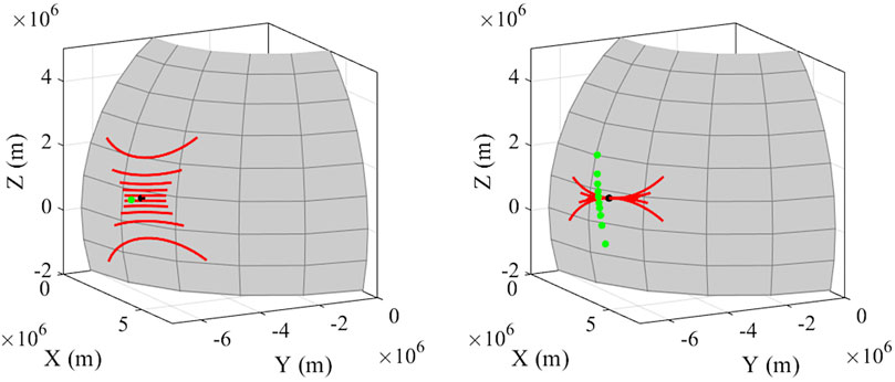
FIGURE 10. HARP2 scan configuration (red lines) for a given PACE orbital position (green circle) right above a given fixed point (black circle) on the surface of an Earth-sized sphere (left panel), and the ten PACE orbital positions for which the HARP2 scan lines overlap at the fixed point over a single transit (right panel).

FIGURE 11

FIGURE 11. Results of the retrieval of Case II DoLP₀₊ by the first ANN (top row), Case II c/a by the second ANN (middle row) and averages of the retrieved Case II c/a values (bottom row) after realistic sampling via simulation of the PACE orbit and of the HARP2 field of view for $N_{sample}=3$. Color groupings each pertain to an individual set of properties within the testing set.

FIGURE 12

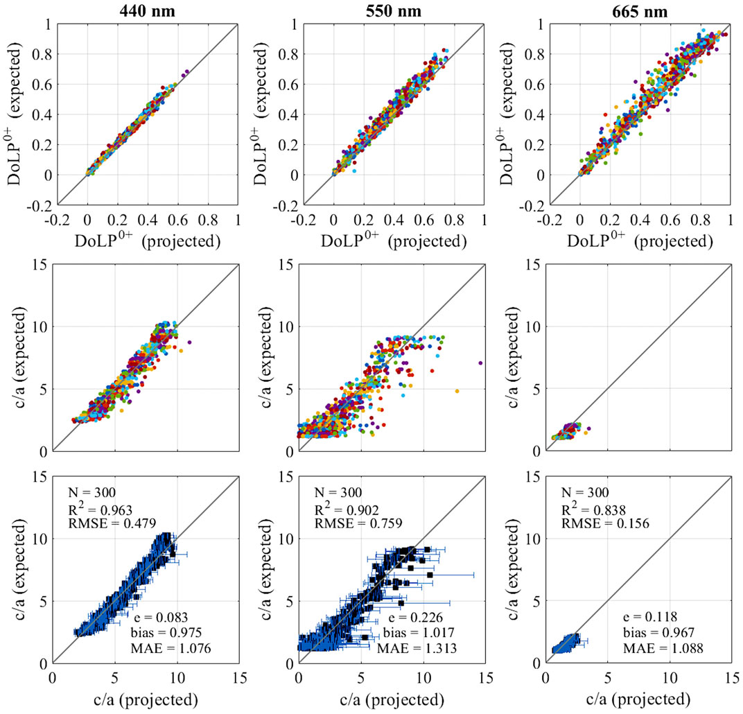
FIGURE 12. Results of the retrieval of Case I DoLP₀₊ by the first ANN (top row), Case I c/a by the second ANN (middle row) and averages of the retrieved Case I c/a values (bottom row) after realistic sampling via simulation of the PACE orbit and of the HARP2 field of view for $N_{sample}=3$. Color groupings each pertain to an individual set of properties within the testing set.

5 Conclusion

In this study we have explored the application of neural networks to the dual task of retrieving DoLP values at the ocean surface level from top-of-atmosphere DoLP values and in-water c/a values from DoLP values at the surface. The work was done within the context of the polarization measurements that are expected to be available once the upcoming PACE mission is launched, and the approach presented in this work uses input data that is expected be available within the PACE data environment. It is therefore designed to work well in tandem with other algorithms developed to process PACE polarization measurements. A scarcity of real-world data made the employment of synthetic datasets a necessity for the purpose of training our ANNs, so that no definitive judgement can be made on the quality of the ANN retrieval against real world data. Nevertheless, the specific characteristics of neural networks, including their capacity for adaptive re-training through transfer learning and the addition of new data, imply that the algorithms presented here will constitute a solid basis for quick iteration and further refinement once PACE data will become available. In the preliminary results presented in Agagliate et al. (2022), we identified a detailed analysis of the uncertainties in both the radiative transfer modeling and the ANN inputs as the path forward in the completion of our study. The introduction of uncertainties is found to have a large impact on the retrieval of DoLP₀₊ values, while the retrieval of c/a is found to be robust, with the largest effect observed in the overall size of the error bars but only minor changes in the mean c/a values. For both Case I and Case II, the quality of the c/a retrieval is high. For Case II, R² was equal to 0.712, 0.679, and 0.848 at 440, 550, and 665 nm respectively. Multiplicative bias is also small, underestimating expected values by only 2.8%, 3.1%, and 2.5% on average at those same wavelengths. Multiplicative MAE similarly indicates, on average, measurement errors of 13.9%, 16.1%, and 13.8% respectively. Case I results were even better, with R² equal to 0.981, 0.986, and 0.983 at 440, 550, and 665 nm respectively. Multiplicative bias was once again small, underestimating expected values by 0.8%, 6.1%, and 4.1% on average at the same wavelengths, while multiplicative MAE indicated measurement errors of only 4.3%, 7.1%, and 4.2% on average. The robustness of the c/a retrieval across many hundreds of different angular combinations appears to contradict earlier results that identified the DoLP₀₊-c/a relationship to be one particularly affected by the relative geometry of Sun and sensor (Ibrahim et al., 2016; Gilerson et al., 2020). It appears likely that the higher dimensionality of the relationship as captured by the neural networks (using 12 inputs over 3 wavelengths), specifically with the addition of R_rs, allows our algorithms to maintain discriminative power at all angle configurations. However, particularly for Case II, the general robustness of the approach is also found to imply that the inherent variance of the results in terms of the final retrieval of c/a values represents the current quality ceiling in the ability of our ANN to capture the relationship between the inputs and c/a, and may not be improved without a reinterpretation of the algorithm as a whole, e.g., with a radically different architecture or selection of the inputs. A final analysis step was carried out to examine the impact of realistic sampling on the expected results, i.e., with at most 10 measurements per transit per location, in contrast with the over 5,000 angular permutations considered during training. Due to the statistical distribution of the results, it is expected that averaging after sampling in such realistic conditions should, in a Case II scenario, follow closely the type of distribution presented in our study with as few as 3 measurements per location. Conversely, in a Case I scenario, this realistic averaging is instead expected to be susceptible to increased variance due to underlying distributions featuring long tails biased towards overestimation. Both expectations are found to be corroborated by results produced using an astrodynamics model that replicates the expected PACE orbit and the viewing area of the HARP2 instrument installed on it.

Data availability statement

The raw data supporting the conclusion of this article will be made available upon request by the authors, without undue reservation.

Author contributions

JA was responsible for simulations, data analysis and the bulk of the write up, as well as contributing to the general research direction of the study. RF and AI contributed considerable feedback, additions and corrections to the text. AG was the main contributor to the general research direction of the study, and additionally contributed feedback, suggestions and additions to the text.

Funding

Study carried out with the support of NASA grant 80NSSC21K0562, NOAA CESSRST grant NA16SEC4810008, and the JPSS Cal/Val program.

Acknowledgments

The authors would like to thank Frederick S. Patt, SAIC and the Ocean Ecology Laboratory at NASA Goddard Space Flight Center, for the useful discussions, suggestions and additional details that helped construct the astrodynamics model of the PACE orbit and HARP2 field of view. The authors further wish to thank the reviewers for their careful reading of the manuscript and for their helpful comments and suggestions.

Conflict of interest

The authors declare that the research was conducted in the absence of any commercial or financial relationships that could be construed as a potential conflict of interest.

Publisher’s note

All claims expressed in this article are solely those of the authors and do not necessarily represent those of their affiliated organizations, or those of the publisher, the editors and the reviewers. Any product that may be evaluated in this article, or claim that may be made by its manufacturer, is not guaranteed or endorsed by the publisher.

References

Agagliate, J., Malinowski, M., Herrera, E., and Gilerson, A. (2022). Polarimetric imaging of the ocean surface for satellite-based ocean color applications. Proc. SPIE 12112, 121120I. doi:10.1117/12.2622484

CrossRef Full Text | Google Scholar

Bodhaine, B. A., Wood, N. B., Dutton, E. G., and Slusser, J. R. (1999). On Rayleigh optical depth calculations. J. Atmos. Ocean. Technol. 16, 1854–1871.

CrossRef Full Text | Google Scholar

Bricaud, A., Morel, A., Babin, M., Allali, K., and Claustre, H. (1998). Variations of light absorption by suspended particles with chlorophyll a concentration in oceanic (case 1) waters: Analysis and implications for bio-optical models. J. Geophys. Res. 103 (C13), 31033–31044. doi:10.1029/98jc02712

CrossRef Full Text | Google Scholar

Cetinić, I., Perry, M. J., Briggs, N. T., Kallin, E., D'Asaro, E. A., and Lee, C. M. (2012). Particulate organic carbon and inherent optical properties during 2008 North Atlantic Bloom Experiment. J. Geophys. Res. 117, C06028. doi:10.1029/2011jc007771

CrossRef Full Text | Google Scholar

Chami, M., and Mckee, D. (2007). Determination of biogeochemical properties of marine particles using above water measurements of the degree of polarization at the Brewster angle. Opt. Express 15 (15), 9494–9509. doi:10.1364/oe.15.009494

PubMed Abstract | CrossRef Full Text | Google Scholar

Chami, M., and Platel, M. D. (2007). Sensitivity of the retrieval of the inherent optical properties of marine particles in coastal waters to the directional variations and the polarization of the reflectance. J. Geophys. Res.-Oceans 112 (C5), C05037. doi:10.1029/2006jc003758

CrossRef Full Text | Google Scholar

Chami, M., Santer, R., and Dilligeard, E. (2001). Radiative transfer model for the computation of radiance and polarization in an ocean-atmosphere system: Polarization properties of suspended matter for remote sensing. Appl. Opt. 40, 2398–2416. doi:10.1364/ao.40.002398

PubMed Abstract | CrossRef Full Text | Google Scholar

Chen, J., Quan, W., Cui, T., and Song, Q. (2015). Estimation of total suspended matter concentration from MODIS data using a neural network model in the China eastern coastal zone. Estuar. Coast. Shelf Sci. 155, 104–113. doi:10.1016/j.ecss.2015.01.018

CrossRef Full Text | Google Scholar

Chen, J., Quan, W., Cui, T., Song, Q., and Lin, C. (2014). Remote sensing of absorption and scattering coefficient using neural network model: Development, validation, and application. Remote Sens. Environ. 149, 213–226. doi:10.1016/j.rse.2014.04.013

CrossRef Full Text | Google Scholar

Chen, N., Li, W., Gatebe, C., Tanikawa, T., Hori, M., Shimada, R., et al. (2018). New neural network cloud mask algorithm based on radiative transfer simulations. Remote Sens. Environ. 219, 62–71. doi:10.1016/j.rse.2018.09.029

CrossRef Full Text | Google Scholar

Chowdhary, J., Cairns, B., Waquet, F., Knobelspiesse, K., Ottaviani, M., Redemann, J., et al. (2012). Sensitivity of multiangle, multispectral polarimetric remote sensing over open oceans to waterleaving radiance: Analyses of RSP data acquired during the MILAGRO campaign. Remote Sens. Environ. 118, 284–308. doi:10.1016/j.rse.2011.11.003

CrossRef Full Text | Google Scholar

Ciotti, A. M., Lewis, M. R., and Cullen, J. J. (2002). Assessment of the relationships between dominant cell size in natural phytoplankton communities and the spectral shape of the absorption coefficient. Limnol. Oceanogr. 47 (2), 404–417. doi:10.4319/lo.2002.47.2.0404

CrossRef Full Text | Google Scholar

Di Noia, A., Hasekamp, O. P., Wu, L., van Diedenhoven, B., Cairns, B., and Yorks, J. E. (2017). Combined neural network/Phillips–Tikhonov approach to aerosol retrievals over land from the NASA Research Scanning Polarimeter. Atmos. Meas. Tech. 10, 4235–4252. doi:10.5194/amt-10-4235-2017

CrossRef Full Text | Google Scholar

Doerffer, R., and Schiller, H. (2000). Neural network for retrieval of concentrations of water constituents with the possibility of detecting exceptional out of scope spectra. Proc. IGARSS 2000 IEEE 2000 Int. 2, 714–717.

Google Scholar

El-habashi, A., Ioannou, I., Tomlinson, M. C., Stumpf, R. P., and Ahmed, S. (2016). Satellite retrievals of karenia brevis harmful algal blooms in the west Florida shelf using neural networks and comparisons with other techniques. Remote Sens. 8, 377. doi:10.3390/rs8050377

CrossRef Full Text | Google Scholar

Fan, Y., Li, S., Han, X., and Stamnes, K. (2020). Machine learning algorithms for retrievals of aerosol and ocean color products from FY-3D MERSI-II instrument. J. Quant. Spectrosc. Radiat. Transf. 250, 107042. doi:10.1016/j.jqsrt.2020.107042

CrossRef Full Text | Google Scholar

Fan, Y., Li, W., Chen, N., Ahn, J. H., Park, Y. J., Kratzer, S., et al. (2021). OC-SMART: A machine learning based data analysis platform for satellite ocean color sensors. Remote Sens. Environ. 253, 112236. doi:10.1016/j.rse.2020.112236

CrossRef Full Text | Google Scholar

Foster, R., and Gilerson, A. (2016). Polarized transfer functions of the ocean surface for above-surface determination of the vector submarine light field. Appl. Opt. 55, 9476–9494. doi:10.1364/ao.55.009476

PubMed Abstract | CrossRef Full Text | Google Scholar

Foster, R., Gray, D. J., Koestner, D., El-habashi, A., and Bowles, J. (2022). Hydrosol scattering matrix inversion across a fresnel boundary. Front. Remote Sens. 2, 791048. doi:10.3389/frsen.2021.791048

CrossRef Full Text | Google Scholar

Fougnie, B., Frouin, R., Lecomte, R. P., and Deschamps, P. Y. (1999). Reduction of skylight reflection effects in the above-water measurement of diffuse marine reflectance. Appl. Opt. 38, 3844–3856. doi:10.1364/ao.38.003844

PubMed Abstract | CrossRef Full Text | Google Scholar

Gao, M., Franz, B. A., Knobelspiesse, K., Zhai, P.-W., Martins, V., Burton, S., et al. (2021). Efficient multiangle polarimetric inversion of aerosols and ocean color powered by a deep neural network forward model. Atmos. Meas. Tech. 14, 4083–4110. doi:10.5194/amt-14-4083-2021

CrossRef Full Text | Google Scholar

Gao, M., Knobelspiesse, K., Franz, B. A., Zhai, P.-W., Martins, V., Burton, S. P., et al. (2021). Adaptive data screening for multi-angle polarimetric aerosol and Ocean Color remote sensing accelerated by deep learning. Front. Remote Sens. 2. doi:10.3389/frsen.2021.757832

CrossRef Full Text | Google Scholar

Gilerson, A. A., Stepinski, J., Ibrahim, A. I., You, Y., Sullivan, J. M., Twardowski, M. S., et al. (2013). Benthic effects on the polarization of light in shallow waters. Appl. Opt. 52, 8685–8705. doi:10.1364/ao.52.008685

PubMed Abstract | CrossRef Full Text | Google Scholar

Gilerson, A., Carrizo, C., Foster, R., and Harmel, T. (2018). Variability of the reflectance coefficient of skylight from the ocean surface and its implications to Ocean Color. Opt. Express 26, 9615–9633. doi:10.1364/oe.26.009615

PubMed Abstract | CrossRef Full Text | Google Scholar

Gilerson, A., Carrizo, C., Ibrahim, A., Foster, R., Harmel, T., El-Habashi, A., et al. (2020). Hyperspectral polarimetric imaging of the water surface and retrieval of water optical parameters from multi-angular polarimetric data. Appl. Opt. 59, C8–C20. doi:10.1364/ao.59.0000c8

PubMed Abstract | CrossRef Full Text | Google Scholar

Gilerson, A., Herrera-Estrella, E., Foster, R., Agagliate, J., Hu, C., Ibrahim, A., et al. (2022). Determining the primary sources of uncertainty in retrieval of marine remote sensing reflectance from satellite Ocean Color sensors. Front. Remote Sens. 3, 857530. doi:10.3389/frsen.2022.857530

CrossRef Full Text | Google Scholar

Gleason, A. C. R., Voss, K. J., Gordon, H. R., Twardowski, M. S., and Berthon, J.-F. (2018). Measuring and modeling the polarized upwelling radiance distribution in clear and coastal waters. Appl. Sci. 8, 2683. doi:10.3390/app8122683

CrossRef Full Text | Google Scholar

Harmel, T., Gilerson, A., Tonizzo, A., Chowdhary, J., Weidemann, A., Arnone, R., et al. (2012). Polarization impacts on the water-leaving radiance retrieval from above-water radiometric measurements. Appl. Opt. 51, 8324–8340. doi:10.1364/ao.51.008324

PubMed Abstract | CrossRef Full Text | Google Scholar

Harmel, T. (2016). “Recent developments in the use of polarization for marine environment monitoring from space,” in Light scattering reviews. Editor A. A. Kokhanovsky (Berlin Germany: Springer), 41–84.

CrossRef Full Text | Google Scholar

Harmel, T., Tonizzo, A., Ibrahim, A., Gilerson, A., Chowdhary, J., and Ahmed, S. (2011). Measuring underwater polarization field from above-water hyperspectral instrumentation for water composition retrieval. Proc. SPIE 8175, 817509.

CrossRef Full Text | Google Scholar

Hieronymi, M., Müller, D., and Doerffer, R. (2017). The olci neural network swarm (ONNS): A bio-geo-optical algorithm for open ocean and coastal waters. Front. Mar. Sci. 4, 140. doi:10.3389/fmars.2017.00140

CrossRef Full Text | Google Scholar

Ibrahim, A., Gilerson, A., Chowdhary, J., and Ahmed, S. (2016). Retrieval of macro-and micro-physical properties of oceanic hydrosols from polarimetric observations. Remote Sens. Environ. 186, 548–566. doi:10.1016/j.rse.2016.09.004

CrossRef Full Text | Google Scholar

Ibrahim, A., Gilerson, A., Harmel, T., Tonizzo, A., Chowdhary, J., and Ahmed, S. (2012). The relationship between upwelling underwater polarization and attenuation/absorption ratio. Opt. Express 20, 25662–25680. doi:10.1364/oe.20.025662

PubMed Abstract | CrossRef Full Text | Google Scholar

Ioannou, I., Gilerson, A., Gross, B., Moshary, F., and Ahmed, S. (2013). Deriving ocean color products using neural networks. Remote Sens. Environ. 134, 78–91. doi:10.1016/j.rse.2013.02.015

CrossRef Full Text | Google Scholar

IOCCG. (2003). Ocean Color algorithm working Group – June 2003 IOCCG report. Available at: https://www.ioccg.org/groups/lee_data.pdf [Accessed September 15 2022].

Google Scholar

Jamet, C., Ibrahim, A., Ahmad, Z., Angelini, F., Babin, M., Behrenfeld, M. J., et al. (2019). Going beyond standard ocean color observations: Lidar and polarimetry. Front. Mar. Sci. 6, 251. doi:10.3389/fmars.2019.00251

CrossRef Full Text | Google Scholar

Knobelspiesse, K., Cairns, B., Redemann, J., Bergstrom, R. W., and Stohl, A. (2011). Simultaneous retrieval of aerosol and cloud properties during the MILAGRO field campaign. Atmos. Chem. Phys. 11, 6245–6263. doi:10.5194/acp-11-6245-2011

CrossRef Full Text | Google Scholar

Lee, Z. P., Carder, K. L., and Arnone, R. A. (2002). Deriving inherent optical properties from water color: A multiband quasi-analytical algorithm for optically deep waters. Appl. Opt. 41 (27), 5755–5772. doi:10.1364/ao.41.005755

PubMed Abstract | CrossRef Full Text | Google Scholar

Lenoble, J., and Broquez, C. (1984). A comparitive review of radiation aerosol models. Contrib. Atmos. Phys. 57, 1–20.

Google Scholar

Liu, H., Li, Q., Bai, Y., Yang, C., Wang, J., Zhou, Q., et al. (2021). Improving satellite retrieval of oceanic particulate organic carbon concentrations using machine learning methods. Remote Sens. Environ. 256, 112316. doi:10.1016/j.rse.2021.112316

CrossRef Full Text | Google Scholar

Loisel, H., Duforet, L., Dessailly, D., Chami, M., and Dubuisson, P. (2008). Investigation of the variations in the water leaving polarized reflectance from the POLDER satellite data over two biogeochemical contrasted oceanic areas. Opt. Express 16 (17), 12905–12918. doi:10.1364/oe.16.012905

PubMed Abstract | CrossRef Full Text | Google Scholar

Lotsberg, J. K., and Stamnes, J. J. (2010). Impact of particulate oceanic composition on the radiance and polarization of underwater and backscattered light. Opt. Express 18 (10), 10432–10445. doi:10.1364/oe.18.010432

PubMed Abstract | CrossRef Full Text | Google Scholar

Mishchenko, M. I., Cairns, B., Hansen, J. E., Travis, D. L., Burg, R., Kaufman, Y. J., et al. (2004). Monitoring of aerosol forcing of climate from space: Analysis of measurement requirements. J. Quant. Spectrosc. Radiat. Transf. 88 (1–3), 149–161. doi:10.1016/j.jqsrt.2004.03.030

CrossRef Full Text | Google Scholar

Mishchenko, M. I., and Travis, L. D. (1997). Satellite retrieval of aerosol properties over the ocean using polarization as well as intensity of reflected sunlight. J. Geophys. Res. Atmos. 102, 16989–17013. doi:10.1029/96jd02425

CrossRef Full Text | Google Scholar

Mobley, C. D. (2015). Polarized reflectance and transmittance properties of windblown sea surfaces. Appl. Opt. 54, 4828–4849. doi:10.1364/ao.54.004828

PubMed Abstract | CrossRef Full Text | Google Scholar

Morel, A., and Maritorena, S. (2001). Bio-optical properties of oceanic waters: A reappraisal. J. Geophys. Res. 106 (C4), 7163–7180. doi:10.1029/2000jc000319

CrossRef Full Text | Google Scholar

Morel, A. (1974). “Optical properties of pure water and pure sea water,” in Optical aspects of Oceanography. Editors N. G. Jerlov, and E. S. Nielsen (New York: Academic Press), 1–24.

Google Scholar

NASA PACE. (2022c). HARP2 polarimeter. Available at: https://pace.oceansciences.org/harp2.htm [Accessed September 22 2022].

Google Scholar

NASA PACE. (2022a). Home. Available at: https://pace.oceansciences.org/home.htm [Accessed September 22 2022].

Google Scholar

NASA PACE. (2022b). Mission science objectives. Available at: https://pace.oceansciences.org/mission_science.htm [Accessed September 22 2022].

Google Scholar

Ottaviani, M., Foster, R., Gilerson, A., Ibrahim, A., Carrizo, C., El-Habashi, A., et al. (2018). Airborne and shipborne polarimetric measurements over open ocean and coastal waters: Intercomparisons and implications for spaceborne observations. Remote Sens. Environ. 206, 375–390. doi:10.1016/j.rse.2017.12.015

PubMed Abstract | CrossRef Full Text | Google Scholar

Patt, F. S., and Gregg, W. W. (1994). Exact closed-form geolocation algorithm for Earth survey sensors. Int. J. Remote Sens. 15 (18), 3719–3734. doi:10.1080/01431169408954354

CrossRef Full Text | Google Scholar

Pope, R. M., and Fry, E. S. (1997). Absorption spectrum (380–700 nm) of pure water II Integrating cavity measurements. Appl. Opt. 36 (33), 8710–8723. doi:10.1364/ao.36.008710

PubMed Abstract | CrossRef Full Text | Google Scholar

Schiller, H., and Doerffer, R. (1999). Neural network for emulation of an inverse model operational derivation of Case II water properties from MERIS data. Int. J. Rem. Sens. 20, 1735–1746. doi:10.1080/014311699212443

CrossRef Full Text | Google Scholar

Seegers, B. N., Stumpf, R. P., Schaeffer, B. A., Loftin, K. A., and Werdell, P. J. (2018). Performance metrics for the assessment of satellite data products: An ocean color case study. Opt. Express 26, 7404–7422. doi:10.1364/oe.26.007404

PubMed Abstract | CrossRef Full Text | Google Scholar

Shapiro, S. S., and Wilk, M. B. (1965). An analysis of variance test for normality (complete samples). Biometrika 52 (3–4), 591–611. doi:10.2307/2333709

CrossRef Full Text | Google Scholar

Stamnes, K., Hamre, B., Stamnes, S., Chen, N., Fan, Y., Li, W., et al. (2018). Progress in forward-inverse modeling based on radiative transfer tools for coupled atmosphere-snow/ice-ocean systems: A review and description of the AccuRT model. Appl. Sci. 8, 2682. doi:10.3390/app8122682

CrossRef Full Text | Google Scholar

Stamnes, S., Fan, Y., Chen, N., Li, W., Tanikawa, T., Lin, Z., et al. (2018). Advantages of measuring the Q Stokes parameter in addition to the total radiance I in the detection of absorbing aerosols. Front. Earth Sci. 6, 1–11. doi:10.3389/feart.2018.00034

CrossRef Full Text | Google Scholar

Syariz, M. A., Lin, C.-H., Nguyen, M. V., Jaelani, L. M., and Blanco, A. C. (2020). WaterNet: A convolutional neural network for chlorophyll-a concentration retrieval. Remote Sens. 12, 1966. doi:10.3390/rs12121966

CrossRef Full Text | Google Scholar

Tanaka, A., Kishino, M., Doerffer, R., Schiller, H., Oishi, T., and Kubota, T. (2004). Development of a neural network algorithm for retrieving concentrations of chlorophyll, suspended matter and yellow substance from radiance data of the Ocean Color and temperature scanner. Oceanogr 60, 519–530. doi:10.1023/b:joce.0000038345.99050.c0

CrossRef Full Text | Google Scholar

Tonizzo, A., Gilerson, A., Harmel, T., Ibrahim, A., Chowdhary, J., Gross, B., et al. (2011). Estimating particle composition and size distribution from polarized water-leaving radiance. Appl. Opt. 50, 5047–5058. doi:10.1364/ao.50.005047

CrossRef Full Text | Google Scholar

Tonizzo, A., Zhou, J., Gilerson, A., Twardowski, M. S., Gray, D. J., Arnone, R. A., et al. (2009). Polarized light in coastal waters: Hyperspectral and multiangular analysis. Opt. Express 17, 5666–5683. doi:10.1364/oe.17.005666

PubMed Abstract | CrossRef Full Text | Google Scholar

Twardowski, M. S., Boss, E. S., Macdonald, J. B., Pegau, W. S., Barnard, A. H., and Zaneveld, J. R. V. (2001). A model for estimating bulk refractive index from the optical backscattering ratio and the implications for understanding particle composition in case I and case II waters. J. Geophys. Research-Oceans 106 (C7), 14129–14142. doi:10.1029/2000jc000404

CrossRef Full Text | Google Scholar

Tynes, H. H., Kattawar, G. W., Zege, E. P., Katsev, I. L., Prikhach, A. S., and Chaikovskaya, L. I. (2001). Monte Carlo and multicomponent approximation methods for vector radiative transfer by use of effective mueller matrix calculations. Appl. Opt. 40 (3), 400–412. doi:10.1364/ao.40.000400

PubMed Abstract | CrossRef Full Text | Google Scholar

van de Hulst, H. C. (1981). Light scattering by small particles. New York: Dover Publications.

Google Scholar

Voss, K. J., and Fry, E. S. (1984). Measurement of the Mueller matrix for ocean water. Appl. Opt. 23, 4427–4439. doi:10.1364/ao.23.004427

PubMed Abstract | CrossRef Full Text | Google Scholar

You, Y., Tonizzo, A., Gilerson, A., Cummings, M. E., Brady, P. J., Sullivan, J., et al. (2011). Measurements and simulations of polarization states of underwater light in clear oceanic waters. Appl. Opt. 50, 4873–4893. doi:10.1364/ao.50.004873

PubMed Abstract | CrossRef Full Text | Google Scholar

Zege, E. P., Katsev, L. L., and Polonsky, I. N. (1993). Multicomponent approach to light propagation in clouds and mists. Appl. Opt. 32 (15), 2803–2812. doi:10.1364/ao.32.002803

PubMed Abstract | CrossRef Full Text | Google Scholar

Zhang, X., He, S., Shabani, A., Zhai, P. W., and Du, K. (2017). Spectral sea surface reflectance of skylight. Opt. Express 25, A1–A13. doi:10.1364/oe.25.0000a1

PubMed Abstract | CrossRef Full Text | Google Scholar