Assessment of using spaceborne LiDAR to monitor the particulate backscatter coefficient on large, freshwater lakes: A test using CALIPSO on Lake Michigan

1 Introduction

The particulate backscatter coefficient, or b_bp (m⁻¹), is a central inherent optical property that gives important insight into ecological processes that happen in large bodies of water. Specifically, b_bp has been used as a proxy for particulate organic carbon in regions where inorganic material concentrations are low (Cetinić et al., 2012). Through this connection, on the global oceans b_bp has been used to quantify global carbon stocks (Loisel et al., 2001; Stramski et al., 2008; Behrenfeld et al., 2013; Martinez-Vicente et al., 2013), track the vertical migrations of ocean animals (Burt and Tortell, 2018; Behrenfeld et al., 2019), quantify primary production (Behrenfeld et al., 2005; Westberry et al., 2008; Schulien et al., 2017), and can be used to potentially monitor the overall health of water environments. Typically, b_bp has been sampled globally on the open oceans via two methods. First, by way of in situ collected measurements from ship (Concannon and Prentice, 2008; Dickey et al., 2011), aircraft (Hair et al., 2016; Churnside et al., 2017; Churnside and Marchbanks, 2019), and float surveys (Bittig et al., 2021). Second, by using ocean color data derived from optical imagery satellites such as the MODerate-resolution Imaging Spectroradiometer (MODIS), in which a gridded b_bp product is created (Mélin, 2011; Blondeau-Patissier et al., 2014). Both of these methods have paved the path of b_bp monitoring over the last 20 years.

While in situ sampling and passive sensors are able to provide b_bp, they are not without drawbacks. In situ measurements via ship and aircraft are costly and the network of ARGO floats is limited in its spatial coverage. Likewise, MODIS derived b_bp can only be collected in the daytime and can have errors associated in excess of 50% (Hostetler et al., 2018; Jamet et al., 2019). These drawbacks gave rise to a new era of b_bp collection: LiDAR based satellites (Hostetler et al., 2018; Bisson et al., 2021). The Cloud-Aerosol LiDAR and Infrared Pathfinder Satellite Observation (CALIPSO) satellite was launched in 2006 with the primary goal of measuring the properties of clouds and aerosols in Earth’s atmosphere using LiDAR (Winker et al., 2009; 2010). However, over the 15 years lifespan of the satellite, secondary uses were identified including its ability to obtain b_bp, which was first done a decade ago (Behrenfeld et al., 2013). Since then, numerous studies have been done using CALIPSO and other LiDAR based satellites as a way of collecting b_bp (Lu et al., 2014; 2016; 2020; Behrenfeld et al., 2016; 2019; Bisson et al., 2021).

Most studies which have obtained b_bp from CALISPO have done so on the global oceans, though there have been studies done on a more localized scale (Dionisi et al., 2020). To date however, none have been done in a large freshwater environment. This is likely due to the spatial resolution of CALISPO satellite tracks, which are spaced at $\approx 150$ km apart. On the global oceans this is an acceptable resolution for binning the data into 2° by 2° boxes, such as in Behrenfeld et al. (2019). However on study regions similar in size to the Great Lakes, this would be ineffective as one bin would span the entire basin of a lake. Another likely reason that CALIPSO has not been used to study large lakes is the need for high resolution (in both time and space) wind speed measurements, which play a large roll in the calculation of b_bp (Behrenfeld et al., 2013; Hu and Zhai, 2016).

Inland, freshwater lakes can also be optically complex (case 2, (Morel and Prieur, 1977) when compared to marine environments (case 1, (Palmer et al., 2015). This stems mainly from differences in concentrations of optically active constitutes (OAC) compared to sections of the global oceans (Morel and Prieur, 1977; Gons et al., 2008; Mouw et al., 2015). Likewise, the specific biological makeup of phytoplankton assemblages can differ substantially between freshwater and marine environments (Elser and Hassett, 1994). In addition, changes in the vertical distribution of particulate assemblages can vary substantially on freshwater lakes when compared to their marine equivalent (Scofield et al., 2020). These phenomenon present their own set of challenges and are unique to the freshwater remote sensing world.

Drawbacks aside, CALIPSO does make passes over some of the worlds largest freshwater lakes, specifically Lake Michigan in the United States. While it is impossible to map trends across the entire lake using CALIPSO, it is possible to map trends across individual, satellite flyover tracks. In the scope of Great Lakes ecosystem, b_bp is important to the monitoring of overall lake health. Decreases in b_bp over a 14 year period on Lakes Michigan and Huron have been tied to the effect of dreissenid mussels, phosphorus abatement, and climate change on the lakes (Yousef et al., 2017). In addition, b_bp has been monitored and used on the lakes as a metric to assess particulate assemblages and better regulate optical signal remote sensing. As the fishing industry on the Great Lakes is upwards of a $7 billion per year trade, being able to remotely sense/monitor the health of the ecosystem through b_bp would be extremely valuable (Roth et al., 2012).

Because of high resolution wind speed forecasting obtained from the National Oceanic and Atmospheric Administration (NOAA)’s Great Lakes Coastal Forecasting System (GLCFS) (NOAA, 2022), we are able to obtain b_bp from CALIPSO across the lake. Likewise, because of both NOAA cruises over the last decade and because of recent advances in using MODIS to obtain b_bp (Shuchman et al., 2013), we are able to compare the results obtained from CALIPSO to others sampled over similar time periods and locations. Here we show a method of obtaining LiDAR derived b_bp on large, freshwater lakes and the challenges associated with it. We then compare these results to both in situ values and results obtained through passive sensors. We close by speculating on the roll that LiDAR obtained b_bp can play in the future of Great Lakes remote sensing.

2 Materials and methods

2.1 CALISPO b_bp

Data used in deriving bbp from CALIPSO comes from NASA/CNES’s LiDAR Level 1B profile data, Version 4–10 product (Winker et al., 2009). For the majority of this assessment, we followed Behrenfeld et al. (2013), implementing changes that have come about over the last decade to improve the reliability of the results (Lu et al., 2013; 2014; 2021b; Bisson et al., 2021). A schematic of how b_bp is derived from CALIPSO is shown in Figure 1. For the scope of this analysis, b_bp refers to the backscatter sampled at 532 nm. At every point along the satellite track, the co-polarized and cross-polarized channel returns are extracted. A cross-talk correction between the two channels is implemented and the transient response from the surface is removed (Lu et al., 2014; 2021b). The corrected signal is then used to calculate a depolarization ratio (δ_t) between the two channels for the first three bins below the surface of the water. Following this, a series of filtering is done to eliminate signals that would result in a contaminated result. Implementation of this filtering is as follows, as was done in Dionisi et al. (2020):

FIGURE 1

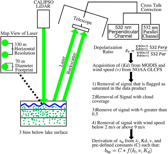
FIGURE 1. A schematic of how b_bp is obtained using the CALIPSO LiDAR. Briefly, the CALIPSO LiDAR profiles the water using two channels. A depolarization ratio (δ_t) is then calculated from the return, which is then further turned into b_bp following the method outlined in the text.

1) Removal of signal that is, flagged as saturated in the data product.

Lu et al. (2018) implemented a signal saturation flag to the CALIPSO data product. Here, we only consider data that is, not saturated in any way, and ignore data that is, flagged as possibly saturated or certainly saturated as this signal would not yield reliable results.

2) Removal of signal that had cloud coverage.

Clouds are identified though two sources. First, if the water surface peak from the LiDAR return is not within 120 m of the actual surface (derived from the Digital Elevation Model (DEM) flag on the CALIPSO data), then the signal is considered to be polluted by clouds. Second, if the integrated attenuated backscatter (IAB) for the entire LiDAR return is greater than a threshold value (0.017sr⁻1), then the signal is considered contaminated by clouds (Dionisi et al., 2020).

3) Removal of the signal where the depolarization ratio (δ_t) exceeded 0.5.

Realistic values of the depolarization ratio (δ_t) certainly would be below 0.5 (Dionisi et al., 2020). As such, all data returns with a depolarization ratio greater than 0.5 are not considered.

4) Removal of the signal where the wind speed is less than 2 m/s and greater than 9 m/s.

Low wind speeds (less than 2 m/s) result in signal saturation and high wind speeds (greater than 9 m/s) result in turbid waters. As each of these cases would result in an unreliable signal, they are therefore not considered.

After preliminary filtering of the signal, we were able to start the calculation of b_bp. This was done through the use of parameters taken from Behrenfeld et al. (2013), Bisson et al. (2021), and though two dynamic variables. A listing of the constants and values are shown in Table 1. The first dynamic variable used in deriving b_bp is the diffuse attenuation coefficient for downwelling irradiance (K_d), which is obtained from MODIS optical imagery. Specifics surrounding the acquisition of K_d are shown in Section 2.2. We chose to directly use the MODIS derived K_d measurements rather than using the empirical relationship for K_d in Bisson et al. (2021) because we are analyzing a freshwater environment. As such, the relationship between MODIS K_d and the depolarization ratio (δ_t) may be different. However, it is likely that using either method will result in a very similar result, as the K_d used in Bisson et al. (2021) is still derived from MODIS via an empirical relationship.

TABLE 1

TABLE 1. A listing of the constants used to derive b_bp from CALIPSO channel returns. Further information on the derivation can be found in Behrenfeld et al. (2013).

The second and most important dynamic variable in the derivation of b_bp from CALIPSO is water surface wind speed (v). Wind speed is used in deriving wave height (Cox and Munk, 1954; Hu et al., 2008), which is directly used in calculating b_bp from the depolarization ratio (δ_t). For every point along the CALIPSO tracks, we used a dynamic wind speed obtained from NOAA GLCFS (NOAA, 2022). The high temporal resolution of the wind speed model allowed us to have wind speed measurements down to the same hour of each CALIPSO flyover. High winds will result in waves that make the water too turbid to obtain reliable b_bp measurements and low wind speeds can result in signal saturation (Behrenfeld et al., 2013). As such, we implemented a filter by removing all measurements that had a wind speed greater than 9 m/s and less than 2 m/s (Dionisi et al., 2020), as is shown in the pre-processing steps. Thus, we can now define b_bp as a function of the depolarization ratio (δ_t), wind speed v), the attenuation coefficient for downwelling irradiance (K_d), and the combination of previously defined constants C) following the relationship shown in Behrenfeld et al. (2013) as:

$b_{bp}=C\ast f\left({\delta }_t,v,K_d\right)(1)$

2.2 MODIS b_bp and K_d

Level 2 MODIS imagery intersecting Lake Michigan was downloaded through the NASA Ocean Biology Processing Group (OBPG; https://oceancolor.gsfc.nasa.gov/). Each image was processed using the Color Producing Agents Algorithm (CPA-A; Shuchman et al. (2013)) in order to derive estimates of chlorophyll-a concentration, suspended minerals concentration, and CDOM (Colored Dissolved Organic Matter) absorption. Using these three estimates, bulk absorption and bulk backscatter coefficients were derived for the following MODIS bands: 412, 443, 488, 531, 547, and 667 nm. At the same bands, b_bp was computed from the bulk backscatter by removing the backscatter due to pure water (coefficients derived from Morel et al. (1974). The diffuse attenuation coefficient (K_d) at the above wavelengths was estimated using a method outlined in Lee et al. (2005), which uses the bulk absorption and backscatter coefficients as well as the solar zenith angle.

Yearly average images were also computed for both b_bp and K_d. First, daily average images were generated by computing the mean of overlapping pixels within all satellite images from a given day. The yearly average images were then computed as the mean of all daily images within that year.

2.3 In situ b_bp

In situ b_bp was sampled by the National Oceanic and Atmospheric Administration’s Great Lakes Environmental Research Laboratory (NOAA GLERL). This was done primarily in the spring (March-May) and summer (June-August), with a scattering of samples in the fall (September- November), at several stations on Lake Michigan between 2015 and 2019. Observations of b_bp were derived from data collected by a WET Labs BB9 sensor, which measures volume scattering coefficients at 9 wavelengths (412, 440, 488, 510, 532, 595, 650, 676, and 715 nm). During sampling, the BB9 is mounted in a package along with other sensors including a WET Labs ac-s, Sea-Bird CTD, and WET Labs fluorometer. Packaging these sensors provides concurrent measurements of salinity, temperature, and absorption which are necessary for processing BB9 data to b_bp. The package was deployed vertically through the water column using a crane.

Using the WAP software package (WET Labs), ac-s, CTD, and BB9 data were converted from binary data to text files, and BB9 data were processed to b_bp using protocols outlined in Zaneveld et al. (2003). First, the total volume scattering function (β_t) is corrected using the coincident total absorption (a_t) measurements from the ac-s after having been re-sampled to the BB9 wavelengths. Next, the volume scattering function of the water (β_w) was calculated according to Boss and Pegau (2001), utilizing the coincident CTD-measured temperature and salinity. The particulate fraction of the volume scattering function (β_p) is calculated as the difference between β_t and β_w. b_bp is then computed according to the following equation using a χ factor of 1.1 (Sullivan et al., 2013):

$b_{bp}=2\pi \ast \chi \ast {\beta }_p(2)$

Finally, the b_bp data is binned to 1 m with the vertical profiles then averaged between 0 and 50 m below the water surface.

2.4 Study regions

For the scope of this assessment, we chose to limit our study to only Lake Michigan rather than any of the other Great Lakes. This was done purposefully for a two main reasons. First, the way the CALISPO flyovers were oriented coincided very well with the geometry of the lake. For Lake Michigan, the satellite had two unbroken and intersecting day/night tracks that spanned a few degrees of latitude (Figure 2). This match up allowed us to effectively preform our analysis even with the limited spatial coverage of the CALISPO satellite. Secondly, the distribution of in situ sampled b_bp values was the highest in Lake Michigan. This distribution of samples along similar lines of latitude to that of the CALIPSO tracks allowed us to compare our derived product effectively. A map of both of the CALISPO tracks used in this survey along with the locations of all in situ sampling stations is shown in Figure 2.

FIGURE 2

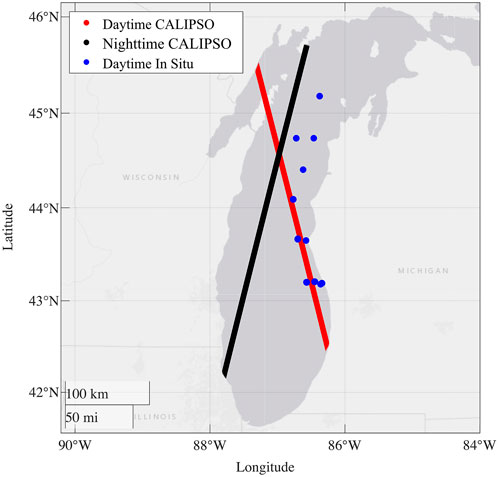
FIGURE 2. A map showing the location of the CALIPSO daytime (red), nighttime (black), and in situ (blue) measurement locations across Lake Michigan.

3 Results

3.1 Yearly average b_bp on Lake Michigan

As a first test of the ability to derive b_bp from CALIPSO, we computed an average b_bp across the entire lake for every year in the data record. We did this for both the daytime and nighttime CALIPSO tracks. To ascertain how this value compared to other measurements of b_bp, we took a yearly average b_bp for the MODIS data at the same location as the CALIPSO data. In conjunction with CALIPSO and MODIS, we also calculated a yearly average b_bp for the in situ data across the entire lake. We compared the three metrics in Figure 3A (daytime) and Figure 3B (nighttime). As MODIS is unable to sample at nighttime and as there is no documented nighttime b_bp samples on Lake Michigan, the nighttime b_bp from CALIPSO is compared to daytime measurements.

FIGURE 3

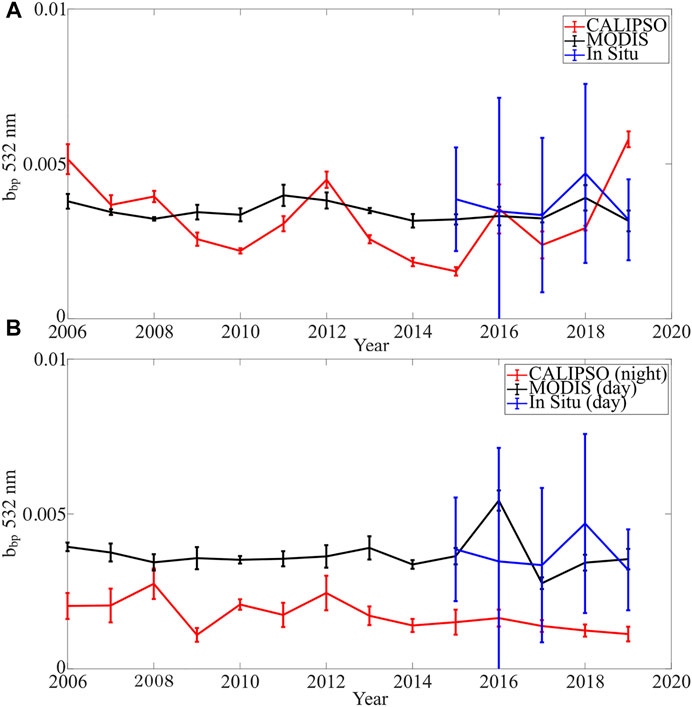
FIGURE 3. (A) Yearly b_bp daytime average across Lake Michigan for CALIPSO (red), MODIS (black), and in situ (blue). (B) Yearly b_bp nightime average across Lake Michigan for CALIPSO (red), MODIS (black), and in situ (blue). Here, MODIS and in situ values are still sampled in the daytime. Error bars for (A) and (B) represent 95% confidence. Intervals. Here, MODIS derived values are different across the lake because the daytime and nighttime CALIPSO tracks differ spatially.

Our results for the daytime flyovers showed more yearly variability in the CALIPSO b_bp than the MODIS b_bp (Figure 3A). However, over the course of the 15 year period, there was no discernible trend in b_bp (p-value $>0.05$). The 95% confidence bounds for the CALIPSO b_bp were similar to that of the MODIS derived results, and much smaller than the bounds on the in situ sampling. These results also held for the nighttime CALIPSO results (Figure 3B). However, the nighttime results are systematically lower for every year in the record when compared to their daytime counterparts and the MODIS/in situ data.

3.2 Seasonal b_bp across Lake Michigan

Both cloud cover and high wind speeds limited the return rate of usable CALIPSO data and therefore did not allow us resolve seasonal trends across the lake on a yearly basis. However, because trends across the 15 years time period of the CALIPSO, MODIS, and in situ data were largely unchanged (relative to the standard error of the in situ measurements), we felt justified in combining the entire time record into a seasonally divided data set and then evaluating this data set spatially across the lake. We did this for both the daytime and nighttime measurements. To start, the daytime measurements across Lake Michigan are shown in Figure 4A. These results are divided up into four seasons: Spring (March through May), Summer (June though August), Fall (September though November) and Winter (December through February).

FIGURE 4

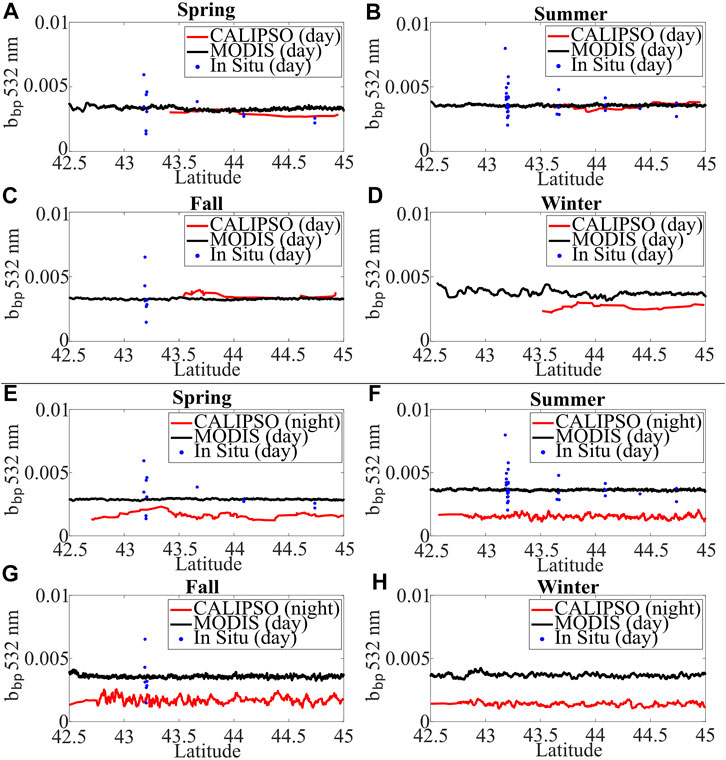
FIGURE 4. (A-D) Daytime, seasonal measurements for CALIPSO (red), MODIS (black), and in situ (blue) values of b_bp. (E-H) Nighttime, seasonal measurements for CALIPSO (red), MODIS (black), and in situ (blue) values of b_bp. Once again, MODIS and in situ values are still sampled in the daytime. Large variations in situ values can be partially attributed to differences in sampling longitude.

At a first order evaluation, for the spring, summer, and fall we see very good coherence between all three methods of collecting Daytime b_bp (Figure 4A). In the winter, we see a much larger divergence between measurements, which is not surprising in that the MODIS result is not well calibrated for winter. This could be related to one or more of the following potential issues. First, the CPA-A, which is used to generate the MODIS b_bp estimates, is calibrated based on in situ measurements throughout the lakes (Shuchman et al., 2013). However, because our in situ dataset does not include any measurements collected in winter, it is unclear how suitable the current calibration is during the winter season. Second, the CALIPSO result may also be influenced by ice in the lake. With these issues in mind, CALIPSO may be able to supplement non-existent winter sampling campaigns if validation of the result could be performed. The nighttime measurements from CALILPSO again show systematically lower response across all sections of the lake when compared to the daytime sampled results (Figure 4B). The usable data retrieval rate of the nighttime measurements was also nearly an order of magnitude higher then that of the daytime (7% vs. 1%).

Also of note is the lack of CALIPSO daytime data between 42.5° and 43.5°latitude. This likely is a direct result of the optical complexity of the waters of Lake Michigan in this region. Satellite optical imagery frequently shows the existence of sediment plumes in this part of the lake (Lohrenz et al., 2004; Vanderploeg et al., 2007), which may be resulting in a CALIPSO return that is, flagged as contaminated (for one or more of the previously shown filtering steps). Likewise, this part of the CALIPSO track is mostly nearshore, which further increases the optical complexity of the water and may result in further signal loss. This is also related to the large variability of in situ values in these optically complex waters, which are likely to have more variability in their b_bp relative to portions of the lake that are more spatially consistent.

3.3 Comparison of CALIPSO vs. MODIS daytime b_bp

To a higher level analysis of the daytime results, there is some smaller scale divergence across the lake between the CALIPSO and MODIS measurements. This is especially prevalent in the spring time (Figure 4A). Taking the in situ values as being ground truth, we next compared the daytime CALIPSO and MODIS b_bp results to the their closest measurement spatially on a seasonal basis, taking a median percent error for each season and instrument. We did this for both the spring and the summer separately (when in situ measurements were available) and then also combined the results across all seasons (Figure 5).

FIGURE 5

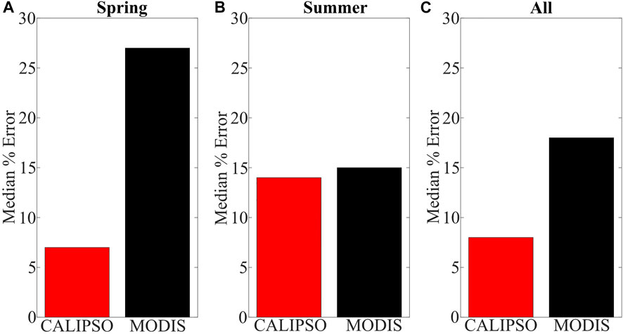
FIGURE 5. (A) Spring, (B) Summer and (C) Total percent error in CALISPO (red) and MODIS(black) for daytime measuremnts of b_bp.

We found that CALIPSO derived b_bp showed better agreement relative to the in situ sampling than the MODIS derived b_bp. This was especially true in the springtime where the CALIPSO b_bp had a median percent error of 7% and the MODIS b_bp had a median percent error of 27%. In the summer, both instruments were nearly the same in their performance, with the CALIPSO (14% error) only sightly outperforming the MODIS (15% error). Finally, taken together regardless of season, CALIPSO (8%) was closer to in situ values than MODIS (18%).

4 Discussion

4.1 Weather dependent return rate of CALIPSO

Our results indicate that CALIPSO can retrieve a reliable b_bp signal on a large, freshwater lake. However, deriving trends with a higher resolution than yearly across the entire lake or seasonally across the entire data record is impractical using the CALIPSO data. This is due to a weather dependent return rate of usable CALIPSO backscatter data across the lake. For daytime measurements, the amount of good measurements after filtering is around 1%. This improves substantially for the nighttime measurements where the amount of usable data climbs to approximately 7%. However, even at 7% retrieval, the limited spatially coverage of CALIPSO prevents a more in depth analysis.

Reasons for the low usable data percentage of CALIPSO on the Great Lakes stems mostly from two sources. First, average wind speeds on Lake Michigan are generally around 6 m/s, with values varying both spatially and temporally (Li et al., 2010). Due to turbid waters at high wind speeds and to signal saturation at low wind speeds, a range of wind speeds of between 2 m/s and 9 m/s is required in order to reliable derive b_bp from CALIPSO (Behrenfeld et al., 2013). Many of the CALIPSO flyovers on Lake Michigan take place when the wind speed is greater than the maximum allowed wind speed, resulting in a considerable loss of data. The second major source of data loss comes from the cloud coverage on the great lakes, where the percentage of cloud free days is less than 50% (Ju and Roy, 2008). Clouds prevent reliable retrieval of the signal from CALIPSO and therefor result in a null measurement.

A final note on the return rate of usable data from CALIPSO is the substantially higher retrieval rate in the nighttime hours to that of the daytime hours (7% vs. 1%). This is likely due to the behavior of clouds on wind speeds on Lake Michigan between the daytime and the nighttime. In the daytime, temperature gradients between the lake and the land produce high winds, an effect which may be diminished in the nighttime when temperature gradients are much less steep (Laird et al., 2001). This could result in both less cloud coverage and lower wind speeds on the lake in the evening hours, resulting in a higher data usability rate.

4.2 Substantial day/night difference in CALIPSO b_bp

As the usable data retrieval rate for nighttime measurements is higher for CALIPSO, it would be advantageous to use nighttime measurements of b_bp to further monitor the Great Lakes. However, our results indicate that there is a substantial offset in nighttime b_bp across all years (Figure 3B) and seasons (Figure 4B). This offset is sometimes more than 50% lower than the closest daytime measurement. Theory on the open ocean suggests that the nighttime measurement should be intrinsically 10% lower due to the diurnal size differences in particulates (Kheireddine and Antoine, 2014; Behrenfeld et al., 2019). This difference could be exacerbated in the freshwater ecosystem where zooplankton and phytoplankton are stoichiometricly distinct compared to their marine equivalent, and therefore could have much different and more amplified diurnal difference to their combined back-scattering (Elser and Hassett, 1994).

The challenge with validating the nighttime CALIPSO measurements is the lack of other sources of nighttime b_bp to compare it to. MODIS can only sample in the daytime as it is an optical instrument and there has not yet been any effort to sample b_bp in the nighttime across the Great Lakes. Because all current and future LiDAR based satellites will sample in the nighttime, and because the retrieval rate of usable data for nighttime measurements is nearly an order of magnitude better than daytime measurements, future sampling efforts across the Great Lakes should be gauged to have a nighttime component. This would serve to validate any future spaceborne LiDAR derived b_bp measurements.

4.3 CALIPSO b_bp as compared to MODIS b_bp

Our results indicated that daytime derived CALIPSO b_bp aligned better with the in situ sampling when compared to MODIS derived b_bp. This was especially true in the springtime where CALIPSO measurements were more than 20% closer to the in situ values than MODIS measurements. However, in the summer months CALIPSO was only slightly closer than MODIS, with a difference between them of less than 1%. This result is in line with previous studies on the global oceans, where CALIPSO performed better than MODIS when compared to in situ data gathered by the network of ARGO floats (Bisson et al., 2021). However, it should be noted that in situ sampling is quite variable and further analysis would be needed to further examine the performance of the CALIPSO measurements to MODIS measurements. For example, in situ measurements of b_bp on Lake Michigan are taken only periodically (usually twice a year) and only at one particular section of the lake. These sampling campaigns also are done via shipborne collection, which are intrinsically time consuming. To set up a more consistent and more efficient sampling campaign, it would be advantageous to establish a system of floats (similar to the open ocean) that could collect in situ values of b_bp regularly throughout the year. This would vastly improve the analysis.

The difference in reliability between the spring and summer for MODIS is likely due the summer biasing of the b_bp derivation from optical imagery. MODIS derivered b_bp is calculated, in part, by using in situ values to calibrate the method. Most of the in situ sampling that is, used to calibrate the MODIS derived product comes from summertime measurements. This results in a heavy biasing towards the summer months which yields a summertime MODIS b_bp that aligns better with in situ measurements and a springtime MODIS b_bp that diverges. Moreover, there is very little difference in coherence between seasons for CALIPSO because CALISPO derived b_bp is independent of in situ sampling campaigns.

4.4 The future of CALIPSO and LiDAR in large lake monitoring

Here, we derived b_bp from a spaceborne, LiDAR based, satellite on a large freshwater lake. We found that b_bp derived in this manner matches well with in situ sampled and MODIS derived b_bp values. We also found that the LiDAR derived values tend to be closer than the MODIS derived values when compared to the in situ values, however variability in the in situ sampling may be biasing this relationship. That said, the practicality of CALIPSO derived b_bp is limited on the Great Lakes due to three main reasons:

1) The weather dependent retrieval rate of daytime measurements is less than 1%, which makes monitoring small scale trends nearly impossible.

2) The spatial coverage of CALIPSO is limited in the scope of the Great Lakes, where the satellite only makes a few flyovers across repeat tracks.

3) CALIPSO, after 15 years in service, is nearing the end of its usable life and therefor further data that will be acquired by the satellite is likely minimal.

With these drawbacks in mind, the usability of CALIPSO derived b_bp on the Great Lakes likely lies in it ability to supplement in situ measurements, which are used to validate the gridded b_bp MODIS products. Previously, we stated that CALISPO was more in line with in situ measurements than MODIS, especially in the springtime. This is due to summer biasing which is related to the heavy summer distribution of in it situ measurements. However, CALIPSO derived results may be able to serve as proxy “in situ” b_bp values. This would greatly supplement current sampling efforts and improve MODIS derived b_bp products.

Even with CALISPO coming to an end, the future of spaceborne LiDAR derived b_bp on the Great Lakes is still bright. Recent studies on the global have used a new LiDAR based satellite that was launched in 2018, ICESat-2, to calculate b_bp both as an along track variable and as a function of water depth (Lu et al., 2020; 2021b; a). With considerably higher spatial coverage than CALIPSO and the ability to profile b_bp at depth, ICESat-2 could provide valuable information about water quality on the Great Lakes. With that in mind, we believe that spaceborne LiDAR will be a major component of monitoring efforts on the Great Lakes over the next 10 years.

Data availability statement

The raw data supporting the conclusions of this article will be made available by the authors, without undue reservation.

Author contributions

RW analyzed data and drafted the manuscript. MS and RS conceived the idea. KB processed the MODIS and in situ data. All authors contributed to the article and approved the submitted version.

Funding

This project was supported by the Great Lakes Restoration Initiative via interagency agreement DW-013-92543701 between EPA and NOAA. Funding was awarded to the Cooperative Institute for Great Lakes Research (CIGLR) through the NOAA Cooperative Agreement with the University of Michigan (NA17OAR4320152). This CIGLR contribution number is 1205.

Acknowledgments

The authors would like to thank the journal editor and reviewers. The authors would also like to thank NOAA and EPA for providing financial support. Specifically, we would like to thank Drs Hinchey and Tuchman from GLNPO and Ruberg and Vander Woude from NOAA/GLERL for encouraging this assessment.

Conflict of interest

The authors declare that the research was conducted in the absence of any commercial or financial relationships that could be construed as a potential conflict of interest.

Publisher’s note

All claims expressed in this article are solely those of the authors and do not necessarily represent those of their affiliated organizations, or those of the publisher, the editors and the reviewers. Any product that may be evaluated in this article, or claim that may be made by its manufacturer, is not guaranteed or endorsed by the publisher.

References

Behrenfeld, M. J., Boss, E., Siegel, D. A., and Shea, D. M. (2005). Carbon-based ocean productivity and phytoplankton physiology from space. Glob. Biogeochem. Cycles 19. doi:10.1029/2004gb002299

CrossRef Full Text | Google Scholar

Behrenfeld, M. J., Gaube, P., Penna, A. D., O’Malley, R. T., Burt, W. J., Hu, Y., et al. (2019). Global satellite-observed daily vertical migrations of ocean animals. Nature 576, 257–261. doi:10.1038/s41586-019-1796-9

PubMed Abstract | CrossRef Full Text | Google Scholar

Behrenfeld, M. J., Hu, Y., Hostetler, C. A., Dall’Olmo, G., Rodier, S. D., Hair, J. W., et al. (2013). Space-based lidar measurements of global ocean carbon stocks. Geophys. Res. Lett. 40, 4355–4360. doi:10.1002/grl.50816

CrossRef Full Text | Google Scholar

Behrenfeld, M. J., Hu, Y., O’Malley, R. T., Boss, E. S., Hostetler, C. A., Siegel, D. A., et al. (2016). Annual boom–bust cycles of polar phytoplankton biomass revealed by space-based lidar. Nat. Geosci. 10, 118–122. doi:10.1038/ngeo2861

CrossRef Full Text | Google Scholar

Bisson, K. M., Boss, E., Werdell, P. J., Ibrahim, A., and Behrenfeld, M. J. (2021). Particulate backscattering in the global ocean: A comparison of independent assessments. Geophys. Res. Lett. 48, e2020GL090909. doi:10.1029/2020gl090909

PubMed Abstract | CrossRef Full Text | Google Scholar

Bittig, H., Wong, A., and Plant, J. (2021). BGC-Argo synthetic profile file processing and format on Coriolis GDAC. Plouzané, France: Ifremer. doi:10.13155/55637

CrossRef Full Text | Google Scholar

Blondeau-Patissier, D., Gower, J. F., Dekker, A. G., Phinn, S. R., and Brando, V. E. (2014). A review of ocean color remote sensing methods and statistical techniques for the detection, mapping and analysis of phytoplankton blooms in coastal and open oceans. Prog. Oceanogr. 123, 123–144. doi:10.1016/j.pocean.2013.12.008

CrossRef Full Text | Google Scholar

Boss, E., and Pegau, W. S. (2001). Relationship of light scattering at an angle in the backward direction to the backscattering coefficient. Appl. Opt. 40, 5503–5507. doi:10.1364/ao.40.005503

PubMed Abstract | CrossRef Full Text | Google Scholar

Burt, W. J., and Tortell, P. D. (2018). Observations of zooplankton diel vertical migration from high-resolution surface ocean optical measurements. Geophys. Res. Lett. 45. doi:10.1029/2018gl079992

CrossRef Full Text | Google Scholar

Cetinić, I., Perry, M. J., Briggs, N. T., Kallin, E., D’Asaro, E. A., and Lee, C. M. (2012). Particulate organic carbon and inherent optical properties during 2008 north atlantic bloom experiment. J. Geophys. Res. Oceans 117. doi:10.1029/2011JC007771

CrossRef Full Text | Google Scholar

Churnside, J. H., and Marchbanks, R. D. (2019). Calibration of an airborne oceanographic lidar using ocean backscattering measurements from space. Opt. Express 27, A536. doi:10.1364/oe.27.00a536

PubMed Abstract | CrossRef Full Text | Google Scholar

Churnside, J., Marchbanks, R., Lembke, C., and Beckler, J. (2017). Optical backscattering measured by airborne lidar and underwater glider. Remote Sens. 9, 379. doi:10.3390/rs9040379

CrossRef Full Text | Google Scholar

Concannon, B. M., and Prentice, J. E. (2008). LOCO with a shipboard lidar. Tech. rep. Patuxent River, MD: NAVAL AIR SYSTEMS COMMAND PATUXENT RIVER MD.

Google Scholar

Cox, C., and Munk, W. (1954). Measurement of the roughness of the sea surface from photographs of the sun’s glitter. J. Opt. Soc. Am. 44, 838. doi:10.1364/josa.44.000838

CrossRef Full Text | Google Scholar

Dickey, T. D., Kattawar, G. W., and Voss, K. J. (2011). Shedding new light on light in the ocean. Phys. Today 64, 44–49. doi:10.1063/1.3580492

CrossRef Full Text | Google Scholar

Dionisi, D., Brando, V. E., Volpe, G., Colella, S., and Santoleri, R. (2020). Seasonal distributions of ocean particulate optical properties from spaceborne lidar measurements in mediterranean and black sea. Remote Sens. Environ. 247, 111889. doi:10.1016/j.rse.2020.111889

CrossRef Full Text | Google Scholar

Elser, J. J., and Hassett, R. P. (1994). A stoichiometric analysis of the zooplankton–phytoplankton interaction in marine and freshwater ecosystems. Nature 370, 211–213. doi:10.1038/370211a0

CrossRef Full Text | Google Scholar

Gilman, C., and Garrett, C. (1994). Heat flux parameterizations for the mediterranean sea: The role of atmospheric aerosols and constraints from the water budget. J. Geophys. Res. 99, 5119. doi:10.1029/93jc03069

CrossRef Full Text | Google Scholar

Gons, H. J., Auer, M. T., and Effler, S. W. (2008). MERIS satellite chlorophyll mapping of oligotrophic and eutrophic waters in the laurentian great lakes. Remote Sens. Environ. 112, 4098–4106. doi:10.1016/j.rse.2007.06.029

CrossRef Full Text | Google Scholar

Hair, J., Hostetler, C., Hu, Y., Behrenfeld, M., Butler, C., Harper, D., et al. (2016). Combined atmospheric and ocean profiling from an airborne high spectral resolution lidar. EPJ Web Conf. 119, 22001. doi:10.1051/epjconf/201611922001

CrossRef Full Text | Google Scholar

Hostetler, C. A., Behrenfeld, M. J., Hu, Y., Hair, J. W., and Schulien, J. A. (2018). Spaceborne lidar in the study of marine systems. Annu. Rev. Mar. Sci. 10, 121–147. doi:10.1146/annurev-marine-121916-063335

CrossRef Full Text | Google Scholar

Hu, Y., Stamnes, K., Vaughan, M., Pelon, J., Weimer, C., Wu, D., et al. (2008). Sea surface wind speed estimation from space-based lidar measurements. Atmos. Chem. Phys. 8, 3593–3601. doi:10.5194/acp-8-3593-2008

CrossRef Full Text | Google Scholar

Hu, Y., and Zhai, P. (2016). “Development and validation of the CALIPSO ocean subsurface data,” in 2016 IEEE international geoscience and remote sensing symposium (IGARSS) (IEEE). doi:10.1109/igarss.2016.7729981

CrossRef Full Text | Google Scholar

Jamet, C., Ibrahim, A., Ahmad, Z., Angelini, F., Babin, M., Behrenfeld, M. J., et al. (2019). Going beyond standard ocean color observations: Lidar and polarimetry. Front. Mar. Sci. 6. doi:10.3389/fmars.2019.00251

CrossRef Full Text | Google Scholar

Ju, J., and Roy, D. P. (2008). The availability of cloud-free Landsat ETM+ data over the conterminous United States and globally. Remote Sens. Environ. 112, 1196–1211. doi:10.1016/j.rse.2007.08.011

CrossRef Full Text | Google Scholar

Kheireddine, M., and Antoine, D. (2014). Diel variability of the beam attenuation and backscattering coefficients in the northwestern mediterranean sea (BOUSSOLE site). J. Geophys. Res. Oceans 119, 5465–5482. doi:10.1002/2014jc010007

CrossRef Full Text | Google Scholar

Kokhanovsky, A. A. (2003). Parameterization of the mueller matrix of oceanic waters. J. Geophys. Res. 108, 3175. doi:10.1029/2001jc001222

CrossRef Full Text | Google Scholar

Laird, N. F., Kristovich, D. A. R., Liang, X.-Z., Arritt, R. W., and Labas, K. (2001). Lake Michigan lake breezes: Climatology, local forcing, and synoptic environment. J. Appl. Meteorology 40, 409–424. doi:10.1175/1520-0450(2001)040⟨0409:lmlbcl⟩2.0.co;2

CrossRef Full Text | Google Scholar

Lee, Z.-P., Darecki, M., Carder, K. L., Davis, C. O., Stramski, D., and Rhea, W. J. (2005). Diffuse attenuation coefficient of downwelling irradiance: An evaluation of remote sensing methods. J. Geophys. Res. Oceans 110, C02017. doi:10.1029/2004jc002573

CrossRef Full Text | Google Scholar

Li, X., Zhong, S., Bian, X., and Heilman, W. E. (2010). Climate and climate variability of the wind power resources in the great lakes region of the United States. J. Geophys. Res. 115, D18107. doi:10.1029/2009jd013415

CrossRef Full Text | Google Scholar

Lohrenz, S. E., Fahnenstiel, G. L., Millie, D. F., Schofield, O. M. E., Johengen, T., and Bergmann, T. (2004). Spring phytoplankton photosynthesis, growth, and primary production and relationships to a recurrent coastal sediment plume and river inputs in southeastern lake Michigan. J. Geophys. Res. 109, C10S14. doi:10.1029/2004jc002383

CrossRef Full Text | Google Scholar

Loisel, H., Bosc, E., Stramski, D., Oubelkheir, K., and Deschamps, P.-Y. (2001). Seasonal variability of the backscattering coefficient in the mediterranean sea based on satellite SeaWiFS imagery. Geophys. Res. Lett. 28, 4203–4206. doi:10.1029/2001gl013863

CrossRef Full Text | Google Scholar

Lu, X., Hu, Y., Liu, Z., Zeng, S., and Trepte, C. (2013). “CALIOP receiver transient response study,” in SPIE proceedings. Editors J. A. Shaw,, and D. A. LeMaster (Bellingham, WA: SPIE). doi:10.1117/12.2033589

CrossRef Full Text | Google Scholar

Lu, X., Hu, Y., Pelon, J., Trepte, C., Liu, K., Rodier, S., et al. (2016). Retrieval of ocean subsurface particulate backscattering coefficient from space-borne CALIOP lidar measurements. Opt. Express 24, 29001. doi:10.1364/oe.24.029001

PubMed Abstract | CrossRef Full Text | Google Scholar

Lu, X., Hu, Y., Trepte, C., Zeng, S., and Churnside, J. H. (2014). Ocean subsurface studies with the CALIPSO spaceborne lidar. J. Geophys. Res. Oceans 119, 4305–4317. doi:10.1002/2014jc009970

CrossRef Full Text | Google Scholar

Lu, X., Hu, Y., Yang, Y., Bontempi, P., Omar, A., and Baize, R. (2020). Antarctic spring ice-edge blooms observed from space by ICESat-2. Remote Sens. Environ. 245, 111827. doi:10.1016/j.rse.2020.111827

CrossRef Full Text | Google Scholar

Lu, X., Hu, Y., Yang, Y., Neumann, T., Omar, A., Baize, R., et al. (2021a). New ocean subsurface optical properties from space lidars: CALIOP/CALIPSO and ATLAS/ICESat-2. Earth Space Sci. 8, e2021EA001729. doi:10.1029/2021EA001729

PubMed Abstract | CrossRef Full Text | Google Scholar

Lu, X., Hu, Y., Yang, Y., Vaughan, M., Liu, Z., Rodier, S., et al. (2018). Laser pulse bidirectional reflectance from CALIPSO mission. Atmos. Meas. Tech. 11, 3281–3296. doi:10.5194/amt-11-3281-2018

PubMed Abstract | CrossRef Full Text | Google Scholar

Lu, X., Hu, Y., Yang, Y., Vaughan, M., Palm, S., Trepte, C., et al. (2021b). Enabling value added scientific applications of ICESat-2 data with effective removal of afterpulses. Earth Space Sci. 8, e2021EA001729. doi:10.1029/2021ea001729

PubMed Abstract | CrossRef Full Text | Google Scholar

Martinez-Vicente, V., Dall’Olmo, G., Tarran, G., Boss, E., and Sathyendranath, S. (2013). Optical backscattering is correlated with phytoplankton carbon across the atlantic ocean. Geophys. Res. Lett. 40, 1154–1158. doi:10.1002/grl.50252

CrossRef Full Text | Google Scholar

Mélin, F. (2011). Comparison of SeaWiFS and MODIS time series of inherent optical properties for the adriatic sea. Ocean Sci. 7, 351–361. doi:10.5194/os-7-351-2011

CrossRef Full Text | Google Scholar

Morel, A. (1974). Optical properties of pure water and pure sea water.

Google Scholar

Morel, A., and Prieur, L. (1977). Analysis of variations in ocean color1. Limnol. Oceanogr. 22, 709–722. doi:10.4319/lo.1977.22.4.0709

CrossRef Full Text | Google Scholar

Mouw, C. B., Greb, S., Aurin, D., DiGiacomo, P. M., Lee, Z., Twardowski, M., et al. (2015). Aquatic color radiometry remote sensing of coastal and inland waters: Challenges and recommendations for future satellite missions. Remote Sens. Environ. 160, 15–30. doi:10.1016/j.rse.2015.02.001

CrossRef Full Text | Google Scholar

NOAA (2022). Noaa great lakes coastal forecasting system (glcfs). Ann Arbor, MI: lake michigan wind speed, 2006–2019.

Google Scholar

Palmer, S. C., Kutser, T., and Hunter, P. D. (2015). Remote sensing of inland waters: Challenges, progress and future directions. Remote Sens. Environ. 157, 1–8. doi:10.1016/j.rse.2014.09.021

CrossRef Full Text | Google Scholar

Roth, B., Mandrak, N., Hrabik, T., Sass, G., and Peters, J. (2012). Fishes and decapod crustaceans of the Great Lakes basin, 105–135.

Google Scholar

Schulien, J. A., Behrenfeld, M. J., Hair, J. W., Hostetler, C. A., and Twardowski, M. S. (2017). Vertically-resolved phytoplankton carbon and net primary production from a high spectral resolution lidar. Opt. Express 25, 13577. doi:10.1364/oe.25.013577

PubMed Abstract | CrossRef Full Text | Google Scholar

Scofield, A. E., Watkins, J. M., Osantowski, E., and Rudstam, L. G. (2020). Deep chlorophyll maxima across a trophic state gradient: A case study in the laurentian great lakes. Limnol. Oceanogr. 65, 2460–2484. doi:10.1002/lno.11464

PubMed Abstract | CrossRef Full Text | Google Scholar

Shuchman, R. A., Leshkevich, G., Sayers, M. J., Johengen, T. H., Brooks, C. N., and Pozdnyakov, D. (2013). An algorithm to retrieve chlorophyll, dissolved organic carbon, and suspended minerals from great lakes satellite data. J. Gt. Lakes. Res. 39, 14–33. doi:10.1016/j.jglr.2013.06.017

CrossRef Full Text | Google Scholar

Stramski, D., Reynolds, R. A., Babin, M., Kaczmarek, S., Lewis, M. R., Röttgers, R., et al. (2008). Relationships between the surface concentration of particulate organic carbon and optical properties in the eastern south Pacific and eastern atlantic oceans. Biogeosciences 5, 171–201. doi:10.5194/bg-5-171-2008

CrossRef Full Text | Google Scholar

Sullivan, J. M., Twardowski, M. S., Ronald, J., Zaneveld, V., and Moore, C. C. (2013). Measuring optical backscattering in water. Light Scatt. Rev. 7, 189–224.

CrossRef Full Text | Google Scholar

Vanderploeg, H. A., Johengen, T. H., Lavrentyev, P. J., Chen, C., Lang, G. A., Agy, M. A., et al. (2007). Anatomy of the recurrent coastal sediment plume in lake Michigan and its impacts on light climate, nutrients, and plankton. J. Geophys. Res. 112, C03S90. doi:10.1029/2004jc002379

CrossRef Full Text | Google Scholar

Voss, K. J., and Fry, E. S. (1984). Measurement of the mueller matrix for ocean water. Appl. Opt. 23, 4427. doi:10.1364/ao.23.004427

PubMed Abstract | CrossRef Full Text | Google Scholar

Westberry, T., Behrenfeld, M. J., Siegel, D. A., and Boss, E. (2008). Carbon-based primary productivity modeling with vertically resolved photoacclimation. Glob. Biogeochem. Cycles 22. doi:10.1029/2007gb003078.1029/2007gb003078

CrossRef Full Text | Google Scholar

Winker, D. M., Pelon, J., Coakley, J. A., Ackerman, S. A., Charlson, R. J., Colarco, P. R., et al. (2010). The CALIPSO mission. Bull. Am. Meteorological Soc. 91, 1211–1230. doi:10.1175/2010bams3009.1

CrossRef Full Text | Google Scholar

Winker, D. M., Vaughan, M. A., Omar, A., Hu, Y., Powell, K. A., Liu, Z., et al. (2009). Overview of the CALIPSO mission and CALIOP data processing algorithms. J. Atmos. Ocean. Technol. 26, 2310–2323. doi:10.1175/2009jtecha1281.1

CrossRef Full Text | Google Scholar

Yousef, F., Shuchman, R., Sayers, M., Fahnenstiel, G., and Henareh, A. (2017). Water clarity of the upper great lakes: Tracking changes between 1998–2012. J. Gt. Lakes. Res. 43, 239–247. doi:10.1016/j.jglr.2016.12.002

CrossRef Full Text | Google Scholar

Zaneveld, J. R. V., Pegau, S., and Mueller, J. L. (2003). Volume scattering function and backscattering coefficients: Instruments, characterization, field measurements, and data analysis protocols. Ocean Opt. Protoc. Satell. ocean color Sens. validation, Revis. 4, 65–76.

Google Scholar