Semi-analytical inversion modelling of Chlorophyll a variability in the U.S. Virgin Islands

1 Introduction

Coral reef communities are some of the most diverse and dynamic ecosystems on Earth. Warm-water coral reefs support hundreds of thousands of species that provide over 500 million people with food, income, and countless other ecosystem goods and services (Burke et al., 2011; Gattuso et al., 2014; Hoegh-Guldberg et al., 2017). Although they are an extremely valuable resources both ecologically and economically, the abundance of tropical coral reef ecosystems has declined over the past 30–50 years by at least 50% (Bruno and Selig, 2007; De’Ath et al., 2012; Hoegh-Guldberg, 2011; Hoegh-Guldberg et al., 2007; Hoegh-Guldberg et al., 2017; Hughes, 1994). These critical communities continue to decline at a rate of 1%–2% annually (Bruno and Selig, 2007). There are both global and local anthropogenic factors that contribute to this substantial decrease in coral reef ecosystem abundance.

The number of people visiting Caribbean islands has increased over the last 40 years in large part because of the scenic attributes of coral reefs and the clear waters and beaches that typically accompany them. To accommodate larger numbers of tourists, Caribbean Island nations are developing what was once natural vegetation at a rapid pace to build new roads, resorts, and other supporting infrastructure (Ramos-Scharrón and LaFevor, 2016). This development combined with the steep, mountainous hillsides typically found on many Caribbean islands is increasing erosion, sedimentation, and runoff beyond historic rates (Hubbard, 1987; Walling, 1997).

Terrestrial runoff is comprised of both organic and inorganic matter transported into the ocean when water from precipitation flows over the land surface. Runoff has the ability to significantly affect water quality by altering a water body’s normal biological, physical, and chemical characteristics. In particular, it can decrease light penetration and introduce excess nutrients, both of which can be detrimental to coral growth and health. As little as 10 mg cm^{2 −1} d⁻¹ of sediment deposition onto reefs can inhibit the growth of corals (Rogers, 1990) and sediment contact has been associated with coral disease (Brandt et al., 2013), and excess nutrients introduced by runoff can cause coastal eutrophication, stimulating benthic algal production, and facilitating shifts from coral to algal dominated substrates on reefs (Fabricius, 2005; Furnas et al., 2005; Weber et al., 2012). Benthic algae can inhibit corals by decreasing the amount of available sunlight and restricting growth and by outcompeting juvenile and adult corals for essential space (Bruno et al., 2003; Smith et al., 2006; Vega Thurber et al., 2014). Further, excess nutrients have been associated with increasing susceptibility to coral diseases (Bruno et al., 2003; Vega Thurber et al., 2014) and coral bleaching (Cunning and Baker, 2013), a breakdown in the symbiosis between the coral animal and its microalgal endosymbionts. In addition, eutrophication associated with runoff can also stimulate increasing abundance of phytoplankton, leading to increased concentrations of water column Chlorophylls, accessory pigments, and particulate organic matter, increasing turbidity levels (Furnas et al., 2005).

Indicators of water quality (e.g., Chlorophyll a) can be used to monitor the biophysical status of the waters as poor water quality is responsible for much of the coral reef degradation in the Caribbean (Edmunds and Gray, 2014; Gray et al., 2008; Gray et al., 2012; Smith et al., 2008). In addition, measures such as Chlorophyll a integrate inputs of excess nutrients into oligotrophic water better than direct nutrient monitoring, because tropical phytoplankton are primed for nutrient uptake and quickly scavenge all but the highest nutrient inputs (Furnas et al., 2005). This also means that dissolved nutrients in water samples do not reflect the actual inputs and are often near detection limits of analytical methods even with excess inputs. Conventional methods for assessing water quality are also based on in situ measurements that are both time consuming and costly. They lack the spatial and temporal coverage that can be achieved using alternative methods such as satellite based remote sensing.

Satellite remote sensing can monitor water bodies all over the world using models and algorithms calibrated to in situ measurements (McClain, 2009; Klemas, 2011; Ali et al., 2014). These models are used to monitor changes in aquatic environments in a timely manner over broad geographic regions. The spatial and spectral resolution of satellite remote sensing instruments (e.g., Landsat 8 OLI, Sentinel 2A/B MSI) has greatly improved in recent years leading to advancements in the quality of remote sensing products in coastal ecosystems.

NASA’s Ocean Biology Processing Group (OBPG) developed advanced optimization methods such as the Garver–Siegel–Maritorena (GSM) and Generalized Inherent Optical Properties (GIOP) to characterize the optical properties of water. This framework is built to facilitate applications of various semi-analytical (SAA) modeling approaches that are based on a quantitative description of absorption $\alpha \left(\lambda \right)$ and back scattering $b_b\left(\lambda \right),$ IOP properties of optically active constituents in water (Gordon et al., 1988). The GSM and GIOP models are used in this study because they have been shown to provide robust IOP estimates over a broad range of aquatic environments (Werdell et al., 2013; Clay et al., 2019; Werdell and McKinna, 2019; Lewis and Arrigo, 2020). These models differ in their basis vectors, spectral resolution, and parameterizations from each other.

The goal of the SAA inversion algorithms is to minimize the difference between modeled and observed $R_{rs}$ through empirical and optical closure relationships. Based on the radiative transfer definition and the optical closure functional relationship between $R_{rs}$ and IOPs (Gordon et al., 1988) defined the following:

${\mathit{R}}_{\mathit{r}\mathit{s}}\left(\mathit{\lambda }\right)=\mathit{f}.\mathit{u}(1)$

$u=\frac{b_b\left(\lambda \right)}{a\left(\lambda \right)+b_b\left(\lambda \right)}(2)$

where $f$ is a function that varies depending on boundary conditions such as the illumination conditions and volume scattering function. The IOP coefficients are partitioned into the additive components (Eqs 3, 4). Further each component is expressed as the product of its concentration specific absorption spectrum (eigenvector; a*) and its magnitude (eigenvalue, A and B):

$a\left(\lambda \right)=a_w\left(\lambda \right)+{\displaystyle {\sum }_{i=1}^{N_{ph}}}{A}_{p{h}_i}{a}_{p{h}_i}^{*}\left(\lambda \right)+{\displaystyle {\sum }_{i=1}^{N_d}}{A}_{d{g}_i}{a}_{d{g}_i}^{*}\left(\lambda \right)(3)$

and

$b_b\left(\lambda \right)=b_{bw}\left(\lambda \right)+{\displaystyle {\sum }_{i=1}^{N_{bp}}}{B}_{b{p}_i}{b}_{b{p}_i}^{*}\left(\lambda \right)(4)$

where the subscripts $w$, $ph$, $dg$ represent the absorption contributions from water, phytoplankton, non-algal particles (NAP) plus colored dissolved organic matter (CDOM), and the subscripts $bw$ and $bp$ represent the backscattering contributions from water and particulates, and the index I denote each IOP from 1 to N that are included in the model. Values of $a_w\left(\lambda \right)$ and $b_{bw}\left(\lambda \right)$ are known constants and provided by Pope and Fry (1997), and Smith and Baker (1981), respectively. The phytoplankton eigenvector, $a_{p{h}_i}^{*}\left(\lambda \right),$ varies by inversion model depending upon whether it will be used at global or regional scales. Global models typically use a more general phytoplankton absorption spectrum that can characterize many different phytoplankton functional types (Maritorena et al., 2002; Werdell et al., 2013). However, regional models use absorption spectra that are specific to the phytoplankton in that region (Roesler and Perry, 1995). The spectral shapes of NAP and CDOM absorption $\left.{\left(a\right.}_{d{g}_i}^{*}\left(\lambda \right)\right)$ are represented by exponential decay functions, and because they only differ in their exponential slopes, the two components are typically combined for remote sensing applications.

These are commonly expressed as:

$a_{dgi}^{*}\left(\lambda \right)={\exp }^{{\mathrm{S}}_{dg\left(\lambda -{\lambda }_0\right)}}(5)$

Where $S_{dg}$ typically vary between 0.01 and 0.02 nm⁻¹ (Gordon et al., 1988).

The eigenvector for particulate backscatter is typically represented by a power function:

$b_{b{p}_i}^{*}\left(\lambda \right)=\frac{{\mathrm{\lambda }}_0^{S_{bp}}}{\lambda }(6)$

where $S_{bp}$ defines the steepness of the power law as function of particle size.

Remote sensing reflectance and the eigenvector are used as the inputs for inversion models and the eigenvalues for absorption and backscattering ($A$ and $B$ from Eqs 3, 4) are estimated through optimization techniques (Roesler and Perry, 1995; Maritorena et al., 2002; Werdell et al., 2013).

$IOPs\left(\lambda \right)=f^{-1}\left[Rrs\left(\lambda \right)\right](7)$

IOP estimates ($A$ and $B$) can then be used to derive biogeochemical constituents such as Chlorophyll a (Chl-a) concentrations. Eigenvalues $B_{bphi}$ = $A_{p{h}_i}$, are concentrations of Chl-a.

In this study, the GSM and GIOP are applied to reflectance measurements to characterize the optical properties of the nearshore waters of the USVI. The calibrated model was then applied to Landsat 8 OLI sensor data to retrieve and map the spatial and temporal variability of the water quality using Chl-a as a primary index.

2 Study area

The U.S. Virgin Islands (USVI) are part of the Leeward Islands in the Lesser Antilles Island chain in the Caribbean which consists of three main islands: St. Thomas, St. John, and St. Croix as well as many islets, cays, and reefs (Figure 1). Oceanic water quality in this region is highly dependent upon weather, wave action, precipitation, and terrestrial development (Rothenberger et al., 2008). The average annual air temperatures of 28°C that varies slightly (5–10°C) throughout the year (Figure 2). The wet season runs from May to November and is generally dominated by Northeast trade winds in June and July (Schwartz, 2010). The rest of the year is typically drier with Southeast trade winds dominating from December to March (Schwartz, 2010). The average annual precipitation on St. Thomas and St. John ranges from 75–150 cm and is mostly due to the orthographic lifting of moist oceanic air over the hilly, mountainous terrain (Miller et al., 1997). However, the distribution of precipitation varies considerably within the USVI with the Western sides of the islands receiving much more rainfall than the Eastern sides. From May to November tropical low-pressure systems can form off the west coast of Africa and move westward across the Atlantic Ocean becoming tropical storms and hurricanes that can produce high winds and large amounts of precipitation for the USVI.

FIGURE 1

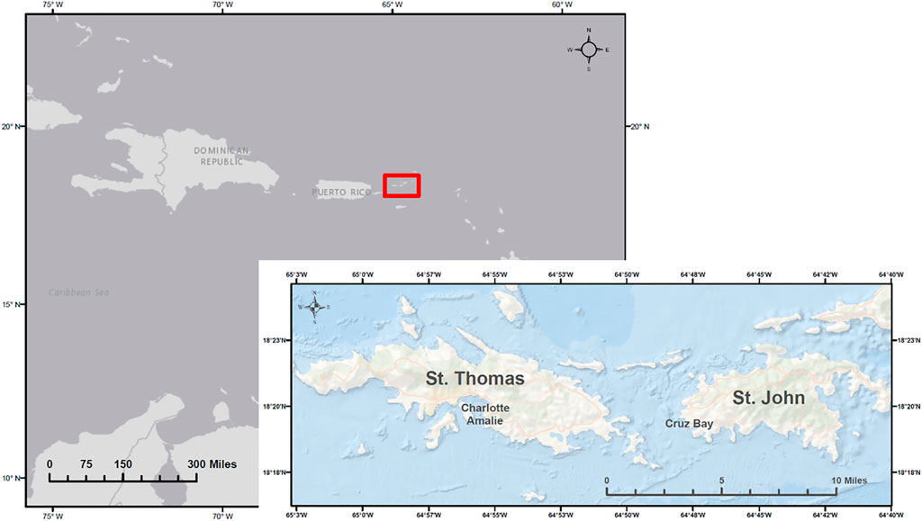
FIGURE 1. USVI is east of Puerto Rico in the Lesser Antilles Island chain, with an overview St. Thomas and St. John and the major towns on each island.

FIGURE 2

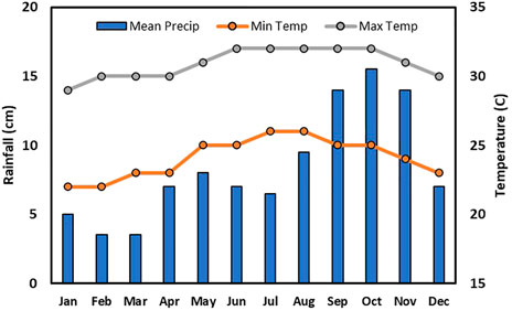
FIGURE 2. The seasonal variations in precipitation (cm) and temperature (˚C) in the USVI (NCDC, Cyril E. King Airport, St. Thomas, USVI).

3 Data and method

3.1 In-situ data

In-situ water quality and radiometric data were collected during four field campaigns: December 2016 June 2016, May-June 2017, and January 2018 at 17 sampling sites. Each campaign consisted of at least 7 sampling days and one or more corresponding satellite (Landsat 8 OLI) overpass days.

The sampling sites for this study are part of the USVI Territorial Coral Reef Monitoring Project (TCRMP) sites where coral reef health and benthic substrate metrics have been measured since 2001 (Table 1). All sites are located around the islands of St. Thomas and St. John in the Caribbean Sea. The sampling sites are also representative of different amounts of anthropogenic impact: low impact sites (FB, LB, Hind, SW, and NM) are either in deeper offshore waters removed from land-based influences or are associated with less disturbed or inhabited watersheds, medium impact sites (BP, Bot, BB, BI, FC, SV, SH, and SJ) are mid-shelf sites partially removed from land based sources of pollution or are onshore but receive from watersheds with moderate levels of development and high impact sites (H2, CR, CB, and MB) are associated with extensive harbor activities and/or high-density watershed development (Figure 3).

TABLE 1

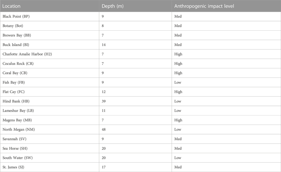
TABLE 1. Sampling sites and anthropogenic impact levels.

FIGURE 3

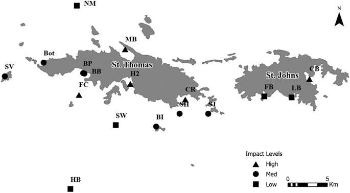
FIGURE 3. The locations of coral reef sites around St. Thomas and St. John where samples are collected during this study.

Water samples collected at each station were filtered using ashed, glass fiber filters (0.7 μm GF/F™), the Chl-a was extracted from each filter following EPA 445 method (Arar and Collins, 1997) and their concentration was measured fluorometrically using a calibrated bench top fluorometer. Chl-a fluorescence measurements were also measured in situ using Seabird CTD, WetLABS ECO meters. Two Satlantic hyperspectral radiometers (HyperOCR) integrated into a Wetlabs-ac-s optical package were used to collect down-welling irradiance (E_d (0-)) and upwelling radiance (L_u(0-)). The radiometers measure radiance between 350 and 800 nm at a 3.3 nm spectral interval and were resampled to spectral resolution of 10 nm. The data was pre-processed using instrument calibration files to eliminate noise (using tilt and velocity thresholds). The subsurface remote sensing reflectance $r_{rs}$ was obtained by:

$r_{rs}\left(\lambda ,0^{-}\right)=\frac{Lu\left(0-\right)}{Ed\left(0-\right)}(8)$

The ac-s profiler was also used to collect 159 IOPs measurements that were used to validate inversion models. The inversion of IOPs is a two-step process in which the IOPs are derived from the radiance and then biogeochemical parameters are derived from the IOPs.

3.2 Standard OC4 empirical algorithm

Satellite based sensors provide estimates of $R_{rs}\left(\lambda \right)$ after atmospheric correction is applied. The $R_{rs}\left(\lambda \right)$ is used to estimate the near-surface concentration of Chl-a based on empirical relationships. The OC4 is an empirical based blue-to-green band ratio algorithm that was initially adopted by NASA for SeaWiFS (O’Reilly et al., 1998; O’Reilly et al., 2000). It is based on a fourth-order polynomial regression between log-transformed Chl-a and log-transformed ratio of $R_{rs}\left(\lambda \right)$, as defined in Eq. 9:

$lo{g}_{10}\left(Chla\right)=a_0+{\displaystyle {\sum }_{i=1}^4}{a}_i{\left(lo{g}_{10}\left(\frac{\max \left(R_{rs}443;R_{rs}490;R_{rs}510\right)}{R_{rs}555}\right)\right)}^i(9)$

This algorithm is widely applied using current ocean color sensors (O’Reilly and Werdell, 2019).

3.3 Semi-analytical algorithms

Lee et al. (2002) developed an algorithm to convert $R_{rs}\left(\lambda \right)$ to their subsurface values for retrieving geophysical products:

$r_{rs}\left(\lambda ,0^{-}\right)=\frac{R_{rs}\left(\lambda \right)}{0.52+1.7R_{rs}\left(\lambda \right)}(10)$

Subsurface remote sensing reflectance ($r_{rs}\left(\lambda ,0^{-}\right)$) relates to IOPs by:

$r_{rs}\left(\lambda ,0^{-}\right)=G_1\left(\lambda \right)u\left(\lambda \right)+G_2\left(\lambda \right)u{\left(\lambda \right)}^2(11)$

where both $G_i\left(\lambda \right)$ vary with environmental parameters such as illumination, sea surface properties, and bidirectional effects. The $G_i\left(\lambda \right)$ values are estimated using several different methods such as in Gordon et al. (1988) where $G_1$ and $G_2$ are spectrally fixed (0.0949 and 0.0794, respectively). SAA models are then solved for $\mathrm{u}\left(\mathrm{\lambda }\right)$ (Eq. 11) by inverting $u\left(\mathrm{\lambda }\right)$ to estimate the eigenvalues for absorption and backscattering ($A$ and $B$ from Eqs 3, 4) using the Levenberg-Marquardt (LM) nonlinear optimization scheme. The LM optimization converges on a single eigenvalue or solution for $A$ and $B$. The eigenvalues are proportional to component concentration (Chl-a). The optimized eigenvalues ($A$ and $B$) are representative of the relative contributions of each absorbing and scattering spectral signature. The two SAA models employed here (GSM and GIOP) differ in their parametrization when modeling IOPs. GSM uses a constant value of 0.055 m²mg Chl-a⁻¹ for the Chl-a specific phytoplankton pigment absorption coefficient while GIOP uses $a_{ph}^{*}\left(\lambda \right)$ as a function of Chl-a concentrations (Bricaud et al., 1998). GIOP elements are therefore defined by specifying eigenvectors for each optically significant constituent assumed to exist in the regional water column (Werdell et al., 2013).

3.4 Satellite image processing

Level–1A Landsat 8 OLI images with less than 20% cloud cover were acquired from the USGS http://earthexplorer.usgs.gov/data gateway. To minimize the effects of temporal and spatial mismatches between the satellite and in situ data, only images that were within the time window ∼ ± 2 days of the Landsat–8 overpass was considered. The L2gen algorithm within SeaWiFS Data Analysis System scheme (SeaDAS version 7.5) was used to generate Level-2 geophysical products by applying the default atmospheric corrections and bio-optical algorithms to the Level-1A sensor data. The atmospheric correction was done by applying the default Near Infra-Red (NIR) technique (Gordon and Wang, 1994). The correction is based on the measured radiances at the two NIR wavelengths with the assumption that the water leaving radiances are negligible. IOP products were also retrieved for a_ph(l), at 412, 443, and 490 nm using the GIOP and GSM algorithm framework. To ensure spatial data consistency, Level-2 archive variable values were extracted from the images by running a 3 × 3 average kernel function surrounding the cloud-free sampling location.

3.5 Validation

Coefficient of determination, R² and the root mean square error (RMSE) were employed to assess model efficiency of IOP and Chl-a estimates. The IOP estimates were compared with in situ measurements from the WETLabs AC-S and the Chl-a estimates from the inversion models are compared with the laboratory-based Chl-a measurements.

4 Results

4.1 Meteorological conditions

4.1.1 Wind speed and direction

The meteorological conditions varied throughout the study period (Figure 4). Winds speeds ranged from 6–15 m/s and averaged approximately 10–11 m/s over all sampling dates. The summer 2016 and 2017 periods had the least variability in wind speed and averaged 11.3 m/s and 11.1 m/s, respectively. Sampling days in winter 2016 had an average wind of 10.0 m/s but ranged from 5.6–14.3 m/s. The summer 2016 study period had SE winds with the exception of 6/8/16 that had SSW winds. summer 2017 sampling days had very similar wind directions to the summer 2016 study period except for 5/20/2017, 5/21/2017, and 6/22/2017 that had more ENE winds. The wind direction during the winter 2016 sampling season was highly variable and ranged from NE on 12/8/2016 to SE on 12/10/2016.

FIGURE 4

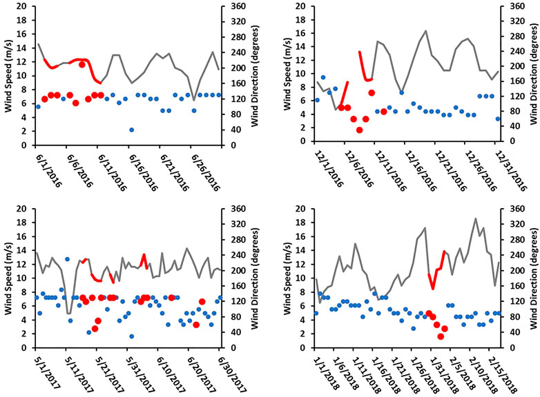
FIGURE 4. The daily wind speeds and directions for each month in which field sampling occurred. A solid grey line represents the wind speeds, and the wind directions are shown with blue circles. The particular wind speeds and directions during sampling days are highlighted in red (NCDC, Cyril E King Airport, St. Thomas, USVI).

4.1.2 Precipitation

Precipitation levels throughout the study periods were highly variable (Figure 5). The summer 2016 and 2017 sampling days had the highest rainfall totals with 3.9 and 5.0 cm, respectively. However, all 3.9 cm of rainfall in summer 2016 occurred in 1 day and was the single highest daily rainfall total measured. Only 1.2 cm of rainfall had occurred the entire month prior to sampling. The winter 2016 study period only had 1.1 cm of rainfall that coincides with the beginning of the annual dry season that runs from December to April. However, the previous month accumulated 18.9 cm of rain. Daily precipitation records during September and October of 2017 were unavailable due to Hurricanes Irma and Maria that hit the USVI on 9/6/17 and 9/25/17, respectively.

FIGURE 5

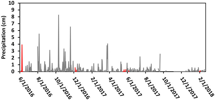
FIGURE 5. The daily precipitation (cm) recorded from June 2016 to February 2018. Sampling days are highlighted in red (NCDC, Cyril E King Airport, St. Thomas, USVI).

4.2 Chlorophyll a

Chlorophyll concentration is measured using the Seabird CTD, WetLABS ECO meter, aligned closely on the 1:1 line against the laboratory-based sample measurements, R² = 0.82 (Figure 6). The CTD Chl-a measurements had better agreement with laboratory measured concentrations (R² = 0.85) than the WetLABS ECO meter (R² = 0.80). The laboratory measured Chl-a concentrations ranged from 0.06 to 0.79 μg/L with an average value of 0.26 μg/L and a standard deviation (SD) of 0.16 μg/L. The lowest average Chl-a concentration was measured at the Hind Bank site (HB; 0.10 μg/L) with a standard error (SE) of 0.02 μg/L.

FIGURE 6

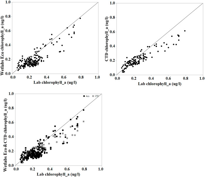
FIGURE 6. The correlation between Wetlabs Eco meter [Chl-a] (µg/L) (A), CTD [Chl-a] (µg/L) (B), and combined CTD and Wetlabs Eco meter [Chl-a] (µg/L) (C) with laboratory measured [Chl-a] (µg/L).

Sites located offshore of the mainland (HB, SW, BI, SH, SJ) and those in sparsely developed watersheds (Bot, FB, LB) show lower measures of Chl-a. Those sites within highly developed watersheds (MB, BP, BB, H2, CB) had the highest overall Chl-a concentrations. FC also appears as an outlier with higher amount of Chl-a in the winter season associated with rainfall. In general, the offshore sites had lower Chl-a concentrations than nearshore sites. (Figure 7).

FIGURE 7

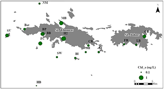
FIGURE 7. Average Chlorophyll a across sampling points.

Average Chl-a concentrations were greater in winter (Figure 8) and exhibited higher variability on a site by site and between site bases. summer 2016 and summer 2017 exhibited similar Chl-a concentrations, but there were some differences at select sites between the winter 2016–2017 and winter 2017–2018 Chl-a concentrations. The higher concentrations in winter 2016–2017 could be due to the 18.2 cm of rainfall that fell the month prior to samples collection.

FIGURE 8

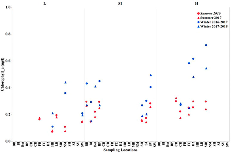
FIGURE 8. The seasonal average Chl-a concentration (µg/L) by impact levels (High, Medium and Low).

Chl-a concentrations also varied as a function of depth, particularly at nearshore sampling sites (Figure 9A). As distance from shore increased, there was less variation between individual daily measurements as well as Chl-a concentration with depth (Figures 9B, C). However, Chl-a profiles at HB in December 2016 showed increased concentration after approximately 30 m depth.

FIGURE 9

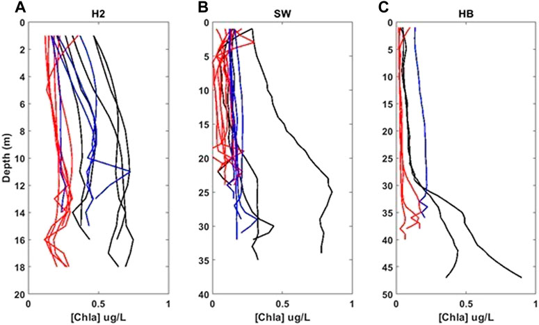
FIGURE 9. Chlorophyll a (µg/L) depth profiles for Charlotte Amalie Harbor (A), South Water (B), and Hind Bank (C) from all field campaigns: December 2016 (black), May/June 2017 (red), and January/February 2018 (blue). Note the change in depth scale from the onshore (H2) to the offshore (HB) site.

4.3 Model application

The accuracy of the three Chl-a algorithms was evaluated by computing the regression indices and statistical indicators summarized in Table 2.

TABLE 2

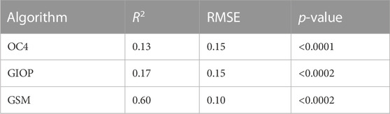
TABLE 2. Regression indices and statistical indicators for the Chl-a estimation in the USVI.

4.3.1 OC4 model

The global, OC4 algorithm exhibited the worst performance among the models, as evidenced by the low R² value (0.13) and relatively higher RMSE. The model consistently overestimates the Chl-a concentrations with bias of 0.2 μg/L.

4.3.2 GSM model

The GSM inversion model (Maritorena et al., 2002) was applied to 159 Satlantic HyperOCR R_rs measurements and the model results were compared with in situ total absorption, particulate backscatter, and Chl-a concentrations (Figure 10). The modeled a_t (443) ranged from 0.014 to 0.22 m⁻¹ with a mean of 0.077 m⁻¹ and a SE of 0.003 m⁻¹. Sites H2, CR and MB had the highest average $a_{tot}\left(443\right)$ of 0.125, 0.122 and 0.108 m⁻¹ with a SE of 0.008, 0.006 and 0.0278 m⁻¹ respectively. This was consistent with in situ a_tot measurements as well as the visually observed conditions during sampling. The H2 site was consistently visually turbid. CR and MB sites are shallow and were generally relatively more turbid than other sites. The lowest $a_{tot}\left(443\right)$ estimates were at offshore sites HB and NM with mean $a_{tot}\left(443\right)$ of 0.033 and 0.045 m⁻¹ with SE of 0.003 and 0.009 m⁻¹, respectively.

FIGURE 10

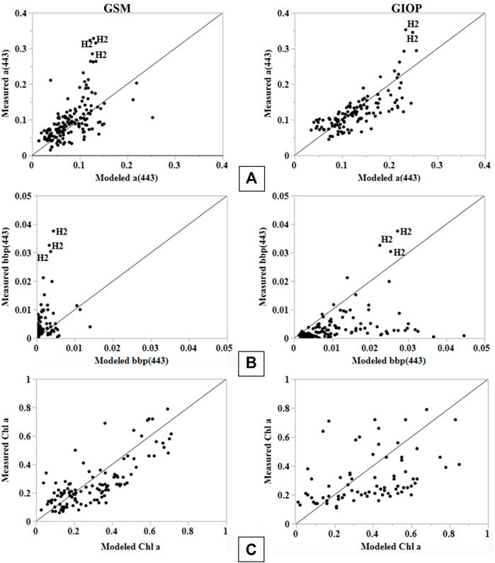
FIGURE 10. Comparison of modeled and in situ (A) a_tot (443) (m⁻¹) (B) b_bp (443) (m⁻¹), and (C) [Chl-a] (µg/L) sampling sites during all field campaigns using GSM (first column), and GIOP (second column) applied to in situ HyperOCR R_rs data. The line represents a 1:1 line.

GSM modeled and in situ a_tot(443) fits reasonably along the 1:1 line. However, the GSM inversion model fails at estimating the IOPs in optically complex turbid waters such as the H2 and MB sites. GSM-based $b_{bp}\left(443\right)$ IOP estimates ranged from 0.001 to 0.011 m⁻¹ with a mean and SE of 0.001 and 0.002 m⁻². The GSM based backscattering values were consistently underestimated, falling below the 1:1 line. This behavior is primarily attributed to the influence of bottom reflectance. Figure 10C shows the correlation plot between modeled and in situ $b_{bp}\left(443\right)$ measurements.

Chl-a estimates from the GSM inversion model ranged from 0.02 to 0.71 μg/L with a mean and SE of 0.3 and 0.02 μg/L respectively. The Chl-a estimates from the GSM model cluster along the 1:1 line against the measured values, with R² = 0.60 and RMSE 0.15. Some overestimated values were at shallow sites such as BI, CR, and MB.

4.3.3 GIOP model

The GIOP inversion model (Werdell et al., 2013) was also applied to Satlantic HyperOCR $R_{rs}$ measurements. The model results were compared with in situ total absorption, particulate backscatter, and Chl-a concentrations. The modeled $a_{tot}\left(443\right)$ ranged from 0.034 to 0.256 m⁻¹ with a mean of 0.13 m⁻¹ and a SE of 0.005 m⁻¹. H2 and CR had the highest average $a_{tot}\left(443\right)$ at 0.23 and 0.21 m⁻¹ with a SE of 0.004 and 0.003 m⁻¹, respectively. This was consistent with in situ $a_{tot}\left(443\right)$ measurements as well as the visually observed conditions during sampling. Consistent with the GSM model, the lowest $a_{tot}\left(443\right)$ estimates were at the offshore HB and NM sites with mean $a_{tot}\left(443\right)$ of 0.05 and 0.06 m⁻¹ with SE of 0.002 and 0.01 m⁻¹, respectively. The performance of the GIOP model against the in situ $a_{tot}\left(443\right)$ is presented Figure 10A. These data have a very similar overall dispersion with GSM a_tot(443) estimates, also showing turbid sites (H2) as outliers. The majority of the a_tot(443) points fall below the 1:1 line suggesting underestimation by the GIOP model. This may be attributed to the $a_{ph}$ basis vector implemented in the default GIOP configuration. GIOP $b_{bp}\left(443\right)$ IOP estimates ranged from 0.001 to 0.045 m⁻¹ with a mean and SE of 0.012 and 0.001 m⁻². These results significantly overestimated in situ b_bp (443) measurements (Figure 10B) and the highest average $b_{bp}\left(443\right)$ estimates were found at CR and H2 (0.023 and 0.017 m⁻¹) which are expected because they are turbid and/or shallow. Low estimates were at the offshore sites HB and NM, consistent with in situ measurements. Chl-a estimates from the GIOP inversion model are more dispersed relative to in situ data (Figure 10C). They ranged from 0 to 0.87 μg/L with a mean and SE of 0.47 and 0.02 μg/L respectively. There was substantial overestimation at almost all sampling sites but particularly at H2, where turbidity was high.

4.3.4 Application of GSM to coincident landsat 8 OLI R_rs

The application of the GSM inversion model to site specific Landsat 8 OLI R_rs produced very similar results to those with from HyperOCR data. The a_tot (443) estimates ranged from 0.048 to 0.151 m⁻¹ with a mean of 0.100 and a SE of 0.005 m⁻¹. Similar to the HyperOCR model results, H2, CR, and MB had the highest a_tot(443) estimates. The modeled a_tot(443) was slightly overestimated (Figure 11A), but estimates generally fell around the 1:1 line with the exception of one sample from H2 acquired on 12/12/2016. This is consistent with other model results where turbid sampling sites did not follow the same trends as sites with clear and deep water. The b_bp(443) estimates from Landsat 8 OLI data were similar to the b_bp (443) results from the GIOP model where they were severely overestimated (Figure 11B). However, the b_bp (443) estimates using HyperOCR data and the GSM model were underestimated. These differences in model results may be due to issues related to atmospheric correction. The Landsat 8 OLI images were corrected for the effects of atmosphere using the 2-band multi-scattering NIR iteration method from Bailey et al. (2010) to remove non-negligible NIR radiance from the NIR signal. However, this could have led to overcorrection resulting in the overestimation of b_bp (443). The Chl-a estimates from Landsat 8 OLI data are very similar to those from HyperOCR data using the GSM model and closely aligned along the 1:1 line (Figure 11C) despite the fact that Chl-a signal is inherently low coupled with the spatial and the slight temporal differences compared to in situ sampling.

FIGURE 11

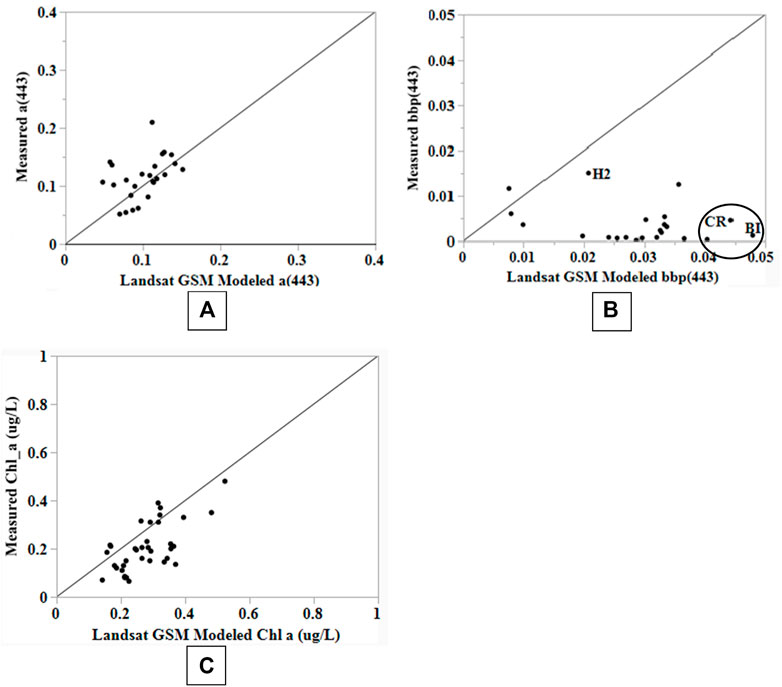
FIGURE 11. Comparison of IOP estimates from the GSM model using Landsat 8 OLI data: total absorption (m^-1) (A), particulate backscatter (m^-1) (B), and Chl-a concentration (µg/L) (C).

Using the GSM model, maps of a_ph(443), a_cdom(443), b_bp(443), and Chl-a concentration are created for each concurrent Landsat 8 image during the study period: 6/3/16, 12/12/16, 5/21/17, 6/6/17, and 6/22/17 (Figure 12). These maps show the spatial variability of IOPs in the nearshore waters of the USVI. Generally, IOP concentrations were higher near the shore, but pixels around clouds and cloud shadows also show high concentrations in some instances. This is due to pixel adjacency effects due to contamination from the clouds and their shadows as opposed to actual IOP concentrations. The highest IOP concentrations occurred on 5/21/2017 (Figure 12C) and could be attributed to the 0.3 cm of precipitation that fell the day before. The lowest concentrations occurred on 12/12/2016 (Figure 12B). Overall, the IOP maps follow the trends observed in in situ measurements.

FIGURE 12

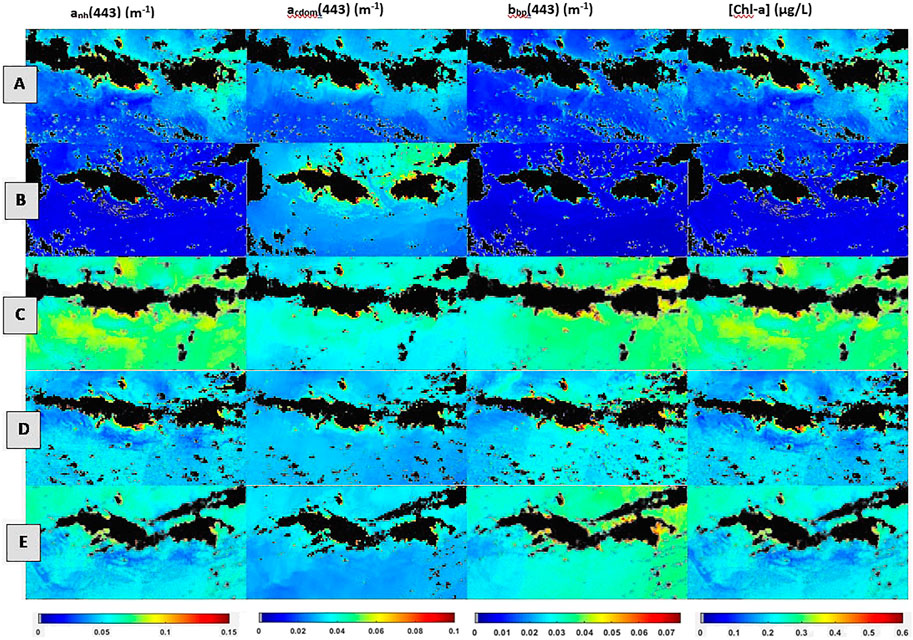
FIGURE 12. The application of the GSM model across a scene encompassing St. Thomas and St. John for concurrent Landsat 8 OLI overpass days: 6/3/16 (A), 12/12/16 (B), 5/21/17 (C), 6/6/17 (D), and 6/22/17 (E).

5 Discussion

5.1 Water quality parameters

The WQPs in the nearshore waters of St. Thomas and St. John varied both spatially and temporally. The variations were influenced by weather conditions such as wind speed, significant wave height, and precipitation. The impacts on water quality from these weather disturbances decreased with distance from shore. In particular, Magens Bay and Charlotte Amalie Harbor were most susceptible to weather events and had the greatest variation in water quality as well as the overall highest average Chl-a concentrations. These locations receive greater quantities of land-based sources of pollution than other sampling sites because the watersheds that feed MB and H2 are some of the most highly developed in the USVI (Kerrigan and Ali, 2020). Higher Chl-a concentrations in these areas are likely due to nutrient enrichment from runoff associated with development within these watersheds. In addition, HB is also a busy port with cruise ships, ferries, and tourist boats introducing and resuspending a significant amount of pollutants and sediment in the Charlotte Amalie Harbor (Kisabeth et al., 2014).

The biogeochemical composition of the nearshore waters of the USVI are best classified as oligotrophic Case-1 waters (Westberry et al., 2005), with optical properties much lower than those typical of turbid Case-2 or optically complex waters (Sathyendranath, 2000; Gitelson et al., 2008; Moses et al., 2009). However, because Chl-a concentrations in the USVI vary depending on precipitation and runoff, the nearshore waters cannot be solely classified as Case 1 waters. The coastal sites such as H2, CR, MB, and FC can be classified as temporally variable Case 2 waters because of their optical properties are controlled by a combination of phytoplankton, and other suspended materials. In contrast, the optical properties of sites further offshore, such as HB, SW, and NM, are primarily controlled by phytoplankton.

Laboratory results indicate that there is a nearshore to offshore gradient in Chl-a concentrations, that follows other water quality trends, such as sedimentation (T. B. Smith et al., 2008). Nearshore sampling sites (H2, MB, BB, BP, and FC) generally had higher Chl-a concentrations than offshore sites (NM, SW, and HB). Other studies have observed these same nearshore to offshore gradients in the USVI (Ennis et al., 2016; Hertler et al., 2009; Kerrigan and Ali, 2020; T. B; Smith et al., 2008). (Ennis et al., 2016) divided the southwestern neritic waters of St. Thomas into three different zones based on perceived anthropogenic impact, some of which correspond to sampling sites in the current study. These previous studies found that Chl-a concentrations were greatest in the areas around Charlotte Amalie Harbor (H2) and measured lower concentrations as the distance from developed watersheds increased. These findings are consistent with our results and suggest that land-based sources of runoff dissipate as they move further offshore.

There were discernable temporal differences in Chl-a concentrations throughout the study period. The seasonal differences in Chl-a concentrations were due to the annual dry and rainy seasons in the USVI. The laboratory measured Chl-a concentrations were higher during the winter sampling campaigns of December 2016 and January/February 2018. These trends suggest that excess amounts of precipitation initiated more runoff than occurs during the summer months causing increased biological activity and primary production. These results are consistent with other studies in the USVI region (Ennis et al., 2016).

5.2 Model applications

5.2.1 Model applications to HyperOCR

As demonstrated in this work as well as in our previous study (Kerrigan et al., 2019) global, empirical algorithms such as OC4 are not suitable for bio-optical conditions in the USVI. These algorithms tend to do perform well in environments where ocean color is primarily a function of single component phytoplankton, and signal-to-noise ratio is high. Neither criterion apply to the USVI coastal waters. The GSM and GIOP inversion models produced slightly different but promising results in retrieving the WQP in the shallow waters of the USVI. For a_tot (443) estimate, the GSM model performed slightly better (R² = 0.55, RMSE = 0.04) than the GIOP (R² = 0.52, RMSE = 0.05) indicating that the GSM model is more effective predictor of a_tot (443) in the USVI. The differences in a_tot (443) model estimates is due to the basis absorption vectors used in the individual models. The GSM model uses basis absorption vectors from the more local, Sargasso Sea which may be responsible for the slightly higher R² and lower RMSE produced by model a_tot(443) estimates. The absorption basis vector in the default configuration of the GIOP model is based on a more global cruise-based data from the Atlantic and Pacific oceans (Bricaud et al., 1998). Both models produced very poor estimates of particulate backscatter (GSM, R² = 0.14 and GIOP, R² = 0.11). The GSM model severely underestimated b_bp (443) and in contrast, the GIOP severely overestimated b_bp(443) (Figure 7). The contrast in performances between the two models is likely due to inherent differences in the particulate backscatter basis vectors used in the modelling and the relatively shallow water conditions with bottom reflectance. The estimates of Chl-a are also a function of the basis vectors applied in the models, hence the observed difference in model Chl-a estimates of the GSM and GIOP. The GSM model performed better (R² = 0.60, RMSE = 0.09) than the GIOP model (R² = 0.17, RMSE = 0.15). The more locally derived GSM model preformed slightly better than the GIOP with respect to atot (443) and much better with respect to Chl-a. Both models performed poorly with respect to bbp (443), although consistent with the trend, the GSM statistics were slightly better for the GSM relative to the GIOP. The poor performance of the GIOP model relative to the GSM model is primarily attributed to the definition of a non-fitting, global-based phytoplankton basis vector used in the GIOP. Low signal-to-noise ratio, bottom signal interference and non-fitting phytoplankton basis vectors, specifically for the semi-analytical models, are the most likely causes of limited performance of the models in the USVI.

5.2.2 GSM application to landsat 8 OLI

The application of the GSM model to Landsat 8 OLI data collected on days in which field sampling took place had good statistical correlation to in situ measurements. Chl-a and a_tot (443) estimates fell very close to the 1:1 line except for some outliers that represent sampling sites with high turbidity and clear, shallow conditions. The GSM based retrieval of Chl-a from Landsat produced R² = 0.45, RMSE = 0.07. The limitations in performance of these models are due to various factors including smaller sample size that match with Landsat pixels, bottom signal interference, boundary conditions, and atmospheric correction errors. The limited number of Landsat 8 scenes (n = 5) during the study period also likely contributed to the high variance and low relative correlation coefficients.

The nature of the nearshore waters in the USVI make it an inherently difficult area for ocean color remote sensing applications. The optically clear water allows sunlight to reach the seafloor contributing to the water leaving radiance and R_rs signal captured by the remote sensing instrument. In the case of the semi-analytical models tested in this study, they were not able to differentiate between the bottom signal contributions and the desired water column reflectance, causing poor performance in retrieving b_bp(443) of the water column constituents. Highly turbid sites (MB, H2, CB) also limited the performance of the semi analytical based IOP retrievals due to the non-linear association of multiple water quality parameters in the water column.

The optical signature from the water only contributes approximately 10%–20% of the total radiance signal measured by the satellite sensor due to the atmospheric path radiance, and in clear, shallow waters such as those found in the USVI, a relatively large portion of the 20% is due to bottom reflectance. This greatly reduces the signal-to-noise ratio of the WQPs. Previous studies in shallow Case I waters have shown that attenuation coefficients can be robustly estimated to depths of approximately 15 m under ideal conditions (Lyzenga, 1981). The majority of the sampling sites in this study (71%) are at depths less than 15 m suggesting that benthic albedo is contributing significantly to the measured R_rs signal.

Because the atmosphere provides such a large contribution to the R_rs signal measured by the satellite sensor, compensation for atmospheric effects is essential for robust ocean color retrievals. In this study, Landsat 8 imagery was corrected for atmosphere using the dark object subtraction (DOS) method (Chavez Jr, 1988) which assumes that dark objects reflect no light, and any reflectance from dark objects is due to atmospheric scattering. The Landsat 8 pixels where sampling sites are located had overall higher reflectance than in situ reflectance measured using the HyperOCR. This suggests that the applied atmospheric effects may not have accounted for all the path radiance. Boundary conditions at the air-sea interface can also greatly affect the reflectance signal measured by satellite sensors. These include wind speed, waves, white caps, and Sun glint. The Landsat 8 imagery used in this study suffered in some areas from specular reflection. Specular reflection occurs when the angle of reflection is equal to the angle of incidence causing the sensor to overestimate actual reflectance values. This could have contributed to the high reflectance values at sampling sites in the Landsat 8 imagery of this study.

6 Conclusion

This study characterized the spatial and temporal variability of WQPs in the nearshore waters of the U.S. Virgin Islands (USVI). Results indicate relatively low concentrations of Chl-a, that varied seasonally and due to acute disturbances. The wet and dry seasons in the USVI area are responsible for small variations in WQPs while larger variations are mainly due to acute disturbances. Acute disturbances included precipitation, high winds, waves, and cruise ships that created large fluxes of nutrient-laden runoff and resuspended sediments. Sampling sites located within the most developed watersheds, Charlotte Amalie Harbor, Magens Bay, and Coral Bay, are most susceptible to these acute disturbances as compared to sites further offshore. Previous research has highlighted the correlation between watershed development and coral reef decline in the USVI (Edmunds and Gray, 2014; Gray et al., 2008; Rogers, 1990; Smith et al., 2014). In-situ optical and physical measurements of the water column are closely associated indicating that ocean color remote sensing is a valuable tool in monitoring changes in the coastal waters of the USVI.

Three empirical and semi-analytical inversion algorithms, namely, OC4, GSM, and GIOP model were evaluated to determine the most robust method for IOP and Chl-a retrievals for coastal waters of the USVI waters. The statistical parameters show that the standard OC4 algorithm perform poorly in the USVI with R2 = 0.14 and RMSE = 0.15. Among the semi-analytical algorithms, the GSM model provides the best retrievals of Chl-a (R² = 0.45, RMSE = 0.07). The differences in the inversion model results are a function of the basis vectors defined within the model framework. The GSM model applied to Landsat 8 OLI imagery showed similar results to the GSM tested on in situ reflectance measurements with moderate a_tot (443) and Chl-a performance (R² = 0.55 and 0.45, respectively) and poor b_bp (443) performance (R² = 0.14). In the USVI, the performance of the ocean color models was also limited due to the contribution of benthic albedo, turbidity in the water column, and the low signal-to-noise ratio of the WQPs.

Data availability statement

The datasets presented in this article are not readily available because will be submitted to SeaBASS datasets. Requests to access the datasets should be directed to alika@cofc.edu.

Author contributions

KA, DF, MB, and JO were involved in the research cruise and field data collection. Data analysis and writing of the paper was done primarily by KA and DF, MB, JO, and TS contributed in analysis, interpretation and reviewing steps. All authors contributed to the article and approved the submitted version.

Funding

This research is funded by NASA Biological and Physical Sciences Division under the NASA EPSCOR Program, NASA Grant Number NNX15AM74A.

Acknowledgments

This work includes results from part of a master’s thesis work by DF at the college of Charleston, we would like to thank his thesis committee for reviewing the work.

Conflict of interest

The authors declare that the research was conducted in the absence of any commercial or financial relationships that could be construed as a potential conflict of interest.

Publisher’s note

All claims expressed in this article are solely those of the authors and do not necessarily represent those of their affiliated organizations, or those of the publisher, the editors and the reviewers. Any product that may be evaluated in this article, or claim that may be made by its manufacturer, is not guaranteed or endorsed by the publisher.

References

Ali, K. A., Witter, D. L., and Ortiz, J. D. (2014). Multivariate approach to estimate colour producing agents in Case 2 waters using first-derivative spectrophotometer data. Geocarto Int. 29, 102–127. doi:10.1080/10106049.2012.743601

CrossRef Full Text | Google Scholar

Arar, E. J., and Collins, G. B. (1997). Method 445.0: In vitro determination of chlorophyll a and pheophytin a in marine and freshwater algae by fluorescence. United States Environmental Protection Agency, Office of Research and Development, National Exposure Research Laboratory.

Brandt, M. E., Smith, T. B., Correa, A. M. S., and Vega-Thurber, R. (2013). Disturbance driven colony fragmentation as a driver of a coral disease outbreak. PLoS One 8 (2), e57164. doi:10.1371/journal.pone.0057164

PubMed Abstract | CrossRef Full Text | Google Scholar

Bailey, S. W., Franz, B. A., and Werdell, P. J. (2010). Estimation of near-infrared water-leaving reflectance for satellite ocean color data processing. Optics Express 18 (7), 7521–7527.

PubMed Abstract | CrossRef Full Text | Google Scholar

Bricaud, A., Morel, A., Babin, M., Allali, K., and Claustre, H. (1998). Variations of light absorption by suspended particles with chlorophyll a concentration in oceanic (case 1) waters: Analysis and implications for bio-optical models. J. Geophys. Res. Oceans 103 (C13), 31033–31044. doi:10.1029/98jc02712

CrossRef Full Text | Google Scholar

Bruno, J. F., Petes, L. E., Drew Harvell, C., and Hettinger, A. (2003). Nutrient enrichment can increase the severity of coral diseases. Ecol. Lett. 6 (12), 1056–1061. doi:10.1046/j.1461-0248.2003.00544.x

CrossRef Full Text | Google Scholar

Bruno, J. F., and Selig, E. R. (2007). Regional decline of coral cover in the indo-pacific: Timing, extent, and subregional comparisons. PLoS One 2 (8), e711. doi:10.1371/journal.pone.0000711

PubMed Abstract | CrossRef Full Text | Google Scholar

Burke, L., Reytar, K., Spalding, M., and Perry, A. (2011). Reefs at risk revisited. Washington, DC: World Resources Institute.

Google Scholar

Chavez, P. S. (1988). An improved dark-object subtraction technique for atmospheric scattering correction of multispectral data. Remote Sens. Environ. 24 (3), 459–479. doi:10.1016/0034-4257(88)90019-3

CrossRef Full Text | Google Scholar

Clay, S., Peña, A., DeTracey, B., and Devred, E. (2019). Evaluation of satellite-based algorithms to retrieve chlorophyll-a concentration in the Canadian Atlantic and Pacific oceans. Remote Sens. 11 (22), 2609. doi:10.3390/rs11222609

CrossRef Full Text | Google Scholar

Cunning, R., and Baker, A. C. (2013). Excess algal symbionts increase the susceptibility of reef corals to bleaching. Nat. Clim. Change 3 (3), 259–262. doi:10.1038/nclimate1711

CrossRef Full Text | Google Scholar

De’Ath, G., Fabricius, K. E., Sweatman, H., and Puotinen, M. (2012). The 27–year decline of coral cover on the Great Barrier Reef and its causes. Proc. Natl. Acad. Sci. 109 (44), 17995–17999. doi:10.1073/pnas.1208909109

CrossRef Full Text | Google Scholar

Edmunds, P. J., and Gray, S. C. (2014). The effects of storms, heavy rain, and sedimentation on the shallow coral reefs of St. John, US Virgin Islands. Hydrobiologia 734, 143–158. doi:10.1007/s10750-014-1876-7

CrossRef Full Text | Google Scholar

Ennis, R. S., Brandt, M. E., Grimes, K. R. W., and Smith, T. B. (2016). Coral reef health response to chronic and acute changes in water quality in St. Thomas, United States Virgin Islands. Mar. Pollut. Bull. 111 (1–2), 418–427. doi:10.1016/j.marpolbul.2016.07.033

PubMed Abstract | CrossRef Full Text | Google Scholar

Fabricius, K. E. (2005). Effects of terrestrial runoff on the ecology of corals and coral reefs: Review and synthesis. Mar. Pollut. Bull. 50 (2), 125–146. doi:10.1016/j.marpolbul.2004.11.028

PubMed Abstract | CrossRef Full Text | Google Scholar

Furnas, M., Mitchell, A., Skuza, M., and Brodie, J. (2005). In the other 90%: Phytoplankton responses to enhanced nutrient availability in the great barrier reef lagoon. Mar. Pollut. Bull. 51 (1–4), 253–265. doi:10.1016/j.marpolbul.2004.11.010

PubMed Abstract | CrossRef Full Text | Google Scholar

Gattuso, J. P., Hoegh-Guldberg, O., and Pörtner, H. O. (2014). “Cross-chapter box on coral reefs,” in Climate change 2014: Impacts, adaptation, and vulnerability. Part A: Global and sectoral aspects. Contribution of working Group II to the fifth assessment report of the intergovernmental panel of climate change (Cambridge University Press, Cambridge), 97–100.

Google Scholar

Gitelson, A. A., Dall’Olmo, G., Moses, W., Rundquist, D. C., Barrow, T., Fisher, T. R., et al. (2008). A simple semi-analytical model for remote estimation of chlorophyll-a in turbid waters: Validation. Remote Sens. Environ. 112 (9), 3582–3593. doi:10.1016/j.rse.2008.04.015

CrossRef Full Text | Google Scholar

Gordon, H. R., Brown, O. B., Evans, R. H., Brown, J. W., Smith, R. C., Baker, K. S., et al. (1988). A semianalytic radiance model of ocean color. J. Geophys. Res. Atmos. (1984–2012), 93(D9), 10909–10924. doi:10.1029/jd093id09p10909

CrossRef Full Text | Google Scholar

Gordon, H. R., and Wang, M. (1994). Retrieval of water-leaving radiance and aerosol optical thickness over the oceans with SeaWiFS: a preliminary algorithm. Appl. Opt., 33(3), 443. doi:10.1364/ao.33.000443

PubMed Abstract | CrossRef Full Text | Google Scholar

Gray, S. C., Gobbi, K. L., and Narwold, P. V. (2008). Comparison of sedimentation in bays and reefs below developed versus undeveloped watersheds on St. John. US Virgin Islands, 351–356.

Google Scholar

Gray, Sarah C., Sears, W., Kolupski, M. L., Hastings, Z. C., Przyuski, N. W., Fox, M. D., et al. (2012). Factors affecting land-based sedimentation in coastal bays, US Virgin Islands. Proceedings of the 12th International Coral Reef Symposium (James Cook University, Australia)July 2012, 9–13.

Google Scholar

Hertler, H., Boettner, A. R., Ramírez-Toro, G. I., Minnigh, H., Spotila, J., and Kreeger, D. (2009). Spatial variability associated with shifting land use: Water quality and sediment metals in La Parguera, Southwest Puerto Rico. Mar. Pollut. Bull. 58 (5), 672–678. doi:10.1016/j.marpolbul.2009.01.018

PubMed Abstract | CrossRef Full Text | Google Scholar

Hoegh-Guldberg, O. (2011). Coral reef ecosystems and anthropogenic climate change. Reg. Environ. Change 11, 215–227. doi:10.1007/s10113-010-0189-2

CrossRef Full Text | Google Scholar

Hoegh-Guldberg, O., Mumby, P. J., Hooten, A. J., Steneck, R. S., Greenfield, P., Gomez, E., et al. (2007). Coral reefs under rapid climate change and ocean acidification. Science 318 (5857), 1737–1742. doi:10.1126/science.1152509

PubMed Abstract | CrossRef Full Text | Google Scholar

Hoegh-Guldberg, O., Poloczanska, E. S., Skirving, W., and Dove, S. (2017). Coral reef ecosystems under climate change and ocean acidification. Front. Mar. Sci. 4, 158. doi:10.3389/fmars.2017.00158

CrossRef Full Text | Google Scholar

Hubbard, D. K. (1987). Virgin Islands resource management cooperative. Biosphere reserve research report.

Google Scholar

Hughes, T. P. (1994). Catastrophes, phase shifts, and large-scale degradation of a Caribbean coral reef. Science 265 (5178), 1547–1551. doi:10.1126/science.265.5178.1547

PubMed Abstract | CrossRef Full Text | Google Scholar

Kerrigan, K., and Ali, K. A. (2020). Application of Landsat 8 OLI for monitoring the coastal waters of the US Virgin Islands. Int. J. Remote Sens. 41 (15), 5743–5769. doi:10.1080/01431161.2020.1731770

CrossRef Full Text | Google Scholar

Kisabeth, J. K., Smith, T., Primack, A., and Wilson, K. (2014). Cruise ship induced sediment resuspension characteristics in Charlotte Amalie harbor and the west gregerie channel. St. Thomas, US Virgin Islands: University of the Virgin Islands.

Google Scholar

Klemas, V. (2011). Remote sensing techniques for studying coastal ecosystems: An overview. J. Coast. Res. 27 (1), 2–17. doi:10.2112/JCOASTRES-D-10-00103.1

CrossRef Full Text | Google Scholar

Lee, Z., Carder, K. L., and Arnone, R. A. (2002). Deriving inherent optical properties from water color: A multiband quasi-analytical algorithm for optically deep waters.

Google Scholar

Lewis, K. M., and Arrigo, K. R. (2020). ocean color algorithms for estimating chlorophyll a, CDOM absorption, and particle backscattering in the arctic ocean. J. Geophys. Res. Oceans 125 (6). doi:10.1029/2019JC015706

CrossRef Full Text | Google Scholar

Lyzenga, D. R. (1981). Remote sensing of bottom reflectance and water attenuation parameters in shallow water using aircraft and Landsat data. Int. J. Remote Sens. 2 (1), 71–82. doi:10.1080/01431168108948342

CrossRef Full Text | Google Scholar

Maritorena, S., Siegel, D. A., and Peterson, A. R. (2002). Optimization of a semianalytical ocean color model for global-scale applications. Appl. Opt. 41 (15), 2705–2714. doi:10.1364/ao.41.002705

PubMed Abstract | CrossRef Full Text | Google Scholar

McClain, C. R. (2009). A decade of satellite ocean color observations. Annu. Rev. Mar. Sci. 1, 19–42. doi:10.1146/annurev.marine.010908.163650

PubMed Abstract | CrossRef Full Text | Google Scholar

Miller, J. A., Whitehead, R. L., Oki, D. S., Gingerich, S. B., and Olcott, P. G. (1997). Ground water atlas of the United States: Segment 13, Alaska, Hawaii, Puerto Rico, and the US Virgin Islands. US geological survey.

Google Scholar

Moses, W. J., Gitelson, A. A., Berdnikov, S., and Povazhnyy, V. (2009). Satellite estimation of Chlorophyll-$a$ concentration using the red and NIR bands of meris—the azov sea case study. Geoscience Remote Sens. Lett. IEEE 6 (4), 845–849. doi:10.1109/lgrs.2009.2026657

CrossRef Full Text | Google Scholar

O’Reilly, J. E., Maritorena, S., Mitchell, B. G., Siegel, D. A., Carder, K. L., Garver, S. A., et al. (1998). Ocean color chlorophyll algorithms for SeaWiFS. J. Geophys. Res. Oceans 103 (C11), 24937–24953. doi:10.1029/98jc02160

CrossRef Full Text | Google Scholar

O’Reilly, J. E., Maritorena, S., Siegel, D. A., O’Brien, M. C., Toole, D., Mitchell, B. G., et al. (2000). Ocean color chlorophyll a algorithms for SeaWiFS, OC2, and OC4: Version 4. SeaWiFS Postlaunch Calibration Validation Analyses, Part 3, 9–23.

Google Scholar

O’Reilly, J. E., and Werdell, P. J. (2019). Chlorophyll algorithms for ocean color sensors—OC4, OC5 & OC. Remote Sens. Environ. 229, 32–47. doi:10.1016/j.rse.2019.04.021

PubMed Abstract | CrossRef Full Text | Google Scholar

Pope, R. M., and Fry, E. S. (1997). Absorption spectrum (380–700 nm) of pure water. II. Integrating cavity measurements. Appl. Opt. 36 (33), 8710–8723. doi:10.1364/ao.36.008710

PubMed Abstract | CrossRef Full Text | Google Scholar

Ramos-Scharrón, C. E., and LaFevor, M. C. (2016). The role of unpaved roads as active source areas of precipitation excess in small watersheds drained by ephemeral streams in the Northeastern Caribbean. J. Hydrology 533, 168–179. doi:10.1016/j.jhydrol.2015.11.051

CrossRef Full Text | Google Scholar

Roesler, C. S., and Perry, M. J. (1995). In situ phytoplankton absorption, fluorescence emission, and particulate backscattering spectra determined from reflectance. J. Geophys. Res. Oceans 100 (C7), 13279–13294. doi:10.1029/95jc00455

CrossRef Full Text | Google Scholar

Rogers, C. S. (1990). Responses of coral reefs and reef organisms to sedimentation. Mar. Ecol. Prog. Ser. Oldend. 62 (1), 185–202. doi:10.3354/meps062185

CrossRef Full Text | Google Scholar

Rothenberger, P., Blondeau, J., Cox, C., Curtis, S., Fisher, W. S., Garrison, V., et al. (2008). The state of coral reef ecosystems of the US Virgin Islands, The state of coral reef ecosystems of the United States and Pacific Freely Associated States 73. NOAA Center for Coastal Monitoring and Assessment’s Biogeography Team Silver, 29–73.

Google Scholar

Sathyendranath, S. (2000). Reports of the international ocean-colour coordinating Group, 3. Dartmouth, Canada: IOCCG, 140.

Google Scholar

Schwartz, M. (2010). Encyclopedia of the world’s coastal landforms, Virgin Islands: Springer.

Google Scholar

Smith, J. E., Shaw, M., Edwards, R. A., Obura, D., Pantos, O., Sala, E., et al. (2006). Indirect effects of algae on coral: Algae-mediated, microbe-induced coral mortality. Ecol. Lett. 9 (7), 835–845. doi:10.1111/j.1461-0248.2006.00937.x

PubMed Abstract | CrossRef Full Text | Google Scholar

Smith, R. C., and Baker, K. S. (1981). Optical properties of the clearest natural waters (200–800 nm). Appl. Opt. 20 (2), 177–184. doi:10.1364/ao.20.000177

PubMed Abstract | CrossRef Full Text | Google Scholar

Smith, T. B., Ennis, R. S., Brown, K., and Wright, V. (2014). Study of nutrient analysis and distribution and sedimentation rate: Phase II. US Virgin Islands Department of Environmental Protection. Section 106 Research Program.

Google Scholar

Smith, T. B., Nemeth, R. S., Blondeau, J., Calnan, J. M., Kadison, E., and Herzlieb, S. (2008). Assessing coral reef health across onshore to offshore stress gradients in the US Virgin Islands. Mar. Pollut. Bull. 56 (12), 1983–1991. doi:10.1016/j.marpolbul.2008.08.015

PubMed Abstract | CrossRef Full Text | Google Scholar

Vega Thurber, R. L., Burkepile, D. E., Fuchs, C., Shantz, A. A., McMinds, R., and Zaneveld, J. R. (2014). Chronic nutrient enrichment increases prevalence and severity of coral disease and bleaching. Glob. Change Biol. 20 (2), 544–554. doi:10.1111/gcb.12450

CrossRef Full Text | Google Scholar

Walling, D. E. (1997). The response of sediment yields to environmental change, 245. IAHS Publication, Wallingford UK, 77–89.

Google Scholar

Weber, M., De Beer, D., Lott, C., Polerecky, L., Kohls, K., Abed, R. M. M., et al. (2012). Mechanisms of damage to corals exposed to sedimentation. Proc. Natl. Acad. Sci. 109 (24), E1558–E1567. doi:10.1073/pnas.1100715109

PubMed Abstract | CrossRef Full Text | Google Scholar

Werdell, P. J., Franz, B. A., Bailey, S. W., Feldman, G. C., Boss, E., Brando, V. E., Dowell, M., Hirata, T., Lavender, S. J., and Lee, Z. (2013). Generalized ocean color inversion model for retrieving marine inherent optical properties. Applied Optics, 52 (10), 2019–2037.

PubMed Abstract | CrossRef Full Text | Google Scholar

Werdell, P. J., and McKinna, L. I. W. (2019). Sensitivity of inherent optical properties from ocean reflectance inversion models to satellite instrument wavelength suites. Front. Earth Sci. 7, 54. doi:10.3389/feart.2019.00054

PubMed Abstract | CrossRef Full Text | Google Scholar

Westberry, T. K., Siegel, D. A., and Subramaniam, A. (2005). An improved bio-optical model for the remote sensing of Trichodesmium spp. blooms. J. Geophys. Res. Oceans 110 (C6), C06012. doi:10.1029/2004jc002517

CrossRef Full Text | Google Scholar