Spectral imaging of grass species in arid ecosystems of Namibia

1 Introduction

The decade from 2021 to 2030 has been designated by the United Nations as the Decade of Ecosystem Restoration worldwide, with the aim to achieve the Sustainable Development Goals (SDG) by 2030 (UN Decade on Restoration, 2023). As one of the most widespread ecosystems, covering approximately 30%–40% of the Earth’s land surface and occurring on every continent except Antarctica, restoration activities should particularly focus on grasslands, especially in achievement of SDG 15 (Blair et al., 2014; Latham et al., 2014). SDG 15 focuses on protecting, restoring and promoting the sustainable use of terrestrial ecosystems, sustainable forest management, combating desertification, halting and reversing land degradation and halting biodiversity loss (United Nations, 2023). Grasslands can be defined as heterogenous and biodiversity rich areas where vegetation consists almost exclusively of grasses (Poaceae) with occasional trees and shrubs, which fulfil both ecological and cultural functions (Gibson, 2009; Petermann and Buzhdygan, 2021). Ecosystem services provided by grasslands include water supply and flow regulation, erosion control, forage for livestock and wildlife, carbon sequestration, medicinal plants and other cultural services (Derner and Schuman, 2007; Bengtsson et al., 2019; Zhao et al., 2020; Kleppel and Frank, 2022; Kose et al., 2022). Globally, grasslands have both degraded and improved over the last decades as a result of regional impacts of climate change and human activities (Gang et al., 2014; Yan et al., 2023). Most of the global grassland degradation has occurred in Africa, particularly in tropical and southern drylands (Yan et al., 2023). Besides climate change and human activities, dryland grassland degradation is increasing due to grazing pressure, often unrecognized in national and international policies (Bardgett et al., 2021; Maestre et al., 2022). Grasslands also receive less scientific attention than other terrestrial ecosystems such as wetlands and forests (Temperton et al., 2019; Török et al., 2021). According to Zhao et al., 2020, there is a need for future research efforts that consider grasslands more holistically, taking into account pressure, state and response, and using a multi-scale, multi-method and multi-perspective approach. Remote sensing can provide a substantial contribution to monitor grassland ecosystem dynamics at different spatio-temporal scales including phenological states, distribution of grassland types, biomass, biodiversity and forage quality (Ali et al., 2016; Gamon et al., 2019; Zhao et al., 2020). Regional focuses of remote sensing based grassland research can be identified in Asia, especially China, North America, Western and Southern Europe, Australia and South Africa, while for much of the rest of the world, including Namibia, there are no or only scattered studies available (Reinermann et al., 2020; Masenyama et al., 2022). Most common multispectral sensors, but also radar sensors have been used to analyze grasslands, but the advent of the new generation of spaceborne imaging spectrometers opens new possibilities for grassland monitoring in future (Reinermann et al., 2020; Ferner et al., 2021; Masenyama et al., 2022). The advantage of hyperspectral remote sensing or imaging spectroscopy compared to multispectral data is that data is acquired in quasi-continuous narrow bands rather than broad bands, resulting in much higher spectral resolution and thus a laboratory-like spectrum for each pixel, allowing better detection of surface materials and their qualitative properties (Goetz et al., 1985; Schaepman, 2007). Since Alexander Goetz pioneered the first airborne imaging spectrometer in the 1990s, hyperspectral remote sensing has continued to develop, and in 2000 the Earth Observing-1 satellite (EO-1) was launched, carrying the first spaceborne imaging spectrometer, Hyperion (Vane et al., 1984; Goetz et al., 1985; Ungar, 2001; Pearlman et al., 2003; Ustin et al., 2004; MacDonald et al., 2009). Since then, several spaceborne imaging spectrometers have been launched. Some examples of new generations are the German DLR Earth Sensing Imaging Spectrometer (DESIS), the Italian PRecursore IperSpettrale della Missione Applicativa (PRISMA), the Japanese Hyperspectral Imager Suite (HISUI) or the German Environmental Mapping and Analysis Program (EnMAP) (Rast and Painter, 2019). To validate remote sensing data, field spectroscopy is one of the most commonly used methods to collect in situ data, which is fast, non-destructive and can measure biophysical parameters (Ali et al., 2016; Masenyama et al., 2022). When combined with remote sensing data, field spectra contribute to a better understanding of plant biodiversity and forage quality on a larger scale (Cavender-Bares et al., 2017; Dao et al., 2021). Vegetation spectra typically cover the spectral range of 380–2,500 nm where the characteristic absorption features are located (Kokaly et al., 2009; Ustin et al., 2009; Homolová et al., 2013). These include the absorption of leaf photosynthetic pigments such as chlorophylls (400–700 nm), leaf structure (700–1,300 nm), especially plant water around 950–970 nm, and water absorption and biochemicals such as protein (1,300–2,500 nm) (Peñuelas et al., 1993; Homolová et al., 2013; Gamon et al., 2019). Spectral libraries are databases of spectra of various vegetation, minerals, materials, etc., designed to facilitate laboratory and field spectroscopy and remote sensing and to make these spectra available for applications beyond case studies (Ruby and Fischer, 2002; Jiménez and Díaz-Delgado, 2015). However, spectral information on individual species is limited worldwide, with only few spectral libraries containing grass spectra (Jetz et al., 2016). Less than 30 grass spectra were found in the United States Geological Survey (USGS) Spectral Library Version seven and only a few spectral libraries published in the Ecological Spectral Information System (EcoSIS) contained grass spectra, mostly from United States, Belgium or Brazil (Schweiger, 2016a; 2016b; Dennison and Gardner, 2016; Kokaly et al., 2017; Dennison et al., 2019a; 2019b; Wang, 2019a; 2019b; 2019c; Van Cleemput et al., 2019; Van Cleemput et al., 2020; Wang et al., 2021; Wang, 2022a; 2022b). Only one spectral library contained grass spectra from southern Africa (Frye et al., 2021). According to Ferner et al., 2021, neither hyperspectral nor multispectral imagery combined with field spectroscopy provide optimal results on the quality of African savanna grasslands, but this may change in future with the advent of new generation of spaceborne imaging spectrometers. In southern Africa, past studies of grassland quality have often focused on eastern South Africa, using field spectra, multispectral and airborne hyperspectral data (Knox et al., 2011; Ramoelo et al., 2011; Ramoelo et al., 2012; Ramoelo et al., 2013; Singh et al., 2017). In addition, few studies in recent decades have used these data to examine grasslands in the more semi-arid areas of Namibia (Deshmukh, 1984; Oldeland et al., 2010; Juergens et al., 2013; Shikangalah and Mapani, 2020; Amputu et al., 2022; Männer et al., 2022; Amputu et al., 2023). In particular, research on arid grasslands using imaging spectroscopy has been limited to North America and Mongolia (Van Cleemput et al., 2018). According to Okin et al., 2001, the study of vegetation in drylands is particularly challenging because drought results in less meaningful vegetation spectra, making it difficult to separate and unmix, and can lead to over-interpretation of vegetation cover. The same challenge applies to Namibia, where highly variable and unpredictable rainfall, combined with multi-year droughts, has a strong impact on grasslands (Shikangalah, 2020; Liu and Zhou, 2021; Mendelsohn and Mendelsohn, 2022). As a result of climate change and associated desertification and bush encroachment, Namibian grasslands are expected to be replaced by deserts and arid shrublands as the predominant form of vegetation (Midgley et al., 2005; Dirkx et al., 2008). This study focuses on two private reserves located within the Greater Sossusvlei-Namib Landscape, namely, the NamibRand Nature Reserve (NRNR) and ProNamib Nature Reserve (PNNR), aiming at holistic biodiversity conservation including grassland restoration measures (NamibRand Nature Reserve, 2023; ProNamib Nature Reserve, 2023). The aim of this research is to effectively support both reserves by mapping the status quo of grassland. First mapping and measurement activities were conducted during a field campaign in March 2023, which forms the basis for future monitoring. Additionally, results are compared to a vegetation survey by Burke, 2022 to provide insight into grassland dynamics. In addition, this work aims to contribute to the identified research gaps on arid grasslands in southern Africa and particularly in Namibia. A unique spectral library has been created to describe spectra of common soil, grass and shrub species and to investigate intra-species spectral homogeneity and inter-species spectral separability. This will be used to determine the impact of challenges described by Okin et al., 2001 on separability and unmixing of vegetation spectra in drylands. Furthermore, a multi-sensor remote sensing approach will be tested using the latest generation of hyperspectral data (PRISMA and EnMAP), Sentinel-2 as a publicly available multispectral dataset and PlanetScope SuperDove as a high spatial resolution but commercial multispectral dataset. A suitable approach will be developed to combine this data with field spectra, for first-time mapping of grasslands and to identify limitations and advantages of each dataset. This addresses the research gap identified by Ferner et al., 2021, as to whether multispectral or hyperspectral data are more appropriate to explore grassland, especially within arid ecosystems. In addition, a data fusion product will be compared to verify the assertion of Ghamisi et al., 2019 that data fusion improves target identification. Finally, the knowledge gained from these objectives will be used to enable holistic and spatio-temporal monitoring of grassland ecosystem dynamics in the Greater Sossusvlei-Namib Landscape in future.

2 Materials and methods

This chapter provides an overview of the study area and the process of field data collection before detailing the processing steps required to achieve the stated objectives.

2.1 Study area

The NRNR and PNNR are part of the Greater Sossusvlei-Namib Landscape and are located between the Namib Naukluft National Park and the Nubib Mountains at the edge of Namib Sand Sea in the Hardap region of Namibia (Figures 1A, B). AccAording to NamibRand Nature Reserve, 2023; ProNamib Nature Reserve, 2023, both were established on former farmland and are currently surrounded by livestock farms. The relatively new PNNR, which can be seen as an eastern extension, was established in 2020, while the NRNR has been in existence for over 30 years. Objectives of both reserves are very similar: To increase biomass, restore grasslands and create a functional and biodiverse ecosystem. For this purpose, remaining fences of former farms were removed to facilitate wildlife migration and protect the unique ecology and wildlife. Differences consist in the way tourism is managed. PNNR aims to reduce human impact and plans to largely avoid tourism, whilst NRNR relies on high quality, low impact tourism for its funding. NRNR, one of the largest privately-owned nature reserves in Southern Africa, encompasses an area of around 1,700 km². PNNR, covering approximately 680 km², plans to expand to match NRNR’s size in future. Fieldwork was conducted in both reserves. The study’s area of interest (AOI) is approximately 760 km² and covered by all satellite sensors allowing a multi-sensor approach. The AOI comprises around 426 km² of PNNR and about 334 km² of surrounding livestock farmland. (Figure 1A). According to Mendelsohn and Mendelsohn, 2022, growing season and productivity of vegetation, especially grasses, in Namibia are particularly dependent on rainfall, which is highly variable, unpredictable, and strongly influenced by the El Niño Southern Oscillation. The rainy season lasts from October to March and the growing season from December to May. Based on Mendelsohn and Mendelsohn, 2022, the climate in the study area is classified as arid with average annual temperatures between 19°C and 21°C. In addition, precipitation in the study area varies due to an increasing rainfall gradient from west to east. The average annual rainfall (1993–2022) of PNNR, is 102 mm, while NRNR shows an average of only 43 mm respectively (Figure 1C). Most of the precipitation occurs in the months of January to March (Figure 1C). The variability of precipitation between years is evident with the wettest year in 2011 (185 mm of rainfall in PNNR and 87 mm in NRNR), and the driest year in 2019 (48 mm of rainfall in PNNR and 20 mm in NRNR). After two very good rainy seasons in 2021 and 2022, the first months of 2023 had only slightly more precipitation than in 2019. Besides precipitation, the second dominant factor for vegetation growth is substrate. The predominant soil types, apart from sandy dunes, are leptosols and regosols, whose formation depends on the adjacent geology (Burke, 2022; Mendelsohn and Mendelsohn, 2022). In general, the geology of the area can be divided into three areas: The escarpment in the east with sandstone, sedimentary rocks and limestone of the Nama formation, various rock types of the Namaqua Metamorphic Complex prevailing in the east and south and granites in the northern, western and central parts of the reserves (Miller, 2008; Burke, 2022). The elevation ranges from nearly 500 m in the northwest of NRNR to around 2000 m above sea level, with the highest mountains in the East central part near the northern border between both reserves (German Aerospace Center, 2022). The most recent vegetation survey of both reserves was conducted in 2022, during a period of very high rainfall, when over 250 plant species in 11 different vegetation types were recorded (Burke, 2022). Most dominant grass species were the sour grass Schmidtia kalihariensis (annual) and the bushman grasses Stipagrostis ciliata, Stipagrostis obtusa and Stipagrostis uniplumis (all perennial) (Burke, 2022; van Oudtshoorn, 2022). Other dominant vegetation species included the shrubs Boscia foetida, Calicorema capitata, Lycium bosciifolium, Monechma cleomoides, Petalidium setosum and Rhigozum trichotomum, the acacia Acacia erioloba and the herb Gisekia africana (Burke, 2022).

FIGURE 1

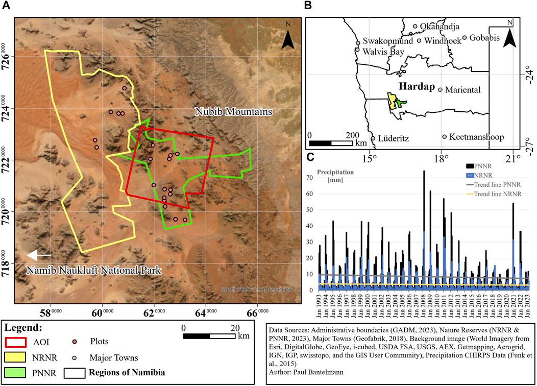
FIGURE 1. Location of the study area. (A) Area of Interest (AOI) and Nature Reserves with plots of fieldwork, although not all 35 plots are recognizable due to overlap. (B) Location of NRNR and PNNR incl. neighboring livestock farms within Namibia. (C) Precipitation data monthly aggregated for NRNR and PNNR from Climate Hazards Group InfraRed Precipitation with Station data (CHIRPS) with trend lines. CHIRPS data was analyzed using Google Earth Engine (Gorelick et al., 2017). Trend lines over the 30-year period are shown in grey for PNNR and yellow for NRNR. Additional CHIRPS data on total annual precipitation and annual precipitation in the first 3 months (January to March) of each year for the period 1993 to 2023 are presented in Supplementary Table S1.

2.2 Field work

Fieldwork was carried out in both reserves from 11 to 17 March 2023 between 8 a.m. and 5 p.m. under clear skies. A total of 42 spectra were collected from 35 one-square-meter plots selected according to topography and vegetation greenness. The data collected at each plot was documented in a study-specific protocol, which can be found in the appendix (Supplementary Figure S1). Waypoint averaging feature of the Garmin GPSMAP 60CSx handheld GPS unit was used to measure the plots with an inaccuracy of less than 10 m (Garmin International Inc, 2005). Books by Müller, 2007; Burke, 2008, 2009a, 2009b; Roodt, 2015; van Oudtshoorn, 2022 were used to identify species in the field, but no distinction was possible between individual variations, e.g., Stipagrostis uniplumis and the variations var. uniplumis, neesii or intermedia. Field spectra were measured using an Analytical Spectral Devices FieldSpec 3, which records the radiant energy using three different detectors (VNIR [350–1,000 nm], SWIR 1 [1,000–1830 nm] and SWIR 2 [1830–2,500 nm]) with a spectral resolution of 3–10 nm (Analytical Spectral Devices Inc., 2010a, Boulder, Colorado, United States). The protocol of Kalacska et al., 2018 was applied to standardize field measurements of spectra. The spectroradiometer was recalibrated before each measurement using dark current and white reference correction. The white reference correction for pistol measurements was performed on a 95% white reference (SphereOptics, 2022, Herrsching am Ammersee, Germany: ID. NO: SG3151). For pistol measurements, the pistol was held in a nadir position 1 m above the canopy with a 25° field of view. The solar height during the measurements ranged from 30 to 90°. It was not possible to measure exclusively at zenith due to high temperatures above 40°C and the temporary failure of our instruments around midday. For contact measurements, the blade, sheath and internode were clamped and jointly measured using the Analytical Spectral Devices Leaf Clip (Analytical Spectral Devices Inc., 2010b., Boulder, Colorado, United States). The two programs RS3 and ViewSpec Pro were used to check the spectra for measurement errors in field (Analytical Spectral Devices Inc, 2008a; Analytical Spectral Devices Inc, 2008b., Boulder, Colorado, United States). Spectral measurements by contact and pistol were focused on grasses, but also included selected shrubs. Plots with poor vegetation were measured by contact only, and soils were generally measured close to selected plots by pistol only. For each plot and measurement type, 10 replicates were measured. The output data for each spectrum were reflectance values interpolated to 1 nm spectral resolution. Each spectra was stored in a single. asd file. In addition to soil spectra, soil color, clay content and particle size of topsoil (relevant for this approach) were evaluated using Munsell Soil Color Chart Book and World Reference Base for Soil Resources (Munsell Color Corporation, 2009; International Union of Soil Sciences, 2022).

2.3 Data processing

A suitable approach for combining the field spectra with the selected satellite data is shown in Figure 2 and includes all necessary processing and analysis steps, which are described in detail in the following chapter.

FIGURE 2

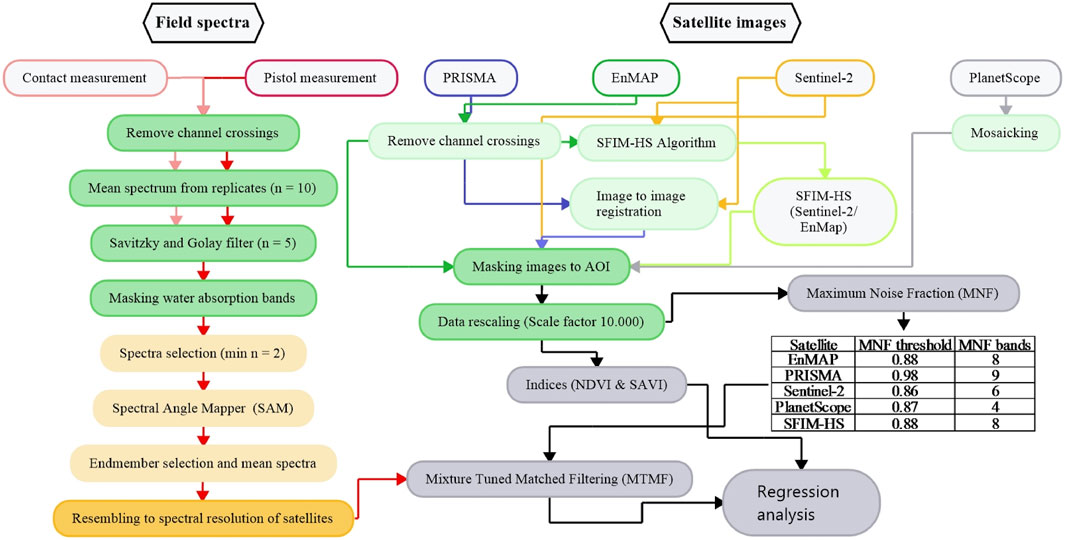
FIGURE 2. Workflow diagram. Light grey: Input data; Light green: Individual preprocessing steps; Green: General preprocessing steps; Light yellow: Endmember selection; Yellow: Endmember resembling; Grey: unmixing using spectral hourglass wizard and regression analyses using selected indices. Arrow colors correspond to input data contours, with black arrows representing processes that are common to all satellite data and colored arrows representing processes that are specific to input data, e.g., blue arrows for PRISMA. SFIM-HS is the abbreviation for the generated data fusion product based on the Smoothing Filter-based Intensity Modulation hypersharpening method, which is described in more detail in chapter 2.3.2 Description and pre-processing of satellite data.

2.3.1 Pre-processing field spectra

The field spectra were preprocessed using R version 4.3.0 and the packages hsdar, hyperSpec, asdreader and RStoolbox (Roudier, 2017; Lehnert et al., 2019; Beleites and Sergo, 2021; Leutner et al., 2023; R Core Team, 2023). Correction factors were first applied to all spectra to remove channel crossings from the three different detectors of the ASD FieldSpec 3. Subsequently, a mean spectrum of all replicates for each plot was calculated and the Savitzky and Golay filter was applied to smooth the spectra with a window size of five and second-order polynomial transformation (Savitzky and Golay, 1964). Since spectral measurements at leaf level cannot easily be upscaled to satellite images, only canopy measurements taken with the pistol were processed (Homolová et al., 2013; Gamon et al., 2019). In addition, only pistol measurements of species with at least two independent measurements were considered as the reflectance of vegetation and resulting spectral profiles of pistol measurements vary with changing environmental conditions such as background and Sun position and strongly depend on the degree of disturbance or phenological stage (Lieth, 1974; Ollinger, 2011). The water absorption bands between 1,280 and 1,532 nm and 1727 and 2034 nm were removed from these spectra. In addition, the spectral range up to 420 nm and from 2,450 nm was also removed due to noise. In the next step, the Spectral Angle Mapper (SAM) analysis was used to determine the intra-species spectral homogeneity, inter-species spectral separability and the separability from soil spectra (Kruse et al., 1993). Small SAM angles close to 0 indicate greater homogeneity and larger angles, usually above 0.1 to 1, indicate better separability (Kruse et al., 1993). The formula for the SAM angle, given in radians, for a spectrum t and the reference spectrum r is shown below. In this formula, nb is the number of bands (Kruse et al., 1993).

$SAM={\mathit{cos}}^{-1}\left(\frac{\sum _{i=1}^{nb}{t}_i{r}_i}{{\left(\sum _{i=1}^{nb}{t}_i^2\right)}^{\frac{1}{2}}{\left(\sum _{i=1}^{nb}{r}_i^2\right)}^{\frac{1}{2}}}\right)$

(Kruse et al., 1993) Results of SAM analysis provides the basis for the calculation of a mean grass endmember, which is used as target spectrum, also called endmember for partial unmixing. A more detailed description of the procedure, including justification, is provided in chapter 3.4. Therefore, the endmember was resampled to the spectral resolution of satellite images (EnMAP, PRISMA, PlanetScope and Sentinel-2 and SFIM-HS).

2.3.2 Description and pre-processing of satellite data

In this study, two multispectral satellites and two new generation spaceborne imaging spectrometers were used to unmix the endmember spectra. Table 1 shows the metadata of the satellite images used, which are all surface reflectance data products that have been geometrically and atmospherically corrected (Table 1; European Space Agency, 2015; Guanter et al., 2015; Guarini et al., 2018; Planet Labs, 2022). All data are in the coordinate system WGS 84 UTM Zone 33 S (EPSG: 32,733). One of these spectrometers is the EnMAP mission, which is led by the Space Agency of the German Aerospace Centre (DLR) and successfully launched in 2022 (Müller et al., 2009; Stuffler et al., 2009; Chabrillat et al., 2022). Since March 2023, it has been possible to request and receive data on demand for the study area. In general, EnMAP scenes typically have a geolocation error of 0.3–0.4 pixels following automatic co-registration (Chabrillat et al., 2022). However, the scene acquired in March 2023 demonstrates exceptional accuracy in terms of geolocation and displays no noticeable shift when compared to the Sentinel-2 scene. Thus, there is no need for any additional co-registration process. The second imaging spectrometer analyzed is PRISMA from the Italian Space Agency (ASI), which was launched in 2019 (Loizzo et al., 2018; Vangi et al., 2021). Due to bad weather conditions, it was not possible to acquire a scene during the field campaign, whereupon a scene from February 2023 was used. Both imaging spectrometer data sets have a spatial resolution of 30 m (Table 1). To import the hyperspectral scenes and to remove the channel overlap between VNIR and SWIR cubes, the EnMAP Toolbox version 3.11 was used in QGIS 3.28 Firenze (van der Linden et al., 2015; EnMAP-Box Developers, 2019; QGIS Development Team, 2023). However, the geolocation error of PRISMA images is up to 200 m, which means further co-registration is needed (Baiocchi et al., 2022). The co-registration was performed using the image registration workflow in ENVI 5.5.3 (Jin, 2017; L3Harris Geospatial Solutions, 2023). Band four from the Sentinel-2 image was used as the base image, and band 31 from PRISMA as the warp image. The warping method was polynomial and the resampling method was bilinear. A total of 11 tie points were used with a maximum RMS error of 0.2392. The warped PRISMA image has an overall RMS error of 0.1446. In addition to hyperspectral imagery, two multispectral data sets, namely, Sentinel-2 and PlanetScope were used within the study. The Sentinel-2 image was acquired from Sentinel-2B satellite, which, together with the Sentinel-2A satellite, are part of the Global Monitoring for Environment and Security (GMES) initiative from European Space Agency and were launched in 2015 and 2017, respectively (Drusch et al., 2012; Revel et al., 2019). All spectral image bands were resampled to 10 m using the sen2r package in R (Ranghetti et al., 2020). The PlanetScope SuperDove data set is from the third generation of commercial high spatial resolution multispectral satellites from Planet Labs Inc (Roy et al., 2021; Tu et al., 2022). The first SuperDove satellites were launched in 2020 and are now providing data almost on a daily basis, worldwide (Planet Labs, 2022). Five PlanetScope images were acquired and mosaiced using the Seamless Mosaic tool and automatically generated seamlines in ENVI 5.5.3 (Table 1; Pan et al., 2009). In addition to the four satellite images, a fifth data set was derived through data fusion. The reason for this is that multisensory data fusion can be used to enhance low spatial resolution hyperspectral imagery with high spatial resolution multispectral imagery, resulting in a high spatial and spectral resolution image that improves target identification (Ghamisi et al., 2019). The potential of fusing the new hyperspectral imagery with the Sentinel-2 data to improve classification results has been described in several studies (Chan and Yokoya, 2016; Yokoya et al., 2016; Acito et al., 2022). For this study, the Smoothing Filter-based Intensity Modulation hypersharpening method (SFIM-HS), which formulates the relationship between solar radiation and land surface reflectance, was used to fuse the existing EnMAP image with the resampled Sentinel-2 image (Yokoya et al., 2017). The SFIM-algorithm was first described by Liu, 2000 and the hypersharpening-algorithm by Selva et al., 2015. The advantage of the SFIM-HS algorithm over other data fusion algorithms is that the spectral change is negligible compared to the hyperspectral image (Liu, 2000; Yokoya et al., 2017; Ren et al., 2020). Therefore, the SFIM-HS product generated for this work has the same spectral resolution as the EnMAP image (Table 1) and a spatial resolution of 10 m.

TABLE 1

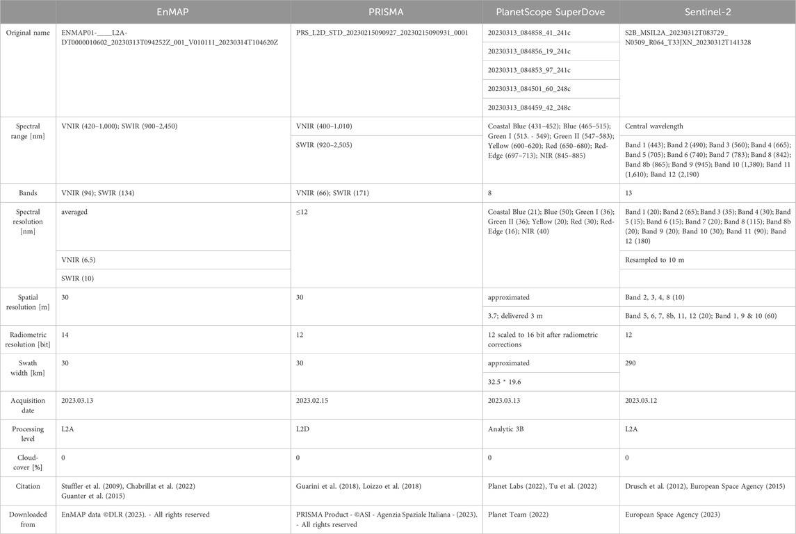
TABLE 1. Satellite image metadata.

2.3.3 Satellite data processing

The five images were processed identically using ENVI 5.5.3 software (L3Harris Geospatial Solutions, 2023). Images were clipped to the AOI extent and rescaled to values between 0 and 1. Endmember unmixing was performed using the Spectral Hourglass Wizard and the Minimum Noise Fraction (MNF) was applied to separate data from noise and to reduce data dimensionality (Green et al., 1988; Lee et al., 1990; Boardman and Kruse, 1994). The MNF transformation consists of two cascaded Principal Component Analysis rotations and a noise reduction step, and generally results in a better signal-to-noise ratio than simple Principal Component Analysis for noise reduction (Luo et al., 2016). The benefits of MNF for noise reduction in hyperspectral images are well known, but the analysis of multispectral data can also be improved (Syarif and Kumara, 2018). Figure 2 shows the MNF eigenvalue threshold used for each image and the remaining number of MNF bands where spatial coherence values are higher than the threshold. To estimate the abundance of an endmember in an image, several linear, nonlinear, and partial unmixing techniques have been tested in the last decades (Plaza et al., 2011; Quintano et al., 2012; Heylen et al., 2014; Wei and Wang, 2020; Peyghambari and Zhang, 2021; Cavalli, 2023). The advantage of partial unmixing methods such as Mixture Tuned Matched Filtering (MTMF) over other methods is that knowledge of background and other endmembers is not required to match individual endmembers, while the disadvantage is that this method is not suitable for mapping background (Boardman, 1998; Mundt et al., 2007; Boardman and Kruse, 2011). The MTMF process can be divided into two steps: The matched filter provides a score value representing the estimated abundance, and the mixture tuning provides an infeasibility value for each endmember and pixel (Boardman and Kruse, 2011). The infeasibility value indicates the quality of the matched filter result and allows detection of false positive pixels (Mundt et al., 2007). A pixel with a low score value should also have a low infeasibility value, while higher score values may be correct even if the infeasibility value is higher and score values above one mostly represent background (Mundt et al., 2007). Hence, the setting of infeasibility thresholds between correctly and falsely classified pixels is the most critical part of MTMF classification. Traditionally, this threshold is set manually using a 2D scatter plot of infeasibility and score values, followed by an iterative adjustment of the threshold using validation points (Boardman and Kruse, 2011). Alternatively, supervised learning algorithms or regression based thresholds can be used (Sankey, 2009; Routh et al., 2018). In this study, according to Kruse et al., 2015, a ratio of score to infeasibility value (ration = score value/infeasibility value) is used to standardize the results of the different satellite data and thus make them comparable. Only pixels with a ratio value greater than 0.025 were considered true, otherwise they were false positives. Additionally, all pixels with scores below 0.05 were considered false positives.

2.3.4 Validation approaches

Two approaches are used to validate unmixing results of all five datasets. The first approach is a linear regression between pixels classified as true by MTMF and the Normalized Difference Vegetation Index (NDVI), one of the most widely used vegetation indices in the world, and the Soil Adjusted Vegetation Index (SAVI), which is considered more sensitive in arid grasslands due to the canopy background adjustment factor (Rouse et al., 1974; Tucker, 1979; Huete, 1988; Zhou et al., 2014; Reinermann et al., 2020). This validation is based on the relationship between vegetation indices and increasing vegetation cover described by Purevdorj et al., 1998, and on the expected values of vegetation indices for arid vegetation and grass for both indices according to Huete, 1997. According to this study, the SAVI values for grass are around 0.2 to 0.4 and for semi-arid to arid vegetation below 0.2. For NDVI, the values for grass are around 0.3 to 0.6 and for semi-arid to arid vegetation below 0.5. The formulas for both indices are presented below:

$NDVI=\frac{NIR-Red}{NIR+Red};SAVI=\frac{1.5*\left(NIR-Red\right)}{\left(NIR+Red+0.5\right)}$

(Rouse et al., 1974; Tucker, 1979; Huete, 1988) Both indices were calculated from each dataset using the spectral indices tool in ENVI, where the bands selected for calculation are those closest to the center wavelength of 650 nm for Red and 860 nm for NIR. The indices are compared to MTMF results from same data set. The second validation attempt was carried out using the plots recorded during fieldwork. The 17 grass plots in the study area were compared to the correctly classified pixels of the MTMF. This allowed to determine how many of these plots were correctly classified. All graphs (Figures 3–13) were finally generated with the ggplot2 package using tidyverse, tidyterra and the terra package for remote sensing data in R (Hadley, 2016; Wickham et al., 2019; Hernangómez, 2023; Hijmans, 2023).

FIGURE 3

FIGURE 3. Fact sheet of measured soil spectra. (A) Example image of a measurement site on a grass plain and summarized information on all measured soil samples. (B) Spectral profiles using pistol measurements from all sites with mean spectra in yellow.

FIGURE 4

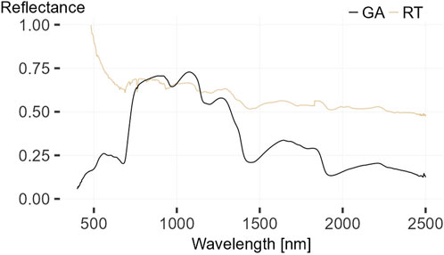
FIGURE 4. Contact spectra from Galenia africana (GA) and Rhigozum trichotomum (RT), whereas the measurement of Rhigozum trichotomum is not meaningful.

FIGURE 5

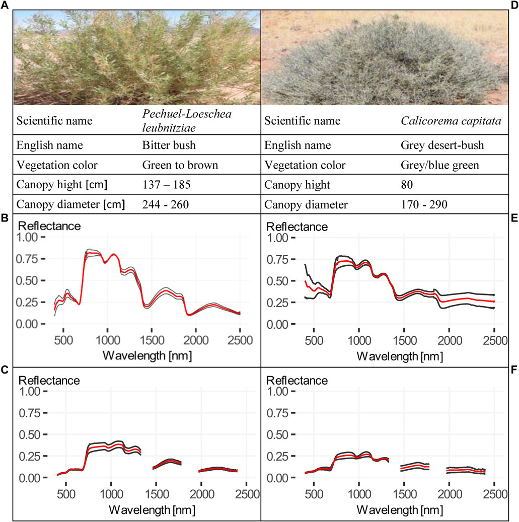
FIGURE 5. Fact sheets of Pechuel-Loeschea leubnitziae and Calicorema capitata. (A–C) Fact sheet of Pechuel-Loeschea leubnitziae, including (A) image and summarized information, (B) contact measurements and (C) pistol measurements. (D–F) Fact sheet of Calicorema capitata, including (D) image and summarized information, (E) contact measurements and (F) pistol measurements. All mean spectra in (B, C, E, F) are presented in red.

FIGURE 6

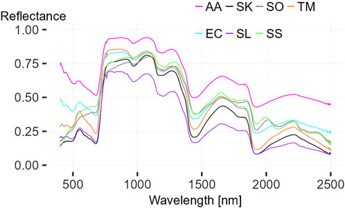
FIGURE 6. Contact measurement of Aristida adscensionis (AA), Enneapogon cenchroides (EC), Schmidtia kalihariensis (SK), Stipagrostis lutescens (SL), Stipagrostis obtusa (SO), Stipagrostis sabulicola (SS) and Tricholaena monachne (TM).

FIGURE 7

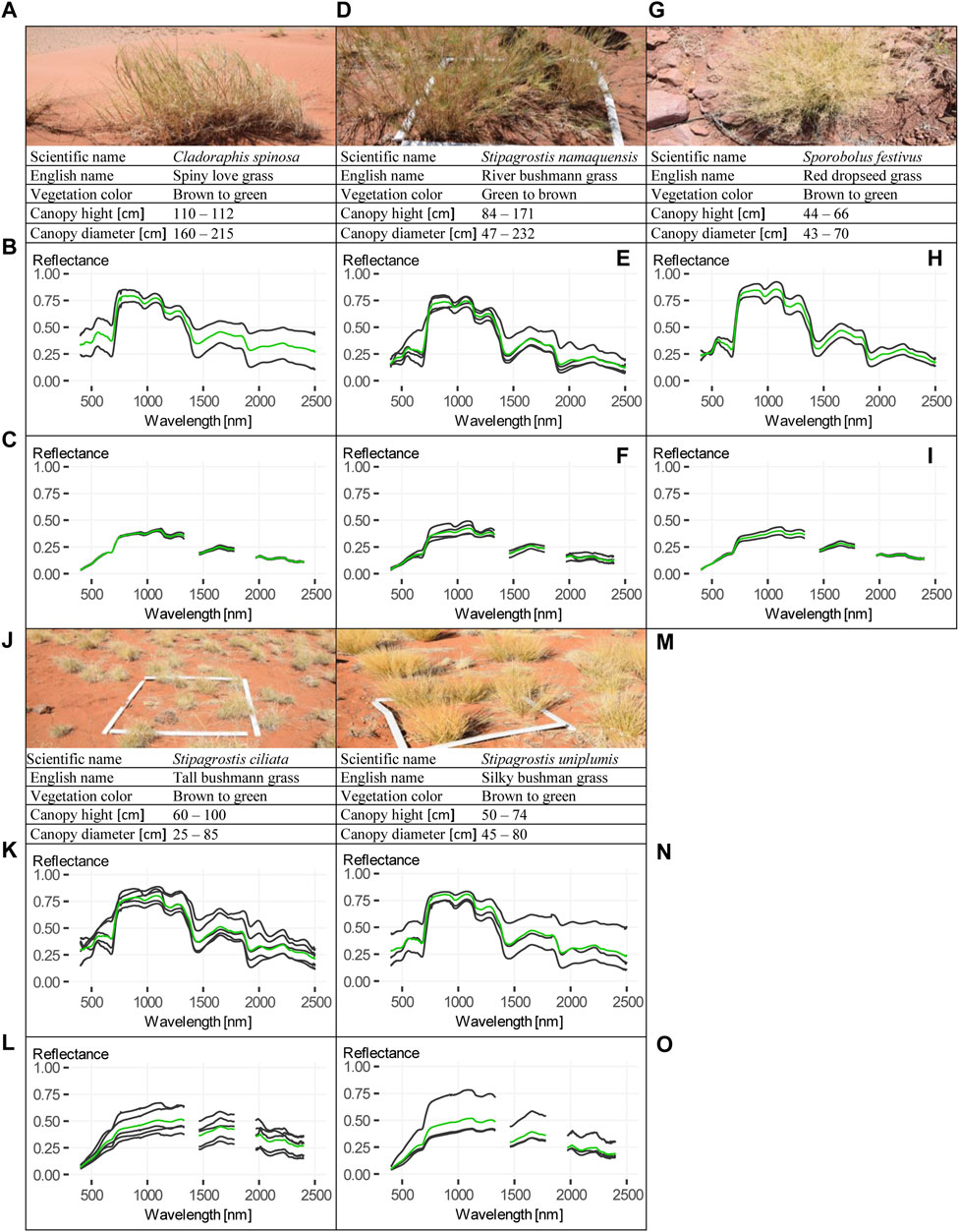
FIGURE 7. Fact sheets of Cladoraphis spinosa, Stipagrostis namaquensis, Sporobolus festivus, Stipagrostis ciliata and Stipagrostis uniplumis. (A–C) Fact sheet of Cladoraphis spinosa, including (A) image and summarized information, (B) contact measurements and (C) pistol measurements. (D–F) Fact sheet of Stipagrostis namaquensis, including (D) image and summarized information, (E) contact measurements and (F) pistol measurement. (G–I) Fact sheet of Sporobolus festivus, including (G) image and summarized information, (H) contact measurements and (I) pistol measurements. (J–L) Fact sheet of Stipagrostis ciliata, including (J) image and summarized information, (K) contact measurements and (L) pistol measurements. (M–O) Fact sheet of Stipagrostis uniplumis, including (M) image and summarized information, (N) contact measurements and (O) pistol measurements. All mean spectra in (B, C, E, F, H, I, K, L, N, O) are presented in green.

FIGURE 8

FIGURE 8. SAM analysis for all soil spectra with the mean soil spectra. Location of the plots: S01 hilly stony; S02 and S10 dune; S03, S04, S05, S06, S07 and S11 grass plain; S08, S09, S12 and S13 riverbed; SOIL mean soil spectra. See Supplementary Table S2 for exact values.

FIGURE 9

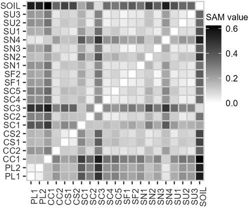
FIGURE 9. SAM analysis for vegetation spectra and comparison with the mean soil spectra. Abbreviations: PL Pechuel-Loeschea leubnitziae; CC Calicorema capitata; CS Cladoraphis spinosa; SC Stipagrostis ciliata; SF Sporobolus festivus; SN Stipagrostis namaquensis; SU Stipagrostis uniplumis; SOIL mean soil spectra. See Supplementary Table S3 for exact values and Supplementary Table S4 for mean SAM values for each species.

FIGURE 10

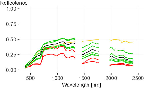
FIGURE 10. Endmember for MTMF. Mean spectra for both shrub spectra in red, all five grass mean spectra in green, soil mean spectra in yellow and the grass Endmember in black.

FIGURE 11

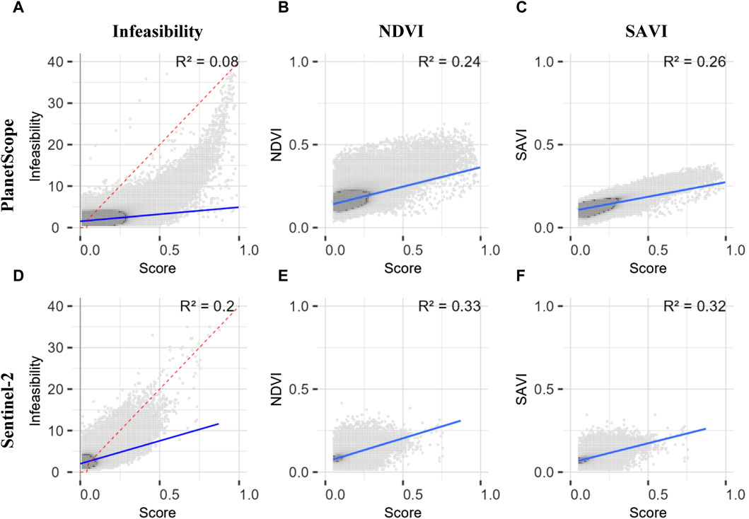
FIGURE 11. Scatterplots between infeasibility value, NDVI, SAVI and the score value for both multispectral images: PlanetScope and Sentinel-2. (A–F) show all aggregated pixels as a function of the number of pixels per value range. Darker areas represent more pixels than lighter areas. The regression line between both parameters is shown in blue and the R²-value is in the top right. Figure (A, D) show the scatterplot between infeasibility and score value with the threshold line in dashed red (Formula: y = x*0.025). In general, pixels with a score value below 0.05 are also classified as false positive. Figure (B, E) showing the scatterplot between NDVI and score value and Figure (C, F) between SAVI and score value. The score values represented in these figures compared to NDVI or SAVI are all pixels with a ratio >0.025 and a score value above 0.05. Maps of SAVI and NDVI for each image used for these plots are shown in Supplementary Figures S2A, B and Supplementary Figures S3A, B. In addition, identical scatterplots are shown in Supplementary Figure S4 for the results with a ratio threshold of 0.02, resulting in slightly lower R²-values for each regression.

FIGURE 12

FIGURE 12. Scatterplots between infeasibility value, NDVI, SAVI and the score value for both hyperspectral and data fusion images: PRISMA, EnMAP and SFIM-HS. Figures (A–I) show all aggregated pixels as a function of the number of pixels per value range. Darker areas represent more pixels than lighter areas. The regression line between both parameters is shown in blue and the R²-value is in the top right. Figure (A, D, G) show the scatterplot between infeasibility and score value with the threshold line in dashed red (Formula: y = x*0.025). In general, pixels with a score value below 0.05 are also classified as false positive. Figure (A, E, H) showing the scatterplot between NDVI and score value and Figure (A, F, I) between SAVI and score value. The score values represented in these figures compared to NDVI or SAVI are all pixels with a ratio >0.025 and a score value above 0.05. Maps of SAVI and NDVI for each image used for these plots are shown in Supplementary Figures S2C–E and Supplementary Figures S3C–E. In addition, identical scatterplots are shown in Supplementary Figure S5 for the results with a ratio threshold of 0.02, resulting in slightly lower R²-values for each regression.

FIGURE 13

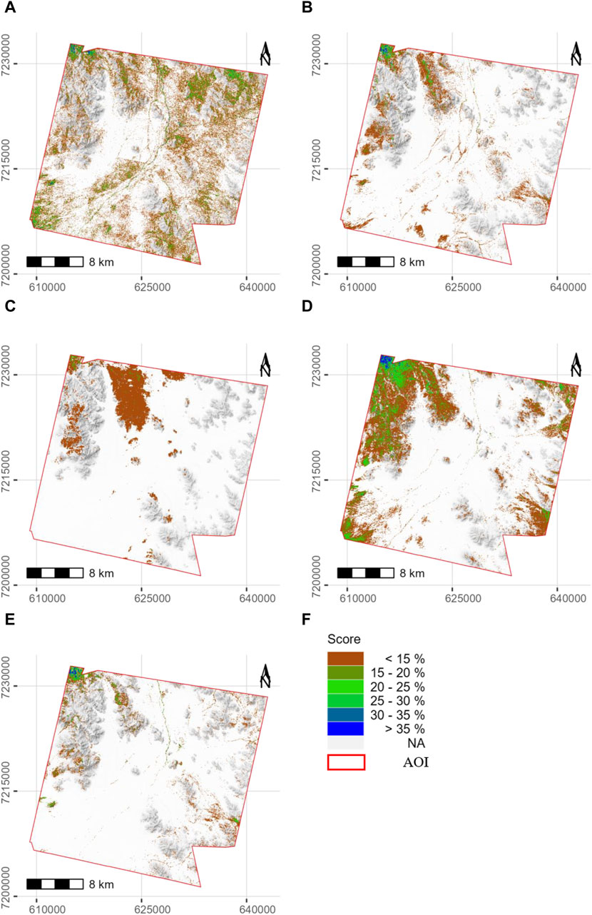
FIGURE 13. Distribution maps of grass endmember abundance. (A) PlanetScope, (B) Sentinel-2, (C) PRISMA, (D) EnMAP, (E) SFIM-HS, and (F) is showing the legend for all maps. The background map is a greyscale hill shade derived from TanDEM-X data (Resolution 12 m) (German Aerospace Center, 2022) using QGIS 3.28 Firenze (QGIS Development Team, 2023). Supplementary Figure S6 shows the comparative maps for a ratio threshold of 0.02. The distribution of grasses varies only slightly.

3 Results

This chapter presents and describes the measured soil, shrub, and grass spectra that form the first set of spectra in the unique spectral library. Intra-species spectral homogeneity, inter-species spectral separability, vegetation-soil separability, and soil homogeneity are derived from the SAM results to identify a likely endmember for grass unmixing under arid conditions. Finally, the resulting distribution maps of grass endmember abundance are described and validated.

3.1 Soil spectra

Thirteen soil spectra were collected during the field campaign, taken from vegetation-free grass plain, riverbed, and dune areas (Figure 3A). The collected soil samples showed nearly homogeneous color variation between dusky red, dark red, and dark reddish-brown (Figure 3A). Most of the samples had a clay content of about 20%, whereas one plot had a clay content of over 35%. Differences in grain size were found from the predominantly sandy loam, to sandy clay loam, to soils with more soil skeleton on the mountain slopes. Figure 3B) shows the spectra for each soil plot, highlighting the calculated mean soil spectrum in yellow. The soil spectra exhibit varying reflectance intensity across the spectrum. In addition, most spectra display a concave feature at 2,250 nm that varies in intensity and is absent in one spectrum.

3.2 Shrub spectra

Six shrub spectra from four different species could be measured during field work. Two species R. trichotomum, also known as Dreidorn, and Galenia africana, also known as Kraalbos, were measured only once and are not further illustrated, but the contact spectra are shown in Figure 4. Rhigozum trichotomum belongs to the family of Bignoniaceae and Galenia africana to the family of Aizoaceae. Due to the very dry and hard branches and the interfering thorns, the contact measurement of R. trichotomum was not meaningful. The Galenia africana was vigorous at the time of recording with partially browned leaves. However, the concave shape in the spectral range from 950 to 970 indicates a higher leaf water potential and thus lower water stress, probably due to the greener leaves measured (Figure 4). In addition, the two species Pechuel-Loeschea leubnitziae and C. capitata were measured twice at different locations (see fact sheet in Figure 5). Pechuel-Loeschea leubnitziae belongs to the family of Asteraceae. These measured shrubs were predominantly green, over 1 m high, over 2 m in diameter and were found in dry riverbeds in the study area. However, one was browner and is shown in Figure 5A). Calicorema capitata is a member of the Amaranthaceae family and has a greyish/bluish to green color and is shown in Figure 5D). They were found clustered on both large grassy plains and hilly regions with rocky substrates. Those that were measured were less than 1 m tall and had a diameter ranging from less than 2 m to nearly 3 m. The contact measurements of both species are shown in Figures 5B, E) and the pistol measurement in C) and F). All four figures contain a mean spectrum of the respective measurement type in red. The decrease of the spectral reflectance of one of the C. capitata spectra in the region below 500 nm indicates an interfering light incidence during the measurement. Otherwise, the region influenced by chlorophyll absorption and reflectance is less pronounced in the C. capitata spectra than in the Pechuel-Loeschea leubnitziae spectra. The cell wall absorption region indicates lower water stress for both species and the Pechuel-Loeschea leubnitziae spectrum shows more pronounced regions of higher reflectance in the biochemical region. The pistol measurement spectra were generally less informative for both species. For example, the region influenced by chlorophyll content is significantly less pronounced, similar to the region of cell water absorption. The Pechuel-Loeschea leubnitziae and the C. capitata are both frequently found in the study area, but are not dominant.

3.3 Grass spectra

A total of 23 spectra from 12 different Poaceae or grass species were measured during field work. Seven of them were measured once. The spectra from contact measurements are shown in Figure 6. The two grasses found on the dunes are Stipagrostis sabulicola also known as dune bushman-grass, which was measured on the top, and Stipagrostis lutescens, also commonly known as golden bushman-grass which was measured on the slope. Both dune grasses were more than one up to 2 m high. The comparison of both spectra shows lower chlorophyll and cell water absorption, indicating more water stress of S. sabulicola spectrum compared to S. lutescens spectrum. Tricholaena monachne, also known as blue-seed grass, Aristida adscensionis, also known as annual bristle grass, and Enneapogon cenchroides, also known as fur grass, were found together with S. uniplumis, Sporobolus festivus (both shown in Figure 7) and other non-presented species at the edge of a riverbed, the most species-rich area within this study site. The three species have similar spectra with different reflectance intensities, with the strong water absorption of the T. monachne spectrum showing a major a difference. In addition, the measurements of A. adscensionis and E. cenchroides in the region below 500 nm were partially disturbed by light incidence. On the plot where soil had a particularly high clay content (>35%), quite green S. kalihariensis, also known as bushman grass, could be found. However, some of these S. kalihariensis were disturbed by livestock grazing, but the spectrum tends to represent a grass that is higher stress resistant. Stipagrostis obtusa, the small bushman´s grass, located on a grass plain, showed a very brown condition. The spectrum also showed lower chlorophyll and cell water uptake, indicating water stress. Other species were measured more frequently and were therefore considered for further analysis (see fact sheets in Figure 7). One of these grasses is Cladoraphis spinosa, which was found and measured on top of a dune and on a sandy grass plain. The two specimens measured were almost the same height and in a rather brown condition. In dry riverbeds Stipagrostis namaquensis was more common. It was measured four times showing different conditions, from less than 1 m height and green to more than one and a half meter height and brown. Canopy diameter was very variable from less than 50 cm to almost 250 cm. Two Sporobolus festivus were found close to each other in the most species-rich area and did not differ much concerning phenological condition or size range. Two grass species clearly dominated within this study area. These were S. ciliata and S. uniplumis. Stipagrostis uniplumis was slightly shorter than S. ciliata, but both were less than a meter high. They were measured in either slightly greener or predominantly browner phenological states. Both species were found solitary or mixed, often occurring on grass plains or dry riverbeds. In general, the spectra of these five species show similarities across the spectrum, with S. ciliata having lower reflectance maxima in the 1,300–2,500 nm spectral range than other grasses. These grass spectra show lower chlorophyll and cell water absorption compared to shrub spectra, indicating increased water stress. Two spectra of S. ciliata and one spectrum of S. namaquensis stand out, showing particularly high reflectance in these spectral regions, indicating very dry conditions (Figures 7E, K). In the following, the intra-species spectral homogeneity, inter-species spectral separability, vegetation-soil separability and soil homogeneity of the spectra presented are described in more detail.

3.4 SAM analysis and derivation of endmember

The results of spectral separability analysis performed with SAM are shown in Figures 8, 9. They show the spectral angle between all soil spectra (Figure 8) and all vegetation spectra except species only measured once (Figure 9). The mean soil spectrum is also shown in both figures. Based on these results, intra-species spectral homogeneity, inter-species spectral separability, as well as separability from soil spectra, can be determined. The spectral angle between all soil spectra is very small, indicating high homogeneity. The calculated spectral angles range from 0.01 to 0.07. The two most similar spectra were measured on dunes. Largest difference is between one of these dune spectra and a spectrum taken from a stonier soil. The spectral angle between all soil spectra and mean soil spectra is less than 0.04, indicating the representativeness of mean spectra. Due to arid conditions in the study area, the soil spectra were considered as a background spectrum for partial unmixing. Therefore, the separability of vegetation from soil spectrum is important for successful unmixing. In general, the spectral angle between vegetation spectra and mean soil spectra is at least 0.30, indicating separability. Two exceptions are the spectra of very dry S. ciliata which show an angle of up to 0.08 (Figure 9). The spectra of Pechuel-Loeschea leubnitziae show the best separation from the mean soil spectrum, with high intra-species spectral homogeneity. While the intra-species spectral homogeneity of the shrub C. capitata is low with 0.28. Similarly, the inter-species spectral separability of C. capitata from spectra of the considered grass species and Pechuel-Loeschea leubnitziae is low, so separability cannot be granted. The comparison of SAM results of grass species in general shows that spectra of C. spinosa, S. uniplumis and Sporobolus festivus show a higher intra-species spectral homogeneity with a SAM angle below 0.06. In comparison, the spectra of S. ciliata and S. namaquensis show a lower intra-species spectral homogeneity depending on the condition of the measured grass. Occasionally, grass species show a higher inter-species spectral separability with a mean SAM angle greater than 0.1, with individual spectra being considerably smaller. For example, the spectra of C. spinosa and Sporobulus festivus show a high separability. However, the inter-species spectral separability of presented grass spectra is generally low, due to the extreme arid conditions during measurement. Therefore, individual grass species cannot be represented by the partial unmixing method. However, the SAM results show that it is possible to separate most of the grass spectra from soil spectra and the spectra of the shrub Pechuel-Loeschea leubnitziae. Therefore, a mean spectrum of all grass spectra was used as an endmember for partial unmixing. To improve this endmember, three spectra showing high similarity to soil or Pechuel-Loeschea leubnitziae spectra were excluded. The three excluded spectra are two from S. ciliata and one from S. namaquensis, labelled SC1, SC3 and SN4 in Figure 9. The calculated mean endmember for grass spectra is shown in Figure 10 along with the mean spectra of all species and soil.

3.5 Unmixing and validation

Before comparing the results from unmixing with the five different image datasets, it should be noted that the PRISMA image was taken in February, not at the time of fieldwork, which limits the comparability of PRISMA with the other four images. The results from MTMF and possible validation are presented in Table 2 and Figures 11–13. The scatterplots in Figures 11, 12 show aggregated pixels. Darker areas represent more pixels than brighter areas. Figures 11A, D show scatterplots between score and infeasibility values for all pixels with a score value between 0 and 1 and an infeasibility value between 0 and 40. The regression line is shown in blue, and the R-squared values for each image are low, up to 0.2. Pixels below the dashed red threshold line are classified as correct, while pixels above the line are classified as false positives and are not further considered. Score values decrease from nearly 1 for the high-resolution PlanetScope image to 0.7 for EnMAP and 0.25 for PRISMA, both being lower-resolution hyperspectral images. The PRISMA results show the least scatter (Figure 12A), which makes interpretation of results difficult. The SFIM-HS result, on the other hand, shows the widest dispersion of all, especially in the range of low scores and high infeasibility values (Figure 12G). This may indicate that fusion of high spectral and spatial resolution data improves the detectability of false positive pixels. The PlanetScope and Sentinel-2 results tend to show an exponential increase in infeasibility with increasing score values. The grass distribution maps from the five different images are shown in Figure 13. PRISMA shows single patches of grass in the central grass plains, on the slopes of the central hills, especially on the north slope, and larger patches of grass in the hillier north-central, northwestern, and western parts of the study area (Figure 13C). Similar spatial patterns are detected by the other sensors, but with varying degrees of intensity and spatial coverage. In general, PlanetScope shows more grass areas and also higher abundances throughout the study area (Figure 13A). The same is true for EnMAP in the western areas, while the SFIM-HS image (Figure 13) detects less grass compared to the other images. The northwestern area has the highest abundance of grass in all five distribution maps. Excluding PRISMA, the largest differences are in the northeast and southeast of the study area, where EnMAP and PlanetScope detect grass in the valley areas, while Sentinel-2 and SFIM-HS detect less to no grass in these areas. In addition, the SFIM-HS detects less grass cover in the southwestern grass plains compared to the other three datasets. PlanetScope and Sentinel-2 results show more grass in the dry riverbeds in the central-northern to central-southern areas, while EnMAP and SFIM-HS only partially detect it. To validate the results, the score values classified as correct were compared to NDVI and SAVI values of these pixels. In general, the NDVI and SAVI values shown are within the expected range and can therefore be considered realistic for grassland. The R²-values for the linear regression with NDVI ranged from 0.23 to 0.51 and from 0.26 to 0.66 with SAVI. The scatter of the points around the regression line was less for SAVI than for NDVI. The PlanetScope and PRISMA results have the lowest R² values. The results for Sentinel-2 and EnMAP are slightly better, with R²-values between 0.32 and 0.34 for both comparisons. Only the SFIM-HS results show higher R²-values of 0.51 for NDVI and 0.66 for SAVI. A second way of validation is to look at the 17 one-square meter grass plots within the study area. These plots, measured during the field work, were compared with to distribution maps from each image. The results are shown in Table 2. PRISMA detected only one grass plot. The results of the other four datasets are quite similar: only four of the grass plots were correctly identified by SFIM-HS, while the PlanetScope, Sentinel-2, and EnMAP images correctly identified six grass plots.

TABLE 2

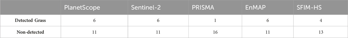
TABLE 2. Attempt to validate with the collected plots. Total number of grass plots: 17. A comparison table for the results with a ratio threshold of 0.02 is shown in Supplementary Table S5. With this threshold, the SFIM-HS image detects three more grass plots and PRISMA one more. Other results remain the same.

4 Discussion

In this chapter, the initial section examines field observations and the spectral library in regards to the current state of research and potential future developments. The subsequent section contextualizes the results of the sensor comparison, identifies limitations, and adjustments for enhancing the methodology for mapping grassland distribution. Finally, the discussions have yielded recommendations for future grassland monitoring in the NRNR and PNNR reserves, as well as for Greater Sossusvlei-Namib Landscape.

4.1 Field observations and spectral library

The field observations conducted in March 2023 reveal noteworthy contrasts in species distribution when compared to the Burke, 2022 survey. These distinctions are linked to significantly greater fluctuations in precipitation between the two rainy seasons of 2022 and 2023. Annual grasses such as S. kalihariensis, which was one of the dominant grass species in 2022, was almost absent in 2023. The only exception is the plot having a higher clay content and therefore a higher water capacity. Stipagrostis obtusa was also much less dominant in 2023 than in the previous year. The very common herb Gisekia africana could not be found at all in 2023. On the other hand, Sporobolus festivus, a grass not found in 2022, was found and measured this year. This grass is generally found in tropical Africa and northern Namibia, but also grows in poorly drained and rocky areas (van Oudtshoorn, 2022). The plot where Sporobolus festivus was found may have fulfilled the latter conditions. The only dominant grasses found in a similar distribution in both years, were S. ciliata and S. uniplumis. Stipagrostis namaquensis, the dominant grass in the dry riverbeds, was also common in 2023. The three dune grasses C. spinosa, S. lutescens and S. sabulicola were also found and measured in 2023. This comparison indicates that composition and biodiversity can vary greatly from year to year, and that the distribution of annual grasses in particular, but also of perennial grasses, is strongly dependent on precipitation. In future, it may be appropriate to monitor some of the species presented more closely, such as S. kalihariensis, which van Oudtshoorn, 2022 considered to be an important pioneer grass and a potential indicator of overgrazing, and whose distribution varied greatly from 2022 to 2023. The distribution of R. trichotomum, considered an invader, should also be monitored in the two reserves as well as in central and southern Namibia to mitigate possible bush encroachment (Shikangalah and Mapani, 2020; Burke, 2022). The distribution of Galenia africana deserves further analysis because of its medicinal value, for example, against breast cancer cells (Mohamed et al., 2020). Finally, it is necessary to conduct further research on the three dominant and drought-resistant grasses S. ciliata, S. uniplumis and S. namaquensis. These grasses play a vital role in the environment as they provide forage and protect the soil (van Oudtshoorn, 2022). The described field spectra of soils, shrubs and grasses, which form the basis of a unique spectral library of the arid grasslands of the Greater Sossusvlei-Namib Landscape, are invaluable for further research. Not only because the construction of this spectral library will begin to fill the knowledge gap of spectral information described by Jetz et al., 2016, but also because it may help to provide more information on forage quality and biodiversity, possible spread of invasive species and overgrazing in future (Ferner et al., 2015; Cavender-Bares et al., 2017). The spectral library presented here contains, as far as known, the first published spectra of the shrub species Pechuel-Loeschea leubnitziae and C. capitata and the grass species A. adscensionis, E. cenchroides, S. kalihariensis, S. lutescens, S. sabulicola, T. monachne and S. uniplumis. The spectra of S. obtusa, S. namaquensis, S. ciliata and of the shrub Galenia africana are included in the Frye et al., 2021 spectral library, but only in the 450–949 nm range, whereas all spectra presented here cover the 450–2,500 nm range, covering almost the entire range of characteristic absorption features of vegetation spectra (Kokaly et al., 2009; Ustin et al., 2009; Homolová et al., 2013). However, these spectra should only be considered as snapshots under very dry conditions. In order for this spectral library to have future application potential outside of this limited study area and to allow for longer term monitoring, the spectra should cover the phenological cycle of the recorded species (Somers et al., 2011; Dudley et al., 2015; Cavender-Bares et al., 2017). In addition, information on leaf photosynthetic pigments, leaf structure and biochemicals recorded in the field could help to better understand the variability of the spectra of individual species, but also between species, thus improving the applicability of the spectral library (Ollinger, 2011). The intra-species spectral homogeneity, inter-species spectral separability and separability from soil spectra, was determined using SAM. In general, the results show that grass spectra are separable from Pechuel-Loeschea leubnitziae spectra and soil spectra, whereas C. capitata spectra were too heterogeneous to clearly separate them from grass spectra. Intra-species spectra homogeneity of C. spinosa, S. uniplumis and Sporobolus festivus is particularly high, in contrast to S. ciliata and S. namaquensis. Some inter-species spectral separability could be observed, even though grasses showed different phenological stages depending on their location under extremely dry conditions in 2023. These conditions lead to less meaningful vegetation spectra, making it difficult to separate species. This fact can be confirmed in this study and was already described by Okin et al., 2001. As a consequence, the results of unmixing algorithms using satellite imagery worsen, leading to over-interpretation of vegetation cover (Okin et al., 2001). In addition, van Leeuwen et al., 2021 describe that species identification becomes more complex as spatial resolution decreases and biodiversity increases. For these reasons, it was decided not to attempt to map individual species in this study, but grass coverage in total. Identifying diagnostic wavelength ranges in which species are particularly separable could improve future attempts to map individual species. It is likely that these vary according to the influences described by Ollinger, 2011 and depend on phenology, but this identification needs further investigation.

4.2 Satellite data comparison and grassland distribution

This paper presents a suitable and unique approach to combine multi-sensor remote sensing data with collected field spectra to map grasslands within the Greater Sossusvlei-Namib Landscape and to identify limitations and advantages of each image data set. The approach used hyperspectral EnMAP and PRISMA data, multispectral Sentinel-2, PlanetScope and a SFIM-HS fused product. The results presented contribute to the research gap identified by Ferner et al., 2021 on whether multispectral or hyperspectral data are more effective for grassland monitoring, especially in arid regions. In addition, SFIM-HS images were compared to validate the assertion of Ghamisi et al., 2019 that data fusion improves target identification. The resulting grass distribution maps show clear differences, but also similarities. Grasses are detected particularly in the hilly northwest, where the highest abundances were recorded, as well as in the hilly regions of the north-central and western parts of the study area. Burke, 2022 also identified abundant grasses and shrubs in these areas in 2022, attributing this to cooler temperatures and increased precipitation due to elevation and the described west-east precipitation gradient of the study area. Terrain was not a central component of this study, but has high relevance as topo-edaphic conditions largely influence grassland vitality. The influence of terrain and seasonality on grassland dynamics and species composition has already been described by Masenyama et al., 2022; Dao et al., 2021; Reinermann et al., 2020 also describe the advantages of seasonal monitoring of grasslands, which is still rather limited due to the on-demand acquisition of hyperspectral imagery. As such, no PRISMA image could be acquired at the time of field work according to bad weather conditions, and thus a less comparable image from February 2023 was used. In combination with the described geolocation error of PRISMA and the necessary co-registration, which inevitably changed the reflectivity values slightly during resampling, the results using PRISMA imagery are of limited value and less comparable. However, the results of the NDVI and SAVI validation of the high spatial resolution PlanetScope image show similarly low R²-values. It can be assumed that PlanetScope overestimates grassland despite having the highest spatial resolution. According to Ali et al., 2016, the reason for this could be the low spectral coverage of 421–885 nm, leading to degraded target identification. The results of EnMAP and Sentinel-2 show almost identical R²-values despite considerable differences in the grassland distribution maps, especially in the hillier areas. The alleged over-interpretation of grass cover in the hilly areas of the EnMAP results is probably due to the low spatial resolution and small-scale relief in this area. The SFIM-HS product has higher R²-values of 0.55 (NDVI) and 0.66 (SAVI) and shows a distribution map that does not directly indicate overinterpretation. This supports the suggestion of Ghamisi et al., 2019 that data fusion improves target identification. However, the approach presented here has limitations as the distribution maps are based on a single mean grass endmember. The envisaged future use of phenological spectra will likely improve the spectral separability of species, allowing a Multi-Endmember Spectral Mixture Analysis, which can more adequately account for the spectral variability of individual species (Borsoi et al., 2021; Blanco et al., 2014 already combined the partial unmixing method MTMF used in this work with such a multi-endmember approach. Another limitation is the definition of threshold being the most arbitrary and influential part of MTMF. Here, a ratio threshold according to Kruse et al., 2015 was used to standardize and better compare the results of different datasets. According to Routh et al., 2018, supervised learning algorithms and cross-validation could be used to determine the “correct” threshold if enough good validation points are available. However, the one square meter plots used in this study are not sufficient for such an approach. Also, validation using these plots does not provide robust information on the quality of distribution maps, so larger validation plots are needed for future work, as already described by Sankey, 2009; Routh et al., 2018.

4.3 Outlook

Future research on dynamics of arid grasslands in both NRNR and PNNR, and in the wider context of grasslands in the Greater Sossusvlei-Namib Landscape, should adopt a more holistic spatio-temporal monitoring approach. This should include the Zhao et al., 2020 framework of pressure, state, response and a multi-scale, multi-method and multi-perspective approach. In order to fill the research gap on arid grasslands in southern Africa described by Van Cleemput et al., 2018; Reinermann et al., 2020; Masenyama et al., 2022 some adjustments need to be made. Although the AOI used in this study includes both reserves and adjacent farmland, no comparison between usage and management forms has been conducted. To further analyze the impact of human activities, a comparison is crucial. Hence, it would be advisable to expand the study area beyond the reserves to include monitoring of all adjacent commercial farmlands. This adaptation could provide valuable insights into the effects of different management strategies and the planned expansion of the PNNR. Additionally, it could enhance our comprehension of the dynamics along the rainfall gradient. Combining these two aspects may result in a greater understanding of the grassland ecosystem in the Greater Sossusvlei-Namib Landscape. The results presented in this paper show that neither multispectral nor hyperspectral data are better suited for monitoring grassland dynamics, but the results of the SFIM-HS product provide promising results. Further monitoring should therefore continue to use the three different types of data. The results also showed that the terrain affects the distribution of grasses, which should be further investigated. A TanDEM-X data set with a resolution of 12 m is already available for this purpose (German Aerospace Center, 2022). In future, distribution analysis of certain species such as R. trichotomum for monitoring potential bush encroachment, S. kalihariensis as a potential indicator of overgrazing, and the distribution of the dominant grasses S. ciliata, S. uniplumis and S. namaquensis due to their important functions in the environment is of high interest. The variable grassland species composition, as a result of precipitation intensity and distribution during the rainy season, indicates that additional species and compositions can be expected. Therefore, the unique spectral library presented here should be expanded and supplemented with additional information. This extension includes the measurement of phenological spectra and the determination of selected leaf photosynthetic pigments, leaf structure and biochemicals by laboratory and field measurements. This will help to better describe the spectral variability of species and make the spectral library useful for research outside the study area, improve unmixing results using multi-endmember approaches, and provide information on forage quality and biodiversity of grasslands (Ollinger, 2011; Somers et al., 2011; Dudley et al., 2015; Ferner et al., 2015; Cavender-Bares et al., 2017; Imran et al., 2021; Rocchini et al., 2022). Due to Mendelsohn and Mendelsohn, 2022; Huo et al., 2023; Lian et al., 2023 lower rainfall is expected in the upcoming rainy season due to a future El Niño phenomenon in 2024. As a result, an irrigated phenological garden could be established in collaboration with both reserves to measure the predominant grass and shrub spectra. In addition, the importance of larger validation points to determine the quality of distribution maps and for a more robust definition of the MTMF threshold according to Routh et al., 2018 was described. For this purpose, an unmanned aerial vehicle (UAV) equipped with a hyperspectral camera will be used to acquire imagery within plots of significantly larger size, surpassing 30 × 30 m in spatial extent. This will allow validation of lower resolution satellite data against high resolution UAV data. A DJI Matrice M300 RTK (DJI, 2023., Nanshan, Shenzhen, China) UAV equipped with a Black Bird V2 camera (Haip solutions, 2023,. Hanover, Germany) is available for this purpose. According to Gamon et al., 2019 the use of UAV data provides a layer of spatial resolution between field spectroscopy and satellite data and thus, together with field and laboratory measurements, allows the validation of biomass, forage quality, biodiversity and species identification of grasslands at satellite level (Pölönen et al., 2013; Librán-Embid et al., 2020; Geipel et al., 2021; Huelsman et al., 2023). UAVs have already been deployed in Namibia by Amputu et al., 2023 for mapping rangeland conditions in drylands. Another advantage of flying selected plots with the UAVs would be to map taller shrubs and acacias, which are less common in the area but cannot easily be measured with field spectroradiometers.

5 Conclusion

Grasslands in general have been degrading over the last decades, especially on the African continent. To date, only a few studies have used remote sensing techniques and specifically imaging spectroscopy to study arid grasslands, particularly in Namibia. This may be attributed to the aridity and resulting variability in vegetation cover associated with changes in the intensity of the rainy season, affecting the meaningfulness of the field spectra. The objectives of this study have been set to partially fill this knowledge gap. For this purpose, the grasslands of the two reserves NRNR and PNNR at the edge of the Namib Sand See were mapped for the first time in a selected area including large parts of PNNR and surrounding commercial farmlands using a multi-sensor remote sensing approach. The results were compared, and a unique spectral library was created based on the collected field spectra. The presented approach utilizes the MTMF algorithm to integrate field spectra data with satellite data from various sources, including multispectral PlanetScope and Sentinel-2, hyperspectral EnMAP and PRISMA, and the SFIM-HS product originated from Sentinel-2 and EnMAP. The study results demonstrate that neither multispectral nor hyperspectral data yields superior results in accurately mapping grasslands. However, the outcomes derived from the SFIM-HS product indicate that data fusion is a more effective approach for this purpose. Due to minimal precipitation during the 2023 rainy season, the resultant less meaningful spectra preclude any satellite-level analyses aimed at isolating particular grass species. Nevertheless, the present spectral library contains the first published spectra of two shrub and seven grass species, representing a small but significant contribution to filling the knowledge gap of spectral information on arid grasslands of Namibia. In future research, these spectral libraries should be expanded to encompass phenological spectra, as well as information of leaf structure, leaf photosynthetic pigments, and biochemicals, for each species. It is planned to expand the validation plots, incorporate UAV flyovers equipped with a hyperspectral camera, and carry out further analysis on the impact of terrain on grassland dynamics. Additionally, to expand the study area and further analyze the differences between commercial farmland and reserves. These adaptations could enable monitoring of the grasslands in the Greater Soussusvlei-Namib Landscape beyond the two reserves, allowing conclusions to be drawn about dynamics in biodiversity, forage quality, overgrazing, bush encroachment, desertification and implemented management strategies. Such adaptations could provide essential information for resident farmers and stakeholders to protect and better manage grasslands in future. This study adds to initial explorations of this unique ecosystem and contributes towards SDG 15 and the Decade of Restoration proclaimed by the United Nations.

Data availability statement

The original contributions presented in the study are included in the article/Supplementary Material, further inquiries can be directed to the corresponding author.

Author contributions

PB: Conceptualization, Formal Analysis, Methodology, Resources, Visualization, Writing–original draft, Writing–review and editing. DW: Conceptualization, Resources, Writing–review and editing. EP: Resources, Writing–review and editing. MK: Conceptualization, Resources, Writing–review and editing.

Funding

The author(s) declare that financial support was received for the research, authorship, and/or publication of this article. This research is the result of a self-financed project of the Department of Cartography, GIS and Remote Sensing for the preparation of a master’s thesis.

Acknowledgments

Many thanks to Jessica and André Steyn from NRNR and Murray and Lee Tindall from PNNR for the opportunity and support to conduct research in the two protected areas and to Albertine, Matin and Hange from NUST for their support during the field work.

Conflict of interest

The authors declare that the research was conducted in the absence of any commercial or financial relationships that could be construed as a potential conflict of interest.

Publisher’s note

All claims expressed in this article are solely those of the authors and do not necessarily represent those of their affiliated organizations, or those of the publisher, the editors and the reviewers. Any product that may be evaluated in this article, or claim that may be made by its manufacturer, is not guaranteed or endorsed by the publisher.

Supplementary material

The Supplementary Material for this article can be found online at: https://www.frontiersin.org/articles/10.3389/frsen.2024.1368551/full#supplementary-material

References

Acito, N., Diani, M., and Corsini, G. (2022). PRISMA spatial resolution enhancement by fusion with sentinel-2 data. IEEE J. Sel. Top. Appl. Earth Obs. Remote Sens. 15, 62–79. doi:10.1109/JSTARS.2021.3132135

CrossRef Full Text | Google Scholar

Ali, I., Cawkwell, F., Dwyer, E., Barrett, B., and Green, S. (2016). Satellite remote sensing of grasslands: from observation to management. JPECOL 9, 649–671. doi:10.1093/jpe/rtw005

CrossRef Full Text | Google Scholar

Amputu, A., Tielboerger, K., Knox, N., and Delaby, L. (2022). “Drone-based multispectral imagery is effective for determining forage availability in arid savannas,” in Grassland at the heart of circular and sustainable food systems: Proceedings of the 29th General Meeting of the European Grassland Federation : Caen, France, Paris, 26-30 June 2022 (INRAE), 527–529. The Organising Comittee of the 29th general meering of the European Grassland Federation.

Google Scholar

Amputu, V., Knox, N., Braun, A., Heshmati, S., Retzlaff, R., Röder, A., et al. (2023). Unmanned aerial systems accurately map rangeland condition indicators in a dryland savannah. Ecol. Inf. 75, 102007. doi:10.1016/j.ecoinf.2023.102007

CrossRef Full Text | Google Scholar

Analytical Spectral Devices Inc (2008a). RS3 user manual: ASD document 600545. USA: Rev. E. Boulder.

Google Scholar

Analytical Spectral Devices Inc (2008b). ViewSpec Pro user manual: ASD document 600555. Boulder, USA: Rev. A.

Google Scholar

Analytical Spectral Devices Inc (2010a). FieldSpec 3 user manual: ASD document 600540 rev. USA: J. Boulder.

Google Scholar

Analytical Spectral Devices Inc (2010b). ASD leaf Clip: model: a122317; SN: 129. USA: Boulder.

Google Scholar

Baiocchi, V., Giannone, F., and Monti, F. (2022). How to orient and orthorectify PRISMA images and related issues. Remote Sens. 14, 1991. doi:10.3390/rs14091991

CrossRef Full Text | Google Scholar

Bardgett, R. D., Bullock, J. M., Lavorel, S., Manning, P., Schaffner, U., Ostle, N., et al. (2021). Combatting global grassland degradation. Nat. Rev. Earth Environ. 2, 720–735. doi:10.1038/s43017-021-00207-2

CrossRef Full Text | Google Scholar

Beleites, C., and Sergo, V. (2021). HyperSpec: a package to handle hyperspectral data sets in R. package version 0.100.0.

Google Scholar

Bengtsson, J., Bullock, J. M., Egoh, B., Everson, C., Everson, T., O'Connor, T., et al. (2019). Grasslands-more important for ecosystem services than you might think. Ecosphere 10, e02582. doi:10.1002/ecs2.2582

CrossRef Full Text | Google Scholar

Blair, J., Nippert, J., and Briggs, J. (2014). “Grassland ecology,” in Ecology and the environment. Editor R. K. Monson (Dordrecht: Springer), 389–423.

CrossRef Full Text | Google Scholar

Blanco, P. D., Del Valle, H. F., Bouza, P. J., Metternicht, G. I., and Hardtke, L. A. (2014). Ecological site classification of semiarid rangelands: synergistic use of Landsat and Hyperion imagery. Int. J. Appl. Earth Observation Geoinformation 29, 11–21. doi:10.1016/j.jag.2013.12.011

CrossRef Full Text | Google Scholar

Boardman, J. W. (1998). Leveraging the high dimensionality of AVIRIS data for improved sub-pixel target unmixing and rejection of false positives: mixture Tuned Matched Filtering. Proc. 7th Annu. JPL Airborne Geoscience Workshop 55.

Google Scholar

Boardman, J. W., and Kruse, F. A. (1994). “Automated spectral analysis: a geological example using aviris data, north grapevine mountains, Nevada,” in Proc.10th Thematic Conference on Geological Remote Sensing, San Antonio, 407–418. ERIM.

Google Scholar

Boardman, J. W., and Kruse, F. A. (2011). Analysis of imaging spectrometer data using $N$-Dimensional geometry and a mixture-tuned matched filtering approach. IEEE Trans. Geosci. Remote Sens. 49, 4138–4152. doi:10.1109/TGRS.2011.2161585

CrossRef Full Text | Google Scholar

Borsoi, R. A., Imbiriba, T., Bermudez, J. C. M., Richard, C., Chanussot, J., Drumetz, L., et al. (2021). Spectral variability in hyperspectral data unmixing: a comprehensive review. IEEE Geosci. Remote Sens. Mag. 9, 223–270. doi:10.1109/MGRS.2021.3071158

CrossRef Full Text | Google Scholar

Burke, A. (2008). Pflanzenführer für die südliche Namib. Windhoek: Namibia Wissenschaftliche Gesellschaft; [Hess].

Google Scholar

Burke, A. (2009a). Wild flowers of the central Namib. Windhoek: Namibia Scientific Soc.

Google Scholar

Burke, A. (2009b). Wild flowers of the northern Namib. Windhoek: Namibia Scientific Society.

Google Scholar

Burke, A. (2022). Vegetation map for the NamibRand and ProNamib nature reserves. Report for NamibRand. Windhoek: Enviro Science.

Google Scholar

Cavalli, R. M. (2023). Spatial validation of spectral unmixing results: a systematic review. Remote Sens. 15, 2822. doi:10.3390/rs15112822

CrossRef Full Text | Google Scholar

Cavender-Bares, J., Gamon, J. A., Hobbie, S. E., Madritch, M. D., Meireles, J. E., Schweiger, A. K., et al. (2017). Harnessing plant spectra to integrate the biodiversity sciences across biological and spatial scales. Am. J. Bot. 104, 966–969. doi:10.3732/ajb.1700061

PubMed Abstract | CrossRef Full Text | Google Scholar

Chabrillat, S., Guanter, L., Kaufmann, H., Foerster, S., Beamish, A., Brosinsky, A., et al. (2022). EnMAP science plan. GFZ Data Services. doi:10.48440/enmap.2022.001

CrossRef Full Text | Google Scholar

Chan, J. C.-W., and Yokoya, N. (2016). “Mapping land covers of brussels capital region using spatially enhanced hyperspectral images,” in 2016 8th Workshop on Hyperspectral Image and Signal Processing: Evolution in Remote Sensing (WHISPERS IEEE), 1–5.

CrossRef Full Text | Google Scholar

Dao, P. D., Axiotis, A., and He, Y. (2021). Mapping native and invasive grassland species and characterizing topography-driven species dynamics using high spatial resolution hyperspectral imagery. Int. J. Appl. Earth Observation Geoinformation 104, 102542. doi:10.1016/j.jag.2021.102542

CrossRef Full Text | Google Scholar

Dennison, P., Daughtry, C., Quemada, M., Roth, K., Numata, I., Meerdink, S., et al. (2019a). Fractional cover simulated VSWIR dataset Version 2, noise and atmos. correction artifacts included. EcoSIS.

Google Scholar

Dennison, P., Daughtry, C., Quemada, M., Roth, K., Numata, I., Meerdink, S., et al. (2019b). Fractional cover simulated VSWIR dataset Version 2, original 10nm spectra. EcoSIS.

Google Scholar

Dennison, P. E., and Gardner, M. E. (2016). Hawaii 2000 vegetation species spectra. EcoSIS.

Google Scholar

Derner, J., and Schuman, G. (2007). Carbon sequestration and rangelands: a synthesis of land management and precipitation effects. J. soil water conservation, 77–85.

Google Scholar

Deshmukh, J. K. (1984). A common relationship between precipitation and grassland peak biomass for East and southern Africa. Afr. J. Ecol. 22, 181–186. doi:10.1111/j.1365-2028.1984.tb00693.x

CrossRef Full Text | Google Scholar

Dirkx, E., Hager, C., Tadross, M., Bethune, S., and Curtis, B. (2008). Climate change: vulnerability and adaptation assessment Namibia. Final Report.

Google Scholar

DJI (2023). Matrice 300 RTK - industrielle kartierungs-inspektionsdrohnen - DJI enterprise. https://enterprise.dji.com/de/matrice-300 (Accessed August 30, 2023).

Google Scholar

Drusch, M., Del Bello, U., Carlier, S., Colin, O., Fernandez, V., Gascon, F., et al. (2012). Sentinel-2: ESA's optical high-resolution mission for GMES operational services. Remote Sens. Environ. 120, 25–36. doi:10.1016/j.rse.2011.11.026

CrossRef Full Text | Google Scholar

Dudley, K. L., Dennison, P. E., Roth, K. L., Roberts, D. A., and Coates, A. R. (2015). A multi-temporal spectral library approach for mapping vegetation species across spatial and temporal phenological gradients. Remote Sens. Environ. 167, 121–134. doi:10.1016/j.rse.2015.05.004

CrossRef Full Text | Google Scholar

EnMAP-Box Developers (2019). EnMAP-Box 3 - a QGIS Plugin to process and visualize hyperspectral remote sensing data.Version 3.11.

Google Scholar

European Space Agency (2015). Sentinel-2 user handbook. https://sentinels.copernicus.eu/documents/247904/685211/Sentinel-2_User_Handbook.

Google Scholar

European Space Agency (2023). Copernicus open access hub. https://scihub.copernicus.eu/dhus/#/home.

Google Scholar

Ferner, J., Linstädter, A., Rogass, C., Südekum, K.-H., and Schmidtlein, S. (2021). Towards forage resource monitoring in subtropical savanna grasslands: going multispectral or hyperspectral? Eur. J. Remote Sens. 54, 364–384. doi:10.1080/22797254.2021.1934556

CrossRef Full Text | Google Scholar

Ferner, J., Linstädter, A., Südekum, K.-H., and Schmidtlein, S. (2015). Spectral indicators of forage quality in West Africa’s tropical savannas. Int. J. Appl. Earth Observation Geoinformation 41, 99–106. doi:10.1016/j.jag.2015.04.019

CrossRef Full Text | Google Scholar

Frye, H., Aeillo-Lammens, M. E., Euston-Brown, D., Jones, C. S., Kilroy Mollmann, H., Merow, C., et al. (2021). Greater cape floristic region leaf. Spectral Library. EcoSIS.

Google Scholar

Funk, C., Peterson, P., Landsfeld, M., Pedreros, D., Verdin, J., Shukla, S., et al. (2015). The climate hazards infrared precipitation with stations--a new environmental record for monitoring extremes. Sci. Data 2, 150066. doi:10.1038/sdata.2015.66

PubMed Abstract | CrossRef Full Text | Google Scholar

GADM (2022). Namibia grenzen (shapefile). https://gadm.org/download_country_v3.html (Accessed June 22, 2022).

Google Scholar

Gamon, J. A., Somers, B., Malenovský, Z., Middleton, E. M., Rascher, U., and Schaepman, M. E. (2019). Assessing vegetation function with imaging spectroscopy. Surv. Geophys 40, 489–513. doi:10.1007/s10712-019-09511-5

CrossRef Full Text | Google Scholar

Gang, C., Zhou, W., Chen, Y., Wang, Z., Sun, Z., Li, J., et al. (2014). Quantitative assessment of the contributions of climate change and human activities on global grassland degradation. Environ. Earth Sci. 72, 4273–4282. doi:10.1007/s12665-014-3322-6

CrossRef Full Text | Google Scholar

Garmin International Inc (2005). GPSMAP 60CSx.

Google Scholar

Geipel, J., Bakken, A. K., Jørgensen, M., and Korsaeth, A. (2021). Forage yield and quality estimation by means of UAV and hyperspectral imaging. Precis. Agric. 22, 1437–1463. doi:10.1007/s11119-021-09790-2

CrossRef Full Text | Google Scholar

Geofabrik, (2018). OpenStreetMap data of Namibia (shapefile). https://download.geofabrik.de/africa/namibia.html (Accessed June 22, 2022).

Google Scholar

German Aerospace Center (2022) TanDEM-X (12 m resolution) Products supplied under an DLR license for use. TDM.DEM.DEM/TDM1_DEM__04_S26E016_V01_C; TDM.DEM.DEM/TDM1_DEM__04_S26E015_V01_C; TDM.DEM.DEM/TDM1_DEM__04_S25E016_V01_C; TDM.DEM.DEM/TDM1_DEM__04_S25E015_V01_C; German Aerospace Center. Oberpfaffenhofen.

Google Scholar

German Aerospace Center (2023). EnMAP Products supplied under an DLR license for use. ENMAP01-____L2A-DT0000010602_20230313T094252Z_001_V010111_20230314T104620Z.

Google Scholar

Ghamisi, P., Gloaguen, R., Atkinson, P. M., Benediktsson, J. A., Rasti, B., Yokoya, N., et al. (2019). Multisource and multitemporal data fusion in remote sensing: a comprehensive review of the state of the art. IEEE Geosci. Remote Sens. Mag. 7, 6–39. doi:10.1109/MGRS.2018.2890023

CrossRef Full Text | Google Scholar

Gibson, D. J. (2009). Grasses and grassland ecology. Oxford: Oxford University Press.

Google Scholar

Goetz, A. F., Vane, G., Solomon, J. E., and Rock, B. N. (1985). Imaging spectrometry for Earth remote sensing. Science 228, 1147–1153. doi:10.1126/science.228.4704.1147

PubMed Abstract | CrossRef Full Text | Google Scholar

Gorelick, N., Hancher, M., Dixon, M., Ilyushchenko, S., Thau, D., and Moore, R. (2017). Google Earth engine: planetary-scale geospatial analysis for everyone. Remote Sens. Environ. 202, 18–27. doi:10.1016/j.rse.2017.06.031

CrossRef Full Text | Google Scholar

Green, A. A., Berman, M., Switzer, P., and Craig, M. D. (1988). A transformation for ordering multispectral data in terms of image quality with implications for noise removal. IEEE Trans. Geosci. Remote Sens. 26, 65–74. doi:10.1109/36.3001

CrossRef Full Text | Google Scholar

Guanter, L., Kaufmann, H., Segl, K., Foerster, S., Rogass, C., Chabrillat, S., et al. (2015). The EnMAP spaceborne imaging spectroscopy mission for Earth observation. Remote Sens. 7, 8830–8857. doi:10.3390/rs70708830

CrossRef Full Text | Google Scholar

Guarini, R., Loizzo, R., Facchinetti, C., Longo, F., Ponticelli, B., Faraci, M., et al. (2018). “Prisma hyperspectral mission products”. in IGARSS 2018 - 2018 IEEE International Geoscience and Remote Sensing Symposium. IEEE, 179–182.

CrossRef Full Text | Google Scholar

Hadley, W. (2016). ggplot2: elegant graphics for data analysis. New York: Springer-Verlag.

Google Scholar

Haip solutions (2023). BlackBird V2 │ hyperspectral camera drone │ plug and play for DJI drones. https://www.haip-solutions.com/hyperspectral-camera-drone/(Accessed August 30, 2023).

Google Scholar

Hernangómez, D. (2023). tidyterra: 'tidyverse' Methods and 'ggplot2' Helpers for 'terra' Objects. Zenodo. doi:10.5281/zenodo.7674165

CrossRef Full Text | Google Scholar

Heylen, R., Parente, M., and Gader, P. (2014). A review of nonlinear hyperspectral unmixing methods. IEEE J. Sel. Top. Appl. Earth Obs. Remote Sens. 7, 1844–1868. doi:10.1109/JSTARS.2014.2320576

CrossRef Full Text | Google Scholar

Hijmans, R. J. (2023). Terra: spatial data analysis: R package version 1, 7–29.

Google Scholar

Homolová, L., Malenovský, Z., Clevers, J. G., García-Santos, G., and Schaepman, M. E. (2013). Review of optical-based remote sensing for plant trait mapping. Ecol. Complex. 15, 1–16. doi:10.1016/j.ecocom.2013.06.003

CrossRef Full Text | Google Scholar

Huelsman, K., Epstein, H., Yang, X., Mullori, L., Červená, L., and Walker, R. (2023). Spectral variability in fine-scale drone-based imaging spectroscopy does not impede detection of target invasive plant species. Front. Remote Sens. 3. doi:10.3389/frsen.2022.1085808

CrossRef Full Text | Google Scholar

Huete, A. (1988). A soil-adjusted vegetation index (SAVI). Remote Sens. Environ. 25, 295–309. doi:10.1016/0034-4257(88)90106-X

CrossRef Full Text | Google Scholar

Huete, A. (1997). A comparison of vegetation indices over a global set of TM images for EOS-MODIS. Remote Sens. Environ. 59, 440–451. doi:10.1016/S0034-4257(96)00112-5

CrossRef Full Text | Google Scholar

Huo, W., Xiao, Z., Zhao, L., and Liu, F. (2023). Ascending phase of solar cycle 25 tilts the current El Niño–Southern Oscillation transition. Atmos. Ocean. Sci. Lett. 17, 100397. doi:10.1016/j.aosl.2023.100397

CrossRef Full Text | Google Scholar

Imran, H. A., Gianelle, D., Scotton, M., Rocchini, D., Dalponte, M., Macolino, S., et al. (2021). Potential and limitations of grasslands α-diversity prediction using fine-scale hyperspectral imagery. Remote Sens. 13, 2649. doi:10.3390/rs13142649

CrossRef Full Text | Google Scholar

International Union of Soil Sciences (2022). World Reference Base for Soil Resources. International soil classification system for naming soils and creating legends for soil maps. Vienna, Austria: International Union of Soil Sciences.

Google Scholar

Italian Space Agency (2023). Prisma Products supplied under an ASI license for use: prs_L2D_STD_20230215090927_20230215090931_0001.

Google Scholar

Jetz, W., Cavender-Bares, J., Pavlick, R., Schimel, D., Davis, F. W., Asner, G. P., et al. (2016). Monitoring plant functional diversity from space. Nat. Plants 2, 16024. doi:10.1038/nplants.2016.24

PubMed Abstract | CrossRef Full Text | Google Scholar

Jiménez, M., and Díaz-Delgado, R. (2015). Towards a standard plant species spectral library protocol for vegetation mapping: a case study in the shrubland of doñana national Park. IJGI 4, 2472–2495. doi:10.3390/ijgi4042472

CrossRef Full Text | Google Scholar

Jin, X. (2017). ENVI automated image registration solutions: whitepaper. https://www.l3harrisgeospatial.com/portals/0/pdfs/ENVI_Image_Registration_Whitepaper.pdf (Accessed May 23, 2023).

Google Scholar

Juergens, N., Oldeland, J., Hachfeld, B., Erb, E., and Schultz, C. (2013). Ecology and spatial patterns of large-scale vegetation units within the central Namib Desert. J. Arid Environ. 93, 59–79. doi:10.1016/j.jaridenv.2012.09.009

CrossRef Full Text | Google Scholar

Kalacska, M., Pablo Arroyo-Mora, J., Soffer, R., and Elmer, K. (2018). ASD FieldSpec3 field measurement protocols v1.

Google Scholar

Kleppel, G. S., and Frank, D. A. (2022). Structure and functioning of wild and agricultural grazing ecosystems: a comparative review. Front. Sustain. Food Syst. 6. doi:10.3389/fsufs.2022.945514

CrossRef Full Text | Google Scholar

Knox, N. M., Skidmore, A. K., Prins, H. H., Asner, G. P., van der Werff, H. M., Boer, W. F. de, et al. (2011). Dry season mapping of savanna forage quality, using the hyperspectral Carnegie Airborne Observatory sensor. Remote Sens. Environ. 115, 1478–1488. doi:10.1016/j.rse.2011.02.007

CrossRef Full Text | Google Scholar

Kokaly, R. F., Asner, G. P., Ollinger, S. V., Martin, M. E., and Wessman, C. A. (2009). Characterizing canopy biochemistry from imaging spectroscopy and its application to ecosystem studies. Remote Sens. Environ. 113, S78–S91. doi:10.1016/j.rse.2008.10.018

CrossRef Full Text | Google Scholar

Kokaly, R. F., Clark, R. N., Swayze, G. A., Livo, K. E., Hoefen, T. M., Pearson, N. C., et al. (2017). Data series. Data series. Reston, VA: US Geological Survey. doi:10.3133/ds1035

CrossRef Full Text | Google Scholar

Kose, M., Melts, I., and Heinsoo, K. (2022). Medicinal plants in semi-natural grasslands: impact of management. Plants (Basel) 11, 353. doi:10.3390/plants11030353

PubMed Abstract | CrossRef Full Text | Google Scholar

Kruse, F. A., Baugh, W. M., and Perry, S. L. (2015). Validation of DigitalGlobe WorldView-3 Earth imaging satellite shortwave infrared bands for mineral mapping. J. Appl. Remote Sens. 9, 096044. doi:10.1117/1.JRS.9.096044

CrossRef Full Text | Google Scholar

Kruse, F. A., Lefkoff, A. B., Boardman, J. W., Heidebrecht, K. B., Shapiro, A. T., Barloon, P. J., et al. (1993). The spectral image processing system (SIPS)—interactive visualization and analysis of imaging spectrometer data. Remote Sens. Environ. 44, 145–163. doi:10.1016/0034-4257(93)90013-N

CrossRef Full Text | Google Scholar

L3Harris Geospatial Solutions (2023). ENVI 5.5.3. Available at: https://www.l3harrisgeospatial.com/Support/Maintenance-Detail/ArtMID/13350/ArticleID/23834/ENVI-553-Release-Notes.

Google Scholar

Latham, J., Cumani, R., Rosati, I., and Bloise, M. (2014). Global land cover share (GL-SHARE): database beta-release version 1.0-2014. https://www.fao.org/uploads/media/glc-share-doc.pdf (Accessed May 20, 2023).

Google Scholar

Lee, J. B., Woodyatt, A. S., and Berman, M. (1990). Enhancement of high spectral resolution remote-sensing data by a noise-adjusted principal components transform. IEEE Trans. Geosci. Remote Sens. 28, 295–304. doi:10.1109/36.54356

CrossRef Full Text | Google Scholar

Lehnert, L. W., Meyer, H., Obermeier, W. A., Silva, B., Regeling, B., and Bendix, J. (2019). Hyperspectral data analysis in R: the hsdar package. J. Stat. Soft. 89. doi:10.18637/jss.v089.i12

CrossRef Full Text | Google Scholar

Leutner, B., Horning, N., and Schwalb-Willmann, J. (2023). RStoolbox: tools for remote sensing data analysis.

Google Scholar

Lian, T., Wang, J., Chen, D., Liu, T., and Wang, D. (2023). A strong 2023/24 El Niño is staged by tropical pacific ocean heat content buildup. Ocean-Land-Atmos Res. 2. doi:10.34133/olar.0011

CrossRef Full Text | Google Scholar

Librán-Embid, F., Klaus, F., Tscharntke, T., and Grass, I. (2020). Unmanned aerial vehicles for biodiversity-friendly agricultural landscapes - a systematic review. Sci. Total Environ. 732, 139204. doi:10.1016/j.scitotenv.2020.139204

PubMed Abstract | CrossRef Full Text | Google Scholar

Lieth, H. (1974). Phenology and seasonality modeling proc conf. Minneapolis aug 1972. New York: Chapman and Hall. Place of publication not identified.

Google Scholar

Liu, J. G. (2000). Smoothing Filter-based Intensity Modulation: a spectral preserve image fusion technique for improving spatial details. Int. J. Remote Sens. 21, 3461–3472. doi:10.1080/014311600750037499

CrossRef Full Text | Google Scholar

Liu, X., and Zhou, J. (2021). Assessment of the continuous extreme drought events in Namibia during the last decade. Water 13, 2942. doi:10.3390/w13202942

CrossRef Full Text | Google Scholar

Loizzo, R., Guarini, R., Longo, F., Scopa, T., Formaro, R., Facchinetti, C., et al. (2018). “Prisma: the Italian hyperspectral mission,” in IGARSS 2018 - 2018 IEEE International Geoscience and Remote Sensing Symposium (IEEE), 175–178.

CrossRef Full Text | Google Scholar

Luo, G., Chen, G., Tian, L., Qin, K., and Qian, S.-E. (2016). Minimum noise fraction versus principal component analysis as a preprocessing step for hyperspectral imagery denoising. Can. J. Remote Sens. 42, 106–116. doi:10.1080/07038992.2016.1160772

CrossRef Full Text | Google Scholar

MacDonald, J. S., Ustin, S. L., and Schaepman, M. E. (2009). The contributions of Dr. Alexander F.H. Goetz to imaging spectrometry. Remote Sens. Environ. 113, S2–S4. doi:10.1016/j.rse.2008.10.017

CrossRef Full Text | Google Scholar

Maestre, F. T., Le Bagousse-Pinguet, Y., Delgado-Baquerizo, M., Eldridge, D. J., Saiz, H., Berdugo, M., et al. (2022). Grazing and ecosystem service delivery in global drylands. Science 378, 915–920. doi:10.1126/science.abq4062

PubMed Abstract | CrossRef Full Text | Google Scholar

Männer, F., Dubrovyk, O., Ferner, J., Freyaldenhoven, A., Muro, J., Schmidtlein, S., et al. (2022). “Forage quality predicted by hyperspectral reflection measurements across climate zones,” in Grassland at the heart of circular and sustainable food systems: proceedings of the 29th general meeting of the European grassland federation: caen, France 26-30 june 2022. The organising comittee of the 29th general meering of the European grassland federation. Editor L. Delaby (Paris: INRAE), 656–658.

Google Scholar

Masenyama, A., Mutanga, O., Dube, T., Bangira, T., Sibanda, M., and Mabhaudhi, T. (2022). A systematic review on the use of remote sensing technologies in quantifying grasslands ecosystem services. GIScience Remote Sens. 59, 1000–1025. doi:10.1080/15481603.2022.2088652

CrossRef Full Text | Google Scholar

Mendelsohn, J. (2002). Atlas of Namibia: a portrait of the land and its people. Cape Town: Published for the Ministry of Environment and Tourism by David Philip.

Google Scholar

Mendelsohn, M., and Mendelsohn, J. M. (2022). Atlas of Namibia: its land, water and life: atlas of Namibia team. Windhoek: Namibia Nature Foundation.

Google Scholar

Midgley, G., Hughes, G., Thuiller, W., Drew, G., and Foden, W. (2005). Assessment of potential climate change impactson Namibia’s floristic diversity, ecosystem structure and function. Windhoek: Eigenverlag.

Google Scholar

Miller, R. M. (2008). The geology of Namibia: in three volumes. Windhoek: Geological Survey.

Google Scholar

Mohamed, L., Chakraborty, S., ArulJothi, K. N., Mabasa, L., Sayah, K., Costa-Lotufo, L. V., et al. (2020). Galenia africana plant extract exhibits cytotoxicity in breast cancer cells by inducing multiple programmed cell death pathways. Saudi Pharm. J. 28, 1155–1165. doi:10.1016/j.jsps.2020.08.004

PubMed Abstract | CrossRef Full Text | Google Scholar

Müller, M. A. N. (2007). Grasses of Namibia. Windhoek, Namibia: Ministry of Agriculture Water and Forestry.

Google Scholar

Müller, R., Bachmann, M., Makasy, C., de Miguel, A., Müller, A., Neumann, A., et al. (2009). EnMap- the future hyperspectral satellite mission product generation.

Google Scholar

Mundt, J. T., Streutker, D. R., and Glenn, N. F. (2007). “Partial unmixing of hyperspectral imagery: theory and methods,” in ASPRS 2007 Annual Conference 2007.

Google Scholar

Munsell Color Corporation (2009). Munsell soil color charts: soil book of color. Grand Rapids, MI: Munsell Color.

Google Scholar

NamibRand Nature Reserve (2023). About us. http://www.namibrand.com/about-us.html (Accessed July 05, 2023).

Google Scholar

Okin, G. S., Roberts, D. A., Murray, B., and Okin, W. J. (2001). Practical limits on hyperspectral vegetation discrimination in arid and semiarid environments. Remote Sens. Environ. 77, 212–225. doi:10.1016/S0034-4257(01)00207-3

CrossRef Full Text | Google Scholar

Oldeland, J., Dorigo, W., Lieckfeld, L., Lucieer, A., and Jürgens, N. (2010). Combining vegetation indices, constrained ordination and fuzzy classification for mapping semi-natural vegetation units from hyperspectral imagery. Remote Sens. Environ. 114, 1155–1166. doi:10.1016/j.rse.2010.01.003

CrossRef Full Text | Google Scholar

Ollinger, S. V. (2011). Sources of variability in canopy reflectance and the convergent properties of plants. New Phytol. 189, 375–394. doi:10.1111/j.1469-8137.2010.03536.x

PubMed Abstract | CrossRef Full Text | Google Scholar

Pan, J., Wang, M., Li, D., and Li, J. (2009). Automatic generation of seamline network using area voronoi diagrams with overlap. IEEE Trans. Geosci. Remote Sens. 47, 1737–1744. doi:10.1109/TGRS.2008.2009880

CrossRef Full Text | Google Scholar

Pearlman, J. S., Barry, P. S., Segal, C. C., Shepanski, J., Beiso, D., and Carman, S. L. (2003). Hyperion, a space-based imaging spectrometer. IEEE Trans. Geosci. Remote Sens. 41, 1160–1173. doi:10.1109/TGRS.2003.815018

CrossRef Full Text | Google Scholar

Peñuelas, J., Filella, I., Biel, C., Serrano, L., and Savé, R. (1993). The reflectance at the 950–970 nm region as an indicator of plant water status. Int. J. Remote Sens. 14, 1887–1905. doi:10.1080/01431169308954010

CrossRef Full Text | Google Scholar

Petermann, J. S., and Buzhdygan, O. Y. (2021). Grassland biodiversity. Curr. Biol. 31, R1195–R1201. doi:10.1016/j.cub.2021.06.060

PubMed Abstract | CrossRef Full Text | Google Scholar

Peyghambari, S., and Zhang, Y. (2021). Hyperspectral remote sensing in lithological mapping, mineral exploration, and environmental geology: an updated review. J. Appl. Remote Sens. 15. doi:10.1117/1.JRS.15.031501

CrossRef Full Text | Google Scholar

Planet Labs (2022). Planet imagery product specifications. https://assets.planet.com/docs/Planet_Combined_Imagery_Product_Specs_letter_screen.pdf.

Google Scholar

Planet Team (2022). Planet application program interface: in Space for life on Earth. https://api.planet.com.

Google Scholar

Plaza, A., Du, Q., Bioucas-Dias, J. M., Jia, X., and Kruse, F. A. (2011). Foreword to the special issue on spectral unmixing of remotely sensed data. IEEE Trans. Geosci. Remote Sens. 49, 4103–4110. doi:10.1109/TGRS.2011.2167193

CrossRef Full Text | Google Scholar

Pölönen, I., Saari, H., Kaivosoja, J., Honkavaara, E., and Pesonen, L. (2013). “Hyperspectral imaging based biomass and nitrogen content estimations from light-weight UAV,” in Remote sensing for agriculture, ecosystems, and hydrology XV. Editors C. M. U. Neale, and A. Maltese (Dresden: SPIE), 88870J. doi:10.1117/12.2028624

CrossRef Full Text | Google Scholar

ProNamib Nature Reserve (2023). Home - ProNamib nature reserve. https://pronamib.org/ (Accessed July 05, 2023).

Google Scholar

Purevdorj, T., Tateishi, R., Ishiyama, T., and Honda, Y. (1998). Relationships between percent vegetation cover and vegetation indices. Int. J. Remote Sens. 19, 3519–3535. doi:10.1080/014311698213795

CrossRef Full Text | Google Scholar

QGIS Development Team (2023). QGIS geographic information system. Open Source Geospatial Foundation Project: Version 3.28 Firenze.

Google Scholar

Quintano, C., Fernández-Manso, A., Shimabukuro, Y. E., and Pereira, G. (2012). Spectral unmixing. Int. J. Remote Sens. 33, 5307–5340. doi:10.1080/01431161.2012.661095

CrossRef Full Text | Google Scholar

Ramoelo, A., Cho, M. A., Mathieu, R., and Skidmore, A. (2011). “Integrating environmental and in situ hyperspectral remote sensing variables for grass nitrogen estimation in savannah ecosystems,” in The International Symposium on Remote Sensing of Environment (ISRSE 2011) 34th ISRSE. o.S.

Google Scholar

Ramoelo, A., Skidmore, A. K., Cho, M. A., Schlerf, M., Mathieu, R., and Heitkönig, I. (2012). Regional estimation of savanna grass nitrogen using the red-edge band of the spaceborne RapidEye sensor. Int. J. Appl. Earth Observation Geoinformation 19, 151–162. doi:10.1016/j.jag.2012.05.009

CrossRef Full Text | Google Scholar

Ramoelo, A., Skidmore, A. K., Schlerf, M., Heitkönig, I. M., Mathieu, R., and Cho, M. A. (2013). Savanna grass nitrogen to phosphorous ratio estimation using field spectroscopy and the potential for estimation with imaging spectroscopy. Int. J. Appl. Earth Observation Geoinformation 23, 334–343. doi:10.1016/j.jag.2012.10.009

CrossRef Full Text | Google Scholar

Ranghetti, L., Boschetti, M., Nutini, F., and Busetto, L. (2020). “sen2r”: an R toolbox for automatically downloading and preprocessing Sentinel-2 satellite data. Comput. Geosciences 139, 104473. doi:10.1016/j.cageo.2020.104473

CrossRef Full Text | Google Scholar

Rast, M., and Painter, T. H. (2019). Earth observation imaging spectroscopy for terrestrial systems: an overview of its history, techniques, and applications of its missions. Surv. Geophys 40, 303–331. doi:10.1007/s10712-019-09517-z

CrossRef Full Text | Google Scholar

R Core Team (2023). R: a language and environment for statistical computing. Vienna, Austria: Gbif.

Google Scholar

Reinermann, S., Asam, S., and Kuenzer, C. (2020). Remote sensing of grassland production and management—a review. Remote Sens. 12, 1949. doi:10.3390/rs12121949

CrossRef Full Text | Google Scholar

Ren, K., Sun, W., Meng, X., Yang, G., and Du, Q. (2020). Fusing China GF-5 hyperspectral data with GF-1, GF-2 and sentinel-2A multispectral data: which methods should Be used? Remote Sens. 12, 882. doi:10.3390/rs12050882

CrossRef Full Text | Google Scholar

Revel, C., Lonjou, V., Marcq, S., Desjardins, C., Fougnie, B., Coppolani-Delle Luche, C., et al. (2019). Sentinel-2A and 2B absolute calibration monitoring. Eur. J. Remote Sens. 52, 122–137. doi:10.1080/22797254.2018.1562311

CrossRef Full Text | Google Scholar

Rocchini, D., Santos, M. J., Ustin, S. L., Féret, J.-B., Asner, G. P., Beierkuhnlein, C., et al. (2022). The spectral species concept in living color. J. Geophys Res. Biogeosci 127, e2022JG007026. doi:10.1029/2022JG007026

PubMed Abstract | CrossRef Full Text | Google Scholar

Roodt, V. (2015). Grasses and Grazers of Botswana and the surrounding savanna. Cape Town: Penguin Random House South Africa.

Google Scholar

Roudier, P. (2017). Asdreader: reading ASD binary files in R, R package version 0, 1–3.

Google Scholar

Rouse, J., Haas, R., Schell, J., and Deering, D. (1974). Monitoring vegetation systems in the great plains with ERTS. Third ERTS-1 Symposium NASA, 309–317.

Google Scholar

Routh, D., Seegmiller, L., Bettigole, C., Kuhn, C., Oliver, C. D., and Glick, H. B. (2018). Improving the reliability of mixture tuned matched filtering remote sensing classification results using supervised learning algorithms and cross-validation. Remote Sens. 10, 1675. doi:10.3390/rs10111675

CrossRef Full Text | Google Scholar

Roy, D. P., Huang, H., Houborg, R., and Martins, V. S. (2021). A global analysis of the temporal availability of PlanetScope high spatial resolution multi-spectral imagery. Remote Sens. Environ. 264, 112586. doi:10.1016/j.rse.2021.112586

CrossRef Full Text | Google Scholar

Ruby, J. G., and Fischer, R. L. (2002). “Spectral signatures database for remote sensing applications,” in Imaging spectrometry VIII. Editor S. S. Shen (Seattle, WA, United States: SPIE), 156. doi:10.1117/12.453793

CrossRef Full Text | Google Scholar

Sankey, T. T. (2009). Regional assessment of aspen change and spatial variability on decadal time scales. Remote Sens. 1, 896–914. doi:10.3390/rs1040896

CrossRef Full Text | Google Scholar

Savitzky, A., and Golay, M. J. E. (1964). Smoothing and differentiation of data by simplified least squares procedures. Anal. Chem. 36, 1627–1639. doi:10.1021/ac60214a047

CrossRef Full Text | Google Scholar

Schaepman, M. E. (2007). Spectrodirectional remote sensing: from pixels to processes. Int. J. Appl. Earth Observation Geoinformation 9, 204–223. doi:10.1016/j.jag.2006.09.003

CrossRef Full Text | Google Scholar

Schweiger, A. K. (2016a). Leaf spectra Cedar Creek LTER for chemical analyses. EcoSIS.

Google Scholar

Schweiger, A. K. (2016b). Leaf spectra oak savanna cedar creek LTER. EcoSIS.

Google Scholar

Selva, M., Aiazzi, B., Butera, F., Chiarantini, L., and Baronti, S. (2015). Hyper-sharpening: a first approach on SIM-GA data. IEEE J. Sel. Top. Appl. Earth Obs. Remote Sens. 8, 3008–3024. doi:10.1109/JSTARS.2015.2440092

CrossRef Full Text | Google Scholar

Shikangalah, R. N. (2020). The 2019 drought in Namibia: an overview. J. Namib. Stud. 27, 37–58.

Google Scholar

Shikangalah, R. N., and Mapani, B. (2020). A review of bush encroachment in Namibia: from a problem to an opportunity? J. Rangel. Sci. 10, 251–266.

Google Scholar

Singh, L., Mutanga, O., Mafongoya, P., and Peerbhay, K. (2017). Remote sensing of key grassland nutrients using hyperspectral techniques in KwaZulu-Natal, South Africa. J. Appl. Remote Sens. 11, 036005. doi:10.1117/1.JRS.11.036005

CrossRef Full Text | Google Scholar

Somers, B., Asner, G. P., Tits, L., and Coppin, P. (2011). Endmember variability in spectral mixture analysis: a review. Remote Sens. Environ. 115, 1603–1616. doi:10.1016/j.rse.2011.03.003

CrossRef Full Text | Google Scholar

SphereOptics, (2022). Optische materialien and LIDAR testequipment. https://sphereoptics.de/ (Accessed July 27, 2023).

Google Scholar

Stuffler, T., Förster, K., Hofer, S., Leipold, M., Sang, B., Kaufmann, H., et al. (2009). Hyperspectral imaging—an advanced instrument concept for the EnMAP mission (environmental mapping and analysis Programme). Acta Astronaut. 65, 1107–1112. doi:10.1016/j.actaastro.2009.03.042

CrossRef Full Text | Google Scholar

Syarif, A. M., and Kumara, I. S. W. (2018). The effect of Minimum noise fraction on multispectral imagery data for vegetation canopy density modelling. Geoplanning J. Geomatics Plan. 5, 251. doi:10.14710/geoplanning.5.2.251-258

CrossRef Full Text | Google Scholar

Temperton, V. M., Buchmann, N., Buisson, E., Durigan, G., Kazmierczak, L., Perring, M. P., et al. (2019). Step back from the forest and step up to the Bonn Challenge: how a broad ecological perspective can promote successful landscape restoration. Restor. Ecol. 27, 705–719. doi:10.1111/rec.12989

CrossRef Full Text | Google Scholar

Török, P., Brudvig, L. A., Kollmann, J., Price, J., and Tóthmérész, B. (2021). The present and future of grassland restoration. Restor. Ecol. 29. doi:10.1111/rec.13378

CrossRef Full Text | Google Scholar

Tu, Y.-H., Johansen, K., Aragon, B., El Hajj, M. M., and McCabe, M. F. (2022). The radiometric accuracy of the 8-band multi-spectral surface reflectance from the planet SuperDove constellation. Int. J. Appl. Earth Observation Geoinformation 114, 103035. doi:10.1016/j.jag.2022.103035

CrossRef Full Text | Google Scholar

Tucker, C. J. (1979). Red and photographic infrared linear combinations for monitoring vegetation. Remote Sens. Environ. 8, 127–150. doi:10.1016/0034-4257(79)90013-0

CrossRef Full Text | Google Scholar

UN Decade on Restoration (2023). UN decade on restoration. https://www.decadeonrestoration.org/ (Accessed August 02, 2023).

Google Scholar

Ungar, S. G. (2001). “Overview of EO-1, the first 120 days,” in Scanning the present and resolving the future: IEEE 2001 International Geoscience and Remote Sensing Symposium, Sydney, Australia Piscataway, NJ, 9 - 13 July 2001 (IEEE), 43–45. University of New South Wales.

Google Scholar

United Nations, (2023). Goals 15: protect, restore and promote sustainable use of terrestrial ecosystems, sustainably manage forests, combat desertification, and halt and reverse land degradation and halt biodiversity loss. https://sdgs.un.org/goals/goal15 (Accessed August 04, 2023).

Google Scholar

Ustin, S., Roberts, D., Gamon, J., Asner, G., and Green, R. (2004). Using imaging spectroscopy to study ecosystem processes and properties. BioScience 54, 523. doi:10.1641/0006-3568(2004)054[0523:UISTSE]2.0.CO;2

CrossRef Full Text | Google Scholar

Ustin, S. L., Gitelson, A. A., Jacquemoud, S., Schaepman, M., Asner, G. P., Gamon, J. A., et al. (2009). Retrieval of foliar information about plant pigment systems from high resolution spectroscopy. Remote Sens. Environ. 113, S67–S77. doi:10.1016/j.rse.2008.10.019

CrossRef Full Text | Google Scholar

Van Cleemput, E., Helsen, K., Feilhauer, H., Honnay, O., and Somers, B. (2020). Canopy spectra of individual herbaceous species measured on black table. EcoSIS.

Google Scholar

Van Cleemput, E., Roberts, D., Honnay, O., and Somers, B. (2019). Individual forb and grass species spectra measured on field patches and on a black table. EcoSIS.

Google Scholar

Van Cleemput, E., Vanierschot, L., Fernández-Castilla, B., Honnay, O., and Somers, B. (2018). The functional characterization of grass- and shrubland ecosystems using hyperspectral remote sensing: trends, accuracy and moderating variables. Remote Sens. Environ. 209, 747–763. doi:10.1016/j.rse.2018.02.030

CrossRef Full Text | Google Scholar

van der Linden, S., Rabe, A., Held, M., Jakimow, B., Leitão, P., Okujeni, A., et al. (2015). The EnMAP-box—a toolbox and application programming interface for EnMAP data processing. Remote Sens. 7, 11249–11266. doi:10.3390/rs70911249

CrossRef Full Text | Google Scholar

Vane, G., Goetz, A. F. H., and Wellman, J. B. (1984). Airborne imaging spectrometer: a new tool for remote sensing. IEEE Trans. Geosci. Remote Sens. GE 22, 546–549. doi:10.1109/TGRS.1984.6499168

CrossRef Full Text | Google Scholar

Vangi, E., D'Amico, G., Francini, S., Giannetti, F., Lasserre, B., Marchetti, M., et al. (2021). The new hyperspectral satellite PRISMA: imagery for forest types discrimination. Sensors (Basel) 21, 1182. doi:10.3390/s21041182

PubMed Abstract | CrossRef Full Text | Google Scholar

van Leeuwen, M., Frye, H. A., and Wilson, A. M. (2021). Understanding limits of species identification using simulated imaging spectroscopy. Remote Sens. Environ. 259, 112405. doi:10.1016/j.rse.2021.112405

CrossRef Full Text | Google Scholar

van Oudtshoorn, F. (2022). Guide to grasses of southern Africa. Pretoria: Briza Publications.

Google Scholar

Wang, R., Gamon, J. A., and Cavender-Bares, J. (2021). Phenology leaf spectra cedar creek biodiversity experiment 2014. EcoSIS.

Google Scholar

Wang, Z. (2019a). Dried leaf spectra to estimate foliar functional traits over NEON domains in eastern United States. EcoSIS.

Google Scholar

Wang, Z. (2019b). Fresh leaf spectra to estimate foliar functional traits over NEON domains in eastern United States. EcoSIS.

Google Scholar

Wang, Z. (2019c). Fresh leaf spectra to estimate LMA over NEON domains in eastern United States. EcoSIS.

Google Scholar

Wang, Z. (2022a). Dry leaf spectra to estimate foliar functional traits across NEON domains. EcoSIS.

Google Scholar

Wang, Z. (2022b). Fresh leaf spectra to estimate foliar functional traits across NEON domains. EcoSIS.

Google Scholar

Wei, J., and Wang, X. (2020). An overview on linear unmixing of hyperspectral data. Math. Problems Eng. 2020, 1–12. doi:10.1155/2020/3735403

CrossRef Full Text | Google Scholar

Wickham, H., Averick, M., Bryan, J., Chang, W., McGowan, L., François, R., et al. (2019). Welcome to the tidyverse. JOSS 4, 1686. doi:10.21105/joss.01686

CrossRef Full Text | Google Scholar

Yan, Z., Gao, Z., Sun, B., Ding, X., Gao, T., and Li, Y. (2023). Global degradation trends of grassland and their driving factors since 2000. Int. J. Digital Earth 16, 1661–1684. doi:10.1080/17538947.2023.2207840

CrossRef Full Text | Google Scholar

Yokoya, N., Chan, J., and Segl, K. (2016). Potential of resolution-enhanced hyperspectral data for mineral mapping using simulated EnMAP and sentinel-2 images. Remote Sens. 8, 172. doi:10.3390/rs8030172

CrossRef Full Text | Google Scholar

Yokoya, N., Grohnfeldt, C., and Chanussot, J. (2017). Hyperspectral and Multispectral Data Fusion: a comparative review of the recent literature. IEEE Geosci. Remote Sens. Mag. 5, 29–56. doi:10.1109/MGRS.2016.2637824

CrossRef Full Text | Google Scholar

Zhao, Y., Liu, Z., and Wu, J. (2020). Grassland ecosystem services: a systematic review of research advances and future directions. Landsc. Ecol. 35, 793–814. doi:10.1007/s10980-020-00980-3

CrossRef Full Text | Google Scholar

Zhou, Y., Zhang, L., Xiao, J., Chen, S., Kato, T., and Zhou, G. (2014). A comparison of satellite-derived vegetation indices for approximating gross primary productivity of grasslands. Rangel. Ecol. Manag. 67, 9–18. doi:10.2111/REM-D-13-00059.1

CrossRef Full Text | Google Scholar