A global implementation of the rural access index

1 Introduction

The Rural Access Index (RAI) is one of the most important global development indicators in the transport sector. It is currently the only indicator for the SDGs that directly measures rural accessibility, and it does so by assessing rural populations’ access to all-season roads.

The RAI was developed by the World Bank in 2006, originally as a measure of poverty (Roberts et al., 2006). The original 2006 methodology based itself on pre-existing household surveys, which had several disadvantages including inconsistency across countries, lack of regular updates and cost constraints, which limited the index’s sustainability and accuracy (Workman and McPherson, 2021).

Following its adoption as Sustainable Development Goal (SDG) indicator 9.1.1 in 2015, the indicator received a new methodology taking advantage of geospatial techniques, published under the “Measuring rural access using new technologies” report in 2016 (World Bank, 2016). The World Bank has since endorsed an additional Research for Community Access Partnership (ReCAP) funded project led by the Transport Research Laboratory (TRL)—the RAI Supplemental Guidelines (Workman and McPherson, 2019)—which provided detailed guidance for calculating the RAI, notably with an alternative approach to the all-season aspect of RAI, focusing on the changing accessibility profile of road networks rather than relying on road surface quality alone or scarce physical measurements for road conditions. Nevertheless, neither the 2016 nor the 2019 methodologies were implemented globally, with official implementations published by the World Bank being restricted to more in-depth studies for selected countries mostly in Africa and the Middle East (World Bank, 2023a) due to data source restrictions.

Here we seek to fill in this gap by implementing the most up-to-date methodology endorsed by the World Bank’s (World Bank’s 2016 methodology supplemented by TRL’s 2019 guidelines) at global scale with free remotely sensed datasets with global coverage. This dataset was produced by UN SDSN’s SDG Transformation Center and is, to date, the only publicly available application of this particular method at a global scale.

2 Materials and methods

The methodology consists of mapping where all-season roads are, applying a 2 km buffer (approximately 20–25 min walking time) to them, and then assessing the proportion of the rural populations that falls within (World Bank, 2016). This generates further questions such as defining what is urban and what is rural and assessing which roads provide all-season access or not, considering that no timely database containing that information is currently available at a global scale.

An all-season road is one that is motorable all year, but may be temporarily unavailable during inclement weather (Roberts, Shyam and Rastogi, 2006). While other previous methodologies equate road surface to all-season status, the TRL 2019 methodology took into consideration that many rural roads in low-income countries (and even in large high-income countries) are unpaved, and often do provide all-season access. The innovation of this particular method (Workman and McPherson, 2019) lies in how the all-season status of roads is handled: instead of simply removing unpaved roads from the network, factors associated with inaccessibility are superimposed, and the population estimated to have access to a given road is kept in proportion to the probability that the road might be all-season.

The indicator relies on four major geospatial data sets: those measuring land use (rural or urban), population distribution, road network extent and the all-season status of roads. Here we identify and use open datasets with the best possible time and spatial resolutions, in order to take full advantage of the geospatial approach, as well as to guarantee that re-calculating the indicator every year yields different results, allowing for the monitoring of the evolution of rural access in countries year after year. All data sources and assimilation strategies are described in Figure 1.

Figure 1

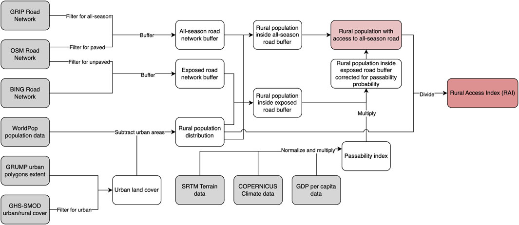
Figure 1. Overview of data processing.

2.1 Land cover data (urban/rural distinction)

Since the indicator measures the access of rural populations, it's important to define what is and what isn’t rural. This implementation uses primarily the DegUrba Methodology, proposed by the UN Expert Group on Statistical Methodology for Delineating Cities and Rural Areas (United Nations Expert Group, 2019). This approach has been deployed by the European Commission into the Global Human Settlement Layer (GHS-SMOD, 2023) dataset, which is designed to confer consistency for definitions based on population density and built-up area (European Commission et al., 2021). While GHS-SMOD offers the best available temporal resolution, being updated at least every 5 years, its spatial definition (1 km pixel) isn’t ideal, and in some cases urban areas can’t be well delineated. For this reason, data from NASA SEDAC CIESIN’s GRUMP (CIESIN et al., 2018), or Global Rural Urban Mapping Project, is also used. The Urban Extent Polygons provided by GRUMP are limited to the year of 1995, but have a better spatial definition due to generalization of pixels into concave hull vectors. Compatibilization of the two datasets was tackled by vectorizing the GHS-SMOD dataset and merging it to the GRUMP polygons. By doing so, urban areas consolidated before 1995 are better delineated, and their expansions’ up until 2020 is represented at a lower spatial resolution, reducing the total amount of “holes” in the urban extents. The overlap of urban areas from both datasets is used as the final urban land cover extent to be excluded from the analysis for RAI.

2.2 Population distribution

The source for population distribution data is WorldPop (World Pop, 2023). It uses national census data, projections and other ancillary data from countries to produce aggregated, 100 m² population data, making it the most spatially disaggregated population data currently available at global scale.

2.3 Road extent

One of the main issues identified in previous attempts to calculate RAI at global scale is ensuring that all roads are being taken into account. To respond to that, a redundancy strategy is used by simultaneously adopting three widely-recognized road datasets: the real-time updated, crowd-sourced OpenStreetMap (OSM, 2023), GLOBIO’s 2018 GRIP database (Meijer et al., 2018), which draws data mainly from official national sources, and Microsoft BING’s Road Detection Project (Microsoft Bing, 2023), which identifies roads through Neural Network models applied to optical satellite imagery. Each of these sources represents at least one advantage compared to the others:

• The GRIP database is the only global road network database containing information about the all-season status of roads, but to the detriment of its temporal resolution—which is restricted to the year of 2018—and its coverage, restricted to what national authorities could provide at the time.

• OpenStreetMap (2022 reference year) provides excellent temporal resolution and at least two attributes from which the all-season status can be derived: surface and hierarchy. Nevertheless, the network is limited by contributors’ interest in certain regions, which might skew the coverage towards urban centres to the detriment of rural areas.

• Microsoft Bing’s recent Road Detection (2022 reference year) project is used to ensure completeness. This dataset is completely derived from machine learning methods applied over optical high-resolution satellite imagery, and detected 1,165 km of roads missing from OSM, though there are currently no attributes associated to any of the roads.

The three datasets are filtered and put together in order to generate two final road subsets: all-season (paved) and exposed (unpaved). The distinction is important, as unpaved roads deteriorate rapidly and in a different way to paved roads (Workman and McPherson, 2019): unpaved roads are more exposed to water ingress to the surface, softening materials and making them vulnerable to traffic. This process is performed with command-line tools specific for each data source: osmfilter and osmconvert form the OSM data, and python’s geopandas for the remainder.

The first subset contains roads classified as all-season by GRIP and roads tagged as paved and/or as a hierarchy often (≥60%) associated with paved surfaces by OpenStreetMap (Supplementary Table S1). The population living within 2 km of these roads is considered to have full access to an all-season road. The second subset contains all roads identified by Microsoft Bing’s Road Detection project (as those aren’t qualified in any way) and roads tagged as unpaved and/or as any of the remaining hierarchy tags, given that they’re not also tagged as paved by OpenStreetMap.

The roads in the second subset are considered to be exposed to factors associated with difficulty of access. Their probability of being all-season is calculated by the superimposition of passability criteria, which are described in the following section. The population living within 2 km of these roads will be considered in equal proportion to the probability that the road provides all-season access (i.e., if it’s established that there’s a 10% chance that a road is all-season, only 10% of the population living within 2 km of it will be considered to have access to it).

2.4 Roads’ all-season status

The 2019 supplemental guidelines (Workman and McPherson, 2019) proposed that passability should equate to the all-season status of a road, along with the assumption that typically the wet season is when roads become impassable, especially so in steep roads.

This dataset implements a passability index, where each component is used as a multiplying factor ranging from near 0 to 1 over the population distribution layer whenever they’re located exclusively inside a buffer generated by an exposed (unpaved) road. The proposed use of passability factors relies on the following aspects:

• Climate. Precipitation has a significant effect on the condition of unpaved roads, being a significant factor in its deterioration. We use the Copernicus Programme’s (C3S, 2017) yearly accumulated precipitation data, which is made available freely at −30 km pixel resolution for reference year 2022.

• Terrain. The gradient and altitude of roads also has an effect on their passability. Steep roads become impassable more easily due to the potential for scouring during heavy rainfall, and also due to slipperiness as a result of the road surface materials used. Here this is drawn from slope calculated from SRTM Digital Terrain data (Jarvis et al., 2008), provided at −30 m pixel resolution.

• Road maintenance. The ability of local authorities to repair damage caused by precipitation and scouring is proposed as a correcting factor to the previous ones. Ideally, this would be measured by the % of GDP invested in road construction and maintenance, but this isn't available for all countries. For this reason, GDP per capita for reference year 2022 is adopted as a proxy, as provided by the World Bank (World Bank, 2023).

It’s important to note that, differently from the suggestions of datasets made by TRL (Workman and McPherson, 2019), we preferred datasets with at least medium spatial resolution, in raster format, and with temporal resolution of at least 1-year. This ensures that the results won’t be the exactly the same when RAI is calculated every year.

In order for RAI to account for the probability that the roads populations are using are all-season or not, the disaggregated factors for accessibility are applied to the spatialized disaggregated population data at pixel level through raster algebra. The final passability index is measured on a scale of 0–1, with 1 being 100% probability that the roads are all-season. For example, a road in a flat area with low rainfall and high investment in infrastructure maintenance would have an accessibility factor of 1.0, as this road is designed to be accessible all year round and the environmental effects on its impassability are minimal. The lower and upper thresholds for the each one of the factors ranges are close but never reach 0 and 1, ensuring that when multiplied, the final passability gets incrementally closer to 0 in the lower end and 1 in the higher end (Supplementary Table S2).

The multiplication of the climate and terrain factors (each ranging from 0.25 to 0.95) generates the first iteration of the passability criteria, which ranges from 6% to 90% (0.0625–0.9025). This first iteration does not take road maintenance into account (Supplementary Table S3).

The GDP per capita data is then normalized in such a way that a road maxed out in terms of precipitation and slope (accessibility score of 0.0625) in a country at the top of the GDP per capita range is brought to the higher end of the accessibility score 1), while the accessibility score of a road meeting the same passability conditions in a country where GDP per capita is towards the lower end is further lowered. A mathematical threshold is applied in order to ensure that values higher than 1 are replaced by the final range’s maximum (1, or 100%).

The multiplication of the three factors take place in a GIS environment, through raster algebra, with the smaller pixel size being the final resolution. The final index ranges from virtually 0 to 1 (Supplementary Table S4).

3 Data processing and results

Data processing takes place in Google Earth Engine, and begins with filtering out all the pixels overlapping areas classified as urban from the population layer. The result is a rural population raster layer at 100 m pixel resolution, shown in Figure 2.

Figure 2

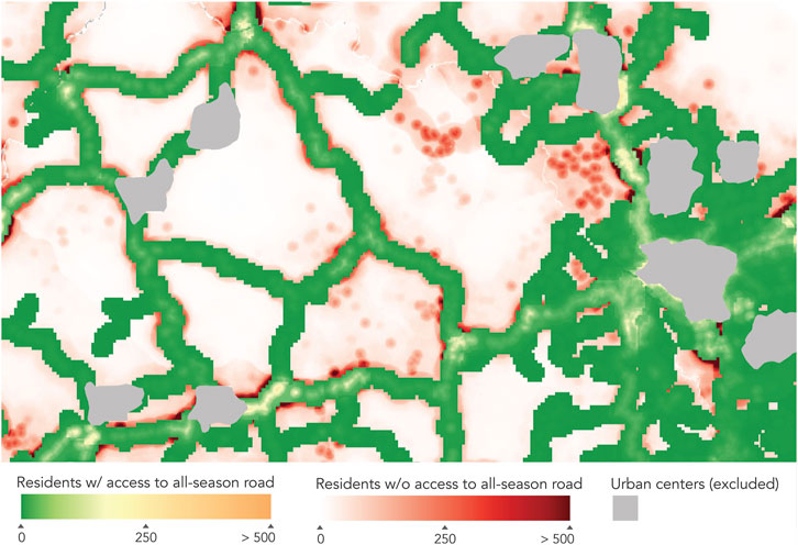
Figure 2. Showcase of the scale in which results are calculated in rural Democratic Republic of the Congo.

The two subsets of roads (all-season and exposed) have a 2 km buffer applied to them. As this operation is quite resource-intensive at a global scale, the roads are rasterized into 800 m wide pixels, a Euclidean distance calculation is performed, and all pixels with values higher than 2 km are filtered out.

The layers for precipitation, slope and road maintenance are rescaled and realigned to match the pixel grid in the rural population layer, allowing for raster algebra operations that do not require resampling. The three layers are multiplied by one another (limiting the upper threshold to 1), resulting in the passability index layer.

Pixels from the rural population layer falling over exposed road buffers have their values multiplied by the passability index. The resulting probability corrected population layer is combined with the population falling over all-season road buffers through raster algebra by making use of a maximum value rule. This ensures that whenever the same population pixel is intersected by buffers of the two road subsets, the largest value (the one not corrected by the passability index) is kept. The resulting layer represents the rural population with access to an all-season road.

The total rural population and the rural population with access to an all-season road raster layers are each used as input for zonal statistics operations to determine the total sum by country. The population with access is divided by the total rural population in order to obtain the proportion, which is the final Rural Access Index (RAI).

3.1 Data validation

Several checks were performed in order to assess the validity of the data produced. Construct validity is assessed by calculating the correlation coefficient with other previous attempts at calculating RAI. The two other pre-existing datasets covering RAI at national scale globally are distributed by NASA SEDAC’s CIESIN (CIESIN, 2022) and by Azavea (Azavea, 2019). Both implemented simpler methodologies, either by using exclusively the GRIP database or removing roads not classified as all-season or by removing roads not tagged as very high hierarchy level from OpenStreetMap. Supplementary Table S5 presents the Pearson coefficient found for each of the datasets. Though the coefficients are high (>80), it’s adequate that they aren’t extremely high (>95), showing that implementing the present method does yield different results due to the better road extent coverage and modeling of all-season status.

Convergent validity is assessed through correlation coefficients regarding variables that are expected to correlate with rural accessibility. Here GDP per capita and the Human Development Index (HDI) for the same reference year (2022) are used. Supplementary Table S6 presents the Pearson coefficients found for each variable. It’s telling that RAI has a high correlation (0.76) with HDI, as both can be used as evidence to shield or validate claims about the state of social justice or injustice.

3.2 Known limitations

3.2.1 Scale considerations

Some very small countries, such as Small Island Developing States (SIDS), are excluded from the final result, as those are considered to be entirely urban by the land cover layers used (GRUMP and GHS-SMOD). The remaining small island states with rural populations will tend to achieve very high scores, as the road infrastructure distribution will tend to be much more homogeneous where the rural-urban divide is less clear.

3.2.2 Mobility infrastructure not included

While access to all-season roads offers a fair representation of rural population’s overall accessibility and mobility, it might provide and under-assessment in places where transportation by other means, such as motorcycle trails and navigable waterways, are relevant. Communities living in the Amazon rainforest, for example, are highly dependent on fluvial transportation, which represented as much as 13% of the total modal share in Brazil as a whole in 2012 according to the Brazilian Agency for National Aquatic Transportation (ANTAQ, 2013). To respond to this limitation, we reiterate the 2019 TRL methodology (Workman and McPherson, 2019) recommendation for the creation of a secondary, supplementary indicator to allow countries to take into account local infrastructure that might not be included in the standard RAI measurement. Besides, selected road data sources (OSM, GRIP and Bing) are subject to data quality and coverage variations, that can affect results, particularly in developing countries where OSM data coverage is less uniform, potentially amplifying innacuracies.

3.2.3 Ground-truthing and construct validity

No ground-truth is assessed at any point in this implementation. We envision a new project specifically to this end, with the final objective of refining passability factors and the overall methodology. The project would assess road conditions through remote or on-site methods such as visiting and interviewing communities to ascertain how long roads might be closed due to climate or terrain issues. The results of the ground truthing would then be compared to the desktop assessment, and used to refine the accessibility factors as necessary, enhancing the indicator’s robustness.

3.2.4 GDP as a proxy for road maintenance

While data on infrastructure maintenance related to preserving the existing transport network exists, it’s collected by ITF only for OECD countries. In either case, both datasets do not provide for spatial variation, and are available at national scale only. While the possibility of using a dataset of machine learning predicted gridded values was assessed, we considered it to bring unnecessary bias. For these reasons, this variable should be revised in the future, should a better option become available.

3.3 Conclusion

The challenge of establishing an accurate and replicable method for measuring SDG 9.1.1 has been successfully tackled by the World Bank, custodian of the indicator, with the publication of its last methodology in 2016 and the endorsement of TRL supplementary guidelines in 2019. By producing the first ever implementation of the 2019 Supplementary Guidelines at global scale, we aimed at consolidating it as the most up-to-date methodology while also unifying propositions made by other interested parties. The method is highly sustainable, as required data collection is kept simple and independent of local efforts, making use of global-coverage spatial datasets to assess the all-season status of roads without putting extra burden on countries to collect additional data. This implementation should help ensure the continued use of RAI as the key rural accessibility indicator globally and within the SDG indicators framework, by maximizing the use of geospatial data with global coverage and minimizing the burden of additional local data collection.

Data availability statement

Data is available at the SDG Transformation Center Data Hub (https://sdgtransformationcenter.org/geospatial), and code for generating results at SDSN’s Github page (https://github.com/sdsna/rai).

Author contributions

GI: Conceptualization, Data curation, Formal Analysis, Investigation, Methodology, Software, Validation, Visualization, Writing–original draft, Writing–review and editing. ED: Conceptualization, Formal Analysis, Funding acquisition, Project administration, Resources, Supervision, Validation, Writing–review and editing. GF: Formal Analysis, Project administration, Validation, Writing–review and editing. GL: Formal Analysis, Funding acquisition, Project administration, Resources, Supervision, Validation, Writing–review and editing.

Funding

The author(s) declare that no financial support was received for the research, authorship, and/or publication of this article.

Conflict of interest

The authors declare that the research was conducted in the absence of any commercial or financial relationships that could be construed as a potential conflict of interest.

Publisher’s note

All claims expressed in this article are solely those of the authors and do not necessarily represent those of their affiliated organizations, or those of the publisher, the editors and the reviewers. Any product that may be evaluated in this article, or claim that may be made by its manufacturer, is not guaranteed or endorsed by the publisher.

Supplementary material

The Supplementary Material for this article can be found online at: https://www.frontiersin.org/articles/10.3389/frsen.2024.1375476/full#supplementary-material

References

ANTAQ – Agência Nacional de Transportes Aquaviários, (2013). Anuário estatístico aquaviário. Brasília: ANTAQ.

Google Scholar

Azavea, (2019). Rural access index measurement tool. Retrieved May 9, 2023, from https://rai.azavea.com/.

Google Scholar

Center for International Earth Science Information Network (Ciesin), (2022). Rural access index. Palisades: NASA socioeconomic data and applications center (SEDAC). Accessed https://services2.arcgis.com/IsDCghZ73NgoYoz5/arcgis/rest/services/CIESIN_SDG_911_v1/FeatureServer.

Google Scholar

Center for International Earth Science Information Network Columbia University, (2018). “CUNY institute for demographic research, international food policy research institute, the World Bank, and centro internacional de Agricultura tropical,” in Global rural-urban mapping project, version 1 GRUMPv1: urban extent Polygons Palisades: NASA Socioeconomic Data and Applications Center SEDAC. Center for International Earth Science Information Network Columbia University Columbia, NY, USA.

Google Scholar

Copernicus Climate Change Service, (C3S) (2017). ERA5: fifth generation of ECMWF atmospheric reanalyses of the global climate Co-Pernicus climate change service climate data store (CDS). Available online: accessed on 10/02/2023 https://cds.climate.copernicus.eu/cdsapp#!/home.

Google Scholar

European Commission, (2021). Applying the Degree of Urbanisation— a methodological manual to define cities, towns and rural areas for international comparisons. Statistical office of the European union 2021 edition. Luxembourg: Publications Office of the European Union. doi:10.2785/706535

CrossRef Full Text | Google Scholar

GHS-SMOD (2023). R2023A - GHS settlement layers, application of the Degree of Urbanisation methodology (stage I) to GHS-POP R2023A and GHS-BUILT-S R2023A, multitemporal (1975-2030). Luxembourg European Commission, Joint Research Centre (JRC). PID: doi:10.2905/A0DF7A6F-49DE-46EA-9BDE-563437A6E2BA

CrossRef Full Text | Google Scholar

Jarvis, A., Reuter, H. I., Nelson, A., and Guevara, E. (2008). Hole-filled SRTM for the globe version 4. available from the CGIAR-CSI SRTM 90m Database https://srtm.csi.cgiar.org/.

Google Scholar

Meijer, J. R., Huijbregts, M. A. J., Schotten, C. G. J., and Schipper, A. M. (2018). Global patterns of current and future road infrastructure. Environ. Res. Lett. 13 (6), 064006. doi:10.1088/1748-9326/aabd42

CrossRef Full Text | Google Scholar

Microsoft Bing (2023). Road detections from Microsoft Maps aerial imagery [Data set] GitHub Repos. https://github.com/microsoft/RoadDetections.

Google Scholar

OpenStreetMap contributors, (2023). OpenStreetMap database. Cambridge, UK: OpenStreetMap Foundation. © OpenStreetMap contributors. Available under the Open Database Licence from: openstreetmap.org.

Google Scholar

Roberts, P., Shyam, K. C., and Rastogi, C. (2006). “Rural access index: a key development indicator,” in Transport paper TP-10 (Washington, DC, USA: World Bank).

Google Scholar

Schiavina, M., Melchiorri, M., and Pesaresi, M. (2023). GHS-SMOD R2023A - GHS settlement layers, application of the Degree of Urbanisation methodology (stage I) to GHS-POP R2023A and GHS-BUILT-S R2023A, multitemporal (1975-2030). Luxembourg European Commission, Joint Research Centre (JRC). PID: http://data.europa.

Google Scholar

Workman, R., and McPherson, K. , and TRL (2019). “Measuring rural access using new technologies: supplemental guidelines,” in ReCAP GEN2033D (London, UK: ReCAP for DFID).

Google Scholar

Workman, R., and McPherson, K. (2021). Measuring rural access for SDG 9.1.1. Trans. GIS 25 (2), 721–734. doi:10.1111/tgis.12721

CrossRef Full Text | Google Scholar

World Bank (2023). GDP per capita, PPP (CONSTANT 2017 INTERNATIONAL $). Available online: accessed on 10/02/2023 https://datacatalog.worldbank.org/search/dataset/0037712/World-Development-Indicators .

Google Scholar

World Bank (2023). SDG 9.1.1.- rural access index (RAI) official data data set. https://datacatalog.worldbank.org/search/dataset/0038250.

Google Scholar

World Bank (2016). Measuring rural access using new technologies. World Bank Washington, DC, USA.

Google Scholar

World Pop (2023). Global Project population data: estimated residential population per 100x100m grid square. [Data set]. Availa-ble online: Accessed on 10/02/2023 https://worldpop.org .

Google Scholar