A workflow for extracting ungulate trails in wetlands using 3D point clouds obtained from airborne laser scanning

Ungulates and other mammalian herbivores can create trails in dense vegetation by trampling and browsing. This can affect vegetation structure and result in the fragmentation of closed, high vegetation, with subsequent impacts on biodiversity. Manually mapping trails in the field or from aerial photographs can be challenging and time-consuming, especially in inaccessible or difficult-to-access habitats such as wetlands and if trails occur beneath the canopy of woody plants (i.e., trees and shrubs) or in other tall vegetation (e.g., reed). Airborne laser scanning (ALS) provides an alternative method because Light Detection and Ranging (LiDAR) can record returns from both the canopy and the ground, as some laser pulses pass through gaps in the vegetation, resulting in highly accurate and dense three-dimensional (3D) point clouds. Here, we present a workflow for extracting ungulate trails using 3D point clouds obtained from country-wide ALS surveys, illustrated by red deer trampling in reedbeds within a 36 km² marsh area of a Dutch nature reserve. The workflow starts by pre-processing to retile the LiDAR point clouds to designated tiles and removes outliers from the raw data. The (near-)terrain points are then segmented using an iterative filtering algorithm, and digital terrain models are generated with a user-defined resolution. Finally, trail cells are extracted by thresholding the residuals from iterative Laplacian smoothing and then refined by sparse 3D structure tensor voting. The parameters of the workflow were optimized with comprehensive sensitivity analyses. Applying the workflow resulted in a classification of trail and non-trail grid cells at 10 cm resolution across the study area. Compared to manually labeled ground truths, the results showed an overall accuracy of 93% and 90% in regions of red deer grazing only and both geese and red deer grazing, respectively. To test its transferability, the workflow could be applied to other LiDAR data (e.g., ALS surveys from another flight campaign in the same study area or in a different country), to other nature areas (e.g., other rewilding sites or other wetlands), and to other ungulate species (e.g., domesticated livestock or other native large herbivores).

1 Introduction

In many nature reserves in Europe, ungulates such as horses, cattle or red deer are introduced as ecosystem engineers to influence vegetation structure through trampling, browsing and grazing and to create diverse habitats for plants and animals (Bakker et al., 2018; Cornelissen, 2017; Müller et al., 2017). In addition to habitat heterogeneity, they can also create trails, leading to habitat fragmentation, which is one of the causes of declines in biodiversity (Lindenmayer and Fisher, 2013). Trails are typically linear features and evaluating their impact on ecosystems and biodiversity requires quantitatively delineating trails over large areas. Methods for linear object extraction from 2D images exist (Cao and Zhang, 2020; Chowdhary and Acharjya, 2020; Humeau-Heurtier, 2019; Liu and Peng, 2009), but extracting trails in three-dimensional (3D) vegetation can be challenging because trails are often covered by tall vegetation (e.g., overhanging reed, shrubs and trees) which makes them difficult to detect from aerial images.

Light detection and ranging (LiDAR) technology employs pulsed laser beams to measure the time of flight from a reflected object to return to the receiver. This offers an efficient way to obtain highly accurate geometric information of objects in the form of 3D point clouds (Vosselman and Maas, 2010). Airborne LiDAR systems emit laser beams from an airborne platform and thereby receive return signals from vegetation (leaves, branches, stems) or the ground. Since laser pulses can produce multiple returns, which reflect from canopy and sub-canopy elements, understory, and the ground when unobstructed, they are widely used in forestry, ecology and biodiversity research to map the 3D structure of vegetation (Bässler et al., 2011; Guo et al., 2017; Gonzalez et al., 2018; Bakx et al., 2019). Compared to remote sensing imagery (e.g., RGB or multispectral aerial photographs), LiDAR point cloud data offers distinct advantages for detecting trail features in vegetated environments. First, LiDAR captures elevation data at high spatial resolution and with sub-meter vertical accuracy, allowing for the detection of subtle depressions in terrain such as ungulate trails. Second, because laser pulses can obtain terrain information through gaps in the vegetation canopy and with returns from multiple vertical layers (e.g., ground, understory, and canopy), LiDAR is particularly well-suited for mapping features beneath dense or understory vegetation (Štular et al., 2012; Thompson, 2020). However, optical imagery often fails due to occlusion or lack of contrast. These properties make LiDAR highly suitable for identifying trails in marsh habitats.

Several methods have been developed for extracting linear features from airborne LiDAR point clouds, including road centre line and edge extraction (Alshawabkeh, 2020; Hui et al., 2016), linear object detection in urban scenarios (Daniels et al., 2007; Lari and Habib, 2014), archaeological feature extraction (Seitsonen and Ikäheimo, 2021; Thuestad et al., 2021), and identification of hedgerows and tree lines (Lucas et al., 2019). In wetlands, LiDAR has been used to classify land cover types and habitats (Koma et al., 2021a) and to quantify the 3D structure of reedbeds (Koma et al., 2021b). However, to our best knowledge, there is no study that has yet analysed the trampling and browsing effects of ungulates on reedbeds using LiDAR point clouds. Understanding the impact of ungulates is of crucial importance for biodiversity conservation and habitat management.

Here, we present a workflow for extracting ungulate trails in wetlands from raw 3D point clouds of country-wide airborne laser scanning (ALS) surveys. We focus on red deer trails in reedbeds of an extensive marsh area in the Netherlands where this ungulate was introduced in 1992 and subsequently reached high densities (Cornelissen et al., 2014). Our work consists of pre-processing the LiDAR point clouds, filtering of (near-)terrain points, reconstructing Digital Terrain Models (DTMs) and subsequent classification of trail and non-trail grid cells at 10 cm resolution using Laplacian-smoothed DTMs and sparse 3D structure tensor voting. In this work, “trails” refer to grid cells of the DTMs that exhibit topographic depression signatures characteristic of ungulate trampling. The specific objective is to delineate trail grid cells, enabling high-resolution mapping of trail distribution and reedbed fragmentation. We optimized the parameters of the workflow with a comprehensive sensitivity analysis and validated the workflow with manually labelled point clouds.

2 Study area and material

2.1 Study area

The study was conducted in the Oostvaardersplassen nature reserve, a eutrophic wetland in the polder Zuidelijk Flevoland located in the centre of the Netherlands (Figure 1). It is both a Ramsar site (No. 427) and a Natura 2000 site (site code: NL9802054) for breeding and wintering wetland birds. The wetland consists of a marsh (36 km²) and a “dry” border zone with grasslands (20 km²). To create a diverse landscape in the border zone, cattle and horses were introduced in 1983/1984. In 1992, red deer (Cervus elaphus) were introduced to help decrease the ongoing establishment of shrubs and trees at that time. The area is fenced and there are no large predators such as wolves or bears. As the number of ungulates was not controlled, their numbers grew exponentially and in 2010 maximum numbers were reached, leading to very high densities of >200 animals per km² in the border zone. In 2018, the management changed because the landscape was no longer diverse and instead dominated by shortly grazed grasslands, which resulted in a decrease of bird diversity. From 2018 onwards, the ungulate populations were controlled to much lower densities of <75 animals per km². Although all the ungulates can potentially enter the marsh from the border zone, only red deer make use of it. They enter the reedbeds from the grassland areas and look for shrubs and trees to forage on. Our workflow development focuses on the reed-dominated marsh of the study area (Figure 1) which has been subject to red deer trampling and grazing.

Figure 1

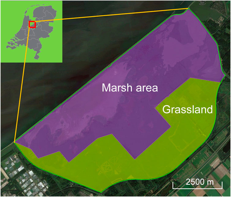
Figure 1. Overview of the study area Oostvaardersplassen in the Netherlands with its marsh area and grassland. The green polygon denotes the boundary of the study area (56 km²), the purple shaded area is the marsh (largely reedbed habitat and water, 36 km²), and the green shaded area is the border zone with grasslands (20 km²). The inset shows the location of the study area in the Netherlands.

2.2 Point clouds

We utilized the 3D point clouds collected during the fourth Dutch national ALS flight campaign, known as Actueel Hoogtebestand Nederland (AHN4), conducted between 2020 and 2022 (https://www.ahn.nl). The raw AHN4 point clouds, released in LAZ format (https://rapidlasso.com/laszip/), include x, y, z coordinates, intensity, the number of returns, and the GPS time of data acquisition. The AHN4 point clouds for the study area were captured in April 2020 and have an average point density of approximately 25 points per square meter. The original point clouds were downloaded from the AHN official public portal (https://hub.arcgis.com/maps/esrinl-content::ahn4-download-kaartbladen-1/explore). This included a total of seven original tiles (20DZ1, 20DZ2, 26AN2, 26BN1, 26BN2, 26AZ2, and 26BZ1). Each of these tiles has a spatial coverage of $5\text{\hspace{0.17em}km}\times 6.25\text{\hspace{0.17em}km}$. The total number of points of these tiles is 6,243,044,410 with a total volume of 42.3 GB. These original point clouds were used as the input into the presented workflow.

3 Methods

The workflow to delineate red deer trails within reedbeds consists of four steps (Figure 2): (1) Pre-processing; (2) Near-terrain filtering; (3) DTM reconstruction; and (4) Trail extraction.

Figure 2

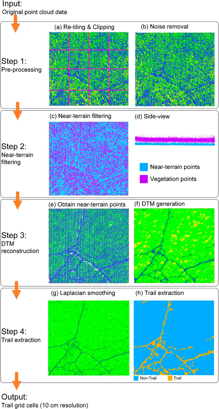
Figure 2. Workflow for extracting red deer trails in reedbed habitat. The point clouds are colorized by height from red (highest) and yellow (higher) to green (intermediate) and blue (lowest), unless otherwise indicated by a color legend.

3.1 Pre-processing

The downloaded AHN4 point clouds (i.e., seven tiles) of the study area were used as input for workflow step 1 (pre-processing). The pre-processing of the point clouds consists of three steps: (i) re-tiling; (ii) clipping, and (iii) outlier removal. The point cloud for input is large in storage space (i.e., the seven original tiles amount to ∼42.3 GB tile volume in LAZ format), which makes manipulating the data difficult. We therefore implemented a spatial extent-based re-tiling approach, which segments the original input point clouds ($5\text{\hspace{0.17em}km}\times 6.25\text{\hspace{0.17em}km\hspace{0.17em}tiles}$) into $50\mathrm{m}\times 50\mathrm{m}$ tiles. The generated tiles were then clipped using the polygon shapefiles of the marsh area. For the clipping, we implemented the winding number algorithm which parses points within polygons (Kumar and Mallikarjun, 2018).

Statistical outlier removal (SOR) was implemented to remove noise, e.g., points from water surface reflection and sparse higher vegetation points (Vosselman and Maas, 2010), using the method proposed in Rusu et al. (2008). Suppose $P$ is a set of 3D points, and for each query point $p_{query}\in P$, $\overline{d}$ is the mean distance of a query point to its $k$ nearest neighbors. For all points in $P$, the mean distance and standard deviation of the distances of their $k$ nearest neighbors are then determined. Only those points are kept which have distances that are close to the mean distance of the closest neighbours, using Equation (1).

$\left.P^k=\left.\left\{p_q\in P\right.\right|\left({\mu }_k-\alpha {\sigma }_k\right)\le \overline{d}\le \left({\mu }_k+\alpha {\sigma }_k\right)\right\}(1)$

Here, $\alpha$ is a density threshold coefficient, and ${\mu }_k$ and ${\sigma }_k$ are the mean and standard deviation of the distance from a query point to its $k$ closest neighbors. $P^k$ is the point set that is kept, i.e., after removing the outliers.

In summary, the raw ALS point clouds are first re-tiled into smaller spatial units to manage the large file sizes. Then, the tiles are clipped to the marsh boundary using polygon shapefiles. Finally, outliers are removed using the SOR method, which filters points based on their local neighbourhood distance distribution.

3.2 (Near-)terrain filtering

In workflow step 2 (near-terrain filtering), the reedbed points are removed and only the terrain and near-terrain points (i.e., ground and low vegetation points) within the study area are kept. A virtual 3D grid layer is used in this filtering approach which applies a horizontal boundary of the 3D point cloud with a user defined grid size $Siz{e}_g$ (Figure 3).

Figure 3

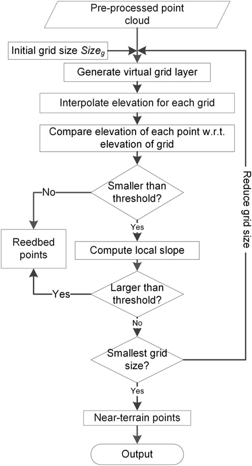
Figure 3. Filtering approach to obtain terrain and near-terrain points from an airborne laser scanning point cloud.

To construct a 3D grid layer from a given 3D point cloud, the first step is to determine the 3D bounding box that encloses the entire point cloud. This bounding box is then discretized into a structured array of 3D grid cells by dividing it along the $x,y,z$ axes. The number of divisions (bins) in each direction is determined based on a user-defined grid size. The origin of this grid, which is referred to as the “lower left point” of the bounding box, is denoted as $P_{\mathit{min}}$, which represents the minimum coordinate values in each axis direction. Each point in the point cloud is assigned a 3D grid index by comparing its coordinate $P^i$, where $i\in \left\{x,y,z\right\}$ with the corresponding coordinate of $P_{\mathit{min}}^i$ using Equation 2.

$n^i=\frac{P^i-P_{\mathit{min}}^i}{Siz{e}_g^i}\left(i\in x,y,z\right)(2)$

Here, $n^i$ denotes the grid index of a point along axis $i$, and $Siz{e}_g^i$ is the user-defined grid size in the respective direction.

Grids that contain no points are marked as empty and excluded from further processing. Figure 4 illustrates this process of subdividing the bounding box into grid cells. Initially, the grid size is chosen to be relatively coarse to facilitate efficient organization of the raw point cloud. In later stages of the workflow, particularly during iterative filtering, the grid size is progressively reduced to extract finer terrain detail.

Figure 4

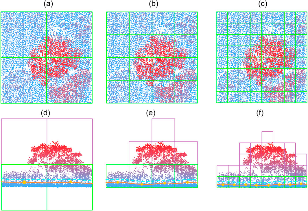
Figure 4. Iterative subdivision of the grids in the bottom layer to obtain a finer terrain surface. (a–c) are top view of three consecutive subdivisions, and (e–f) are the corresponding side views. The orange dots show the interpolated elevation of the grids based on the points inside each grid cell. The orange solid lines are the estimated terrain, and the cyan dashed lines indicate the threshold height.

After the creation of the 3D grids, only the bottom layer of the grids will be used for the height interpolation and iterative subdivision. The elevation of each grid in the bottom layer is interpolated by the points inside the grid using Equation (3).

$E_g=\frac{\sum E_p\left(\frac{L}{\sqrt{2}}-D_g\right)}{\sum \left(\frac{L}{\sqrt{2}}-D_g\right)}(3)$

Here, $E_g$ is the interpolated elevation of a grid at the geometric center, $E_p$ is the elevation of point $p$, $L$ is the size of the grid and $D_g$ is the distance from point $p$ to the geometric center of the grid.

The initial terrain surface is defined as the geometric centres of a set of coarse grid cells covering the area of interest. This coarse grid is constructed by dividing the bounding box of the point clouds at a coarse resolution level. The geometric centre of each cell is calculated as the midpoint of its horizontal extent $\left\{X,Y\right\}$, formatting a regularly spaced point set. In each iteration, the bottom layer is subdivided into finer cells, and the centres of these finer cells generate an updated virtual terrain surface for filtering (near-)terrain points (Figure 4).

For low vegetation like herbs and sedges, the terrain points and vegetation points might be difficult to separate, especially in places where trails are located. To prevent segmenting vegetation points as terrain points, a local terrain slope is introduced. Rather than using the geometric definition in Sithole and George (2004), the interpolated elevation of grids in each subdivision is used to compute a compensated local slope using Equation 4.

$S_p=\frac{H_p-H_g}{\sqrt{{\left(x_p-x_g\right)}^2+{\left(y_p-y_g\right)}^2}}(4)$

Here, $S_p$ is the local slope value, $H_p$ is the elevation value of point $p$, $H_g$ is the interpolated elevation value of the grid in which point $p$ is in, $x_p,y_p$ are the horizontal coordinates of point $p$, $x_g$ and $y_g$ are the geometric center of the grid. The procedure for filtering terrain and near-terrain points in an iterative approach is described in Algorithm 1.

Algorithm 1

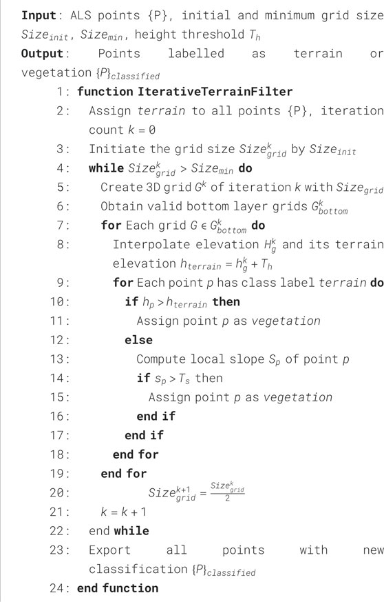
Algorithm 1. Iterative terrain points filtering from ALS point clouds.

In summary, a coarse 3D grid is created over the bounding box of the point clouds and elevation values at each grid cells are interpolated using local point distributions. Through iterative grid subdivision and terrain filtering, vegetation points are separated from terrain and near-terrain points based on height thresholds.

3.3 DTM reconstruction

In workflow step 3 (DTM reconstruction), the obtained terrain and near-terrain points are used to generate DTMs. We apply the Inverse Distance Weight (IDW) interpolation to estimate the elevation of each vertex of the DTM (Figure 5).

Figure 5

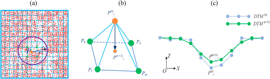
Figure 5. DTM generation using the obtained terrain and near-terrain points. (a) The elevation of point $\mathrm{P}$ on a vertex of the DTM is interpolated by the height of all terrain and near-terrain points (in red color) within radius $\mathrm{r}$. (b) A smoothing step is applied for each vertex based on adjacent neighboring vertices (green points). (c) Iterative Laplacian smoothing of the generated DTM profile in vertical direction. $\text{DT}{\mathrm{M}}^{\left(\mathrm{t}\right)}$ and $\text{DT}{\mathrm{M}}^{\left(\mathrm{t}+1\right)}$ are profiles of a trail at iteration t and t + 1, respectively.

As shown in Figure 5a, the points in red are the obtained terrain and near-terrain points using the method described above (Section 3.2). The blue grids are the DTM with a user-defined resolution. For a specific vertex $P$ of the DTM (orange point), its elevation is estimated by all red points within the neighborhood radius $r$ using Equation 5.

$H_p=\frac{\sum \frac{H_i}{d_i}}{\sum \frac{1}{d_i}}(5)$

Here, $H_p$ is the estimated elevation of vertex $P$ on the DTM, $H_i$ is the elevation of $i$-th point within radius $r$, and $d_i$ is its distance to vertex $P$. The generated DTM will then be used for workflow step 4 (trail extraction).

In summary, the filtered terrain and near-terrain points are used to construct DTMs using IDW interpolation. Elevations at DTM vertices are computed using nearby points within a defined radius.

3.4 Trail extraction

In workflow step 4 (trail extraction), the Laplacian smoothing method is first employed to smooth the DTM mesh (Häufel, Böge, and Bulatov, 2020; Nealen et al., 2006). As shown in Figure 5b, point $P^{\left(t\right)}$ is one vertex on the DTM (orange point), and points $P_k$, $P_l$, $P_m$ and $P_n$ are its neighbouring vertices (green points). The smoothing procedure is defined by Equation 6.

$P_i^{\left(t+1\right)}=P_i^t+{\lambda ∆P}_i^t(6)$

Here, $P_i^{\left(t+1\right)}$ is the smoothed point of vertex $P_i^{\left(t+1\right)}$ after $t$ iteration, $\lambda$ is a coefficient and $\Delta P_i^{\left(t\right)}$ is defined by Equation 7.

${∆P}_i^{\left(t\right)}=\frac{1}{N_i}{\displaystyle \sum _{j\in N_i}}{P}_j-P_i(7)$

Here, $N_i$ is the number of neighboring points used for smoothing P_i is the query point and P_j is one of the neighbouring points. As illustrated in Figure 5c, the Laplacian smoothing is applied iteratively on the smoothed DTM mesh. $DT{M}^{\left(t\right)}$ is a profile of the DTM in the previous iteration and $DT{M}^{\left(t+1\right)}$ is the DTM of the next iteration. Note that only the elevation values $z$ are used for smoothing (Figure 5c). Thus, the horizontal distances between the DTM vertices remain unchanged.

For classifying trail grid cells, the smoothed DTM is then used as input. As illustrated in Figure 5c, ${DTM}^{\left(t\right)}$ is a profile of a trail at iteration $t$ and $DT{M}^{\left(t+1\right)}$ is the smoothed profile at the consecutive iteration using Laplacian smoothing. The vertices in the shallow area of the trail were smoothed such that their elevation (z) is higher compared to that of the previous iterations. For example, the elevation of point $P_i^{\left(t+1\right)}$ is higher than that of point $P_i^{\left(t\right)}$. Thus, subtracting the elevation of the two DTMs results in a map of elevation difference where areas of trails show the largest elevation changes. Equation 8 defines the elevation changes of DTMs from two consecutive Laplacian smoothing iterations.

$\Delta H=D{TM}^{\left(t\right)}-D{TM}^{\left(t+1\right)}(8)$

Here, $\Delta H$ is the calculated height difference. The grid cells of trail areas can then be determined by Equation 9.

$\left.P_{trails}=\left.\left\{p_k\in P\right.\right|\Delta H\le \left({\mu }_{\Delta H}-\kappa {\sigma }_{\Delta H}\right)\right\}(9)$

Here, $P_{trails}$ are the points in the trail area, $p_k$ are the trail points, $P$ is the entire point sets, ${\mu }_{\Delta H}$ and ${\sigma }_{\Delta H}$ are the mean and standard deviation of $\Delta H$, and $\kappa$ is the coefficient. The trail extraction step thus results in each grid cell being classified as “Trail” or “Non-Trail” (Figure 2h).

The obtained “Trail” points are then cleaned using the SOR method described in Section 3.1. After that, a spatial clustering algorithm is applied to identify patches (i.e., clusters) of connected points based on the results from the Laplacian smoothing of the DTM (Cohen and Deschamps, 2001). This algorithm performs spatial clustering of a given set of 3D points $P=\left\{P_1,P_2,\dots ,P_N\right\}$ based on a connectivity criterion defined by a radius $r$. The goal is to partition $P$ into clusters $C_1,C_2,\dots ,C_k$ such that for any two points $p_i$ and $p_j$, they belong to the same cluster if there exists a path of points $p_i,p_{n_1},p_{n_2},\dots ,p_j$ where each consecutive pair of points $p_a$ and $p_b$ satisfies: $d\left(p_a,p_b\right)\le r$, here $d\left(*\right)$ is the Euclidean distance computation function. The algorithm begins by constructing a KD-tree for efficient nearest neighbor searching. For each point $p_i$, a radius search retrieves the set of neighors $N_i$, such that $\left.N_i=\left.\left\{p_j\in P\right.\right|{‖p_i-p_j‖}_2^2\le r^2\right\}$. Then a union-find data structure also known as Disjoint Set Union (DSU) is used to efficiently merge points into connected components, where each point $p_i$ initially represents its own cluster. When $p_i$ finds a neighbor $p_j$ with $j>i$, then a union operation is performed using Equation 10.

$union\left(i,j\right)\to find\left(i\right)=find\left(j\right)(10)$

After processing all points, clusters are identified by extracting the connected components where all points sharing the same root representative in the DSU form a cluster. This results in a partition of $P$ into $k$ clusters $C_1,C_2,\dots ,C_k$ using Equation 11.

$C_i=\left.\left\{p_j\right.\right|find\left(j\right)=r_i\},\forall \mathrm{j}\in \mathrm{P}(11)$

The clusters are then used to extract linear features and to refine the trail extraction results. To achieve this, a 3D structure tensor $S\in R^{3\times 3}$ is calculated at the neighborhood and 3D sparse tensor voting is applied (Jörgens and Moreno, 2015) to enhance the linear feature extraction and to remove small, non-linear and isolated clusters. The dimension of a neighborhood is determined as follows: Suppose $p_i={\left(x_i,y_i,z_i\right)}^T$ are the coordinates of a point $p_i$, and $T$ denotes the transpose of the matrix. Then the centroid of all the neighborhood points is determined by Equation 12.

$\overline{p}=\frac{1}{n}{\displaystyle \sum _{i=1}^n}{p}_i(12)$

Here, $n$ is the number of points in the neighbourhood. The 3D structure tensor $M$ of those points is then defined by Equation 13.

$M=\frac{1}{n}{Q}^{T}Q(13)$

Here, $Q={\left(p_1-\overline{p},p_2-\overline{p},\dots ,p_n-\overline{p}\right)}^T$. $M$ is a symmetric matrix and can be decomposed as $M=RI{R}^T$, $R$ is a rotation matrix and $I$ is a diagonal positive definite matrix in this case. The elements of $I$ are the eigenvalues of matrix $M$. The three eigenvalues are positive, can be denoted by ${\lambda }_1,{\lambda }_2,{\lambda }_3$, and are sorted such that ${\lambda }_1>{\lambda }_2>{\lambda }_3$. The corresponding eigenvectors are $v_1,v_2,v_3$, respectively. (Weinmann et al., 2015). Thus, Equation 13 can be rewritten to Equation 14 as follows:

$M={\displaystyle \sum _{i=1}^3}{\lambda }_i{v}_i{v}_i^T(14)$

The linearity, planarity and sphericity of the structure tensor are defined as follows (Equation 15):

$\begin{array}{l}L=\frac{{\lambda }_1-{\lambda }_2}{{\lambda }_1+{\lambda }_2+{\lambda }_3}{v}_1{v}_1^T\\ P=\frac{{\lambda }_2-{\lambda }_3}{{\lambda }_1+{\lambda }_2+{\lambda }_3}\left(v_1{v}_1^T+v_2{v}_2^T\right)\\ S=\frac{{\lambda }_3}{{\lambda }_1+{\lambda }_2+{\lambda }_3}\left(v_1{v}_1^T+v_2{v}_2^T+v_3{v}_3^T\right)\end{array}(15)$

The sparse 3D structure tensor defined in Equation 14 can then be reformulated as Equation 16:

$M=L+P+S(16)$

Based on the above decomposition, sparse 3D structure tensor voting is applied on the obtained point clusters (Medioni et al., 2000). In this workflow, the linear voting field is computed as given in Figure 6.

Figure 6

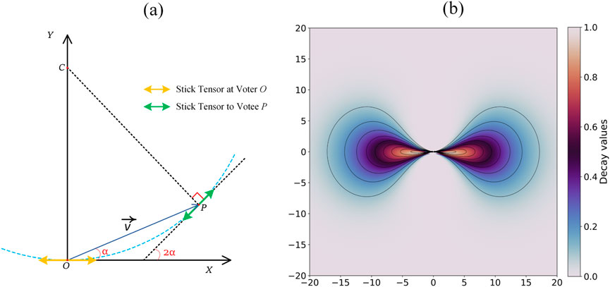
Figure 6. Linear tensor voting direction and the decay of the voting strength. (a) Voting from point $O$ to point $P$. (b) The voting weight of the voting field.

The direction of the voting tensor $O$ to position $P$ is obtained by rotating the voting tensor direction with angle $2\alpha$, as denoted by Figure 6a. Here, $\theta$ is the angle between vector $\overrightarrow{OX}$ and $\overrightarrow{OP}$. Equation 17 is used to define the weighting function which reduces the strength of the vote with the arc length $\breve{OP}$ and the curvature $k$.

$W_{sv}=\left\{\begin{array}{l}\frac{l^2}{2{\sigma }^2}-k^2\left(\alpha \le \frac{\pi }{4}\right)\\ 0\left(otherwise\right)\end{array}\right.(17)$

Here, $l=\frac{\left|\overrightarrow{v}\right|2\alpha }{\sin \left(2\alpha \right)}$, $k=\frac{2\sin \left(2\alpha \right)}{\left|\overrightarrow{v}\right|}$, and $\sigma$ is a scale parameter which is defined by the radius that is used for computing the local structure tensor within its neighborhood. The voting tensor propagates its saliency to the neighboring locations and aggregates the saliency that associated with the 3D structure tensor.

In summary, a Laplacian smoothing procedure is iteratively applied to the generated DTMs to capture subtle depressions that are indicative of “trails.” Then, trail locations are identified by computing elevation differences between two consecutively smoothed DTMs. Grid cells with high residuals are classified as “trail.” A spatial clustering algorithm is then applied to group connected trail cells, and sparse 3D structure tensor voting is applied to refine the output by enhancing linear features and removing noisy, non-linear clusters.

3.5 Accuracy assessment

To validate the accuracy of the workflow for extracting ungulate trails, we randomly placed a total of 100 plots of $30\mathrm{m}\times 30\mathrm{m}$ size in our study area. All 100 sample plots were not located in water areas nor at the water-reedbed boundary to avoid incomplete plots. Half of the plots were randomly placed in those reedbed areas of the marsh in which only red deer are grazing (red colour in Figure 7), and the other half where both red deer and graylag geese (Anser) are grazing (yellow colour in Figure 7). Areas in which only geese are grazing were not considered (green colour in Figure 7). Besides red deer, graylag geese are also grazing reedbeds, but they mainly feed on young reed shoots that occur near open water (Bakker et al., 2018). To test whether goose grazing has an influence on the trail extraction results in areas where both red deer and geese co-occur, we performed the method validation on areas of the reedbed that have either been subject only to red deer activity or to both red deer and graylag geese grazing. These areas are mapped yearly as part of the breeding bird monitoring in the marsh (Beemster et al., 2020).

Figure 7

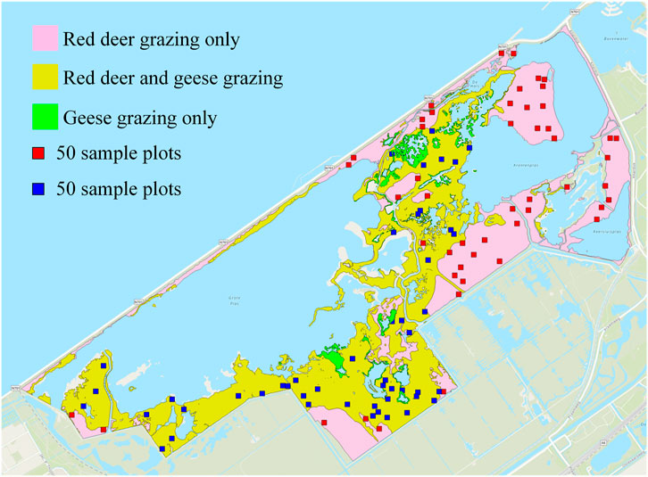
Figure 7. For method validation, a total of 100 sample plots were randomly placed within the reedbeds of the marsh area that were grazed by red deer (Cervus elaphus) only and grazed both by red deer and graylag geese (Anser anser). Areas with only geese grazing were not included.

The accuracy of trail extraction was evaluated by comparing the results from the presented workflow with the results from manually created ground truths. Manual labelling of the point clouds was done by using the segment tool of the CloudCompare software (https://cloudcompare.org/). The 3D point cloud data were first loaded and then segmented using the DB panel of CloudCompare. Then, the segmentation mode was activated (using the Scissors icon in the toolbar), and a closed polygon was drawn around the desired points by clicking sequentially. Once the selection was complete, the class labelling button was used to classify the selected “trail” points as class “1” and the rest of the points as “non-trail” points (classified as “0”). Areas of “non-trail” depict higher elevations compared to areas of “trail.” After manually labelling the discrete points, a DTM of 10 cm resolution was generated for each plot using the same method as described in Section 3.2 (DTM reconstruction). The class of each grid point was assigned to that of the closest point from the manually created ground truth. A total of 9,000,000 grid points were finally labelled as ground truth across the 100 sample plots. For each plot, the overall accuracy $Acc$ was used as the evaluation metric, which is defined in Equation 18.

$Acc=\frac{TP+TN}{TN+TN+FP+FN}(18)$

Here, $TP$ (true positives) are the correctly extracted trail cells of 10 cm size, $FP$ (false positives) represent non-trail cells that were wrongly extracted as trails, $FN$ (false negatives) are trails cells that are incorrectly segmented as non-trails, and $TN$ (true negatives) are the correctly segmented non-trail cells. The overall accuracy was calculated for each of the 100 sample plots.

3.6 Sensitivity analysis

The presented workflow uses seventeen parameters (Table 1). The specific settings of the parameters for the application in our study area are given in Table 1. The choice of these specific parameter values was informed by sensitivity analyses or constrained by the specific characteristics of the point cloud data from our study area.

Table 1

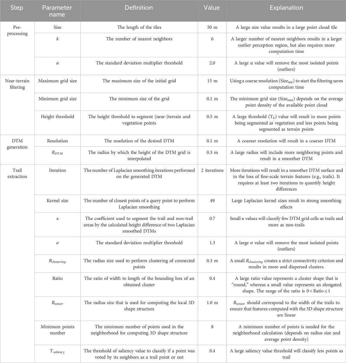
Table 1. Parameters of the workflow with the specific settings (“Value’) that were used in the study area.

A total of twelve parameters were tested with a sensitivity analysis (Table 2). For each of these twelve parameters, ten experiments with different parameter values were conducted (Table 2). All other parameters were kept constant (as given in Table 1). Five of the parameters ($Size$, $k$, $\alpha$, $Maximumgridsize$, and $Resolution$) were not subject to a sensitivity analysis for the following reasons. $Size$, $Maximumgridsize$, $k$, and $Resolution$ are the parameters which influence the computation time rather than the output accuracy of the presented workflow. Their values were chosen to make the workflow computationally efficient. The parameter $\alpha$ was kept constant because the used point clouds were all collected with the same flight campaign, i.e., the overall quality of the data in our study area is similar.

Table 2

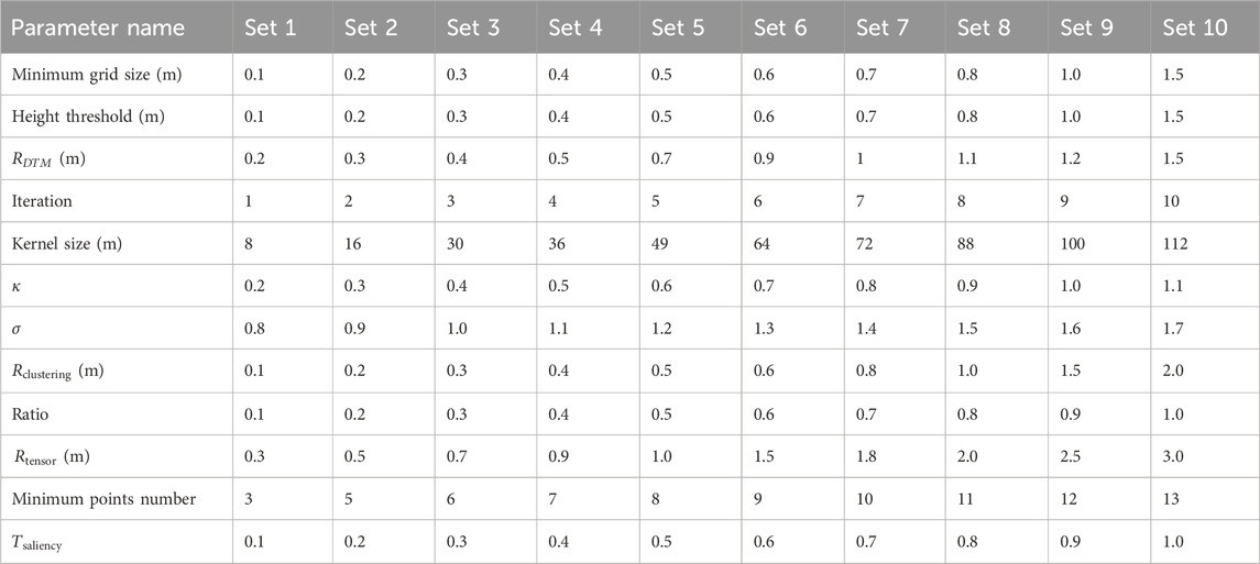
Table 2. The parameter settings for the sensitivity analysis. Ten experiments (set 1–10) were conducted for each parameter while keeping all other parameters as specified in Table 1.

For the near-terrain filtering (workflow step 2), the relevant parameters are $Maximumgridsize$, $Minimumgridsize$, and $Heightthreshold$ (Table 1). To evaluate the accuracy of this workflow step when changing the parameters (Table 2), we manually labelled all vegetation and near-terrain points in the 50 sample plots which were exclusively grazed by red deer (see example in Supplementary Figure A1). The manually labelled point clouds where then compared to the automatically segmented point clouds from the workflow using different parameters settings for the $Minimumgridsize$ (Supplementary Figure A2) and for the $Heightthreshold$ (Supplementary Figure A3).

For the DTM reconstruction and trail extraction (workflow steps 3 and 4), the accuracy was evaluated based on the manually created trail and non-trail ground truth of the 50 sample plots that are placed in the area that is exclusively grazed by red deer.

4 Results

4.1 Workflow results

4.1.1 Pre-processing

The pre-processing step first loaded the seven original tiles of the raw point cloud data which cover the studied marsh area (Figure 8a). These seven tiles of point cloud data were then retiled to square plots of $50m\times 50m$ size (Figure 8b) and clipped to the boundary polygon of the marsh area (Figure 8c). After clipping, a total of 490,234,336 points were kept. The final step of pre-processing then removed the outliers (see parameter settings in Table 1) which resulted in a total of 470,279,992 points that were kept for the near-terrain filtering step. The ∼20 million removed points mainly characterized sparse higher vegetation points and water surface reflections. Their removal allowed us to improve the efficiency of the workflow by focusing on terrain and near-terrain points.

Figure 8

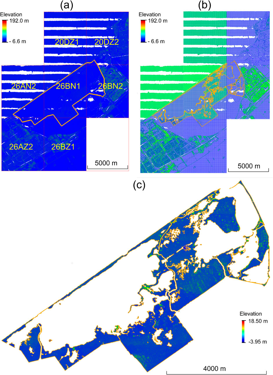
Figure 8. Pre-processing of the original raw point clouds. (a) Geo-location of the study area with the seven raw tiles from the AHN4 point clouds. (b) The raw tiles are retiled into $50m\times 50m$ square plots. (c) Clipping and outlier removal is performed on the retiled point clouds of the studied marsh area. The polygon in orange is the boundary of the studied marsh area. White areas indicate areas with water.

4.1.2 (Near-)terrain filtering

The cleaned point cloud was the input for obtaining the near-terrain points (Figure 9). The filtering started with a maximum grid size of 15 m and ended with a minimum grid size of 0.1 m, using a height threshold of 0.5 m (Table 1). A total of 261,971,994 and 208,307,998 points were segmented as near-terrain and vegetation points, respectively. For the $Heightthreshold$, more points were segmented to near-terrain points when threshold values were larger (Supplementary Figure A2). In contrast, the $Minimumgridsize$ did not show such an effect (Supplementary Figure A1).

Figure 9

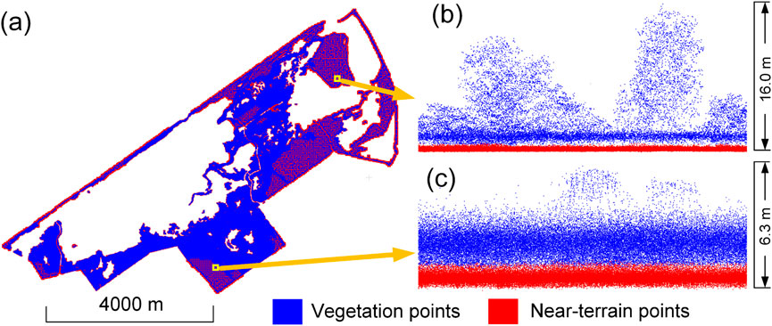
Figure 9. Near-terrain points filtering results. (a) Overview of the near-terrain points filtering result of the studied marsh area. (b and c) Side-views of two example regions as denoted by the rectangles.

4.1.3 DTM reconstruction

The DTM reconstruction used a 10 cm spatial resolution and a 30 cm radius for the elevation interpolation (Table 1). This resulted in a (near-)terrain surface for the whole marsh area (Figure 10) with a total of 155,553,656,500 grid cells. Note that the study area lies about 2–4 m below sea level (negative elevation values in Figure 10) because it is located in a polder which used to be part of an inland sea. Supplementary Figure A4 illustrates the obtained near-terrain points and the generated DTM using the presented workflow. The DTM is represented using a Triangulated Irregular Network (TIN) obtained by Delaunay triangulation. The height variation of the DTM changes when changing the radius settings (Supplementary Figure A4). DTMs obtained with a small radius showed less smoothing and more terrain details.

Figure 10

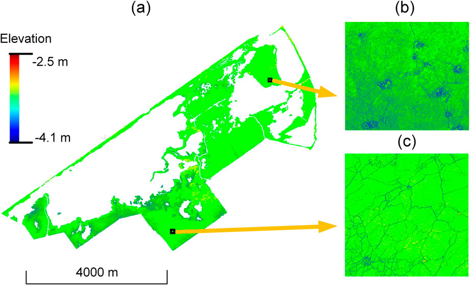
Figure 10. Generated DTM with 10 cm resolution using the obtained terrain and near-terrain points with the presented workflow. (a) DTM of the entire study area. (b and c) Top-views of the regions denoted by the rectangles. The study area lies below sea level.

4.1.4 Trail extraction

The final workflow step based on the elevation changes of DTMs from two iterations of Laplacian smoothing with a kernel size of 49 points and a $\kappa$ of 0.7 (Table 1) and the subsequent tensor voting allowed the extraction of trails for the whole marsh area (Figure 11a). The highest density of trails (darkest areas in Figure 11a) was found in the border zone with grasslands from which red deer are entering the reedbeds. For refining the “Trail” points with tensor voting (Figures 11b-d), a radius size of 1.0 m was applied with a minimum number of eight points and saliency threshold of 0.4 (Table 1). Another example of the trail extraction in the studied area is given in Supplementary Figure A5. A total area of 1.88 km² was extracted as trails, reflecting 11.6% of the 16.16 km² studied marsh area (Figure 6). Specifically, the extracted area of trails in the region of red deer grazing only, red deer and geese grazing, and geese grazing only were 0.68 km², 1.17 km², and 0.03 km², respectively. This reflected 10.46%, 12. 90%, and 4.37% of those areas.

Figure 11

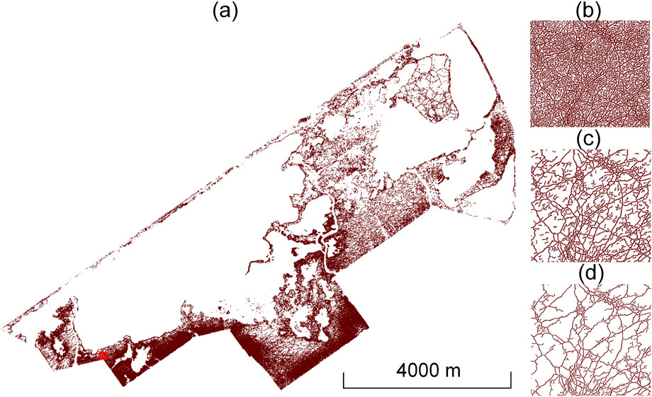
Figure 11. Extracted trails of the study area. (a) Total amount of finally extracted trails in the studied marsh area. (b) Example of trail extraction results obtained after using Laplacian smoothing. (c) Example of obtained trails after the spatial clustering algorithm had been applied. (d) Example of refined trail extraction after using sparse 3D structure tensor voting. For (b–d), the example refers to the area denoted by the red rectangle in (a).

4.1.5 Overall accuracy assessment

The accuracy assessment used the manually labelled ground truth from the sample plots (Figure 12a) and the extracted trail grid cells from the presented workflow (Figure 12b) to calculate the $Acc$. An example of one of these $30m\times 30m$ plots with a resolution of 10 cm (containing 90,000 grid cells) is shown in Figures 12a,b. For this specific sample plot, the accuracy is computed (using Equation 18) as follows:

$\text{Acc}=\frac{71016+11598}{90000}=0.92$

Figure 12

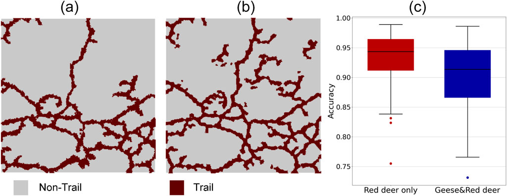
Figure 12. Accuracy of workflow for extracting red deer trails in reedbed habitat. (a and b) Example of manual versus automated trail extraction for a 30 m × 30 m sample plot, with (a) showing ground truth of red deer trails which were manually labelled by visual inspection of the point cloud, and (b) automated trail extraction results from the presented workflow in the sample plot. (c) Summary of accuracies across all sample plots, comparing areas with red deer grazing only (left, n = 50 plots) and areas where both geese and red deer are grazing (right, n = 50 plots).

Across all 50 plots in the red deer grazing only region, the overall accuracy of the automated trail extraction from the presented workflow was $Acc=0.93\pm 0.05$ (range: 0.75–0.98). For all the 50 plots in region grazed by both red deer and geese, the resulting accuracy was $Acc=0.90\pm 0.06$ (range: 0.73–0.98).

4.1.6 Sensitivity analysis

The sensitivity analyses showed how different parameter settings will influence the performance of the workflow (Figure 13). Most influential were the $Heightthreshold$, $Iteration$, $\kappa$, $R_{clustering}$, and $R_{tensor}$ (Figure 13). For the $Heighthreshold$, $\kappa$, $R_{clustering}$, and $R_{tensor}$, the overall accuracy first increases and then decreases within the range of tested parameter values. For $Iteration$, more than two iterations will smooth the features too much and thus reduce the accuracy of the trail extraction. $Kernelsize$ had a similar (but gentler) trend since it defines the size of the neighborhood that will be used to perform the smoothing step. $Minimumgridsize$, $R_{DTM}$ , Kernel size, Minimum points number, and $T_{saliency}$ had little influence on the accuracy of the trail extraction results (Figure 13). They performed best when having a low value ($Minimumgridsize$, $R_{DTM}$) or an intermediate value (Kernel size, Minimum points number, and $T_{saliency}$). The finally chosen parameter settings (indicated in red in Figure 13 and listed in Table 1) are those that provided the highest accuracy values in the 50 selected plots of the area grazed by red deer only.

Figure 13

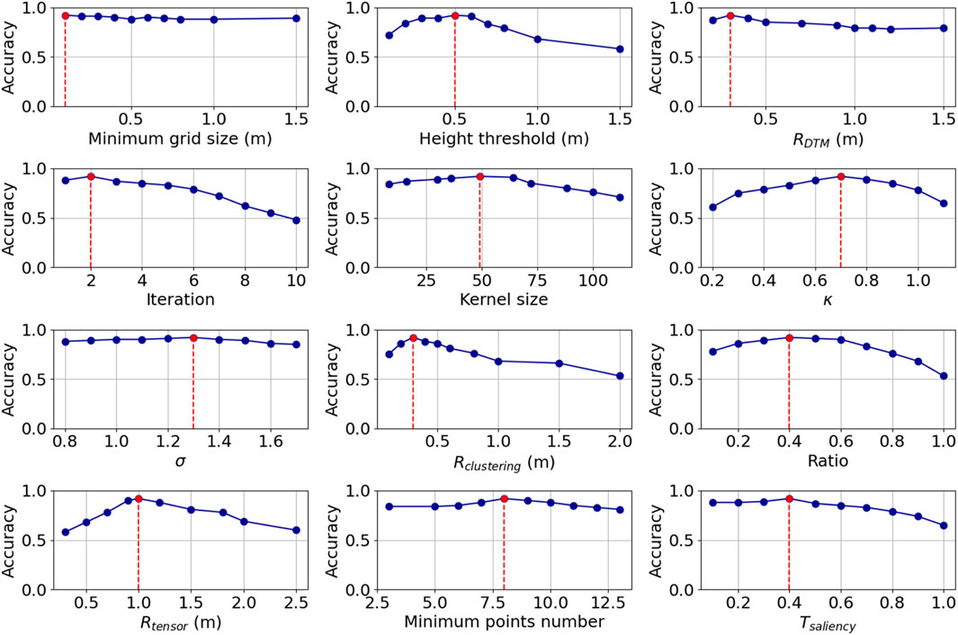
Figure 13. Sensitivity analysis showing the mean accuracy with changing parameter values across 50 sample plots from the area grazed by red deer only. The red lines and dots denote the parameters that were chosen for applying the workflow in our study area (compare Table 1).

5 Discussion

This work presents a workflow for extracting ungulate trails in wetlands using 3D point cloud data obtained from airborne laser scanning. Specifically, this work focused on reedbed habitats of the marsh area in the Oostvaardersplassen nature reserve in the Netherlands, where red deer have strongly fragmented the marsh vegetation. The workflow comprises four steps (pre-processing the raw point cloud data, filtering of near-terrain points, reconstructing DTMs, and extracting the trails using Laplacian smoothing techniques refined by sparse tensor voting). The results were validated against manually labelled datasets, demonstrating an average accuracy of 90%–93% in the study area. The sensitivity analysis allowed us to optimize the parameters in the workflow, ensuring the best performance in the study area. Overall, this workflow contributes to ecological monitoring and habitat management by offering an efficient and accurate method for assessing the impact of large herbivores such as red deer on biodiversity in marsh areas by, e.g., relating trail density to numbers of breeding birds. Below we discuss the methodological aspects of the proposed workflow, especially how the filtering of near-terrain points, the DTM generation and the trail extraction relate to other existing algorithms. We also highlight management implications and limitations of the current workflow with suggestions for future work.

5.1 Filtering of near-terrain points

Filtering near-terrain and vegetation points is a fundamental step in the proposed workflow to ensure accurate and efficient extraction of ungulate trails. The filtering process begins by taking cleaned raw ALS point clouds as input. By structuring this input into grids of multiple scales, the virtual 3D layer is iteratively refined until near-terrain points are accurately identified. Several existing filtering methods are available for segmenting terrain and vegetation points from raw ALS point clouds (Wan et al., 2018). For example, a mathematical morphology-based filtering method, which uses a moving window to perform sequential opening and closing operations, was initially proposed to separate ground and non-ground points (Lindenberger, 1993). However, this method is sensitive to fine-scale variation in terrain and vegetation points and can thus influence applications such as the extraction of ungulate trails in marsh vegetation. Applying this method to filter point clouds of marsh vegetation would result in the misclassification of vegetation points as near-terrain points, thereby introducing additional errors in the subsequent DTM reconstruction and trail extraction processes. Other algorithms have attempted to improve the overall accuracy of segmenting ground and non-ground points by incorporating additional parameters, such as slope and height threshold adaptation functions (Vosselman, 2000; Sithole, 2001; Hu et al., 2014). An example is an easy-to-use algorithm with three parameters which was proposed to simulate the terrain as a piece of cloth (Zhang et al., 2016). However, this method takes predefined fixed resolutions and is thus not very flexible. Moreover, the marsh vegetation that we studied has a relatively flat terrain, and introducing more parameters not only increases the computational effort but also provides limited improvement in overall accuracy. Some filtering algorithms first identify a proportion of ground points and then progressively expand until all points are processed. For instance, an irregular triangulated network (TIN) can be used to simulate the terrain surface, and points within a predefined distance threshold are then progressively added to the terrain points (Axelsson, 2000; Sohn and Downman, 2002). However, constructing a TIN is less efficient as it costs substantial computational time and memory. Our method using iterative 3D grid filtering is thus more efficient than other filtering methods, especially regarding two aspects. First, it only uses a proportion of the points that are within their corresponding 3D grids rather than the entire point cloud. Second, it does not require to construct a TIN and hence reduces computation time. The method we implemented for filtering of near-terrain points is therefore the most appropriate solution for our application.

5.2 DTM generation

We constructed a DTM with the obtained terrain points of the marsh habitat using an IDW interpolation method with two parameters, i.e., the resolution of the desired DTM and the radius by which the height of the DTM grid is interpolated. We predefined those two parameters based on the average point density of the used point clouds, which is 20–30 points per square meters for AHN4. Since the elevational changes in the study area are relatively small and the DTM has a high resolution (10 cm), we did not have to take additional parameters such as the local slope and roughness into account. However, if a point cloud has a lower point density compared to the desired resolution of the DTM, holes and gaps could be generated in the DTM. Other algorithms should then be considered, e.g., those that allow hole filling and more complexed elevation interpolation. An example is the thin plate spline (TPS) interpolation which combines a hierarchical multiresolution approach to construct the DTM (Mongus and Žalik, 2008). However, the accuracy of the resulting DTM can be compromised, e.g., the algorithm needs further weight adaptation if there are strong topographical changes in a study area. Another choice could be the algorithm proposed by Maguya et al. (2013) for complex terrain. This adaptive algorithm adjusts to terrain complexity by partitioning the input data and applying linear, quadratic, or cubic spline interpolation based on the characteristics of the terrain. This adaptive approach can be particularly effective in steep and forested terrains. However, the complexity of the adaptive algorithm results in higher computational demands, which can slow down the processing for large datasets. Users who apply our workflow in other study areas should therefore be aware that the steepness and complexity of the terrain can influence the DTM reconstruction.

5.3 Trail extraction

The trails created by red deer in our study area have shallow surrounding elevations and resemble the geometric shape of valleys and canals. Common methods for extracting such features from 2D grids involve the watershed delineation, which is widely used in hydrological modeling and management (Lai et al., 2016). For instance, Tarboton (1997) introduced a watershed delineation method for determining water flow directions and upslope areas in grid-based DTMs. This method calculates the flow direction as a single angle, representing the steepest downward slope from each DTM grid cell. By assigning flow between two downslope cells, this approach improves the traditional D8 (eight directions) method by reducing grid bias and minimizing dispersion. However, the method struggles to extract valleys in flat areas and water pits. By connecting local sinks using the accumulated water inflow and direction, Al-Muqdadi and Merkel (2011) addressed this challenge of watershed delineation in flat and arid terrains, where traditional methods often struggle due to low relief and poorly defined drainage patterns. However, the accuracy of their watershed delineation method heavily depends on the resolution and quality of the DTM data and involves a high computational cost. Moreover, applying their watershed delineation to the 10 cm resolution of the generated DTM in our study area would lead to a huge computational cost. Zhang et al. (2020) proposed a watershed merging algorithm designed to resolve the issue of fragmented watersheds caused by traditional delineation methods. This method merges smaller, disconnected watersheds into cohesive units based on the channel network, resulting in more realistic hydrological models. The merging process, however, is computationally expensive, especially when applied to large datasets with numerous small watersheds.

Our proposed trail extraction method uses the height residuals of two differentiated DTMs with a Laplacian smoothing technique, which has lower computational complexity and only two parameters to fine-tune the results. This potentially improves the applicability of the method and reduces computational costs but occasionally could also lead to lower accuracies. Several factors may contribute to reduced trail extraction accuracy in certain areas. First, trails with variable width or low depth may not produce sufficient elevation residuals to surpass the detection threshold, especially when the terrain is extremely flat. Second, dense or homogeneous vegetation can mask subtle terrain depressions, leading to non-classified trail grid cells. Third, variations in point cloud density or noise, such as water surface reflections, may affect interpolation quality and influence the classification of grid cells. Also, this will most likely happen if the coefficient κ is not optimal for the plots, e.g., when a large proportion of the plot area is covered by trails. We further refined the trail extraction results by employing sparse 3D structure tensor voting. The 3D stick tensor voting that we applied is a powerful technique for enhancing linear features in 3D point clouds (Laidlaw and Vilanova, 2012). It propagates local orientation information to preserve geometric continuity and emphasizes structures such as ridges, edges, and skeleton-like formations. To our knowledge, we applied this technique for the first time to extract linear ecological features. Most current applications are for medical image processing and man-made object extraction (Liu et al., 2012; Moreno et al., 2012; Soni et al., 2021). Our application could be extended to the extraction and refinement of other ecological structures such as tree lines, hedges, and stone walls. The application of sparse 3D stick tensor voting to refine the trail extraction results not only removed outliers of the obtained trail points but also allowed combining points that were located between two trail segments.

5.4 Management implications

The results from our trail extraction workflow offer insights into the habitat use of a large mammalian herbivore, in this case red deer, in vast, inaccessible and remote habitats, such as reedbeds. The results suggest that 11.6% of the marsh area is covered by red deer trails. Based on the output of the workflow, the trail density of red deer and the resulting reedbed fragmentation can be mapped using a very high (10 cm) resolution trail map. This allows ecologists and land managers to study the effects of ungulates on other species (e.g., breeding birds) and to adjust the management of large herbivores in case of negative effects. We found the highest density of trails at the edge with grasslands from which red deer are entering the reedbeds. Our study also suggests that it can be important to know which other herbivores are present in the area and affect the vegetation. In our study area, greylag geese also affect the reed vegetation as they forage on the reed leaves during moult. While doing so, they create paths starting from the open water into the reedbeds and eating the reed vegetation away alongside these paths, creating large patches of up to several ha with very low homogeneous reed vegetation that borders the water. However, the accuracy of our workflow was only slightly reduced in areas where both geese and red deer are grazing, suggesting that the effect of geese on red deer trail extraction was minor in our study area. Nevertheless, applications in other study areas should be aware that the effects of other herbivores should be taken into account.

For studying the effects of ungulate trails on the development of other species such as breeding birds, trails should be monitored over time. In the study area, it is known from annual breeding bird monitoring that some breeding bird species, e.g., the Savi’s warbler (Locustella luscinioides), appear to be in decline in areas where red deer trails are more abundant. Furthermore, visual inspection of annual aerial photographs indicate that the density of paths increased as the red deer population grew from 50 individuals in 1992 to over 3,500 individuals in 2017. After 2018, as the red deer population decreased to 900 in 2024, a visual decrease in the number of trails can be seen on the aerial photographs. However, a detailed quantitative and spatial assessment of reedbed fragmentation caused by red deer, and its effects on breeding birds, is still lacking in the study area. For effective management, it is important to understand the extent to which different herbivore densities have negative or positive impacts on nature conservation goals, such as the conservation of certain bird species. This knowledge is essential so that timely action can be taken when biodiversity begins to decline as a result of intensive grazing by ungulates. Remote sensing applications with ALS data, like the workflow we have developed here, can thus provide useful tools for habitat condition monitoring (Kissling et al., 2024).

5.5 Limitations

While the workflow presented in this study has a high accuracy in the study area and shows promising results to inform habitat management, there are a few limitations that need to be considered.

1. Transferability. This workflow has so far been developed and applied only in one study area, the Oostvaardersplassen nature reserve in the Netherlands, and with one ALS dataset (AHN4). Its transferability should be tested in other wetland areas with reedbeds, for different species of ungulates, in a variety of habitats (e.g., outside wetlands), and for ALS datasets from different time periods and with different characteristics. Certain parameter settings, such as the $Minimumgridsize$ and the $Heightthreshold$, are likely to vary depending on the used LiDAR point cloud data and the type of vegetation. $Kernelsize$ might also be related to the specific behaviour of the ungulate and its impact on vegetation structure. $R_{tensor}$ should be related to the width of the trails to ensure the linearity of a trail point in its neighbourhood can be characterized. The parameters were optimized based on the manually created ground truth using the point clouds of the study area. Those parameters probably must be re-optimized when applying the presented workflow to other study areas or datasets.

2. Computational challenges. The process is computationally intensive, requiring substantial computing power and storage capacity to handle large point cloud datasets. For instance, the tiles from the raw AHN4 point clouds used in this study have a volume of 42.3 GB. After clipping to the 36 km² large marsh area, the point clouds have a volume of 16.3 GB in LAZ format. To run the presented workflow, at least 32 GB computer memory and 40 GB storage for intermediate results and output are needed. The workflow requires specialized technical skills, including proficiency in coding (e.g., C/C++ programming, knowledge of data structures and algorithms) and knowledge of 3D LiDAR point cloud data processing. Users need to be familiar with spatial data manipulation and point cloud data processing techniques. However, it is also possible that the authors will make this workflow more accessible through converting the C++ source codes into Jupyter Notebooks using the Python programming language. This would be more friendly to users without C++ programming skills. An alternative solution would be containerization and embedding of the workflow in a virtual research environment (Kissling et al., 2024).

3. Data availability. Access to high-resolution 3D LiDAR point cloud data from ALS surveys can be a limiting factor, especially in regions where such data is unavailable or prohibitively expensive. This was not the case in our study area because all ALS point clouds of the Netherlands (including the AHN4 used here) are freely available. As an alternative, LiDAR data acquisition with Unmanned Aerial Vehicles (UAVs) is also increasingly becoming feasible, offering an additional source of spatially-explicit data for area-based conservation and land management (Kissling et al., 2024). However, the performance of the workflow to LiDAR point clouds obtained with sensors on other platforms (e.g., UAV) would then also need to be evaluated.

Addressing these limitations is essential for enhancing the robustness, transferability, and applicability of the presented workflow. Our trail extraction method could also be adapted to extract other linear features such as stone walls, hedges, and tree lines. This would make it a versatile tool for ecological applications and habitat management across diverse environments, using 3D point clouds from airborne laser scanning as an input.

6 Conclusion

This work explored the application of country-wide airborne LiDAR point cloud data to identify and map red deer trails within reedbeds of a nature reserve in the Netherlands. The developed workflow can extract these trails from 3D point clouds with high accuracy through pre-processing, filtering near-terrain points, reconstructing DTMs and employing Laplacian smoothing for trail extraction refined by sparse 3D tensor voting. The workflow allows mapping the impacts of ungulates on wetland vegetation structure and thus supports habitat management and biodiversity conservation in the study area. We recommend extending the workflow application to other regions, ungulate species and laser scanning datasets. This would allow to test the transferability of the developed method and to identify the parameter settings under a variety of ecological and environmental conditions.

Data availability statement

The original contributions presented in the study are publicly available. This data can be found here: https://doi.org/10.5281/zenodo.13889768.

Author contributions

JW: Formal Analysis, Visualization, Methodology, Validation, Software, Writing – original draft, Data curation, Writing – review and editing. PC: Writing – original draft, Writing – review and editing, Conceptualization. WDK: Investigation, Funding acquisition, Writing – original draft, Project administration, Conceptualization, Supervision, Writing – review and editing.

Funding

The author(s) declare that financial support was received for the research and/or publication of this article. This work was supported by the European Commission (MAMBO project grant number 101060639).

Acknowledgments

We acknowledge discussions with the WP4 members of the MAMBO project (https://www.mambo-project.eu/) and with members of the Biogeography and Macroecology (BIOMAC) lab at the University of Amsterdam, The Netherlands (https://www.biomac.org/).

Conflict of interest

The authors declare that the research was conducted in the absence of any commercial or financial relationships that could be construed as a potential conflict of interest.

Generative AI statement

The author(s) declare that no Generative AI was used in the creation of this manuscript.

Publisher’s note

All claims expressed in this article are solely those of the authors and do not necessarily represent those of their affiliated organizations, or those of the publisher, the editors and the reviewers. Any product that may be evaluated in this article, or claim that may be made by its manufacturer, is not guaranteed or endorsed by the publisher.

Supplementary material

The Supplementary Material for this article can be found online at: https://www.frontiersin.org/articles/10.3389/frsen.2025.1599128/full#supplementary-material

References

Al-Muqdadi, S. W., and Merkel, B. J. (2011). Automated watershed evaluation of flat terrain. J. Water Resour. Prot. 3 (12), 892–903. doi:10.4236/jwarp.2011.312099

CrossRef Full Text | Google Scholar

Alshawabkeh, Y. (2020). Linear feature extraction from point cloud using color information. Herit. Sci. 8 (1), 28. doi:10.1186/s40494-020-00371-6

CrossRef Full Text | Google Scholar

Axelsson, P. (2000). DEM generation from laser scanner data using adaptive TIN models. Int. Archives Photogrammetry Remote Sens. 33 (4), 110–117.

Google Scholar

Bakker, E. S., Veen, C. G. F., Ter Heerdt, G. J. N., Huig, N., and Sarneel, J. M. (2018). High grazing pressure of geese threatens conservation and restoration of reed belts. Front. Plant Sci. 9, 1649. doi:10.3389/fpls.2018.01649

PubMed Abstract | CrossRef Full Text | Google Scholar

Bakx, T. R., Koma, Z., Seijmonsbergen, A. C., and Kissling, W. D. (2019). Use and categorization of light detection and ranging vegetation metrics in avian diversity and species distribution research. Divers. Distributions 25 (7), 1045–1059. doi:10.1111/ddi.12915

CrossRef Full Text | Google Scholar

Bässler, C., Stadler, J., Müller, J., Förster, B., Göttlein, A., and Brandl, R. (2011). LiDAR as a rapid tool to predict forest habitat types in Natura 2000 networks. Biodivers. Conservation 20 (3), 465–481. doi:10.1007/s10531-010-9959-x

CrossRef Full Text | Google Scholar

Beemster, N., Sikkema, M., and Attema, S. (2020). Broedvogels in de moeraszone van de Oostvaardersplassen in 2019. A&W rapport 3279. Faenwalden, Netherlands: Altenburgh & Wymenga ecologisch onderzoek.

Google Scholar

Cao, K., and Zhang, X. (2020). An improved Res-UNet model for tree species classification using airborne high-resolution images. Remote Sens. 12 (7), 1128. doi:10.3390/rs12071128

CrossRef Full Text | Google Scholar

Chowdhary, C. L., and Acharjya, D. P. (2020). “Segmentation and feature extraction in medical imaging: a systematic review,” in Procedia computer science (Amsterdam, Netherlands: Elsevier B.V.), 26–36. doi:10.1016/j.procs.2020.03.179

CrossRef Full Text | Google Scholar

Cohen, L. D., and Deschamps, T. (2001). “Grouping connected components using minimal path techniques. Application to reconstruction of vessels in 2D and 3D images,” in Proceedings of the 2001 IEEE computer society conference on computer vision and pattern recognition, 2, Kauai, HI, 08-14 December, 2001. IEEE, II. doi:10.1109/CVPR.2001.990932

CrossRef Full Text | Google Scholar

Cornelissen, P. (2017). Large herbivores as a driving force of woodland-grassland cycles: the mutual interactions between the population dynamics of large herbivores and vegetation development in a eutrophic wetland. PhD, WU, Wageningen University. Wageningen University. doi:10.18174/396698

CrossRef Full Text | Google Scholar

Cornelissen, P., Jan, B., Sykora, K., and Berendse, F. (2014). Effects of large herbivores on wood pasture dynamics in a European wetland system. Basic Appl. Ecol. 15 (5), 396–406. doi:10.1016/j.baae.2014.06.006

CrossRef Full Text | Google Scholar

Daniels, J. I., Ha, L. K., Ochotta, T., and Silva, C. T. (2007). “Robust smooth feature extraction from point clouds,” in IEEE international conference on shape modeling and applications 2007 (SMI’07), 123–136.

Google Scholar

Gonzalez, S. R., Latifi, H., Weinacker, H., Dees, M., Koch, B., and Heurich, M. (2018). Integrating LiDAR and high-resolution imagery for object-based mapping of forest habitats in a heterogeneous temperate forest landscape. Int. J. Remote Sens. 39 (23), 8859–8884. doi:10.1080/01431161.2018.1500071

CrossRef Full Text | Google Scholar

Guo, X., Coops, N. C., Tompalski, P., Nielsen, S. E., Bater, C. W., and Stadt, J. J. (2017). Regional mapping of vegetation structure for biodiversity monitoring using airborne LiDAR data. Ecol. Inf. 38, 50–61. doi:10.1016/j.ecoinf.2017.01.005

CrossRef Full Text | Google Scholar

Häufel, G., Böge, M., and Bulatov, D. (2020). DTM correction in areas of steep slopes. Int. Archives Photogrammetry, Remote Sens. Spatial Inf. Sci. 43, 233–240. doi:10.5194/isprs-archives-XLIII-B2-2020-233-2020

CrossRef Full Text | Google Scholar

Hu, H., Ding, Y., Zhu, Q., Wu, B., Lin, H., Du, Z., et al. (2014). An adaptive surface filter for airborne laser scanning point clouds by means of regularization and bending energy. ISPRS J. Photogrammetry Remote Sens. 92, 98–111. doi:10.1016/j.isprsjprs.2014.02.014

CrossRef Full Text | Google Scholar

Hui, Z., Hu, Y., Jin, S., and Yevenyo, Y. Z. (2016). Road centerline extraction from airborne LiDAR point cloud based on hierarchical fusion and optimization. ISPRS J. Photogrammetry Remote Sens. 118, 22–36. doi:10.1016/j.isprsjprs.2016.04.003

CrossRef Full Text | Google Scholar

Humeau-Heurtier, A. (2019). Texture feature extraction methods: a survey. IEEE Access 7, 8975–9000. doi:10.1109/ACCESS.2018.2890743

CrossRef Full Text | Google Scholar

Jörgens, D., and Moreno, R. (2015). Tensor voting: current state, challenges and new trends in the context of medical image analysis. Math. Vis., 163–187. doi:10.1007/978-3-319-15090-1_9

CrossRef Full Text | Google Scholar

Kissling, W. D., Shi, Y., Wang, J., Walicka, A., George, C., Moeslund, J. E., et al. (2024). Towards consistently measuring and monitoring habitat condition with airborne laser scanning and unmanned aerial vehicles. Ecol. Indic. 169, 112970. doi:10.1016/j.ecolind.2024.112970

CrossRef Full Text | Google Scholar

Koma, Z., Seijmonsbergen, A. C., and Kissling, W. D. (2021a). Classifying wetland-related land cover types and habitats using fine-scale LiDAR metrics derived from country-wide airborne laser scanning. Remote Sens. Ecol. Conservation 7 (1), 80–96. doi:10.1002/rse2.170

CrossRef Full Text | Google Scholar

Koma, Z., Zlinszky, A., Bekő, L., Burai, P., Seijmonsbergen, A. C., and Kissling, W. D. (2021b). Quantifying 3D vegetation structure in wetlands using differently measured airborne laser scanning data. Ecol. Indic. 127, 107752. doi:10.1016/j.ecolind.2021.107752

CrossRef Full Text | Google Scholar

Kumar, G. N., and Mallikarjun, B. (2018). An extension to winding number and point-in-polygon algorithm. IFAC-PapersOnLine 51, 548–553. doi:10.1016/j.ifacol.2018.05.092

CrossRef Full Text | Google Scholar

Lai, Z., Li, S., Lv, G., Pan, Z., and Fei, G. (2016). Watershed delineation using hydrographic features and a DEM in plain river network region. Hydrol. Process. 30, 276–288. doi:10.1002/hyp.10612

CrossRef Full Text | Google Scholar

D. H. Laidlaw, and A. Vilanova (2012). New developments in the visualization and processing of tensor fields (Berlin, Heidelberg: Springer Science and Business Media).

Google Scholar

Lari, Z., and Habib, A. (2014). An adaptive approach for the segmentation and extraction of planar and linear/cylindrical features from laser scanning data. ISPRS J. Photogrammetry Remote Sens. 93, 192–212. doi:10.1016/j.isprsjprs.2013.12.001

CrossRef Full Text | Google Scholar

Lindenberger, J. (1993). Laser-profilmessungen zur topographischen gelandeaufnahme. Doctoral dissertation. University of Stuttgart.

Google Scholar

Lindenmayer, D., and Fischer, J. (2013). Habitat fragmentation and landscape change: an ecological and conservation synthesis. Washington: Island Press.

Google Scholar

Liu, J., and Peng, H. (2009). A method of linear feature extraction from high resolution aerial images. 6th Int. Conf. Fuzzy Syst. Knowl. Discov. FSKD 2009 3, 369–373. doi:10.1109/FSKD.2009.394

CrossRef Full Text | Google Scholar

Liu, M., Pomerleau, F., Colas, F., and Siegwart, R. (2012). “Normal estimation for pointcloud using GPU based sparse tensor voting,” in 2012 IEEE international conference on robotics and biomimetics (ROBIO) (IEEE), Guangzhou, China, 11-14 December, 2012, 91–96.

CrossRef Full Text | Google Scholar

Lucas, C., Bouten, W., Koma, Z., Kissling, W. D., and Seijmonsbergen, A. C. (2019). Identification of linear vegetation elements in a rural landscape using LiDAR point clouds. Remote Sens. 11 (3), 292. doi:10.3390/rs11030292

CrossRef Full Text | Google Scholar

Maguya, A. S., Junttila, V., and Kauranne, T. (2013). Adaptive algorithm for large scale DTM interpolation from LiDAR data for forestry applications in steep forested terrain. ISPRS J. Photogrammetry Remote Sens. 85, 74–83. doi:10.1016/j.isprsjprs.2013.08.005

CrossRef Full Text | Google Scholar

Medioni, G., Tang, C. K., and Lee, M. S. (2000). “Tensor voting: theory and applications,” in Proceedings of RFIA, 2000 Paris, France: Hermes, Lavoisier.

Google Scholar

Mongus, D., and Žalik, B. (2008). Parameter-free ground filtering of LiDAR data for automatic DTM generation. ISPRS J. Photogrammetry Remote Sens. 63 (1), 72–84. doi:10.1016/j.isprsjprs.2011.10.002

CrossRef Full Text | Google Scholar

Moreno, R., Pizarro, L., Burgeth, B., Weickert, J., Garcia, M. A., and Puig, D. (2012). “Adaptation of tensor voting to image structure estimation,” in New developments in the visualization and processing of tensor fields (Berlin Heidelberg: Springer), 29–50.

Google Scholar

Müller, A., Dahm, M., Klith Bøcher, P., Root-Bernstein, M., and Svenning, J. C. (2017). Large herbivores in novel ecosystems: habitat selection by red deer (Cervus elaphus) in a former brown-coal mining area. PLoS One 12 (5), 0177431. doi:10.1371/journal.pone.0177431

PubMed Abstract | CrossRef Full Text | Google Scholar

Nealen, A., Igarashi, T., Sorkine, O., and Alexa, M. (2006). “Laplacian mesh optimization,” in Proceedings of the 4th international conference on computer graphics and interactive techniques in Australasia and southeast Asia, GRAPHITE ’06 (New York, NY, USA: Association for Computing Machinery), 381–389. doi:10.1145/1174429.1174494

CrossRef Full Text | Google Scholar

Rusu, R. B., Marton, Z. C., Blodow, N., Dolha, M., and Beetz, M. (2008). Towards 3D point cloud-based object maps for household environments. Robotics Aut. Syst. 56 (11), 927–941. doi:10.1016/j.robot.2008.08.005

CrossRef Full Text | Google Scholar

Seitsonen, O., and Ikäheimo, J. (2021). Detecting archaeological features with airborne laser scanning in the alpine tundra of Sápmi, Northern Finland. Remote Sens. 13 (8), 1599. doi:10.3390/rs13081599

CrossRef Full Text | Google Scholar

Sithole, G. (2001). Filtering of laser altimetry data using a slope adaptive filter. Int. Archives Photogrammetry, Remote Sens. Spatial Inf. Sci. 34, 203–210.

Google Scholar

Sithole, G., and George, V. (2004). Experimental comparison of filter algorithms for bare-earth extraction from airborne laser scanning point clouds. ISPRS J. Photogrammetry Remote Sens. 59 (1–2), 85–101. doi:10.1016/j.isprsjprs.2004.05.004

CrossRef Full Text | Google Scholar

Sohn, G., and Downman, I. (2002). Terrain surface reconstruction by the use of tetrahedron model with the MDL criterion. Int. Archives Photogrammetry, Remote Sens. Spatial Inf. Sci. 36, 336–344.

Google Scholar

Soni, P. K., Rajpal, N., and Mehta, R. (2021). Road network extraction using multi-layered filtering and tensor voting from aerial images. Egypt. J. Remote Sens. Space Sci. 24 (2), 211–219. doi:10.1016/j.ejrs.2021.01.004

CrossRef Full Text | Google Scholar

Štular, B., Kokalj, Ž., Oštir, K., and Nuninger, L. (2012). Visualization of lidar-derived relief models for detection of archaeological features. J. Archaeol. Sci. 39 (11), 3354–3360. doi:10.1016/j.jas.2012.05.029

CrossRef Full Text | Google Scholar

Tarboton, D. G. (1997). A new method for the determination of flow directions and upslope areas in grid digital elevation models. Water Resour. Res. 33 (2), 309–319. doi:10.1029/96wr03137

CrossRef Full Text | Google Scholar

Thompson, A. E. (2020). Detecting classic Maya settlements with lidar-derived relief visualizations. Remote Sens. 12 (17), 2838. doi:10.3390/rs12172838

CrossRef Full Text | Google Scholar

Thuestad, A. E., Risbøl, O., Kleppe, J. I., Barlindhaug, S., and Myrvoll, E. R. (2021). Archaeological surveying of subarctic and arctic landscapes: comparing the performance of airborne laser scanning and remote sensing image data. Sustain. Switz. 13 (4), 1–19. doi:10.3390/su13041917

CrossRef Full Text | Google Scholar

Vosselman, G. (2000). Slope based filtering of laser altimetry data. Int. Archives Photogrammetry Remote Sens. 33 (Part 3B), 935–942.

Google Scholar

G. Vosselman, and H. G. Maas (2010). Airborne and terrestrial laser scanning (Boca Raton: CRC Press Taylor and Francis).

Google Scholar

Wan, P., Zhang, W., Skidmore, A. K., Qi, J., Jin, X., Yan, G., et al. (2018). A simple terrain relief index for tuning slope-related parameters of LiDAR ground filtering algorithms. ISPRS J. Photogrammetry Remote Sens. 143, 181–190. doi:10.1016/j.isprsjprs.2018.03.020

CrossRef Full Text | Google Scholar

Weinmann, M., Jutzi, B., Hinz, S., and Mallet, C. (2015). Semantic point cloud interpretation based on optimal neighborhoods, relevant features and efficient classifiers. ISPRS J. Photogrammetry Remote Sens. 105, 286–304. doi:10.1016/j.isprsjprs.2015.01.016

CrossRef Full Text | Google Scholar

Zhang, W., Qi, J., Wan, P., Wang, H., Xie, D., Wang, X., et al. (2016). An easy-to-use airborne LiDAR data filtering method based on cloth simulation. Remote Sens. 8, 501. doi:10.3390/rs8060501

CrossRef Full Text | Google Scholar

Zhang, Y., Li, W., Zhu, Y., and Ren, L. (2020). Watershed merging: a simple and effective algorithm for channel network identification and extraction. Water Resour. Res. 56 (10), e2020WR027242. doi:10.1029/2019wr026943

CrossRef Full Text | Google Scholar