Practical Data Products From Cosmic-Ray Neutron Sensing for Hydrological Applications

The Cosmic-Ray Neutron Sensor (CRNS) technique for estimating landscape average soil water content (SWC) is now a decade old and includes many practical methods for implementing measurements, such as identification of detection area and depth and determining crop biomass water equivalent. However, in order to maximize the societal relevance of CRNS SWC data, practical value-added products need to be developed that can estimate both water flux (i.e., rainfall, deep percolation, evapotranspiration) and root zone SWC changes. In particular, simple methods that can be used to estimate daily values at landscape average scales are needed by decision makers and stakeholders interested in utilizing this technique. Moreover, landscape average values are necessary for better comparisons with remote sensing products. In this work we utilize three well-established algorithms to enhance the usability of the CRNS data. The algorithms aim to: (1) temporally smooth the neutron intensity and SWC time series, (2) estimate a daily rainfall product using the Soil Moisture 2 Rain (SM2RAIN) algorithm, and (3) estimate daily root zone SWC using an exponential filter algorithm. The algorithms are tested on the CRNS site at the Hydrological Open Air Laboratory experiment in Petzenkirchen, Austria over a 3 years period. Independent observations of rainfall and point SWC data are used to calibrate the algorithms. With respect to the neutron filter, we found the Savitzky-Golay (SG) had the best results in preserving the amplitude and timing of the SWC response to rainfall as compared to the Moving Average (MA), which shifted the SWC peak by 2–4 h. With respect to daily rainfall using the SM2RAIN algorithm, we found the MA and SG filters had similar results for a range of temporal windows (3–13 h) with cumulative errors of <9% against the observations. With respect to daily root zone SWC, we found all filters behaved well (Kling-Gupta-Efficiency criteria > 0.9). A methodological framework is presented that summarizes the different processes, required data, algorithms, and products.

Introduction

The Cosmic-Ray Neutron Sensor (CRNS) is an in situ technique that is unique in its capability to estimate soil water content (SWC) at scales from ~1 to 10 ha using stationary and mobile platforms (c.f. Zreda et al., 2008, 2012; Desilets et al., 2010; Franz et al., 2015; Kohli et al., 2015; Andreasen et al., 2017). Several studies have used CRNS data to support precision agriculture (Finkenbiner et al., 2019), catchment hydrology (Fersch et al., 2018), snow hydrology (Schattan et al., 2017), land surface modeling (Rosolem et al., 2014; Baatz et al., 2017; Lawston et al., 2017), validation of remote sensing products (Montzka et al., 2017; Babaeian et al., 2018), and understanding vegetation dynamics (Franz et al., 2013). In order to maximize the societal and scientific relevance of SWC data (Vereecken et al., 2008), practical value-added products need to be developed that can estimate both water flux and root zone SWC changes. In particular, simple methods that can be used to estimate daily values at landscape average scales are needed by stakeholders as well as for better comparisons with remote sensing products (e.g., soil moisture products from Metop Advanced SCAT Scatterometer (ASCAT), NASA's Soil Moisture Active Passive mission (SMAP), ESA's Soil Moisture Ocean Salinity mission (SMOS), and Sentinel-1, see McCabe et al. (2017) for details on current and planned missions for measuring hydrologic fluxes and state variables).

While remote sensing has made significant progress in recent years (McCabe et al., 2017), significant gaps in spatial and temporal resolution and latency of images makes practical applications of retrieved hydrologic products challenging for stakeholders. For example, microwave instruments like ASCAT, SMOS, and SMAP offer a shallow (0 to ~3 cm, Jackson et al., 1997) SWC estimate at a snapshot in time and at a spatial resolution of tens of kilometers every 1–3 days. Sentinel-1 provides SWC estimates at a spatial resolution of 1 km and temporal resolution of 1.5–4 days over Europe (Bauer-Marschallingere et al., 2019). However, this is not available globally and temporal resolution of Sentinel-1 is decreased outside of Europe. Blending of different datasets can further increase the spatial and temporal resolution (e.g., SMAP and Sentinel for a 3 km product every 2–3 days). A critical and likely remaining gap for agricultural stakeholders, is providing daily field and subfield scale (0.1–10 ha) root zone SWC data (0 to ~1 m). With the inability of satellites to directly estimate root zone SWC, indirect methods using a combination of satellites, ground sensors, and models are needed to produce root zone SWC data.

The CRNS technology offers part of the solution to fill this critical measurement gap at the field scale given its ability to measure landscape average SWC over hundreds of meters horizontally and tens of centimeters vertically. Over the past decade since its development CRNS theory and best practices for equipment have greatly matured. Nonetheless, practical implementation of using the CRNS data by stakeholders requires further developing value-added products. In this methodological study, we will apply and evaluate three well-established algorithms used within the science community to increase the practical use of CRNS data. The three algorithms aim to: (1) temporally smooth the neutron intensity and SWC time series, (2) estimate a daily rainfall product using the Soil Moisture 2 Rain (SM2RAIN) algorithm (Brocca et al., 2014), and (3) estimate daily root zone SWC using an exponential filter algorithm (Wagner et al., 1999; Albergel et al., 2008). The remainder of the manuscript is organized as follows. In section Materials and methods the three algorithms will be described in detail. In section Results the algorithms will be tested on the CRNS site established in 2013 at the Hydrological Open Air Laboratory (HOAL) in Petzenkirchen, Austria (Blöschl et al., 2016) using independent observations of rainfall and a network of in situ point SWC data. Finally, in section Summary and Conclusions, we will present a summary and future recommendations.

Materials and Methods

In order to provide the reader a clear outline of the manuscript Figure 1 provides a methodological framework. The framework describes the various processes, data sources, algorithms, and value-added products covered in this study.

FIGURE 1

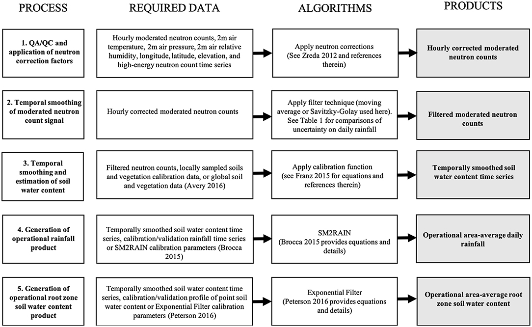
Figure 1. Methodological framework describing the different processes, required data, algorithms, and products using CRNS data from Petzenkirchen, Austria.

Study Area

A CRNS (Model # CRS 1000/B, HydroInnova LLC, Albuquerque, NM, USA) was installed at the study area in northeast Austria (48.1547°N, 15.1483°E, elevation 277 m, average slope of 8%) on 11 December 2013 and has continuously operated since (Franz et al., 2016). The study site, the Hydrological Open Air Laboratory (HOAL) (Blöschl et al., 2016), which is a cooperation project between the Federal Agency for Water Management (BAW Petzenkirchen) and the Vienna University of Technology (TU Wien), is located in Petzenkirchen, about 100 km west of Vienna. HOAL receives an annual average 823 mm of rainfall, the average annual temperature is 9.5°C, and the mean annual evapotranspiration estimated by the water balance is 628 mm/yr (1990–2014) (Blöschl et al., 2016). The research station is located in an undulating agricultural landscape, characterized by Cambisols (56%), Planosols (21%), Anthrosols (17%), Gleysols (6%), and Histosols (<1%) (United Nations, 2007). Infiltration capacities tend to be medium to low, water storage capacities tend to be high, and shrinking cracks may occur in summer due to high clay contents (Blöschl et al., 2016). The main crops are winter wheat, barley, maize, and rape. The land use at the study site consists of various parcel sizes making up a patchwork of different crops. As previously summarized by Franz et al. (2016), the location of the CRNS within the various land use parcels makes landscape average measurements of SWC challenging (Franz et al., 2016). Full details of the study site, available datasets, overarching research questions, and specific hypotheses can be found in Blöschl et al. (2016).

A network of Time-Domain Transmissivity (TDT) sensors (SPADE, Julich, Germany) were installed in the second half of 2013 and available for a portion of 2014. The TDT sensors record hourly SWC at a point and were installed at 31 sites distributed around the study area (Blöschl et al., 2016; Franz et al., 2016). At each site four TDT sensors were installed horizontally at four depths (5, 10, 20, and 50 cm). Depending on routine agricultural operations and location of the stations, 11 TDT stations were removed at various times throughout the year. In this study we only use the sensors which are located within the footprint of the CRNS. Figures 2A–D illustrates the individual TDT site time series and the large degree of spatial variation in space and time at the site. In order to compare the TDT data against the CRNS neutron data, the spatial average of each sensor depth is illustrated in Figure 2E (ignoring sensor locations with time gaps). The daily rainfall onsite is shown in Figure 2F. Lastly, weighted sums over the profile from 0–30 to 0–60 cm are computed based on sensor insertion depth. In order to compute the profile weighted averages first the arithmetic mean from all locations was computed by depth. Next a weight was assigned between the midpoint for each successive TDT sensor depth, that is a weight of 7.5 for the 5 cm sensor, 7.5 for the 10 cm probe, and 15 for the 20 cm sensor for the 0–30 cm profile average. The same process was repeated using the 50 cm sensor for the 0–60 cm profile average. The profile sums are used in this study as calibration for the exponential filter algorithm.

FIGURE 2

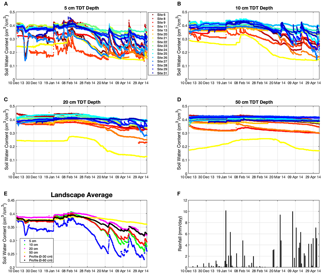
Figure 2. Time series of TDT probes organized by depth (A–D) and by site location illustrating the wide range of SWC encountered. All TDT sensors were installed in the second half of 2013 but removed over time on different dates due to the various soil cultivation and harvest times of each of the land use parcels. See Figure 2a in Franz et al. (2016) for spatial locations. (E) Time series of landscape average SWC by TDT depth and profile weighted averages of 0–30 and 0–60 cm. (F) Time series of daily rainfall data.

Temporal Filtering of CRNS Data

The CRNS technique works by counting low-energy neutrons (~0.5–1000 eV) from a moderated detector over a certain time interval (typically 1 h for stationary sensors) (see Zreda et al., 2008, 2012; Desilets et al., 2010; Andreasen et al., 2017 for details). The uncertainty of CRNS neutron count rates follows Poisson statistics (Knoll, 2000; Zreda et al., 2012), where the standard deviation is equal to the square root of the total counts. For example, 1,000 counts per hour (cph) would have an uncertainty of 31.6 cph or 3.16%. Because of the inherent counting statistics, plots of hourly neutron counts and SWC appear noisy with random fluctuations around a mean value. In order to produce a smoothed SWC time series, a temporal filter is applied to the corrected neutron data. Following the standard set of corrections for time-varying barometric pressure, high-energy incoming neutron intensity, and atmospheric water vapor (Zreda et al., 2012; Rosolem et al., 2013), a time series filter can be applied. Here we compared the 1 h corrected neutron counts vs. a Moving Average (MA) filter with different temporal windows (3–24 h) and vs. a Savitzky-Golay (SG) filter with different ordered polynomials (1st−3rd order) and temporal windows (3–25 h) (see Savitzky and Golay, 1964; Orfanidis, 1996 for full details). In general, the 1 h neutron count data had large fluctuations for this site, the MA filter is simple and widely used but the smoothed data distorted the location of the neutron trough after a rainfall event, thus affecting the timing and magnitude of the SWC peak. The SG filter was evaluated here because it is known for better balancing the degree of smoothing while minimizing the distortion of the sharp decreases/increases in the data, which is useful in preserving the amplitude and timing of neutron count decreases following a rain event. In this work we will quantify how the different neutron filter methods translate into hourly SWC, daily rainfall with the SM2RAIN algorithm and root zone SWC using the exponential filter.

Estimation of Landscape Average Rainfall Using SM2RAIN Algorithm

Given the challenge of estimating landscape average rainfall from ground based observations and top down approaches using satellites, additional sources of rainfall data are greatly needed (McCabe et al., 2017). One recently proposed approach is the Soil Moisture 2 Rain (SM2RAIN) algorithm (http://hydrology.irpi.cnr.it/research/sm2rain/ and Brocca et al., 2014; Chiaravalloti et al., 2018). SM2RAIN assumes that the soil acts like a bucket and that measurements of SWC can be inverted to estimate rainfall from a bottom up approach (Brocca et al., 2014). Following the bucket analogy the following equations can be used to describe the mass balance:

$\begin{array}{ll}{Z}^{*}\frac{ds(t)}{dt}=p(t)-r(t)-e(t)-g(t)& (1)\end{array}$

where Z^* is the soil water capacity equal to soil depth times porosity, s(t) is relative soil moisture (=SWC/porosity) as function of time t, p(t) is precipitation, r(t) is surface runoff, e(t) is evaporation, and g(t) = as(t)^b is deep drainage and a and b are calibration coefficients. During rainfall, surface runoff and evapotranspiration are assumed to be negligible at the daily timescale. This assumption will be discussed more in section Limitations of Study. Thus, precipitation can be estimated as:

$\begin{array}{ll}p(t)=Z^{*}\frac{ds(t)}{dt}+a{s(t)}^b& (2)\end{array}$

thereby leaving three parameters to calibrate (Z^*, a, b) using of observations of SWC and rainfall.

Given the wide array of SWC products at different scales the SM2RAIN algorithm has been applied and validated across time and space. By using the European Space Agency Climate Change Initiative (ESA CCI) soil moisture product, Ciabatta et al. (2018) developed a global scale SM2RAIN-CCI rainfall product that has been compared with five different global rainfall products showing good correlation at 1° spatial resolution and 5 day accumulated totals against gridded rain gauge-based rainfall observations (assumed to be the actual true rainfall). Spatial correlations range from 0.3 to 0.8 across a wide portion of the global land surface. At finer spatial (12.5 km) and temporal (1-day) resolutions, the SM2RAIN algorithm has been recently applied to the EUMETSAT Satellite Application Facility on Support to Operational Hydrology and Water Management (HSAF) soil moisture product (Brocca et al., 2019) showing better performance than a state-of-the-art satellite rainfall product (i.e., Global Precipitation Measurement, GPM) over Africa and South America. From a study in Italy, Chiaravalloti et al. (2018) compared in-situ rain gauges vs. satellite remote sensing products obtaining a correlation of around 0.7 for 24-h periods. Brocca et al. (2015) applied the SM2RAIN algorithm to in situ soil moisture observations across Europe, but the algorithm has been never applied to CRNS. Therefore, the potential of the method to obtain landscape average rainfall estimates at field scale is tested here for the first time.

Estimation of Root Zone Soil Water Content Using an Exponential Filter

A common problem with remotely sensed SWC data is that only the near surface (~0–3 cm) is directly observed using microwave wavelengths (Jackson et al., 1997). In order for these satellite products to be useful, SWC storage must be extrapolated across a plant root zone. This extrapolation can be accomplished in a number of ways using simple linear interpolation to a full data assimilation approach using a physically based water and energy balance model. However, given the computational demands, lack of boundary conditions, initial conditions, and model parameters this approach can be challenging. A fairly simple method to do root zone SWC extrapolation uses the idea of an exponential filter to solve for the time delay between surface soil response and deeper soils (Wagner et al., 1999). The exponential filter has been used with great success for remote sensing products, in-situ point scale networks (Paulik et al., 2014; Wang et al., 2017), and recently CRNS (Peterson et al., 2016).

In this study, we utilized the continuous CRNS SWC data, and assumed a depth of ~0-20 cm based on expected effective depth of the site (see Franz et al., 2012a; Kohli et al., 2015 for details on effective depth calculation). In addition, by using the seasonal TDT data from 2014 at Petzenkirchen we can parameterize the exponential filter approach, thus being able to produce an operational root zone storage product from the CRNS data henceforth. The exponential filter model considers the water balance model of a two-layer soil profile. Layer 1 has historically been set to the depth of the remote sensing product (0–3 cm) but 0–20 cm will be used here for CRNS applications. Layer 2 has been set to a root zone depth around ~1 m depending on vegetation type and local soil depths. The exponential filter approach is flexible allowing the user to specify a desired depth, given the stated assumptions about the method remain valid. Here, we will assume layer 1 is the surface layer (provided by the continuous CRNS SWC data ~0–20 cm, denoted by SWC₁), and layer 2 is the lower soil layer of interest (here an integrated root zone storage estimate constrained by the depth of the TDT sensors in order to calibrate the exponential filter approach). For demonstration purposes here a layer 2 depth of 0–30 and 0–60 cm will be provided in the following examples. Having two different root zone depths may be important to relate the available SWC with different growth stages of crop over the growing season. SWC of layer 2 (denoted by SWC₂) is described as:

$\begin{array}{ll}L\frac{dSW{C}_2}{dt}=C(SW{C}_1-SW{C}_2)& (3)\end{array}$

where t is time, L is the depth of layer 2, and C is an area-representative pseudo-diffusivity constant. This approach assumes that plant transpiration and drainage losses from the lower layer are negligible, and that hydraulic diffusivity between the soil layers is constant (Wagner et al., 1999). These limitations will be further discussed in section Limitations of Study. Equation (3) can be solved using a recursive formulation following (Albergel et al., 2008):

$\begin{array}{ll}SW{I}_{2(t)}=SW{I}_{2(t-1)}*(1-K_t)+SW{I}_{1(t)}*K_t& (4)\end{array}$

where SWI_2(t) and SWI_1(t) are the Soil Water Index (SWI) of layer 2 and layer 1, respectively, t is a time index, and K_t is the gain. Soil water index is the SWC scaled between 0 and 1 using assumed minimum and maximum values, SWI$=\left(\frac{SWC-SW{C}_{min}}{SW{C}_{max}-SW{C}_{min}}\right)$. For layer 1, the SWC is bounded by the minimum and maximum of the hourly CRNS observations. We note that the lower bound is dependent on the length of CRNS record and drier periods may be experienced in future drought periods. For layer 2, previous work has bounded SWC by the wilting point as the minimum value, and the mid-point between field capacity and porosity as the maximum value. Soil data or calibration of the model is thus required. The gain K_t ranges from 0 to 1 and is calculated as:

$\begin{array}{ll}{K}_t=\frac{K_{t-1}}{K_{t-1}+exp(-\Delta t/T)}& (5)\end{array}$

where K_t−1is the gain of the previous time step, Δt is the time step (here 1 day), and T is a characteristic time length (equal to L/C from Equation 3). The filter is initialized by setting K_t = 1 and SWI₂₍₁₎ = SWI₁₍₁₎. The characteristic time length (T) is dependent on a variety of factors, including thickness of layer 2, topographic complexity (Paulik et al., 2014), and soil properties that may influence water movement (flux) rates (Albergel et al., 2008) thus requiring local calibration. Here we followed the same methodology as Peterson et al. (2016), which calibrated three parameters, T and the layer 2 minimum and maximum SWC (T, SWC_2min, SWC_2max). In order to perform the calibration we used the in-situ TDT data and a Monte Carlo approach varying the three parameters over their expected range (SWC_2min from 0.01 to 0.25 every 0.005 cm³/cm³, SWC_2max from 0.36 to 0.75 every 0.005 cm³/cm³, and T from 10 to 70 every 2 days). The three optimal model parameters were selected based on the objective function of maximizing the Kling-Gupta-Efficiency (KGE) criteria (Gupta et al., 2009), where a perfect fit would be KGE equal to 1. KGE has been shown to be a superior metric in hydrologic model calibration (Gupta et al., 2009) as it is based on weighting the correlation, the mean, and standard deviation between the observed and predicted time series.

Results

Temporal Filtering of CRNS Data

Table 1 provides a comparison of the 24 different neutron filters propagated through the SM2RAIN algorithm for estimating daily rainfall. Using the cumulative sum percent error and KGE we selected the best MA (8 h) and SG (3rd order, 13 h) filters. These two filters and the 1 h data will be used for visual purposes for the remainder of analyses. Figure 3A illustrates the 1 h corrected neutron counts (black dots), the MA 8 h (blue dots and line) and SG 3rd order, 13 h filtered neutrons counts (red dots and line) for the Petzenkirchen site from 2013 to mid 2014 corresponding to the available TDT data. Following the neutron count filtering, the standard calibration function of Desilets et al. (2010) was applied to all datasets and SWC can be estimated, Figure 3B (see Franz et al., 2016 for on-site parameters and Supplemental Data). Figure 3C illustrates the daily liquid observed rainfall time series. Note, we also apply a porosity upper bound (=0.6 cm³/cm³ based on the sites soil bulk density, see Franz et al., 2016) to the SWC data. Neutron counts that result in SWC above porosity are due to the presence of liquid or solid water on the surface. Given the closeness of the SG and MA time series, Figure 4 provides a zoomed in view between May and June 2014. From Figures 3A, 4A the connection between rainfall events and sharp decrease in neutron count rates is evident. Also note that for periods between rainfall events a steady increase in neutron counts is observed as more water is being transported to the atmosphere and soil via evapotranspiration (soil evaporation and plant transpiration). From Figures 3, 4 it is evident that both the MA and SG filter time series follow the central tendency of the black dot data cloud. However, Figure 4B illustrates that the MA filter changes the SWC peak by 2–4 h and slightly decreases the amplitude compared to the SG filter. The change in amplitude and timing of the SWC peak will affect surface runoff generation and connections to the watershed discharge (Dingman, 2002). Here our study only focused on the connection of CRNS data to daily rainfall and root zone SWC but future work should also investigate the connections to surface runoff and discharge.

TABLE 1

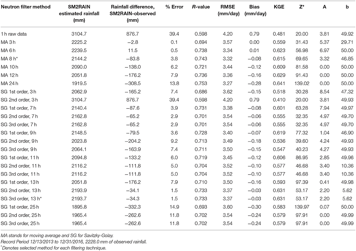
Table 1. Summary of daily rainfall error analysis using different filtering techniques on moderated neutron counts and propagating calculated SWC data through SM2RAIN algorithm.

FIGURE 3

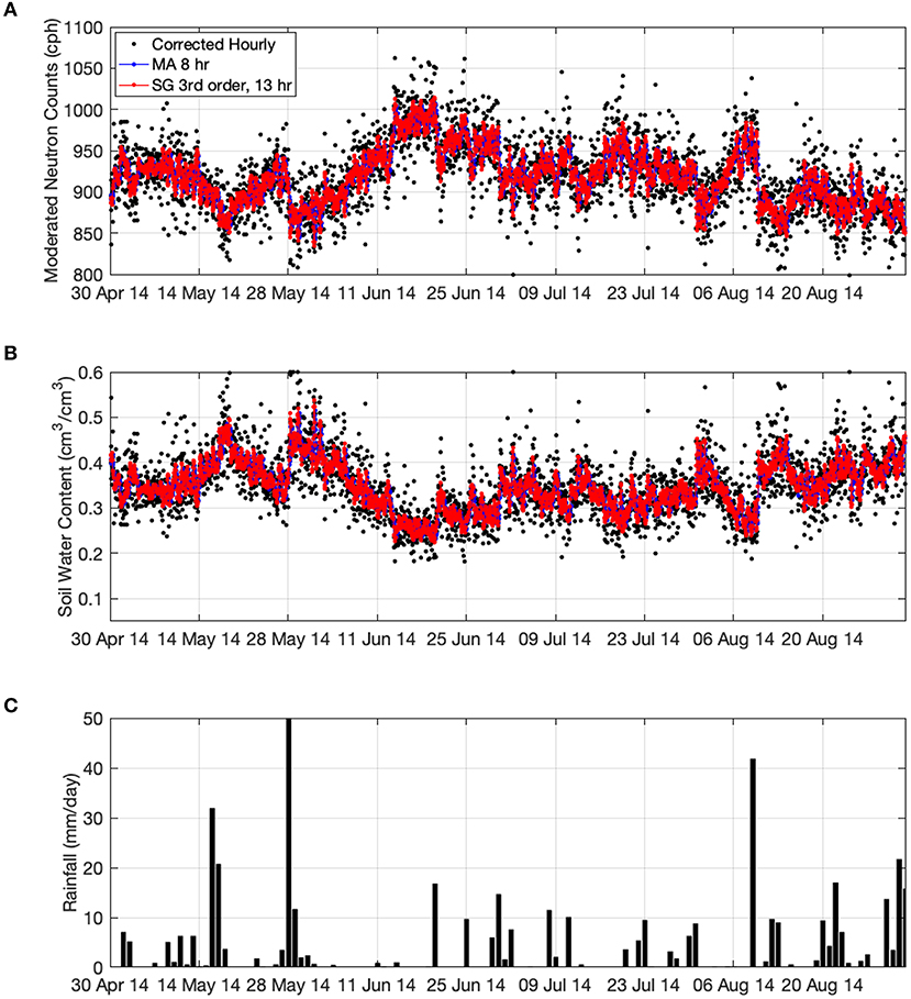
Figure 3. Time series of (A) hourly corrected neutron counts (black dots), MA (blue dots with line) and SG filtered neutrons (red dots with line), (B) hourly SWC using the Desilets et al. (2010) equation and (C) daily rainfall observed study site for the same time period as TDT observations.

FIGURE 4

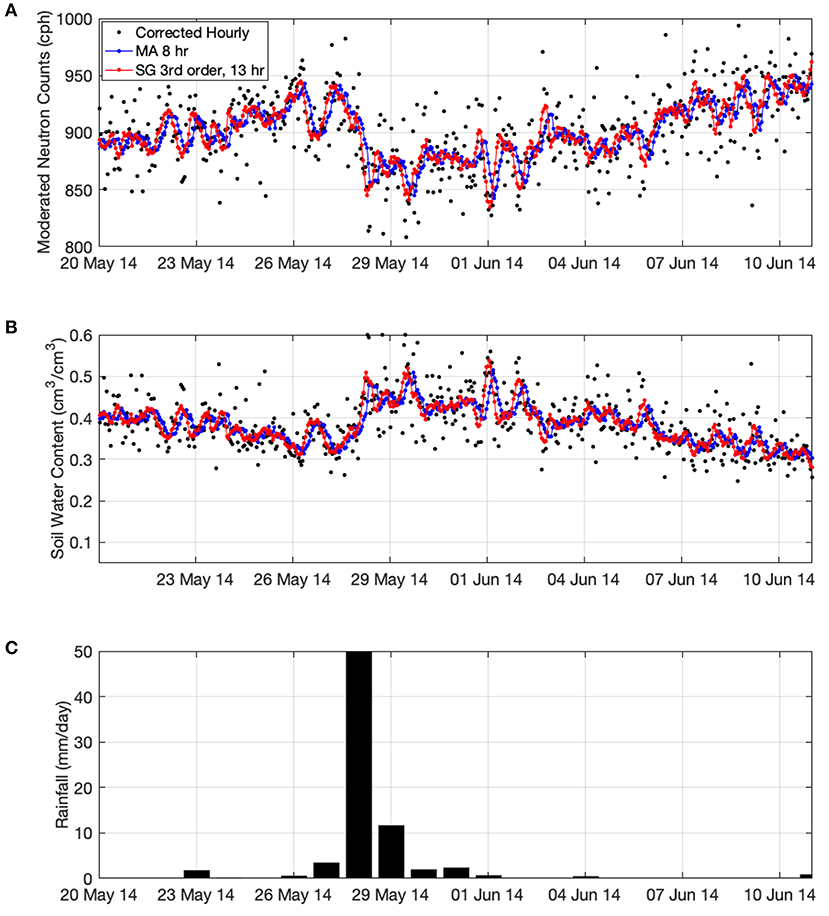
Figure 4. Zoomed in times series of Figure 3 better illustrating the 2–4 h shift in the timing of rainfall using the MA filter the Petzenkirchen. (A) Hourly corrected neutron counts (black dots), MA (blue dots with line) and SG filtered neutrons (red dots with line), (B) hourly SWC using the Desilets et al. (2010) equation and (C) daily rainfall observed study site for the same time period.

Estimation of Landscape Average Rainfall Using SM2RAIN Algorithm

Table 1 summarizes the 24 different neutron filters using the SM2RAIN algorithm and rain gauge observations at Petzenkirchen. The rainfall observations are used to select the three free parameters (Z^*, a, b) in Equation (2) by minimizing the root mean square error (RMSE) between observed and estimated daily rainfall. The 1 h data results in a poor comparison with the observed data as the cumulative sum is 39.4% larger than the observations (3104.7 vs. 2,228 mm over the 3 year period, 2013–2016). The MA filter with a temporal window of 3–12 h resulted in small cumulative error (<8%). The SG filter with 1st−3rd order polynomials and temporal windows of 7–13 h also had small cumulative error (<9%). The other statistical metrics (Pearson correlation (R), KGE, Bias) were also comparable for these neutron filters.

Comparing the three parameters with Brocca et al. (2015) we find different values. This is expected as the CRNS depth and remote sensing depths are different (~20 vs. 3 cm). At the daily level, a R-value of 0.74 and 0.73 is found for the study site for the optimal MA and SG filters, which is comparable with the results obtained with satellite soil moisture products (e.g., Chiaravalloti et al., 2018; Brocca et al., 2019). Figure 5 illustrates the daily cumulative sum of the three selected filters vs. the observed rainfall, again showing excellent agreement for the SG and MA filters. There are a few periods early in the record that show small deviations. If compared with the results obtained with classical in situ measurements shown in Brocca et al. (2015), in which the range of R-values is between 0.75 and 0.95, the performance with CRNS SWC are in the lower range but with the significant added-value to provide landscape average rainfall estimates. Table 2 includes summary statistics for rainfall accumulations of 1, 3, and 5 days. For increasing integration time the statistical metrics improve to levels reported by Brocca et al. (2015) and Chiaravalloti et al. (2018). With respect to error the World Meteorological Organization (De Valle et al., 2007 and https://www.wmo-sat.info/oscar/variables/view/1) reports rain gage error around 1 and 2–4 mm/day for satellite estimates, however each method has different spatial resolution and coverage. The CRNS derived rainfall provides a missing and critical gap at the 1–10 ha scale.

FIGURE 5

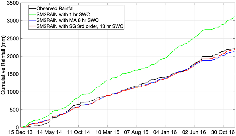
Figure 5. Cumulative sums of observed rainfall and SM2RAIN estimates using three neutron filters. See Table 1 for full summary.

TABLE 2

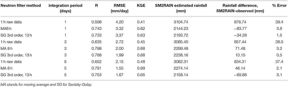
Table 2. Summary of SM2RAIN algorithm statistical performance at Petzenkirchen for different integration periods.

Estimation of Root Zone Soil Water Content Using an Exponential Filter

Figure 2E illustrates the time series of landscape average TDT sensors by depth that were available at the HOAL from 2013 to 2014. Due to various land management operations the sensors were removed from different land uses at different times. In order to calibrate the exponential filter model to a root zone product a profile SWC was estimated from a weighted average of TDT sensors within those 0–30 and 0–60 cm profiles. Using the CRNS SWC data as layer 1 and the SWC profile 0–30 and 0–60 cm data as layer 2, the three free parameters for the exponential filter model (Equations 3, 4) were estimated using a Monte Carlo approach. The objective function was maximizing KGE between the observed and modeled SWC time series. Table 3 provides the summary results illustrating that all three methods had large KGE values of >0.9. Estimates of SWC_2max and T were very similar for all methods. SWC_1min was lower for the 1 h neutron data due to the higher random fluctuations. As expected T was larger for the 0–60 cm layer. Following calibration Figures 6A,B illustrate the comparison of SWC between the exponential filter fit and the TDT landscape averages for both depths. With respect to estimating the critical parameter T, Paulik et al. (2014) used the International Soil Moisture Network (Dorigo et al., 2013) data to compare T vs. different environmental covariates. Paulik et al. (2014) found depth and topographic complexity were most correlated to T. In contrast, Wang et al. (2017) used the Nebraska Mesonet sites (same sensor type) and found that T was strongly correlated to depth and soil texture (percent sand and clay). We note that a relatively new commercial product exists that uses the exponential filter with a combination of passive microwave sensors to produce an operational daily 100 m SWC product at 10, 20, and 40 cm (https://www.vandersat.com/soil-moisture-monitoring).

TABLE 3

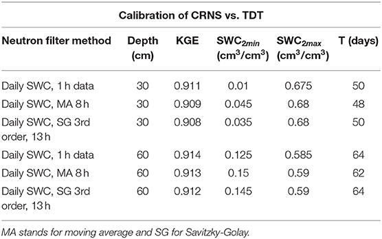
Table 3. Summary of calibration fit and three parameter estimates for the 0–30 and 0–60 cm exponential filter models for different neutron filters.

FIGURE 6

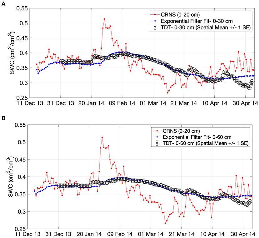
Figure 6. Comparison of SWC for the CRNS (neutron filter SG 3rd order, 13 h), fitted exponential model, and observed landscape average TDT data for the (A) 0–30 cm and (B) 0–60 cm products.

Using the CNRS SWC data and the exponential model fits in Table 3 an operational daily SWC product for 0–30 and 0–60 cm can be produced. Figure 7 illustrates the CRNS SWC, 0–30 cm SWC, and 0–60 cm SWC products. By tracking changes in SWC over these depths in real-time stakeholders will be able to make more informed decisions about irrigation, fertilization rates, and other management operations.

FIGURE 7

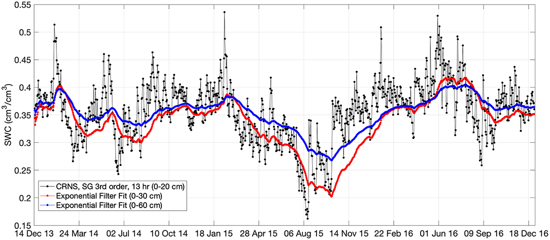
Figure 7. Time series of SWC for CRNS, 0–30 cm exponential filter product, and 0–60 cm exponential filter product for the 3 years period.

Limitations of Study

The key limitation of this work is that only a single CRNS site was used, mainly due to the challenge of having a high-density in-situ SWC network to calibrate the algorithms. Several other studies have such networks (e.g., Franz et al., 2012a,b; Bogena et al., 2013; Lv et al., 2014) and would be good candidates to validate and extend this work. Another limitation of this work is that the optimal filter window for the MA and SG methods is dependent on the total counts, which are related to the site location (i.e., geomagnetic latitude), elevation, and detector size/type. We anticipate the optimal window size will decrease with increased total counts. This is important for use of the MA filter, particularly in minimizing any shifts in timing or amplitude of the SWC peak following a rain event. Accurate depiction of the SWC peak is critical for understanding the connection between CRNS data and surface runoff and discharge. This topic was beyond the scope of the current study but deserves more attention in the future.

With respect to the SM2RAIN algorithm, the CRNS data performed comparable to rain gage and satellite products for the MA and SG neutron filters. The 1 h data lead to a 39.4% overestimation of rainfall due to the random fluctuations in the neutron counts. The key assumption for the SM2RAIN method is that no surface runoff is generated during rainfall, which may be violated for certain sites. In addition, selection of the three parameters did vary with choice of neutron filter algorithm. Current versions of the SM2RAIN algorithm do include a self-calibration procedure. We did find that adding the criteria of cumulative sum percent error against the observed rainfall was helpful in selecting appropriate window sizes for evaluating the filters and conserving water mass balance.

With respect to daily root zone SWC, all three neutron filtering techniques worked well, albeit the 1 h data had a different SWC_2min parameter. The main challenge of the exponential filter approach is selection of the T parameter for novel sites where in-situ data may be unavailable. Paulik et al. (2014) found using the ISMN SWC data that depth and topographic complexity were most correlated to T, whereas Wang et al. (2017) found T was highly correlated to depth and soil texture for the Nebraska Mesonet site data. What is clear is that caution should be used when applying the exponential filter approach for sites with shallow water tables, large topographic relief, and dense vegetation. Given these limitations, the method's simplicity and widespread operational use in remote sensing and commercial products make it a viable candidate for extending the use of CRNS SWC data.

Summary and Conclusions

This methodological paper provides the background, equations, and example calculations from the Petzenkirchen CRNS study site using three well-established algorithms summarized in the methodological framework in Figure 1 and available for general use (see Data Availability Statement). The algorithms make the essential step of enhancing the CRNS SWC data for providing stakeholders with the value-added products of a smoothed SWC time series, landscape average rainfall, and root zone SWC data in order to make decisions. While the provided examples are written in the computer program MATLAB R2018b mostly used by engineers and academics, next steps require the data and value-added products and code be made available on web-based data portals, code sharing environments and smartphone applications for use by stakeholders. Therefore, this paper serves as a critical but only a first step toward adoption of CRNS data toward practical applications. Future work with CRNS and available in situ SWC data should further validate these approaches and their use in complex environments.

Data Availability Statement

The datasets generated for this study can be found in the Mendeley Repository with the citation- Franz, Trenton (2020), Data for Cosmic-Ray Neutron Sensor: Practical Data Products from Cosmic-Ray Neutron Sensing for Hydrological Applications, Mendeley Data, V2, doi: 10.17632/cxzjjm2txx.2. The neutron intensity smoothing and exponential filter code written in MATLAB R2018b are available upon written request to the corresponding author (tfranz2@unl.edu). The SM2RAIN code is available from LB at http://hydrology.irpi.cnr.it/research/sm2rain/ for a variety of platforms.

Author Contributions

TF performed the primary data analysis and wrote the manuscript. AW and JZ assisted with data analysis and edited the manuscript. LH and GD provided funding, laboratory access, and edited the manuscript. PS and MV provided datasets from HOAL and edited the manuscript. LB provided access to SM2RAIN algorithm, assisted with data analysis, and edited the manuscript. WW edited the manuscript.

Funding

Financial support was provided by the Joint FAO/IAEA Programme of Nuclear Techniques in Food and Agriculture through the Coordinated Research Project (CRP) D1.50.17 Nuclear Techniques for a Better Understanding of the Impact of Climate Change on Soil Erosion in Upland Agro ecosystems (2015–2020) and CRP D1.20.14 Enhancing agricultural resilience and water security using Cosmic-Ray Neutron Sensor (2019–2024).

Conflict of Interest

The authors declare that the research was conducted in the absence of any commercial or financial relationships that could be construed as a potential conflict of interest.

Acknowledgments

The authors would like to acknowledge the support of the Hydrological Open Air Laboratory, the Soil and Water Management & Crop Nutrition Laboratory of the Joint Division of Nuclear Techniques in Food and Agriculture, the Vienna Doctoral Programme on Water Resources Systems and Georg Weltin in the installation and maintenance of the CRNS.

Supplementary Material

The Supplementary Material for this article can be found online at: https://www.frontiersin.org/articles/10.3389/frwa.2020.00009/full#supplementary-material

Supplemental Data. Containing the raw and processed data.

References

Albergel, C., Rudiger, C., Pellarin, T., Calvet, J. C., Fritz, N., Roissard, R., et al. (2008). From near-surface to root-zone soil moisture using an exponential filter: an assessment of the method based on in-situ observations and model simulations. Hydrol. Earth Syst. Sci. 12, 1323–1337. doi: 10.5194/hess-12-1323-2008

CrossRef Full Text | Google Scholar

Andreasen, M., Jensen, K. H., Desilets, D., Franz, T., Zreda, M., Bogena, H. R., et al. (2017). Status and perspectives on the cosmic-ray neutron method for soil moisture estimation and other environmental science applications. Vadose Zone J. 16:11. doi: 10.2136/vzj2017.04.0086

CrossRef Full Text | Google Scholar

Avery, W., Finkenbiner, C., Franz, T. E., Wang, T., Nguy-Roberston, A., Arkebauer, T., et al. (2016). Incorporation of globally available datasets into the roving cosmic-ray neutron probe method for estimating field-scale soil water content. Hydrol. Earth Syst. Sci. Discuss. 20, 3859–3872. doi: 10.5194/hess-20-3859-2016

CrossRef Full Text | Google Scholar

Baatz, R., Franssen, H. J. H., Han, X., Hoar, T., Vereecken, H., Bogena, H. R., et al. (2017). Evaluation of a cosmic-ray neutron sensor network for improved land surface model prediction. Hydrol. Earth Syst. Sci. 21, 2509–2530. doi: 10.5194/hess-21-2509-2017

CrossRef Full Text | Google Scholar

Babaeian, E., Sadeghi, M., Franz, T. E., Jones, S., and Tuller, M. (2018). Mapping soil moisture with the OPtical TRApezoid Model (OPTRAM) based on long-term MODIS observations. Remote Sens. Environ. 211, 425–440. doi: 10.1016/j.rse.2018.04.029

CrossRef Full Text | Google Scholar

Bauer-Marschallingere, B., Freeman, V., Cao, S., Paulik, C., Schaufler, S., Stachl, T., et al. (2019). Toward global soil moisture monitoring with sentinel-1: harnessing assets and overcoming obstacles. IEEE Trans. Geosci. Remote Sens. 57, 520–539. doi: 10.1109/TGRS.2018.2858004

CrossRef Full Text | Google Scholar

Blöschl, G., Blaschke, A. P., Broer, M., Bucher, C., Carr, G., Chen, X., et al. (2016). The Hydrological Open Air Laboratory (HOAL) in Petzenkirchen: a hypotheses-driven observatory. Hydrol. Earth Syst. Sci. 20, 227–255. doi: 10.5194/hess-20-227-2016

CrossRef Full Text | Google Scholar

Bogena, H. R., Huisman, J. A., Baatz, R., and Franssen, H. J. H. (2013). Accuracy of the cosmic-ray soil water content probe in humid forest ecosystems: the worst case scenario. Water Resour. Res. 49, 5778–5791. doi: 10.1002/wrcr.20463

CrossRef Full Text | Google Scholar

Brocca, L., Ciabatta, L., Massari, C., Moramarco, T., Hahn, S., Hasenauer, S., et al. (2014). Soil as a natural rain gauge: estimating global rainfall from satellite soil moisture data. J. Geophys. Res. Atmos. 119, 5128–5141. doi: 10.1002/2014JD021489

CrossRef Full Text | Google Scholar

Brocca, L., Filippucci, P., Hahn, S., Ciabatta, L., Massari, C., Camici, S., et al. (2019). SM2RAIN-ASCAT (2007-2018): global daily satellite rainfall from ASCAT soil moisture. Earth Syst. Sci. Data 11, 1583–1601. doi: 10.5194/essd-11-1583-2019

CrossRef Full Text | Google Scholar

Brocca, L., Massari, C., Ciabatta, L., Moramarco, T., Penna, D., Zuecco, G., et al. (2015). Rainfall estimation from in situ soil moisture observations at several sites in Europe: an evaluation of SM2RAIN algorithm. J. Hydrol. Hydromech. 63, 201–209. doi: 10.1515/johh-2015-0016

CrossRef Full Text | Google Scholar

Chiaravalloti, F., Brocca, L., Procopio, A., Massari, C., and Gabriele, S. (2018). Assessment of GPM and SM2RAIN-ASCAT rainfall products over complex terrain in southern Italy. Atmos. Res. 206, 64–74. doi: 10.1016/j.atmosres.2018.02.019

CrossRef Full Text | Google Scholar

Ciabatta, L., Massari, C., Brocca, L., Gruber, A., Reimer, C., Hahn, S., et al. (2018). SM2RAIN-CCI: a new global long-term rainfall data set derived from ESA CCI soil moisture. Earth Syst. Sci. Data 10, 267–280. doi: 10.5194/essd-10-267-2018

CrossRef Full Text | Google Scholar

De Valle, V., Vuerich, E., Monesi, C., Lanza, L. G., Stagi, L., and Lanzinger, E. (2007). WMO Field Intercomparison of Rainfall Intensity Gauges. World Meteorological Organization instruments and observing methods report no. 99. Geneva: World Meteorological Organization.

Google Scholar

Desilets, D., Zreda, M., and Ferre, T. P. A. (2010). Nature's neutron probe: land surface hydrology at an elusive scale with cosmic rays. Water Resour. Res. 46:W11505. doi: 10.1029/2009WR008726

CrossRef Full Text | Google Scholar

Dingman, L. S. (2002). Physical Hydrology, 2ndEdn. Upper Saddle River, NJ: Prentice-Hall Inc.

Google Scholar

Dorigo, W. A., Xaver, A., Vreugdenhil, M., Gruber, A., Hegyiova, A., Sanchis-Dufau, A., et al. (2013). Global automated quality control of in situ oil moisture data from the international soil moisture network. Vadose Zone J. 12:21. doi: 10.2136/vzj2012.0097

CrossRef Full Text | Google Scholar

Fersch, B., Jagdhuber, T., Schron, M., Volksch, I., and Jager, M. (2018). Synergies for soil moisture retrieval across scales from airborne polarimetric SAR cosmic ray neutron roving, and an in situ sensor network. Water Resour. Res. 54, 9364–9383. doi: 10.1029/2018WR023337

CrossRef Full Text | Google Scholar

Finkenbiner, C. E., Franz, T. E., Gibson, J., Heeren, D. M., and Luck, J. (2019). Integration of hydrogeophysical datasets and empirical orthogonal functions for improved irrigation water management. Precis. Agric. 20, 78–100. doi: 10.1007/s11119-018-9582-5

CrossRef Full Text | Google Scholar

Franz, T. E., Wahbi, A., Vreugdenhil, M., Weltin, G., Heng, L., Oismueller, M., et al. (2016). Using cosmic-ray neutron probes to monitor landscape scale soil water content in mixed land use agricultural systems. Appl. Environ. Soil Sci. 2016:1–11. doi: 10.1155/2016/4323742

CrossRef Full Text | Google Scholar

Franz, T. E., Wang, T., Avery, W., Finkenbiner, C., and Brocca, L. (2015). Combined analysis of soil moisture measurements from roving and fixed cosmic ray neutron probes for multiscale real-time monitoring. Geophys. Res. Lett. 42, 3389–3396. doi: 10.1002/2015GL063963

CrossRef Full Text | Google Scholar

Franz, T. E., Zreda, M., Ferre, P. A., Rosolem, R., Zweck, C., Stillman, S., et al. (2012a). Measurement depth of the cosmic-ray soil moisture probe affected by hydrogen from various sources. Water Resour. Res. 48:8515. doi: 10.1029/2012WR011871

CrossRef Full Text | Google Scholar

Franz, T. E., Zreda, M., Rosolem, R., and Ferre, P. A. (2012b). Field validation of cosmic-ray soil moisture sensor using a distributed sensor network. Vadose Zone J. 11. doi: 10.2136/vzj2012.0046

CrossRef Full Text | Google Scholar

Franz, T. E., Zreda, M., Rosolem, R., Hornbuckle, B., Irvin, S., Adams, H., et al. (2013). Ecosystem scale measurements of biomass water using cosmic-ray neutrons. Geophys. Res. Lett. 40, 3929–3933. doi: 10.1002/grl.50791

CrossRef Full Text | Google Scholar

Gupta, H. V., Kling, H., Yilmaz, K. K., and Martinez, G. F. (2009). Decomposition of the mean squared error and NSE performance criteria: implications for improving hydrological modelling. J. Hydrol. 377, 80–91. doi: 10.1016/j.jhydrol.2009.08.003

CrossRef Full Text | Google Scholar

Jackson, T. J., Oneill, P. E., and Swift, C. T. (1997). Passive microwave observation of diurnal surface soil moisture. IEEE Trans. Geosci. Remote Sens. 35, 1210–1222. doi: 10.1109/36.628788

CrossRef Full Text | Google Scholar

Knoll, G. F. (2000). Radiation Detection and Measurement. Hoboken, NJ: John Wiley & Sons, Inc.

Google Scholar

Kohli, M., Schron, M., Zreda, M., Schmidt, U., Dietrich, P., and Zacharias, S. (2015). Footprint characteristics revised for field-scale soil moisture monitoring with cosmic-ray neutrons. Water Resour. Res. 51, 5772–5790. doi: 10.1002/2015WR017169

CrossRef Full Text | Google Scholar

Lawston, P. M., Santanello, J. A., Franz, T. E., and Rodell, M. (2017). Assessment of irrigation physics in a land surface modeling framework using non-traditional and human-practice datasets. Hydrol. Earth Syst. Sci. 21, 2953–2966. doi: 10.5194/hess-21-2953-2017

PubMed Abstract | CrossRef Full Text | Google Scholar

Lv, L., Franz, T. E., Robinson, D. A., and Jones, S. (2014). Measured and mpodeled soil moisture compared with cosmic-ray neutron robe estimates in a mixed forest. Vadose Zone J. 13:13. doi: 10.2136/vzj2014.06.0077

CrossRef Full Text | Google Scholar

McCabe, M. F., Rodell, M., Alsdorf, D. E., Miralles, D. G., Uijlenhoet, R., Wagner, W., et al. (2017). The future of earth observation in hydrology. Hydrol. Earth Syst. Sci. 21, 3879–3914. doi: 10.5194/hess-21-3879-2017

PubMed Abstract | CrossRef Full Text | Google Scholar

Montzka, C., Bogena, H. R., Zreda, M., Monerris, A., Morrison, R., Muddu, S., et al. (2017). Validation of spaceborne and modelled surface soil moisture products with cosmic-ray neutron probes. Remote Sens. 9:103. doi: 10.3390/rs9020103

CrossRef Full Text | Google Scholar

Orfanidis, S. J. (1996). Introduction to Signal Processing. Englewood Cliffs, NJ: Prentice-Hall.

Google Scholar

Paulik, C., Dorigo, W., Wagner, W., and Kidd, R. (2014). Validation of the ASCAT Soil Water Index using in situ data from the International Soil Moisture Network. Int. J. Appl. Earth Obs. Geoinf. 30, 1–8. doi: 10.1016/j.jag.2014.01.007

CrossRef Full Text | Google Scholar

Peterson, A. M., Helgason, W. D., and Ireson, A. M. (2016). Estimating field-scale root zone soil moisture using the cosmic-ray neutron probe. Hydrol. Earth Syst. Sci. 20, 1373–1385. doi: 10.5194/hess-20-1373-2016

CrossRef Full Text | Google Scholar

Rosolem, R., Hoar, T., Arellano, A., Anderson, J. L., Shuttleworth, W., Zeng, X., et al. (2014). Translating aboveground cosmic-ray neutron intensity to high-frequency soil moisture profiles at sub-kilometer scale. Hydrol. Earth Syst. Sci. 18, 4363–4379. doi: 10.5194/hess-18-4363-2014

CrossRef Full Text | Google Scholar

Rosolem, R., Shuttleworth, W. J., Zreda, M., Franz, T. E., Zeng, X., Papuga, S., et al. (2013). The effect of atmospheric water vapor on the cosmic-ray soil moisture signal. J. Hydrometeorol. 14, 1659–1671. doi: 10.1175/JHM-D-12-0120.1

CrossRef Full Text | Google Scholar

Savitzky, A., and Golay, M. J. E. (1964). Smoothing and differentiation of data by simplified least square procedure. Anal. Chem. 36, 1627–1639. doi: 10.1021/ac60214a047

CrossRef Full Text | Google Scholar

Schattan, P., Baroni, G., Oswald, S. E., Schober, J., Fey, C., Kormann, C., et al. (2017). Continuous monitoring of snowpack dynamics in alpine terrain by aboveground neutron sensing. Water Resour. Res. 53, 3615–3634. doi: 10.1002/2016WR020234

CrossRef Full Text | Google Scholar

United Nations (2007). World Reference Base for Soil Resources 2006. World Soil Resources Reports No. 103. United Nations Food and Agriculture Organization, IUSS Working Group WRB, FAO, Rome. Available online at: http://www.fao.org/fileadmin/templates/nr/images/resources/pdf_documents/

Google Scholar

Vereecken, H., Huisman, J. A., Bogena, H., Vanderborght, J., Vrugt, J., Hopmans, J. W., et al. (2008). On the value of soil moisture measurements in vadose zone hydrology: a review. Water Resour. Res. 44:W00D06. doi: 10.1029/2008WR006829

CrossRef Full Text | Google Scholar

Wagner, W., Lemoine, G., and Rott, H. (1999). A method for estimating soil moisture from ERS scatterometer and soil data. Remote Sens. Environ. 70, 191–207. doi: 10.1016/S0034-4257(99)00036-X

CrossRef Full Text | Google Scholar

Wang, T. J., Franz, T. E., You, J. S., Shulski, M., and Ray, C. (2017). Evaluating controls of soil properties and climatic conditions on the use of an exponential filter for converting near surface to root zone soil moisture contents. J. Hydrol. 548, 683–696. doi: 10.1016/j.jhydrol.2017.03.055

CrossRef Full Text | Google Scholar

Zreda, M., Desilets, D., Ferre, T. P. A., and Scott, R. L. (2008). Measuring soil moisture content non-invasively at intermediate spatial scale using cosmic-ray neutrons. Geophys. Res. Lett. 35:L21402. doi: 10.1029/2008GL035655

CrossRef Full Text | Google Scholar

Zreda, M., Shuttleworth, W. J., Xeng, X., Zweck, C., Desilets, D., Franz, T., et al. (2012). COSMOS: the COsmic-ray soil moisture observing system. Hydrol. Earth Syst. Sci. 16, 4079–4099. doi: 10.5194/hess-16-4079-2012

CrossRef Full Text | Google Scholar