Relative Impacts of Projected Climate and Land Use Changes on Terrestrial Water Balance: A Case Study on Ganga River Basin

Saha, Anamitra; Ghosh, Subimal

doi:10.3389/frwa.2020.00012

ORIGINAL RESEARCH article

Front. Water, 11 June 2020

Sec. Water and Built Environment

Volume 2 - 2020 | https://doi.org/10.3389/frwa.2020.00012

This article is part of the Research Topic Past, Present, and Future Impacts of Climate on Infrastructure View all 7 articles

Relative Impacts of Projected Climate and Land Use Changes on Terrestrial Water Balance: A Case Study on Ganga River Basin

$\nAnamitra Saha$ Anamitra Saha¹

Subimal Ghosh^1,2^*

¹Department of Civil Engineering, Indian Institute of Technology Bombay, Mumbai, India
²Interdisciplinary Program in Climate Studies, Indian Institute of Technology Bombay, Mumbai, India

The Ganga river basin, being one of the largest river basins in South-East Asia, with area over 1 million Km² and population over 400 million, is highly vulnerable to water scarcity due to climate change and rapid growth in agriculture, industrialization, and urbanization. To understand the potential impact of climate and land use changes on regional terrestrial water balance has become crucial for ensuring appropriate water management strategies for adaptation and mitigation purposes. In this study we employ an RCP-SSP (Representative Concentration Pathways—Shared Socioeconomic Pathways) scenario framework (1.5 and 2°C warming scenarios and SSP1–5) to explore the relative impacts of projected twenty-first century climate and land use changes on the surface hydrology of the Ganga river basin. By statistically comparing the hydrological responses of each combination of socioeconomic and climate mitigation pathways against a control scenario, we distinguish between the impacts of each scenario. We also analyze our data in a conceptual framework to understand how climatic and land use factors impact the basin characteristics and which one among them is projected to be the dominant factor in our study region. Our results show that, in terms of hydrologic impact assessment, climate change mitigation pathways are the dominant factor and the land use changes associated with socio-economic pathways contribute little to the projected future changes.

Introduction

India has a population of more than 1.3 billion, which is around 17% of the world's population, but only 1,121 Km³ of estimated utilizable water resources, about 4% of global freshwater resources [Central Water Commission (CWC), 2013; United Nations (UN), 2019]. In the last few decades the country has experienced a continuous rise in population along with economic growth and increased food, energy, and water consumption [Global Water Partnership (GWP), 2013]. Rapid growth in agriculture, industrialization, and urbanization has led to increasing demand for freshwater throughout the country. In terms of water usage, agriculture is the dominating sector, with about 80% share of the total water demand (Bhat, 2014). The water availability and the agricultural and economic productivity of India are heavily dependent on the south-west monsoon (Krishna Kumar et al., 2004; Gadgil and Gadgil, 2006). More than 80% of annual rainfall in India occurs during the monsoon months (June-September, JJAS), which totals to 904 mm on average, compared to 294 mm of rainfall during the rest of the year (Amarasinghe et al., 2005). However, climate changes associated with increased atmospheric carbon dioxide (CO₂) level are impacting water availability by changing the spatial and temporal distribution of monsoon rainfall, both globally and at regional level (Wang and Ding, 2006; Kundzewicz et al., 2008; Turner and Annamalai, 2012; Kim et al., 2016). The Ganga river basin, being one of the most populated river basins in the world, is highly vulnerable to water scarcity, due to the changing pattern of the Indian summer monsoon rainfall in a warmer climate (Misra, 2013). The water management practices in the Ganga basin are not sustainable and over-reliance on groundwater withdrawal for irrigation is leading to imminent water crisis (Briscoe and Malik, 2006). Hence reliable hydro-meteorological projections for the twenty-first century at a regional scale are important for water resources planning and policy making.

As the future greenhouse gas emissions and land uses are highly uncertain, typically they are represented by a group of plausible scenarios. The current state-of-the-art Earth System Models (ESM), from Coupled Model Intercomparison Project phase 5 (CMIP5) (Taylor et al., 2012), use emission based Representative Concentration Pathways (RCP) (Van Vuuren et al., 2011) as future scenarios to project the changing climate over the twenty-first century. However, in 2015, the Paris Agreement was signed at the twenty-first Conference of parties (COP21) of the United Nations Framework Convention on Climate Change (UNFCCC), and two new temperature based scenarios were introduced. The aim of this agreement was to limit the global mean air temperature increase, below 2°C above pre-industrial condition, by the end of the twenty-first century, and further attempt to limit it within 1.5°C (UNFCCC, 2015). To achieve the goal of 1.5°C scenario, we need a global emission rate reduction of 5%/year and a substantial effort to develop negative carbon emission technologies (Sanderson et al., 2017). Irrespective of the achievability of these goals, it is important to quantify their impacts on regional climate and hydrology, for future climate negotiations.

Apart from the climate scenarios, the Shared Socioeconomic Pathways (SSP), which represent a range of substantially different plausible socioeconomic conditions, are also important for impact assessment. Each SSP scenario describes the characteristics of societal development, such as population growth, economic development, energy and land use, technological development, environmental protection etc. At a fundamental level, each scenario depicts a narrative of challenges on adaptation and mitigation to climate change (O'Neill et al., 2017). In principle, SSPs can be combined with climate mitigation pathways to generate a scenario matrix. However, some SSP-RCP combinations can be unrealistic and are ignored in impact assessment analysis.

In this study, using an ensemble of model outcomes, we analyze the projected impacts for an SSP-RCP scenario matrix on the hydrometeorology of the Ganga River basin. There are several studies assessing the hydrologic responses of river basins under climate change (Nijssen et al., 2001; Raje et al., 2014) or land use changes (Cruise et al., 2010; Zheng et al., 2012). Multiple studies have been performed in order to distinguish between their impacts as well, using different approaches such as regression analysis (Wang et al., 2012), hydrologic simulations (Bao et al., 2012; Zhang et al., 2012), Budyko framework (Li et al., 2007; Wang and Hejazi, 2011), or a combined approach (Jiang et al., 2011; Ahn and Merwade, 2014). However, most of these studies either focus on the historical changes, or estimate the projected future changes using climate mitigation pathways only. By incorporating the projected changes in land use associated with SSPs, we explore the relative impacts of both climate and land use on the hydrologic variables, in future scenarios.

We also explore the relative contributions of climate and land use change on the basin characteristics parameter of Budyko framework (Budyko, 1974; Choudhury, 1999), a conceptual framework for modeling terrestrial water balance. In scientific literature, it is a common practice to assume that basin characteristics is independent of climate change and affected by other factors, such as land use, vegetation dynamics, soil, topography, and human water management (Donohue et al., 2006; Wang and Hejazi, 2011; Xu et al., 2013). However, impacts of climatic variables such as seasonality and intra-seasonal variability of rainfall, number of precipitation events and their intensity, phase shift between rainfall and evapotranspiration etc. on the basin characteristics parameter have also been documented (Milly, 1994; Potter et al., 2005; Padrón et al., 2017). Even though vegetation is considered one of the most important factors controlling the basin characteristics (Donohue et al., 2006), Padrón et al. (2017) and Abatzoglou and Ficklin (2017) didn't find any significant relation between Normalized Difference Vegetation Index (NDVI) and the variability of basin characteristics parameter. As there is not enough consensus on which factors dominate the basin characteristics, in this study we compare the relative impact of two factors, climate and land use change. Our analysis helps us gain a better understanding of the factors influencing river basin scale terrestrial hydrology, to better prepare us for adaptation and mitigation.

Methods

In Figure 1 we represent the overall methodological framework of our study. The hydrological projections are performed using the model Variation Infiltration Capacity (VIC) (Liang et al., 1994). Climate model simulations associated with various warming scenarios have gone through a statistical bias correction and downscaling methodology (Kannan and Ghosh, 2013) to provide meteorological forcing for VIC. Land use projections associated with various SSP-RCP combined scenarios, from the land allocation model Asia-Pacific Integrated Model/integration Platform for Land-Use and Environmental Modeling (AIM/PLUM) (Hasegawa et al., 2017), are used as vegetation input data in VIC.

FIGURE 1

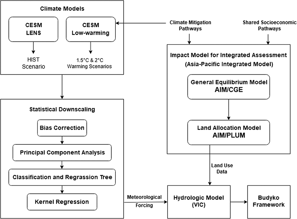
Figure 1. Methodological framework of the study.

Study Area

Our study is performed over the region of Ganga river basin, within the political boundary of India. The Ganga river basin is located within geographical coordinates of 73.5°E−89°E longitude and 22.5°N−31.5°N latitude. The basin consists of mountainous region at the northwest side, and the remaining area is plain encompassing northern and eastern India. The majority of the land in the Ganga basin plain is used for agriculture. The basin receives most of its rainfall over the summer monsoon season (June–September). Based on the Watershed Atlas of India, provided by the Central Ground Water Board (Ministry of Water Resources, Government of India), the basin is divided into 15 sub-basins, as shown in Figure 2.

FIGURE 2

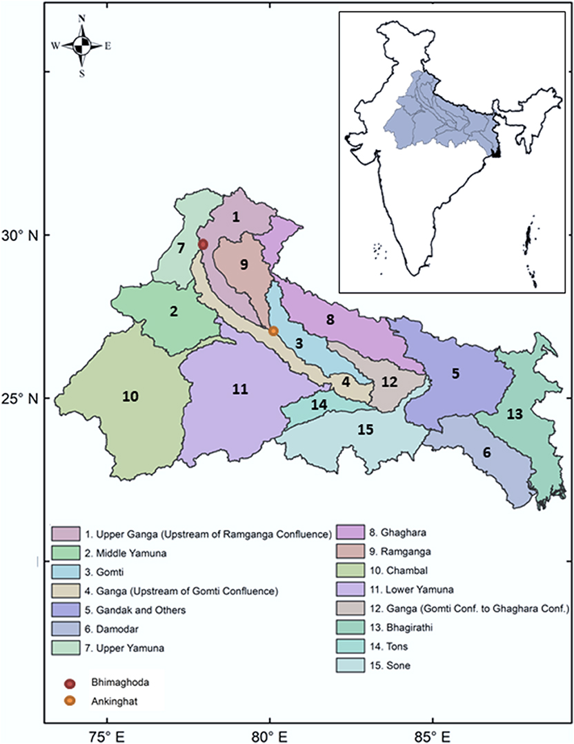
Figure 2. Study area: Ganga river basin divided into 15 sub-basins. Inlet is representing location of the basin within India. Location of streamflow measurement stations, Bhimaghoda and Ankinghat are marked with dots.

Scenario Matrix

In our study, 1.5 and 2°C warming scenarios are considered as climate change mitigation pathways, and SSP1, SSP2, SSP3, SSP4, and SSP5 are considered as socio-economic pathways. SSP1 (sustainability) represents low challenges for adaptation and mitigation, with low population growth, higher growth in per capita income and high environmental awareness. On the other hand SSP3 (regional rivalry) represents high challenges for adaptation and mitigation, due to increasing regional conflicts, less international trade, low income growth among the general population and low effort for environmental protection. SSP2 (middle of the road) represents medium challenges for both adaptation and mitigation, with modest population and economic growth with a slow pace of trade liberalization. SSP4 (inequality) represents high challenges in adaptation, due to increasing disparities in economic development among population, coupled with low challenges in mitigation due to technological advancement. Lastly SSP5 (fossil-fueled development) pushes for overall economic and social growth of general population by exploiting fossil fuel resources, depicting high challenges in mitigation with low challenges in adaptation. Apart from the aforementioned scenarios, a climate scenario with historical emissions (HIST) and a control socio-economic scenario with land use classes kept constant at year 2005 level (CTL) are also considered with the purpose of comparison. The overall scenario matrix for our study is presented in the Table 1. Each combined scenario in this matrix is named after the socio-economic scenario and warming scenario it belongs to. For example, the CTL_HIST scenario represents the control (CTL) socio-economic scenario and historical (HIST) emission scenario.

TABLE 1

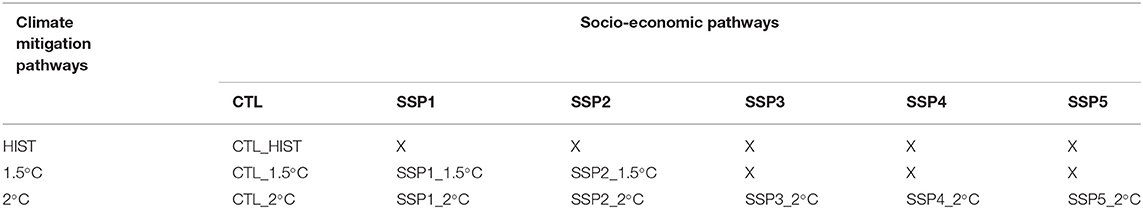
Table 1. Scenario matrix used in the study.

Climate Model Simulations

The climate model projections are obtained from CESM low-warming runs, performed using Community Earth System Model version 1 (CESM1) with Community Atmosphere Model version 5.2 (CAM5.2) and the Greenhouse gas (GHG) emission associated with 1.5 and 2°C warming scenarios, obtained from Minimal Complexity Earth Simulator (MiCES) (Sanderson et al., 2017). The historical climate scenario outcomes are obtained from CESM Large Ensemble (LENS) simulation (Kay et al., 2015), which are performed with the same CESM version and model parameters as the low-warming runs. Five ensembles of each simulation: Historical (HIST) (1951–2005), 1.5°C (2006–2100), and 2°C (2006–2100) were chosen for our study and bias correction and statistical downscaling methodologies are applied on each of them independently.

Statistical Downscaling

The outputs of CESM LENS and low-warming simulations are of coarse resolution (1° horizontal resolution) and not suitable for regional hydrological modeling. To use the model outcomes as meteorological forcing in hydrological model, they need to go through a bias correction and downscaling procedure. In this study, we have used a non-parametric regression-based multisite statistical downscaling method (Kannan and Ghosh, 2013; Salvi et al., 2013), where a statistical relationship is established between observed coarse resolution predictors (1° horizontal resolution) and fine resolution observed rainfall (0.25° horizontal resolution); and the derived relation is applied on the bias-corrected model-simulated predictors to obtain a better projection of future rainfall. In this study, for the development of statistical relationship between the predictors and rainfall, we have used daily reanalysis data from National Centers for Environmental Prediction/National Center for Atmospheric Research (NCEP/NCAR) (Kalnay et al., 1996), as proxy for observed predictors; and observed daily rainfall data from APHRODITE, Monsoon Asia (Yatagai et al., 2009), both for the period 1951–2005. The data from 1951 to 1980 is used for training the statistical model and the rest of the data is used for validation. The following climate variables have been used as predictors: air temperature, zonal and meridional wind at surface level; mean sea level pressure; air temperature, zonal and meridional wind, specific humidity at 850 hPa pressure level; and air temperature and geopotential height at 500 hPa pressure level. The downscaling methodology is performed for the entire landmass of India, by applying it separately for 7 meteorological homogeneous zones, suggested by India Meteorological Department (IMD) (Parthasarathy et al., 1996) and four seasons: June–September (JJAS), October–November (ON), December–February (DJF), and March–May (MAM). For each homogeneous zone, we have used a separate zone of predictors, as suggested by Salvi et al. (2013).

The downscaling methodology essentially involves four steps: bias correction, dimensionality reduction, rainfall state estimation, and rainfall value estimation through regression. First, we have bilinearly interpolated the model-simulated predictors to the same grids as reanalysis predictors and used a quantile mapping method proposed by Li et al. (2010), for correcting the bias in the model data. A distribution is fitted to all the grids separately for both reanalysis and model data. We have fitted Normal distribution for wind and specific humidity and Gamma distribution for rest of the predictors. Then, for the historical period (1951–2005), the Cumulative Distribution Function (CDF) of the reanalysis and the model-simulated data are compared and the biased model data at each grid and time step is replaced by the reanalysis data with same CDF. For future (2006–2100), additionally, the shift between model-simulated historical and future data with same CDF is added to the replacement value, to account for the climate change. Apart from the predictors used in the statistical downscaling of precipitation, we have also bias-corrected daily minimum and maximum temperature, which are later used as meteorological forcing in the hydrological model. Next, in order to get rid of the multidimensionality and multicollinearity of the predictors, we have used principal component analysis (PCA) on the reanalysis predictors. We have sorted the principal components in the descending order based on their explained variance and taken the first few of them till the sum of explained variance reached 80%. The same coefficients were used to transform the model simulated predictors also. We have classified the observed rainfall into 3 states using unsupervised K-means clustering and apply Classification and Regression Tree (CART) to establish a relationship between reanalysis predictor PCs and observed rainfall states. We have then applied the derived relation on Model predictor PCs to estimate the rainfall state. For each rainfall state, we have applied Kernel Regression on the predictor PCs to obtain the projected daily rainfall amounts. We have used the Nadaraya-Watson estimator for kernel density estimates (Nadaraya, 1964) and asymptotic mean integrated square error (AMISE) criteria for bandwidth selection (Wand and Jones, 1995; Scott, 2015). The final resolution of the downscaled rainfall is same as that of the observed rainfall, which is 0.25° in our case. After downscaling is performed, rainfall and other meteorlogical variables for the grids belonging to Ganga basin region are extracted to be used as an input to the hydrological model.

The performance of the downscaling model is presented in Figure 3. The difference between mean observed and projected JJAS rainfall for validation period (1981–2005) doesn't exceed 3 mm for majority (98%) of the grids. Standard deviation is underestimated in the projected rainfall. For more than 96% of the grids, difference between standard deviation of projected and observed JJAS rainfall is within 6 mm/day. Overall, we find the performance of the model satisfactory. More discussion on the performance of the model can be found on Salvi et al. (2013).

FIGURE 3

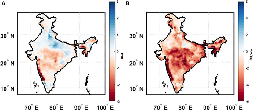
Figure 3. Performance of statistical downscaling model. (A) Difference between mean projected JJAS rainfall and observed JJAS rainfall for validation period (1981–2005) (B) Difference between projected standard deviation of JJAS rainfall and observed standard deviation of JJAS rainfall for validation period (1981–2005).

Land Allocation Model

The gridded land use projections are obtained from the impact model Asia-pacific Integrated Model (AIM). The computable general equilibrium (AIM/CGE) component is a recursive-dynamic general equilibrium model, which takes population, gross domestic product (GDP), consumption, technological progress, pollution level etc. associated with socio-economic pathways into account and provides regionally aggregated emission, energy, and land use information for each scenario in SSP-RCP scenario matrix (Fujimori et al., 2017). This aggregated land use projections are then regionally disaggregated into 0.5° × 0.5° gridded land use data by the land allocation model AIM/PLUM. Land allocations are performed to maximize the economic efficiency for a given biophysical land productivity (Hasegawa et al., 2017). The outcomes of AIM/PLUM are available globally for the year 2005 and then every 10 years from 2010 onwards, which we have extracted for our study region. It should be noted that the outcomes of this model are available for emission based RCPs, not temperature based climate scenarios we are using in our study. However, RCP1.9 and RCP3.4 have been used among climate mitigation pathways for AIM; even though they are not part of the originally proposed pathways (Van Vuuren et al., 2011), today they are widely used as analogous to 1.5 and 2°C warming scenarios (Fujimori et al., 2018).

Hydrologic Simulation

The projected meteorological data and land use data are forced grid-wise into a semi-distributed mesoscale hydrological model (VIC), which balances water and surface energy budgets. The key characters of the VIC model includes representation of multiple land cover types on a single grid, spatial variability of soil moisture capacity, multiple soil layers, and interactions between them, non-linear base flow and clumped vegetation formulation with time-varying spacing between plants (Bohn and Vivoni, 2016). A list of datasets used as an input to the hydrological model is presented in Table 2. The elevation map for VIC is acquired from U.S. Geological Survey (USGS) HYDRO1K dataset (Raje et al., 2014). Vegetation parameters, such as leaf area index, are collected from Global Land Data Assimilation Systems (GLDAS) dataset (Rodell et al., 2004). Soil data is extracted from a global database from Food and Agriculture Organization (FAO) at 0.5° resolution. Certain soil parameters, such as soil depth, are obtained by calibrating the model at two stations, Ankinghat and Bhimaghoda. The observed streamflow for these two stations are collected from Central Water Commission (CWC), India at monthly scale (Chawla and Mujumdar, 2015; Joseph et al., 2018). After calibration, the comparison of observed and VIC simulated streamflow is presented in Figures 4A,B. We have also calculated Nash-Sutcliffe efficiency (NSE) of the model in each station. The model simulated streamflow matches the observed flow reasonably well at Bhimaghoda station (NSE = 0.75), but overestimated at the Ankinghat station (NSE = 0.09). It should be noted that the flow is highly regulated at downstream, which may have contributed to the relatively poor performance of the model at Ankinghat station. We have tried to minimize the impact of human water management in the streamflow data, by incorporating data from water diversion structures and canals. We have validated our model against an observed evapotranspiration data collected from Moderate Resolution Imaging Spectroradiometer (MODIS) MOD16 Global Terrestrial Evapotranspiration Data Set and a satellite based soil moisture data from European Space Agency Climate Change Initiative, for the time period 2000–2009, results of which are presented in Figures 4C,D, respectively. Overall the simulated evapotranspiration and soil moisture show high positive correlation for majority of the grids in our study area.

TABLE 2

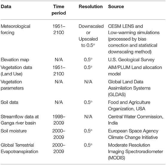
Table 2. Datasets used in hydrological modeling or validation.

FIGURE 4

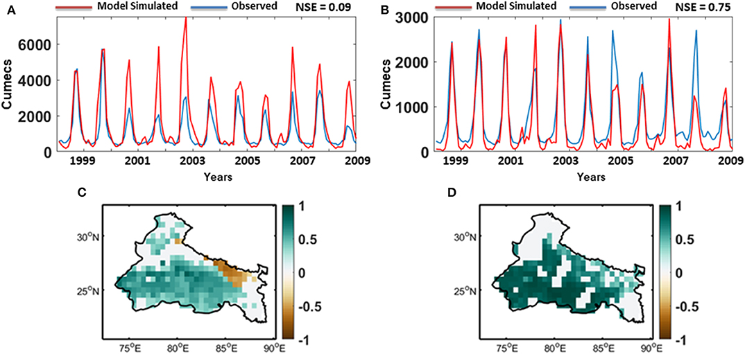
Figure 4. Calibration and Validation of hydrologic model VIC. (A) Time series of monthly observed (blue) and model simulated (red) streamflow at Ankinghat station. (B) Time series of monthly observed (blue) and model simulated (red) streamflow at Bhimaghoda station. (C) Correlation of observed and model simulated evapotranspiration during JJAS season at 95% significance level. (D) Correlation of observed and model simulated soil moisture during JJAS season at 95% significance level.

Budyko Framework

Budyko (1974) proposed a deterministic non-parametric framework to model the long-term water budget constrained by atmospheric water supply and water demand limit. According to this framework, the evaporative fraction (ratio of evapotranspiration to precipitation) can be expressed as a function of aridity index (ratio of potential evapotranspiration to precipitation). However, the relationship between evaporative fraction and aridity changes among catchments and to account for that various functional forms of Budyko equation has been proposed in scientific literature (Fu, 1981; Choudhury, 1999). In these Budyko equations, basin characteristics parameter is introduced, which, by definition, explains the combined effect of all factors other than aridity on the terrestrial water balance. In this study we use the following functional form of the Budyko equation, known as the Mezentsev equation.

\begin{array}{l} \frac{E}{P} = {(1 + {(\frac{E_{0}}{P})}^{- n})}^{\frac{- 1}{n}} & (1) \end{array}

Where P is the precipitation, E is the evapotranspiration, E₀ is potential evpotranspiration and n is the basin characteristics parameter.

One assumption of Budyko framework is that the long term change in mean water storage is negligible and the whole incoming precipitation either evaporates or contributes to runoff. However, our study focuses on the long term mean of seasonal (JJAS) rainfall, this assumption does not hold true. In order to apply the Budyko framework to long-term mean of seasonal rainfall, we have introduced the change in storage (ΔS) in the equation.

\begin{array}{l} \frac{E}{P - Δ S} = {(1 + {(\frac{E_{0}}{P - Δ S})}^{- n})}^{\frac{- 1}{n}} & (2) \end{array}

In this study, we apply the Equation 2 on the hydrological outcomes obtained from VIC for each of the 15 sub-basins and each scenario to estimate the basin characteristics parameter, in order to understand the relative impacts of climate and land use changes on the basin characteristics.

Results

In Figure 5 we have presented the projected climate change at the Ganga river basin in terms of mean precipitation during monsoon (JJAS). The changes are calculated between last 25 years of each century (1976–2000 for HIST and 2076–2100 for future scenarios), which remains true throughout this study, unless otherwise mentioned. We have found an east–west asymmetry in the projected rainfall changes. The eastern part of the basin shows an increase in rainfall in the twenty-first century, where the western part, which is part of the core monsoon zone, is projected to have a declining trend in the warming scenario. The extent of this asymmetry is higher in the 2°C warming scenario comparatively. As a similar spatial pattern has been found in the present day observed rainfall trend (Das et al., 2014), this asymmetry can be considered a characteristic climatic response of the Ganga basin region to global warming.

FIGURE 5

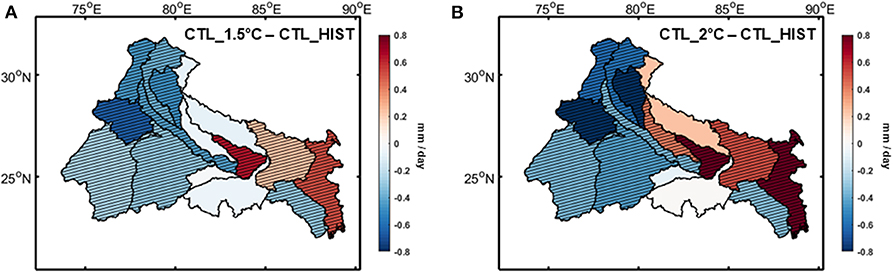
Figure 5. Changes in downscaled precipitation from HIST to 1.5°C (A) and from HIST to 2°C (B) for CTL scenario over Ganga river basin for JJAS season. Hatched regions denote areas with statistically significant changes.

In Figure 6 we have shown the time evolution of various land use classes throughout the twenty-first century, as projected by AIM/PLUM model for the Ganga basin region. The outputs of the land allocation model are provided at 0.5° × 0.5° grids, which are aggregated to prepare the projection for the whole basin. Figure 6A shows the changes in cropland, which covers the majority of the lands in our study area. In every scenario the cropland area increases during the first few decades and then starts declining throughout the century. The SSP3_2°C scenario, which is the least sustainable among all, doesn't feature this decline in cropland area and roughly maintain its peak throughout the century. Figure 6B depicts the projected area of unmanaged forests, which shows a decline at the beginning, but gets reversed into an increasing trend for some scenarios. For the scenarios associated with low challenges for mitigation (i.e., SSP1 and SSP4) we find this increasing trend in forest land in the latter part of the century; however the others scenarios continue to show decline throughout the century. In Figure 6C we have shown the projected changes associated with pasture lands, which are comparatively smaller than the previous two land classes. Overall, pasture land area is projected to increase after an initial decrease. In most cases the direction of changes are closely tied with and opposite to the changes in cropland for that specific scenario.

FIGURE 6

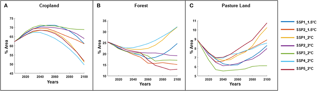
Figure 6. Time evolution of percentage area of (A) cropland, (B) forest, and (C) pasture land at Ganga river basin, for each combination of RCP-SSP scenario over twenty-first century, as projected by AIM/PLUM model.

In Figures 7–10, we have compared the relative impacts of projected climate and land use changes on the hydrometeorological variables at Ganga river basin, as captured by the VIC simulations. Even though the impacts of these changes are not perfectly linearly additive, we can roughly estimate them by subtracting the outcomes of various VIC experiments from each other. For example, subtracting the outcomes of CTL_HIST experiment from CTL_1.5°C experiment will give us an estimate of the impact of 1.5°C warming scenario. On the other hand, the impacts of land use change associated with SSP1_1.5°C scenario can be estimated by subtracting the outcomes of CTL_1.5°C experiment from that of SSP1_1.5°C experiment. The statistical significance of these differences are estimated using t-test with a 95% significance level and the sub-basins showing significant differences are highlighted in the figures. We have found a few notable patterns consistent across the hydrologic variables. In Figures 7A,D, 8A,D, 9A,D, 10A,D we have shown the impacts of 1.5 and 2°C warming on evapotranspiration, total runoff (surface runoff and baseflow), potential evapotranspiration, and aridity index at the Ganga river basin, respectively. As evapotranspiration and runoff are correlated with precipitation, the spatial patterns of their changes closely resemble the projected precipitation trend. The east-west asymmetries are still present here. On the other hand potential evapotranspiration is correlated with temperature and projected to increase almost uniformly throughout the basin. In case of aridity of the basin, even though the asymmetry in changes can still be noticed, majority of the sub-basins show an increase in the warming scenario, implying increased water stress as a result of global warming. Figures 7B,C, 8B,C, 9B,C, 10B,C show the impact of land use changes associated with SSP1-2 and 1.5°C warming and Figures 7E–I, 8E–I, 9E–I, 10E–I represent the same for SSP1-5 and 2°C warming for evapotranspiration, total runoff, potential evapotranspiration, and aridity index, respectively. We have found that hardly any changes associated with land use are visible in the figures, which suggests that the impacts of projected land use changes are negligible compared to its climate change counterpart. Neither of these hydrologic variable changes shows any significant contribution from the projected land use changes for most of the basins. However, there are a few exceptions in some of the sub-basins. For example, the Bhagirathi sub-basin gets more arid in few SSP scenarios, but doesn't show any significant change when only climate change is considered. These exceptions are a result of potential evapotranspiration increasing proportionately with precipitation due to climate change, but not being impacted significantly because of land use change.

FIGURE 7

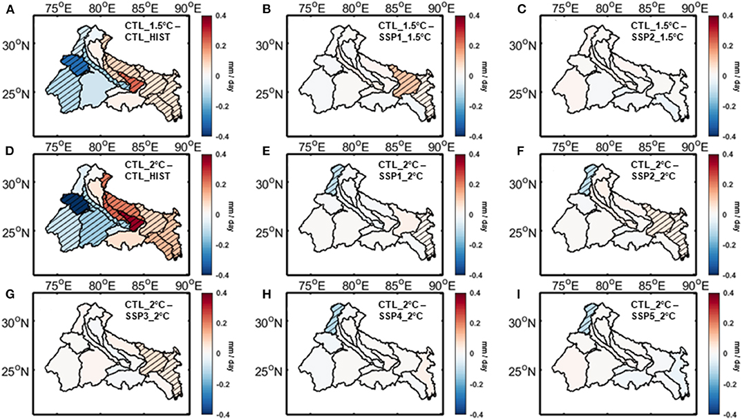
Figure 7. Changes in VIC simulated evapotranspiration associate with climate change for (A) 1.5°C warming, (D) 2°C warming and land use change for (B) SSP1_1.5°C scenario, (C) SSP2_1.5°C scenario, (E) SSP1_2°C scenario, (F) SSP2_2°C scenario, (G) SSP3_2°C scenario, (H) SSP4_2°C scenario, (I) SSP5_2°C scenario over Ganga river basin. Hatched regions denote areas with statistically significant changes.

FIGURE 8

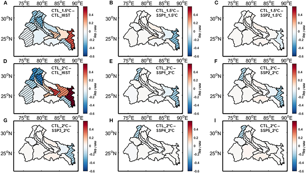
Figure 8. Changes in VIC simulated total runoff associate with climate change for (A) 1.5°C warming, (D) 2°C warming and land use change for (B) SSP1_1.5°C scenario, (C) SSP2_1.5°C scenario, (E) SSP1_2°C scenario, (F) SSP2_2°C scenario, (G) SSP3_2°C scenario, (H) SSP4_2°C scenario, (I) SSP5_2°C scenario over Ganga river basin. Hatched regions denote areas with statistically significant changes.

FIGURE 9

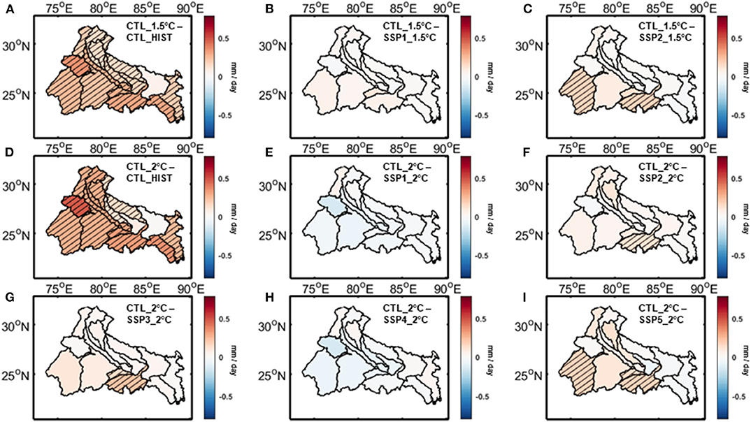
Figure 9. Changes in VIC simulated potential evapotranspiration associate with climate change for (A) 1.5°C warming, (D) 2°C warming and land use change for (B) SSP1_1.5°C scenario, (C) SSP2_1.5°C scenario, (E) SSP1_2°C scenario, (F) SSP2_2°C scenario, (G) SSP3_2°C scenario, (H) SSP4_2°C scenario, (I) SSP5_2°C scenario over Ganga river basin. Hatched regions denote areas with statistically significant changes.

FIGURE 10

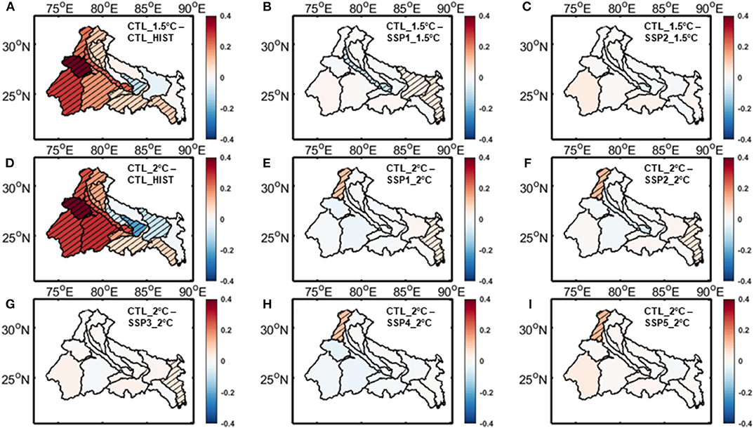
Figure 10. Changes in VIC simulated aridity index associate with climate change for (A) 1.5°C warming, (D) 2°C warming and land use change for (B) SSP1_1.5°C scenario, (C) SSP2_1.5°C scenario, (E) SSP1_2°C scenario, (F) SSP2_2°C scenario, (G) SSP3_2°C scenario, (H) SSP4_2°C scenario, (I) SSP5_2°C scenario over Ganga river basin. Hatched regions denote areas with statistically significant changes.

From the VIC simulated hydrologic variables, we have calculated the value of basin characteristics parameter (n) for each sub-basin using Budyko framework (Equation 2). The result is presented in Table 3. We have found two notable patterns in this data. Firstly, the basin characteristics is influenced by climate change. As the warming goes higher from HIST to 1.5–2°C, many sub-basins show a consistent increase or decrease in the projected basin characteristics parameter. Secondly, the impact of projected land use changes is not as prominent. For the majority of the sub-basins there is hardly any difference between SSP scenarios and their CTL counterpart for the same level of warming. However, there are a few exceptions to this pattern. In certain scenarios, the land use changes have been found to have some impact in Bhagirathi, Tons, Sone, Damodar, and Gandak and others sub-basins, although not as high as the climate impact in most cases. The reasons behind these exceptional cases are unclear, and require further examinations to be uncovered. Given that all of these sub-basins are located at the east side of the basin, it can be speculated to be related to the east-west asymmetry of climate change response.

TABLE 3

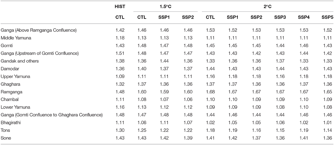
Table 3. Calculated basin characteristics parameter for all sub-basins and scenarios.

Discussions

There are multiple sources of uncertainty present in our modeling framework. Our choices of climate change mitigation pathways as well as parameterizations in climate model simulations and their internal climate variability (Knutti and Sedláček, 2013) are major sources of uncertainties, although it is partly mitigated by considering multi-ensemble mean of climate model outcomes. Our choices of socioeconomic pathways, the impact model (AIM) and the statistical downscaling methodology, all contribute substantially to the uncertainty of the climate and land use projections. The assumption of linear responses of land use and climate change to the hydrologic variables imposes some uncertainties as well. The parameter uncertainty in the hydrologic model is also responsible for a significant portion of the overall uncertainties (Chawla and Mujumdar, 2018), although they are relatively lower than the uncertainties resulting from climate models and downscaling methods (Joseph et al., 2018). However, we believe that the presence of these uncertainties in the projections do not affect the key findings of our study. The hydrologic changes associated with climate change are significantly higher than that of land use change, close to one magnitude of order in many cases. This pattern is also consistent across hydrologic variables, scenarios and sub-basins. Our finding is consistent with Chawla and Mujumdar (2015)'s analysis on Upper Ganga basin for historical climate and land use changes. Analyzing our data in the Budyko framework also shows that the climatic variables have a significant impact on the basin characteristics, while vegetation has lesser impact, which is contrary to the traditional assumption. This finding is consistent with Padrón et al. (2017) and Abatzoglou and Ficklin (2017)'s global analyses with observed datasets in historical time period. The methodology used in our study is generic and can be applied to other river basins as well. However, the conclusion of this analysis may vary depending on the climate and land use of the basin. Worldwide, there have been multiple attempts to distinguish between climate and land use change impacts on basin-scale hydrology, even though majority of the studies are for historical period and very few studies consider projections for future scenarios. The conclusions drawn in these studies are mixed; while some studies have found significant contributions from land use changes (Schilling et al., 2008; Wang and Hejazi, 2011), others have found it to be negligible (Gupta et al., 2015).

Concluding Remarks

In this study we have explored the impacts of projected climate change as well as land use changes on the terrestrial water balance at river basin scale. We have found that a major part of the Ganga river basin is projected to become significantly more arid in the warming scenarios. However, the projected land use changes hardly contributes to or counteracts climate change impacts. In contrast with the traditional assumption, climatic variables are found to have significantly more impacts on basin characteristics compared to land use and vegetation. Overall, our results show that, in terms of hydrologic impact assessment, climate change mitigation pathways are the dominant factor and the land use changes associated with socio-economic pathways contribute little to alleviate the impacts of climate change.

Data Availability Statement

The datasets generated for this study are available on request to the corresponding author.

Author Contributions

SG designed the problem and reviewed the manuscript. AS performed the required computation, wrote the manuscript, and prepared the figures. SG and AS analyzed the results.

Funding

The CESM LENS and Low warming simulation data are collected from Earth System Grid (https://www.earthsystemgrid.org). The observed precipitation data is collected from APHRODITE (www.chikyu.ac.jp/precip/english/products.html) and NCEP/NCAR Reanalysis data are collected from Earth System Research Laboratory (https://www.esrl.noaa.gov/psd/data/gridded/data.ncep.reanalysis.html). The elevation data is acquired from U.S. Geological Survey; Gridded land use projection data is acquired from AIM (http://www-iam.nies.go.jp/aim/data_tools/aimssp/aimssp.html); soil data is collected from Food and Agriculture Organization, USA; observed streamflow data is acquired from Central Water Commission, India; satellite based soil moisture data is collected from European Space Agency Climate Change Initiative; observed evapotranspiration data is acquired from MODIS MOD16 Global Terrestrial Evapotranspiration Data Set.

Conflict of Interest

The authors declare that the research was conducted in the absence of any commercial or financial relationships that could be construed as a potential conflict of interest.

Acknowledgments

The authors acknowledge the financial support from Ministry of Earth Sciences, Government of India through MoES-NERC Newton Bhaba funding (MoES/NERC/IA-SWR/ P2/09/2016-PC-II) and from Department of Science and Technology (SPLICE—Climate Change Programme), Government of India, Project reference number DST/CCP/CoE/140/2018, Grant Number: 00000000000010013072 (UC ID: 18192442).

References

Abatzoglou, J. T., and Ficklin, D. L. (2017). Climatic and physiographic controls of spatial variability in surface water balance over the contiguous United States using the budyko relationship. Water Resour. Res. 53, 7630–7643. doi: 10.1002/2017WR020843