 Ganesh R. Ghimire
 Navid Jadidoleslam
 Witold F. Krajewski
 Anastasios A. Tsonis2,3
- 1IIHR-Hydroscience and Engineering, The University of Iowa, Iowa City, IA, United States
- 2Department of Mathematical Sciences, University of Wisconsin-Milwaukee, Milwaukee, WI, United States
- 3Hydrologic Research Center, San Diego, CA, United States
Streamflow is a dynamical process that integrates water movement in space and time within basin boundaries. The authors characterize the dynamics associated with streamflow time-series data from 64 U.S. Geological Survey (USGS) unregulated stream-gauge stations in the state of Iowa. They employ a novel approach called visibility graph (VG) that uses the concept of mapping time series into complex networks to investigate the time evolutionary behavior of dynamical systems. The authors focus on a simple variant of the VG algorithm called horizontal visibility graph (HVG). The tracking of dynamics, and consequently the predictability of streamflow processes is carried out by extracting two key pieces of information called characteristic exponent, λ, of degree distribution and global clustering coefficient, GC, pertaining to the HVG-derived network. The authors use these two measures to identify whether streamflow has its origin in random or chaotic processes. They show that the characterization of streamflow dynamics is sensitive to data attributes. Through a systematic and comprehensive analysis, the authors illustrate that streamflow dynamics characterization is sensitive to the normalization and the time scale of streamflow time series. At a daily scale, streamflow at all stations used in the analysis reveals randomness with strong spatial scale (basin size) dependence. This has implications for predictability of streamflow and floods. The authors demonstrate that dynamics transition through potentially chaotic to randomly correlated processes as the averaging time scale increases. Finally, the temporal trends of λ and GC are statistically significant at about 40% of the total number of stations analyzed. Attributing these trends to factors such as changing climate or land use requires further research.
Introduction
Transport of water in streams and rivers is a main component of the hydrologic cycle characterized by streamflow fluctuation over time. Causes of streamflow fluctuations include intense rainfall events leading to high flows and floods; longer inter-storm periods followed by low flows and droughts; and snowmelt in higher latitudes after cessation of cold season. Improving our ability to predict streamflow over short and long-time horizons requires a better understanding of streamflow variability and the underlying dynamics. In this study, the authors treat streamflow time series as an output of a non-linear dynamical system and map them into complex networks using an algorithm based on a visibility graph (VG) concept (e.g., Lacasa et al., 2008, 2012; Lacasa and Toral, 2010; Stephen et al., 2015; Braga et al., 2016).
Streamflow time series have been studied using many different approaches, including Fourier transforms (e.g., Lundquist and Cayan, 2002), wavelet transforms (e.g., Smith et al., 1998; Coulibaly and Burn, 2004), chaos theory (e.g., Porporato and Ridolfi, 1997; Bordignon and Lisi, 2000), and stochastic modeling (e.g., Livina et al., 2003; Prairie et al., 2006; Wang, 2006). Most of these studies were motivated by the needs of streamflow forecasting, however, addressing a broader concept of predictability (e.g., Kumar, 2011) raises questions about the origins of the underlying processes (e.g., Lacasa and Toral, 2010).
The problem of mathematical and numerical modeling to understand the predictability of streamflow requires distinguishing whether the underlying dynamics are deterministic or stochastic. In this direction, limited efforts have been documented in the hydrologic literature. Porporato and Ridolfi (1997) and Bordignon and Lisi (2000) checked for the evidence of chaotic behavior considering measures such as phase-portrait of the attractor, largest Lyapunov exponent, and correlation dimension. They demonstrated that the presence of a low-dimensional chaotic (deterministic) component could not be excluded. Bordignon and Lisi (2000) further verified the presence of chaotic behavior using the deterministic vs. stochastic (DVS) algorithm proposed by Casdagli and Weigend (1993). Their study showed that non-linear river flow modeling enhances predictability. Pasternack (1999) investigated the presence of low-dimensional chaos in hydrological systems using correlation integral analysis (CIA) (see Grassberger and Procaccia, 1983) and demonstrated that daily streamflow time series for relatively pristine rivers do not show chaotic behavior. Overall, there has not been a clear consensus in the literature regarding the identification of chaotic behavior in streamflow time series (see e.g., Pasternack, 1999; Koutsoyiannis, 2006).
This study is focused on networks. A network is defined by a set of nodes and their links, where any pair of nodes is connected according to some rule. The nodes in a network can be anything. For example, in a network of actors, the nodes are actors that are connected to other actors if they have appeared together in a movie. In a network of species, the nodes are species that are connected to other species they interact with. In a network of scientists, the nodes are scientists that are connected to other scientists if they have collaborated. In the grand network of humans each node is an individual who is connected to people he or she knows. When networks were introduced to the climate community (Tsonis and Roebber, 2004; Tsonis et al., 2006), nodes were grid points in a field (e.g., 500 hPa field). Links in that network were defined according to a threshold in the correlation coefficient between the time series of any given pair of grid points.
There are several types of networks. On the two extremes are regular and random networks. Regular networks have a fixed number of nodes, each node having the same number of links connecting it in a specific way to a number of neighboring nodes. In random networks, the nodes are connected at random. Other networks have been discovered, such as small-world networks (a combination of regular and random networks) and scale-free networks (characterized by a few nodes having many connections and many nodes having few connections). The topology of the network can reveal important and novel features of the system it represents (Strogatz, 2001; Albert and Barabási, 2002; Costa et al., 2007).
Since the discovery of small-world networks by Watts and Strogatz (1998), the study of networks has developed with new approaches to constructing networks and studying their topology. One of the latest methods is the one we will employ here. This particular method is attractive because it provides a criterion that distinguishes between chaotic and stochastic processes. In this method, any time series can be mapped into a complex network (graph) (e.g., Lacasa et al., 2008, 2012; Luque et al., 2009; Lacasa and Toral, 2010; Stephen et al., 2015; Braga et al., 2016). Analysis of the properties of the network can reveal the nature of the dynamics that created the time-series data.
Lacasa and Toral (2010) employed HVG to distinguish between random and chaotic processes underlying a time series. They showed that a time series maps to a network where the number of connections with other nodes (called degree distribution) has an exponential distribution. Lacasa and Toral (2010) and Braga et al. (2016) have shown analytically that, irrespective of the underlying distributions, the value of the characteristic exponent parameter of degree distribution serves as the exact frontier between chaotic and stochastic processes. Another characteristic of the network is the clustering coefficient, which measures the likelihood of nodes to form clusters of tightly knit groups with a relatively high density of ties (see e.g., Watts and Strogatz, 1998; Newman, 2003; Tsonis et al., 2006; Braga et al., 2016). A specific form of clustering coefficient that deals with the clustering nature of the entire network rather than its local behavior is called the global clustering coefficient, GC. GC is designed to give an overall indication of the clustering in the network, which is directly related to how stable a network is. As GC approaches the value of 1, the network becomes fully connected (every node is connected to every other node); as it approaches 0, the network becomes completely disconnected. In the case of a network derived from a time series, a GC = 1 will indicate that every point “sees” every other point, therefore the process is perfectly linear.
Gonçalves et al. (2016) explored HVG in new ways using information theory. They showed that alternatives to degree distributions such as distance distribution and weight distribution can help extract efficient information, especially for shorter time series. Recently, Braga et al. (2016) used HVG to analyze river flow fluctuations at a daily time scale using 141 stream gauges in Brazil. They demonstrated the presence of correlated stochastic structure in the streamflow dynamics through degree distribution and GC. Further, Lange et al. (2018) investigated the sensitivity of the HVG methodology to streamflow time series pre-processing properties such as time series length, presence of ties in the data, and effects of seasonality, using around 150 time series from managed rivers in Brazil at a daily time scale. They showed that data pre-processing can result in contradictory results and thus should be used with caution. Serinaldi and Kilsby (2016) used a directed HVG, in which each node is connected to past nodes or to future nodes (represented by arrows) to explore time irreversibility (or temporal asymmetry, see Lacasa et al., 2012), a signature of the non-linearity of streamflow through analysis of degree distributions. In their comprehensive study, they used 699 unregulated daily time scale streamflow time series across the conterminous United States (CONUS) to show that degree distributions have systematic sub-exponential behaviors of different strengths and quantified the results through the information theory measures. Their findings show that streamflow dynamics are more complex than simple stochastic linear dynamics, and irreversibility is a key feature.
In this work, we study unregulated streamflow time series at United States Geological Survey (USGS) stream gauge stations in the U.S. state of Iowa using networks derived from simple undirected HVG, in which each node is connected to past and future nodes (represented by lines). Our objective is not only to explore the predictability of streamflow dynamics in terms of processes generating them, but also to gain insights regarding questions not addressed by previous works. Specifically, we address the following questions: (1) What processes underlie streamflow dynamics? (2) How does time resolution of streamflow time-series data, as well as a normalization procedure, impact inference from HVG-based networks? (3) Does the complex network description of the streamflow process demonstrate spatial (basin) scale dependence? (4) Do the characteristics describing this process show temporal evolution?
This paper is organized as follows. In the methods section, we present the study area and streamflow time-series data and provide HVG application strategy across time scales. In the results and discussion section, we seek answers to the above questions based on results from our analysis. Finally, we draw conclusions from this work and outline avenues for further research on visibility-based network analysis of streamflow dynamics.
Data and Methods
To construct the network, consider two arbitrary data points of a time series [ta, xa] and [tc, xc] with any other data point [tb, xb] such that ta < tb < tc. The VG algorithm defines these time steps ta, tb, and tc as nodes of the network such that xa and xc are visible to each other and are connected (see Luque et al., 2009) if,
Such networks (graphs) have the ability to reveal many salient characteristics of the time series. Regardless of the type of time series used, the constructed network is, by definition, connected and invariant to affine transformations of the time series. Hence, the constructed network from a time series maintains its inherent properties.
A simple variant to VG is the horizontal visibility graph (HVG). Mathematically, let [xi, i = 1, 2,…, N] be a time series of N data, where i represents nodes. Two nodes i and j are connected if,
Graphically, two nodes i and j are connected if one can draw a horizontal line in the time series joining xi and xj, which does not intersect any intermediate data. A key feature of HVG graphs is that the nearest neighbors are visible to each other. Note that rescaling of horizontal and vertical axes and horizontal and vertical translations do not affect the resultant network. In Figure 1, we illustrate the concept of transforming time series to a network using HVG. We use this approach to generate the network from a streamflow time series to explore its underlying dynamics.
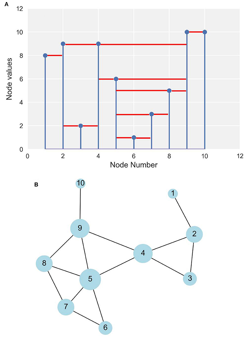
Figure 1. Schematic illustration of horizontal visibility graph (HVG) approach. (A) Indices of nodes with corresponding values. The solid red lines show whether corresponding nodes are horizontally visible to each other. For example, in node 4 we can draw a horizontal straight line between node 4 and node 2 that does not intersect the height of node 3. Thus, node 4 is connected to node 2. Similarly, node 4 is connected to nodes 3, 5, and 9, but not, for example, node 6, since there is no way we can draw a horizontal line without crossing the height of node 5. (B) The complete network.
The midwestern state of Iowa contains many streams and rivers draining to the Mississippi River in the east and the Missouri River in the west. About 65% of the state drains to the Mississippi River, while about 35% of the state drains to the Missouri River (e.g., Larimer, 1957; Ghimire et al., 2018). Most of the land use in the state is agricultural. The northeastern part of the state is characterized by deeply carved terrain, narrow valleys, and relatively higher stream slopes, while low reliefs with relatively milder stream slope make up the rest of the state (e.g., Ghimire et al., 2018). Most significant streamflow events (e.g., floods) occur in the spring and early summer. However, significant events occasionally occur at other times of the year. Snowmelt has rather minor direct effect but can influence flooding by keeping soils saturated into late spring.
At present, around 140 USGS streamflow gauges monitor these streams and rivers, providing data for this study. Figure 2 shows the spatial distribution of the USGS stations across Iowa. We considered unregulated USGS daily streamflow records with record length of at least 50 years. Sixty-four stations meet this criterion, as depicted by dark green dots in Figure 2. The longest record is 115 years. Since higher resolution data (i.e., sampled at 15-minute intervals) are available only since 2002, we used data from 2002 through 2018 for analysis at instantaneous and hourly scales. We used 15-min streamflow time series first and averaged the data to generate subsequent hourly (using four nodes) and daily (using 96 nodes) scale streamflow time series.
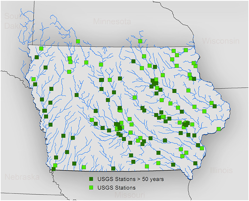
Figure 2. Spatial distribution of USGS stations (both light and dark green squares) across Iowa. The dark green squares represent USGS stations with at least 50 years of streamflow records.
The USGS stream gauges measure discharge from drainage areas that range from about 7 km2 to 37,000 km2. Figure 3A illustrates the distribution of basin scales, and Figure 3B illustrates the distribution of daily streamflow records length of USGS stations, respectively. The wide range of monitored basin sizes enables us to capture the spatial scale dependence of HVG-derived information measures.
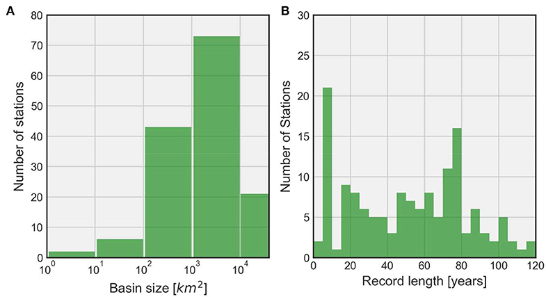
Figure 3. Histogram of USGS basin characteristics. (A) Distribution of basin scales across Iowa; (B) distribution of streamflow record lengths in terms of number of stations.
We constructed networks representing every year of the historical streamflow records for the USGS stations described above. For each year, there are 365 nodes represented by the index I = 1,2,…,365 such that N = 365 at a daily time scale. To avoid major seasonal trends between years, we standardized (normalized) the time series using the mean and standard deviation of flows for each day of the year (e.g., Braga et al., 2016; Serinaldi and Kilsby, 2016; Lange et al., 2018), a typical procedure for such hydrologic analyses. We discuss later the impact of this transformation on inferences derived from the networks. Let Xt(i) represent the flow in the year “t” on the day “i.” Likewise, let xt(i) be the normalized flow for the year “t” on the day “i.” Then, we define the normalization of time series through Equations (1)–(3).
where
and
represent the mean and standard deviation of the flow respectively on the day “i” obtained from the distribution over the years of historical records at the given station [n∈(50, 115)]. As an illustration, we present in Figure 4 the envelope of the entire record of daily streamflow together with its mean and median (see Figures 4A,C) as well as the corresponding envelope of the normalized flows (see Figures 4B,D) for a large basin (16,800 km2) of the Cedar River at Cedar Rapids and a small basin (70 km2) of Rapid Creek near Iowa City, respectively. It is apparent that the seasonality of flows clearly visible in the original series is much reduced in the normalized data.
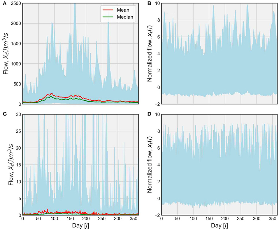
Figure 4. Streamflow time series normalization for two basins. (A) Shaded envelope representing an ensemble of entire raw streamflow records, Xt(i), at a daily scale for the Cedar River at Cedar Rapids (16,800 km2). This envelope shows the variability of streamflow, σ(i), while the red and green lines represent mean, μ(i), and median of flows, respectively. (B) Shaded envelope representing an ensemble of normalized streamflows, xt(i), corresponding to (A). (C) Raw streamflow time series at Rapid Creek near Iowa City (70 km2) with same description as (A). (D) Normalized streamflow time series corresponding to (C).
Next, we mapped the time series for every year to a complex network using HVG. An illustration of the network associated with two streamflow time series is presented in Figure 5. Figure 5A corresponds to the network associated with normalized time series at the Cedar River at Cedar Rapids (16,800 km2), while Figure 5B shows the network of streamflow obtained from the same daily data but shuffled randomly over time. The color code represents the month of a year associated with each node, with their size representing the number of connections they make with their neighbors. Clearly, larger nodes of the HVG-derived network are associated with the major events. As Figure 5A shows, the nodes related to consecutive months (neighbors in proximity) are connected to each other, implying the information transfer during streamflow generation process in the form of antecedent soil moisture, base flow, and other factors.
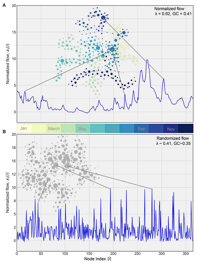
Figure 5. HVG-derived network for the Cedar River at Cedar Rapids for 2016. (A) Network associated with normalized flow (corresponds to Figure 4). Each color represents the corresponding month of a year where the size of each node corresponds to the number of connections with its neighbors. (B) Network for randomly shuffled streamflow from (A). In the normalized data λ > 0.41 indicates the presence of a stochastic process. Both λ and GC are lower in the shuffled time series as expected.
We extracted two fundamental pieces of information from these networks to explain the underlying streamflow dynamics and, hence, the streamflow predictability. The first metric is the degree distribution. The degree, k, corresponds to the number of connections a node can have with other nodes. An ensemble of nodes results in a distribution of k with P(k) representing its cumulative probability function, i.e., P(K ≥ k). There are documented works (e.g., Luque et al., 2009; Lacasa et al., 2012; Braga et al., 2016) illustrating that k resulting from HVG follows the exponential distribution of the form,
where λ is the decay parameter, also referred to as the characteristic exponent. For the purely random process, it has been demonstrated analytically (e.g., Luque et al., 2009; Lacasa and Toral, 2010; Lacasa et al., 2012; Braga et al., 2016) that . For a logistic map in its fully chaotic regime xn+1 = 4xn(1−xn), an example of a deterministic chaotic time series (Tsonis and Elsner, 1992), λ from HVG is equal 0.26 and GC=0.29 (see Lacasa and Toral, 2010). The decay parameter for the purely random process serves as the limit for describing underlying behavior of the streamflow process. If λ < λrand, the streamflow process is chaotic, i.e., the dimensionality of the system is small. If λ > λrand, the streamflow is a stochastic process with some dependence structure, e.g., linear. In such a case, the process will have higher predictability that can lead to higher forecasting skill. For our analysis, we obtained the degree distribution for every year at each station.
The second piece of information we extracted from the HVG-derived network is the GC. We computed it as the ratio of the number of closed triplets (a combination of three nodes forming a closed path, or three times the number of triangles) to the total number of triplets (i.e., both open and closed paths) in a network (e.g., Prokhorenkova and Samosvat, 2014). For example, the GC for the network in Figure 1 is equal to 15/33 = 0.45. The five triangles in the center show the clustering of these nodes dominating the entire network. The range of values of GC is [0–1] with 1 corresponding to a full network of triangles. As GC approaches the value of 1, the network becomes more and more fully connected, which means that every node is connected to all other nodes, which in turn means that every node “sees” every other node, hence the process is perfectly linear. It would then appear that λ and GC vary in the same direction as we transition from chaotic to random to correlated stochastic processes, with GC increasing as λ increases, a feature useful for consistency in the results. See the results section for more discussion.
To summarize: (a) if λ > 0.41, then the process is a red noise (stochastic) process and thus linear; (b) if λ < 0.41, then the process is a chaotic (non-linear) process. The GC is expected to be higher in the former cases than in the latter cases. It follows that the estimation of λ and GC provides insights on the predictability of the process in question, since a chaotic process is inherently more unpredictable than a linear stochastic process.
In the context of normalized flow of the Cedar River at Cedar Rapids (see Figure 5A), the major events are less dominant in the entire network, resulting in relatively simpler internal network structures. Consequently, the values of λ and GC are higher, and, hence, there is higher streamflow predictability. The corresponding randomly shuffled time series in Figure 5B, however, shows event-like signals (not true streamflow signals) dominating the entire network and resulting in a random internal network structure. The resultant values of λ and GC are, as expected, smaller. In this study we computed GC for every year at each station in the same way as we did for the degree distribution.
Results and Discussion
Analysis of Normalized Streamflow Time Series
In Figure 6, we present degree distributions for the Cedar River at Cedar Rapids along with procedure for the computation of λ as a demonstration of the process using daily values. The results shown here follow from Figures 4, 5. We fit a linear regression model to degree distribution for each year in log-linear space (see Equation 4) such that the slope parameter of the model fit corresponds to λ. We exclude the non-exponential part of the degree distribution (present due to limited sample size) and considered degree, k > 2, for the fit. Virtually all gray lines in Figure 6, which represent degree distribution for each year, show λ greater than λrand. It is apparent from the figure that the uncertainty increases with the increase in k. The larger the values of k, the larger the number of connections in the network corresponding to the ability of streamflow peaks to see through horizontally to a greater number of neighbors. As illustrated by the dark solid line, average λ, 〈λ〉 > λrand suggests that the process underlying streamflow dynamics is a correlated stochastic process. In other words, larger likelihood of smaller degrees signify that nodes of the time series have longer correlations. The presence of correlated structure in streamflow dynamics indicates strong predictability of streamflow.
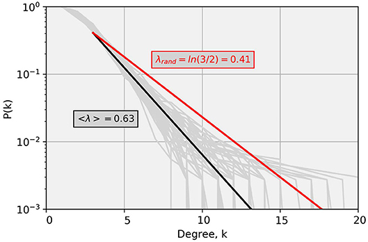
Figure 6. Illustration of degree distributions for the Cedar River at Cedar Rapids. Gray lines represent degree distributions for each year (daily values), while the solid black line represents the mean exponential fit, over entire years of record. The solid red line corresponds to the degree distribution associated with a purely random process. Note that basically for all years λ is > 0.41, indicating a consistent stochastic process.
To elucidate this further, consider the two-dimensional histogram plot in Figure 7. We show here values of λ and GC computed across all stations for all years pooled together. Each pixel represents the number of pairs (counts) of λ and GC. This plot clearly illustrates a strong relationship between λ and GC. We note that an increase of λ is (on average) followed by an increase of GC, which confirms a coupling (on average) between the values of λ and GC, as speculated above (see also Braga et al., 2016). All stations exhibit λ > λrand and virtually all values of GC > 0.345 (see Braga et al., 2016), suggesting that the streamflow process for the entire Iowa region at a daily time scale has its origin in the long-range correlated stochastic process. In other words, both measures can aptly reveal the stochastic nature of the underlying streamflow process and the associated potential predictability at a daily time scale. Because this plot shows overall dynamics of the process, it might not sufficiently illustrate the temporal evolution of each of these measures. Therefore, we discuss this aspect of λ and GC in more detail in the next section.
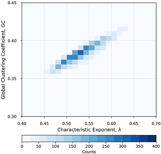
Figure 7. Two-dimensional histogram plot showing a strong relationship between characteristic exponent, λ, and global clustering coefficient, GC, for all stations and all years pooled together. The color code represents the number of pairs of λ and GC values in any pixel. It is apparent that all stations exhibit λ > λrand = 0.41. Virtually all values of GC > 0.345 (Braga et al., 2016), suggesting that the streamflow process for the entire Iowa region at a daily time scale has its origin in the long-range correlated (persistence) stochastic process. Note that as λ increases, GC also increases, as expected when the process becomes more and more linear.
Analysis of Raw Streamflow Time Series
A rationale behind using normalized streamflow time series is to avoid potential seasonal trends in streamflow (see Braga et al., 2016; Serinaldi and Kilsby, 2016; Lange et al., 2018). Here, we performed a similar analysis for λ and GC using raw streamflow time series. In Figure 8, we present two-dimensional histograms with a 1:1 relationship between metrics for raw and normalized streamflow for the pooled data for the state. The distribution of λ around the 1:1 line is almost symmetric as depicted by the percentage of pooled data. It illustrates that λ derived from an HVG-based network (see Figure 8A) is not overly sensitive to the normalization of streamflow, at least at the daily time scale (47 vs. 53% of the total number of data points toward normalized and raw data, respectively). In Figure 8B, we show the histogram for GC between normalized and raw streamflow data. Unlike λ, GC shows a strong bias toward the normalized data (99% of the total number of data points). As can be seen from the figure, the dynamic range of GC is much smaller compared to λ. The disparity in our inference from GC arises mainly from the disparity in complex internal structures of the network for the two forms of streamflow time series (see Figure 9). Figure 9 shows an example of the difference in network structure for the Cedar River at Cedar Rapids for 1904 and 2016. The natural streamflow data for 1904 (see Figure 9B) shows significant departure in the network internal structure from 2016 (see Figure 9A), mainly due to dominant base flow conditions in the network. Consequently, λ is enhanced while GC shows decline because the internal structure of the network is simplified. This is reflected in a large majority of GC obtained from raw streamflow depicting a chaotic regime. At the least, this is illustrative of the fact that GC is more sensitive to the form of streamflow data in assessing the streamflow predictability based on HVG-derived networks.
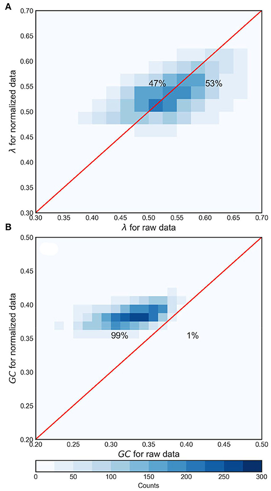
Figure 8. Two-dimensional histogram depicting the comparison between metrics for normalized and raw streamflow time series. The metrics are pooled from all stations for all historical records. (A) Comparison of λ and (B) comparison of GC. As explained in the text, GC is more affected by normalization than λ, with higher values for the normalized data (99% of the data points favoring normalized data), indicating that normalization tends to result in more connected networks, hence, more linear processes.
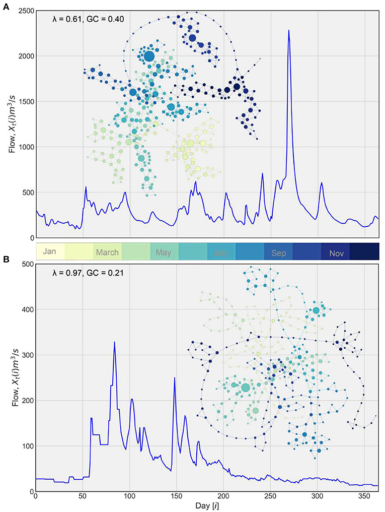
Figure 9. Illustration of networks corresponding to natural streamflow time series for the Cedar River at Cedar Rapids station. The color code corresponds to the month of the time series while the size of nodes corresponds to the number of connections they have with other nodes. (A) Network for 2016. (B) Network for 1904.
Analysis of the Effect of Time Scale of Streamflow Time Series
We want to exploit the utility of instantaneous (sampled every 15 min) streamflow data, especially in the context of streamflow forecasting. Therefore, we devised an experiment to explore the variability of the predictability measure λ and GC across three time scales (15 min, 1 h, and 1 day) using the same setup as described earlier for the daily time scale streamflow time series with the entire historical record. Note that we used the normalized streamflow for all three scales.
In Figure 10A, we use violin plots to present the variability of λ across the three time scales. An attractive feature of violin plots is their ability to show the estimated kernel density of points in addition to typical measures of variability depicted in box plots (e.g., Hintze et al., 1998; Jadidoleslam et al., 2019). The plots show that the variability of λ in terms of interquartile range (thicker dark solid line inside each violin) does not differ much across time scales. However, the major difference is in terms of the median values of λ. Clearly, the mean and median values of λ show the increase as we transition to a longer time scale. The mean and median λ fall marginally below λrand limit, showing that there is a tendency to transition to chaotic dynamics from stochastic dynamics as we move to finer resolution. In other words, the predictability of streamflow process is sensitive to the time scale of streamflow time series. Figure 10B shows similar behavior across time scales for GC. The mean and median GC increase as we increase the time scale. The GC, however, shows the reduction in the variability as the averaging time scale increases, which was not as apparent with λ.
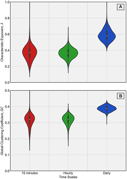
Figure 10. Violin plots of λ and GC across time scales of streamflow time series in (A,B), respectively. The solid white dot inside each violin represents median while the thicker solid line inside represents interquartile range (75th percentile−25th percentile). Clearly, the daily time scales have higher λ and higher GC, indicating that averaging affects the dynamics (from chaotic at short time scales to stochastic at longer time scales).
To elucidate it further, we performed similar analysis using a resampling approach across time scales. In addition to the three time scales discussed above, we added 3-, 6-, and 12-h resampling intervals to our analysis. Both λ and GC show systematic transition toward stochastic dynamics as the resampling interval approaches 1 day from 1 h, which is consistent with the result from averaging of 15-min streamflow data (see Supplementary Material, Figure A1). Note that the clear transition to a stochastic process occurs at the 6-h scale irrespective of whether a resampling or averaging method is used.
Spatial and Temporal Dependence of λ
From a hydrologic standpoint, it is important to understand the predictability of streamflow process across spatial scales. In Figure 11, we illustrate the relationship between λ and basin scale. Figure 11A depicts a clear spatial dependence of 〈λ〉 emerging from the daily scale streamflow time series. The solid black line represents a regression model fit using power law which shows that the variability in streamflow predictability in terms of λ is explained by the basin scales. For detailed visualization of uncertainty in λ conditional on basin scales, we present violin plots in Figure 11B. The uncertainty arises from variability over the historical periods of records conditional on windows of basin scales. Most of the point density of λ is around the median, depicting a similar relationship as Figure 11A. Clearly, the larger the basin scales, the longer the persistent behavior of streamflow (also see Ghimire and Krajewski, 2020) and hence the predictability of streamflow. This is supported by the fact that larger basin scales have been shown to display long memory.
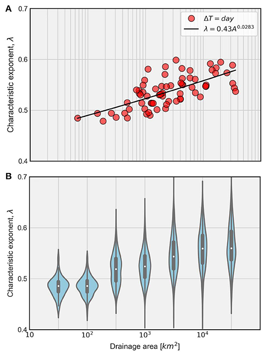
Figure 11. Spatial dependence of λ. (A) Expected value of λ over the years across stations. The solid dark line corresponds to the power-law model fit to the data. The relationship between expected value of λ and drainage area is statistically significant. (B) Distribution of λ over the years considering pooled data from consecutive windows of basin scales. Clearly, the size of drainage area affects the resulting processes. The larger the basin scales, the longer the persistent behavior of streamflow.
In the Supplementary Material (Figure A2), we present spatial dependence of λ across five time scales using a resampling approach. It is interesting to see the consistent transition between λ and basin size as the resampling time interval increases. For the sake of brevity, we do not show here results from averaging time scales, but they are very similar. In the Supplementary Material (Figure A3), we show similar plots for the raw streamflow data. The apparent difference between these two results is at 1- and 3-h time intervals. The values of λ at small basins show further decline while they increase for larger basins. If interpreted in conjunction with the Supplementary Material (Figure A4), the normalization at larger basin sizes shows the effect of measurement noise among other sources of uncertainty in λ, while small basins show the strong imprint of non-linearity from rainfall. This result has important implications for water resources management and skillful streamflow (flood) forecasting.
In addition, it is of interest to the forecasting community to assess whether the streamflow predictability measures λ and GC change over time. Due to their longer records, we use daily data in this analysis. Hypothesizing that such changes would be gradual, we fit a simple linear regression model for each measure against time t [years]. For λ, the model we fit is of the form:
where aλ and bλ are intercept and slope of the model fit line, respectively. Subsequently, we fit a similar model as Equation 5 to GC of the form:
where aGC and bGC are intercept and slope parameters of linear model fit, respectively, employing ordinary least squares method. Figure 12 shows spatial distribution of stations with temporal trend of predictability measures λ and GC. The circles that are both blue and red correspond to the stations with statistically significant values of bλ and bGC at 95% confidence level. In other words, 17 stations show a significant temporal trend of both λ and GC. The solid blue and solid red circles represent stations with a significant temporal trend of either λ or GC alone, respectively. Figure 12 shows that both measures depict a temporal trend at a similar number of collocated stations across the state. Therefore, data from 28 out of 64 stations show statistically significant trends. Insets (A) and (B) show examples of stations with and without a significant temporal trend of λ, respectively. Though the assumption of residuals distribution being normal is not valid in this case, studies have shown that using the bootstrap regression also yields similar results (Braga et al., 2016). Moreover, a large majority of these stations are of scales larger than 1,000 km2, which suggests that a temporal trend of streamflow predictability is more prominent at larger basin scales. Further, it is apparent in the central-eastern parts of the state, which could be attributed to factors such as anthropogenic (tiling) and/or climatic changes. The explicit attribution of temporal trends is beyond the scope of this study.
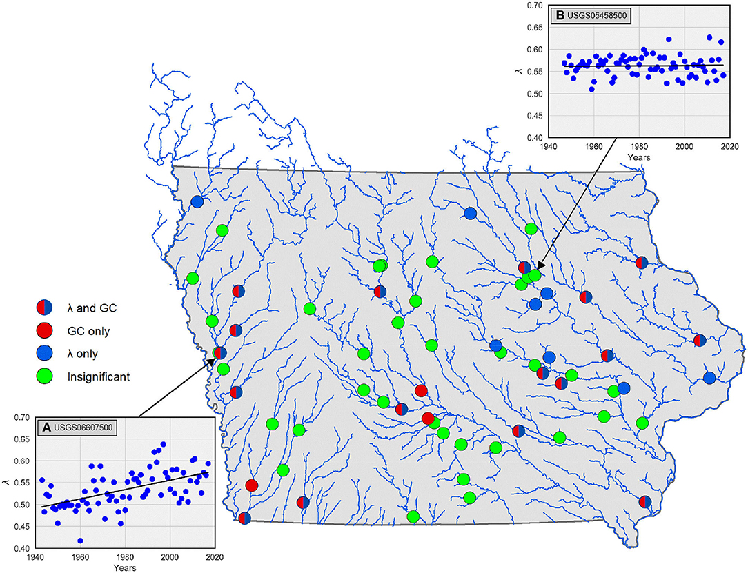
Figure 12. Illustration of USGS sites with statistically significant temporal trends of streamflow predictability. The solid blue circles represent stations with evolutive trend in terms of λ only; solid red circles represent stations with evolutive trend in terms of GC only; circles that are both red and blue represent stations with evolutive trend in terms of both λ and GC; light green circles do not show any trend. Insets (A,B) are examples of scatterplots with and without significant temporal trends, respectively.
Summary and Conclusions
We explored streamflow predictability across scales using 64 stations in the state of Iowa and gained insights by distinguishing between underlying stochastic and chaotic processes. The main tools of our analysis were characteristics of complex networks constructed from HVG. We estimated the characteristic exponent, λ, from degree distributions of network nodes and the global clustering coefficient, GC, across spatial basin scales and in time. Our study answers some key questions set forth at the beginning of this paper pertaining to fundamentals of predictability of streamflow process from the hydrologic standpoint.
• We showed that determining the predictability of streamflow process lies in the distinction between chaotic and stochastic processes. Our results based on HVG application to streamflow at a daily time scale demonstrate that streamflow dynamics is a correlated stochastic process. The presence of correlated structure in streamflow dynamics indicates the potential for strong predictability of streamflow.
• The normalization of streamflow shows strong effect on the overall inference on predictability. We show that GC is more sensitive than λ to the form of streamflow data. The values of GC show a transition of dynamics regime in a large majority of networks (stations and years). These findings show that normalized streamflow time series is better suited for such analyses considering the existence of seasonal effects inherent in streamflow process.
• Our results in terms of λ and GC for normalized streamflow across three time scales (e.g., 15 min, 1 h, and 1 day) show the increase in λ and GC as we transition to longer time scales. The mean and median λ fall marginally below λrand, showing that there is a tendency to transition to chaotic dynamics from stochastic dynamics at the short time scale and instantaneous sampling without temporal averaging. We attribute this change in streamflow predictability across time scales to changes in the dynamics of the process itself as we average it over time.
• For the hydrologic community, it is of interest to understand the predictability of streamflow process across spatial scales. We show a clear spatial scale dependence of λ for streamflow at the daily time scale. The larger the basin scales, the longer the persistent behavior of streamflow and, hence, the predictability of streamflow. Small basins show a chaotic behavior when analyzed using instantaneous data, i.e., the raw dynamics. These results have important implications for real-time streamflow forecasting and water resources management. They confirm the commonly known fact that flash floods are more difficult to forecast than riverine flooding that evolves slower in time. The chaotic signature in the streamflow dynamics at small scales is likely a consequence of chaos in the rainfall (see Rodriguez-Iturbe et al., 1989; Tsonis et al., 1993). At large scales, the effect of rainfall is moderated by the water transport in the river network that represents mostly aggregations, i.e., a nearly linear process.
• Finally, the forecasting community is always interested in assessing the temporal trend of streamflow predictability. A simple linear regression-based evolution model fit shows that 31 stations show a statistically significant trend in terms of λ while 26 stations show statistically a significant trend in terms of GC. The changes could have arisen from factors such as climate change-induced activities, changing rainfall patterns, and land-use patterns. The explicit attribution of the trends requires further research focusing solely on their impact to predictability of streamflow process.
As rainfall is the key agent of flooding in Iowa, it should be interesting to explore the effect of rainfall on predictability of streamflow. At small scales, rainfall and streamflow are connected more strongly than at large scales, where water transport separates the two. Water transport is in the river network where streamflow aggregation process plays an important role in shaping streamflow fluctuations (e.g., Ayalew et al., 2014a,b, 2015). The connection of streamflow predictability to other hydrologic processes is known to exist (Wood et al., 2016; Arnal et al., 2017; Harrigan et al., 2018). Streamflow predictability has been shown to rely upon the land surface (e.g., catchment) memory, and the persistence in the land surface initial hydrologic conditions (e.g., soil moisture, groundwater, existing streamflow, and snowpack). Initial hydrologic conditions are the major sources of predictability of streamflow and are typically considered the starting point for any long-range streamflow forecasting system (Wood et al., 2016; Arnal et al., 2017). The achievable predictability of streamflow has shown dependency with the season (the transition between dry and wet seasons), the individual catchment location and size (e.g., the streamflow in a large basin with a slow response time and negligible precipitation are easier to forecast, which our study also indicated), and storage properties (e.g., Arnal et al., 2017; Harrigan et al., 2018).
We did not analyze the effects of streamflow measurement errors as the USGS data are considered to be accurate within 5% (e.g., Ghimire and Krajewski, 2020). For our analysis, we expect the measurement uncertainty to have minimal impact on the overall inference. We performed a fundamental study on the predictability of the streamflow process through HVG-based complex networks. We believe our findings provide a hydrologic context of interpreting the underlying dynamics of the streamflow process. Our analysis captures a wide range of spatial scales; hence, results are deemed adequate in representing hydrologic processes across scales. We need to stress here that, insofar as λ is a discriminant between a chaotic process and a stochastic (correlated) process, and insofar as GC is found to relate toλ, this study indirectly explores non-linearity in streamflow, regardless of not finding evidence for it. Exploiting this aspect of streamflow process and its impact on predictability, and incorporating that in our hydrologic modeling strategy, is open to further and future research.
Though we implemented our analysis to Iowa, we think that the streamflow process will demonstrate similar predictability across scales in regions with similar landscapes and climatology, such as the Upper Mississippi and Ohio River basins (e.g., Schilling et al., 2015) when derived from HVG-based complex networks. Given that the hydro-climatologic conditions, landscapes, and base flow conditions are quite similar, the inference on streamflow dynamics across spatio-temporal scales is expected to be similar. Though we did not report it in this paper, one could separately perform the effect of time resolution (time scale) on standard chaotic maps, which could validate our results in a standalone approach.
Data Availability Statement
The datasets generated for this study are available on request to the corresponding author.
Author Contributions
All authors listed have made a substantial, direct and intellectual contribution to the work and approved it for publication.
Funding
The authors acknowledge the support from the Iowa Flood Center and the IIHR-Hydroscience and Engineering and the University of Iowa. WK acknowledges partial support of the Rose and Joseph Summers endowment. NJ was supported by the NASA's Science Utilization of the Soil Moisture Active-Passive Mission program grant NNX16AQ57G.
Conflict of Interest
The authors declare that the research was conducted in the absence of any commercial or financial relationships that could be construed as a potential conflict of interest.
Acknowledgments
The authors acknowledge the computational support from the High-Performance Computing group at the University of Iowa.
Supplementary Material
The Supplementary Material for this article can be found online at: https://www.frontiersin.org/articles/10.3389/frwa.2020.00017/full#supplementary-material
See Supplemental Material for four additional figures exploring the effect of time scales on λ and GC and their spatial scale dependence. Figure A1 shows the relationship between λ and GC across resampling time scales of 1, 3, 6, 12, and 24 h. Figure A2 depicts spatial variability of λ across these time scales as obtained from a resampling approach. Figure A3 depicts the similar relationship between λ and basin sizes for raw streamflow data. Figure A4 is a demonstration of how averaging and resampling change the streamflow dynamics for raw and normalized streamflow data across two basin sizes of 500 km2 and 16,800 km2.
References
Albert, R., and Barabási, A. L. (2002). Statistical mechanics of complex networks. Rev. Mod. Phys. 74, 47–97. doi: 10.1103/RevModPhys.74.47
Arnal, L., Wood, A. W., Stephens, E., Cloke, H. L., and Pappenberger, F. (2017). An efficient approach for estimating streamflow forecast skill elasticity. J. Hydrometeorol. 18, 1715–1729. doi: 10.1175/JHM-D-16-0259.1
Ayalew, T. B., Krajewski, W. F., and Mantilla, R. (2014a). Connecting the power-law scaling structure of peak-discharges to spatially variable rainfall and catchment physical properties. Adv. Water Resour. 71, 32–43. doi: 10.1016/j.advwatres.2014.05.009
Ayalew, T. B., Krajewski, W. F., and Mantilla, R. (2015). Analyzing the effects of excess rainfall properties on the scaling structure of peak discharges: insights from a mesoscale river basin. Water Resour. Res. 51, 3900–3921. doi: 10.1002/2014WR016258
Ayalew, T. B., Krajewski, W. F., Mantilla, R., and Small, S. J. (2014b). Exploring the effects of hillslope-channel link dynamics and excess rainfall properties on the scaling structure of peak-discharge. Adv. Water Resour. 64, 9–20. doi: 10.1016/j.advwatres.2013.11.010
Bordignon, S., and Lisi, F. (2000). Nonlinear analysis and prediction of river flow time series. Environmetrics 11, 463–477. doi: 10.1002/1099-095X(200007/08)11:4<463::AID-ENV429>3.0.CO;2-#
Braga, A. C., Alves, L. G. A., Costa, L. S., Ribeiro, A. A., De Jesus, M. M. A., Tateishi, A. A., et al. (2016). Characterization of river flow fluctuations via horizontal visibility graphs. Phys. A Stat. Mech. Appl. 444, 1003–1011. doi: 10.1016/j.physa.2015.10.102
Casdagli, M. C., and Weigend, A. S. (1993). Exploring the Continuum Between Deterministic and Stochastic Modeling, in Time Series Prediction: Forecasting the Future and Understanding the Past. eds A. Weigend, and N. A. Gershenfeld (Boston, MA: Addison-Wesley).
Costa, L. D. F., Rodrigues, F. A., Travieso, G., and Boas, P. R. V. (2007). Characterization of complex networks: a survey of measurements. Adv. Phys. 56, 167–242. doi: 10.1080/00018730601170527
Coulibaly, P., and Burn, D. H. (2004). Wavelet analysis of variability in annual Canadian streamflows. Water Resour. Res. 40:667. doi: 10.1029/2003WR002667
Ghimire, G. R., and Krajewski, W. F. (2020). Exploring persistence in streamflow forecasting. J. Am. Water Resour. Assoc. 56, 542–550. doi: 10.1111/1752-1688.12821
Ghimire, G. R., Krajewski, W. F., and Mantilla, R. (2018). A Power law model for river flow velocity in Iowa basins. J. Am. Water Resour. Assoc. 54:665. doi: 10.1111/1752-1688.12665
Gonçalves, B. A., Carpi, L., Rosso, O. A., and Ravetti, M. G. (2016). Time series characterization via horizontal visibility graph and information theory. Phys. A Stat. Mech. Appl. 464, 93–102. doi: 10.1016/j.physa.2016.07.063
Grassberger, P., and Procaccia, I. (1983). Characterization of strange attractors. Phys. Rev. Lett. 50, 346–349. doi: 10.1103/PhysRevLett.50.346
Harrigan, S., Prudhomme, C., Parry, S., Smith, K., and Tanguy, M. (2018). Benchmarking ensemble streamflow prediction skill in the UK. Hydrol. Earth Syst. Sci. 22, 2023–2039. doi: 10.5194/hess-22-2023-2018
Hintze, J. L., Nelson, R. D., Hintze, J. L., and Nelson, R. D. (1998). Taylor & Francis, Ltd. Am. Statis. Associat. 52, 181–184. doi: 10.2307/2685478
Jadidoleslam, N., Mantilla, R., Krajewski, W. F., and Goska, R. (2019). Investigating the role of antecedent SMAP satellite soil moisture, radar rainfall and MODIS vegetation on runoff production in an agricultural region. J. Hydrol. 579:4210. doi: 10.1016/j.jhydrol.2019.124210
Koutsoyiannis, D. (2006). On the quest for chaotic attractors in hydrological processes. Hydrol. Sci. J. 51, 1065–1091. doi: 10.1623/hysj.51.6.1065
Kumar, P. (2011). Typology of hydrologic predictability. Water Resour. Res. 47, 1–9. doi: 10.1029/2010WR009769
Lacasa, L., Luque, B., Ballesteros, F., Luque, J., and Nuño, J. C. (2008). From time series to complex networks: the visibility graph. Proc. Natl. Acad. Sci. U.S.A. 105, 4972–4975. doi: 10.1073/pnas.0709247105
Lacasa, L., Nuñez, A., Roldán, É., Parrondo, J. M. R., and Luque, B. (2012). Time series irreversibility: a visibility graph approach. Eur. Phys. J. B 85:217. doi: 10.1140/epjb/e2012-20809-8
Lacasa, L., and Toral, R. (2010). Description of stochastic and chaotic series using visibility graphs. Phys. Rev. E Stat. Nonlinear Soft Matter Phys. 82:120. doi: 10.1103/PhysRevE.82.036120
Lange, H., Sippel, S., and Rosso, O. A. (2018). Nonlinear dynamics of river runoff elucidated by horizontal visibility graphs. Chaos An Interdiscip. J. Nonlinear Sci. 28:75520. doi: 10.1063/1.5026491
Livina, V., Ashkenazy, Y., Kizner, Z., Strygin, V., Bunde, A., and Havlin, S. (2003). A stochastic model of river discharge fluctuations. Phys. A Stat. Mech. Appl. 330, 283–290. doi: 10.1016/j.physa.2003.08.012
Lundquist, J. D., and Cayan, D. R. (2002). Seasonal and spatial patterns in diurnal cycles in streamflow in the western United States. J. Hydrometeorol. 3, 591–603. doi: 10.1175/1525-7541(2002)003<0591:SASPID>2.0.CO;2
Luque, B., Lacasa, L., Ballesteros, F., and Luque, J. (2009). Horizontal visibility graphs: exact results for random time series. Phys. Rev. E Stat. Nonlinear Soft Matter Phys. 80:103. doi: 10.1103/PhysRevE.80.046103
Newman, M. E. J. (2003). The structure and function of complex networks. SIAM Rev. 45, 167–256. doi: 10.1137/S003614450342480
Pasternack, G. B. (1999). Does the river run wild? Assessing chaos in hydrological systems. Adv. Water Resour. 23, 253–260. doi: 10.1016/S0309-1708(99)00008-1
Porporato, A., and Ridolfi, L. (1997). Nonlinear analysis of river flow time sequences. Water Resour. Res. 33, 1353–1367. doi: 10.1029/96WR03535
Prairie, J. R., Rajagopalan, B., Fulp, T. J., and Zagona, E. A. (2006). Modified K-NN model for stochastic streamflow simulation. J. Hydrol. Eng. 11, 371–378. doi: 10.1061/(ASCE)1084-0699(2006)11:4(371)
Prokhorenkova, O., and Samosvat, E. L. (2014). Global clustering coefficient in scale-free networks. Intern. Workshop Algorithms Models Web-Graph 47:58. doi: 10.1007/978-3-319-13123-8_5
Rodriguez-Iturbe, I., Febres De Power, B., Sharifi, M. B., and Georgakakos, K. P. (1989). Chaos in rainfall. Water Resour. Res. 25, 1667–1675. doi: 10.1029/WR025i007p01667
Schilling, K. E., Wolter, C. F., and McLellan, E. (2015). Agro-hydrologic landscapes in the upper Mississippi and Ohio river basins. Environ. Manage. 55, 646–656. doi: 10.1007/s00267-014-0420-x
Serinaldi, F., and Kilsby, C. G. (2016). Irreversibility and complex network behavior of stream flow fluctuations. Phys. A Stat. Mech. its Appl. 450, 585–600. doi: 10.1016/j.physa.2016.01.043
Smith, L. C., Turcotte, D. L., and Isacks, B. L. (1998). Stream flow characterization and feature detection using a discrete wavelet transform. Hydrol. Process. 12, 233–249.
Stephen, M., Gu, C., and Yang, H. (2015). Visibility graph based time series analysis. PLoS ONE 10:e0143015. doi: 10.1371/journal.pone.0143015
Tsonis, A. A., and Elsner, J. B. (1992). Nonlinear prediction as a way of distinguishing chaos from random fractal sequences. Nature 358, 217–220. doi: 10.1038/358217a0
Tsonis, A. A., Elsner, J. B., and Georgakakos, K. P. (1993). Estimating the dimension of weather and climate attractors: important issues about the procedure and interpretation. J. Atmos. Sci. 50, 2549–2555. doi: 10.1175/1520-0469(1993)050<2549:ETDOWA>2.0.CO;2
Tsonis, A. A., and Roebber, P. J. (2004). The architecture of the climate network. Phys. A Stat. Mech. Appl. 333, 497–504. doi: 10.1016/j.physa.2003.10.045
Tsonis, A. A., Swanson, K. L., and Roebber, P. J. (2006). What do networks have to do with climate? Bull. Am. Meteorol. Soc. 87, 585–595. doi: 10.1175/BAMS-87-5-585
Wang, W. (2006). Stochasticity, Nonlinearity and Forecasting of Streamflow Processes. Amsterdam: IOS Press.
Watts, D. J., and Strogatz, S. H. (1998). Collective dynamics of “small-world” networks. Nature 393, 440–442. doi: 10.1038/30918
Wood, A. W., Pagano, T., and Roos, M. (2016). Tracing The Origins of ESP. HEPEX Blog. Available online at: https://hepex.inrae.fr/tracing-the-origins-of-esp/ (accessed July 07, 2020).
Keywords: streamflow dynamics, complex networks, horizontal visibility graph, degree distribution, streamflow predictability
Citation: Ghimire GR, Jadidoleslam N, Krajewski WF and Tsonis AA (2020) Insights on Streamflow Predictability Across Scales Using Horizontal Visibility Graph Based Networks. Front. Water 2:17. doi: 10.3389/frwa.2020.00017
Received: 31 October 2019; Accepted: 16 June 2020;
Published: 23 July 2020.
Edited by:
Bhavna Arora, Lawrence Berkeley National Laboratory, United StatesReviewed by:
Xianhong Xie, Beijing Normal University, ChinaXi Chen, University of Cincinnati, United States
Copyright © 2020 Ghimire, Jadidoleslam, Krajewski and Tsonis. This is an open-access article distributed under the terms of the Creative Commons Attribution License (CC BY). The use, distribution or reproduction in other forums is permitted, provided the original author(s) and the copyright owner(s) are credited and that the original publication in this journal is cited, in accordance with accepted academic practice. No use, distribution or reproduction is permitted which does not comply with these terms.
*Correspondence: Ganesh R. Ghimire, Z2FuZXNoLWdoaW1pcmVAdWlvd2EuZWR1