Downscaling Satellite and Reanalysis Precipitation Products Using Attention-Based Deep Convolutional Neural Nets

High-quality and high-resolution precipitation products are critically important to many hydrological applications. Advances in satellite remote sensing instruments and data retrieval algorithms continue to improve the quality of the operational precipitation products. However, most satellite products existing today are still too coarse to be ingested for local water management and planning purposes. Recent advances in deep learning algorithms enable the fusion of multi-source, high-dimensional data for statistical learning. In this study, we investigated the efficacy of an attention-based, deep convolutional neural network (AU-Net) for learning spatial and temporal mappings from coarse-resolution to fine-resolution precipitation products. The skills of AU-Net models, developed using combinations of static and dynamic predictors, were evaluated over a 3 × 3° study area in Central Texas, U.S., a region known for its complex precipitation patterns and low predictability. Three coarse-resolution satellite/reanalysis precipitation products, ERA5-Land (0.1°), TRMM (0.25°), and IMERG (0.1°), are used as part of the inputs, while the predictand is the 1-km PRISM data. Auxiliary predictors include elevation, vegetation index, and air temperature. The study period includes 18 years of data (2001–2018) at the monthly scale for training, validation, and testing. Results show that the trained AU-Net models achieve different degrees of success in downscaling the baseline coarse-resolution products, depending on the total precipitation, the accuracy of large-scale patterns captured by the baseline products, and the amount of information transferable from predictors. Higher precipitation rate tends to affect AU-Net model performance negatively. Use of the attention mechanism in the AU-Net models allows for infilling of multiscale features and generation of sharper images. Correction using gauge data, if there is any, can further improve the results significantly.

1. Introduction

Precipitation is a primary driver of water and energy cycle (Trenberth et al., 2007), providing essential inputs to many water, food, and energy applications including, but not limited to, global and regional climate variability assessments, land surface-atmosphere interactions, natural hazard prevention, crop yield management, hydrological forecasting, and surface and groundwater resources planning (Hong et al., 2007; Seneviratne et al., 2010; Becker et al., 2013; Schewe et al., 2014). To a large degree, the effectiveness of many disaster response and water resources management decisions hinge on the quantity and quality, as well as the spatial and temporal resolution of precipitation products. Currently available precipitation products may be classified into ground-based, satellite-based, reanalysis, and hybrid multi-source/multi-sensor products.

Ground-based products are derived from rain gauges and weather radar. However, the spatial coverage of rain gauge networks is often limited, also varying significantly across different countries owing to temporal sampling resolutions, periods of operation, data latency, and data access (Kidd et al., 2017). At the global scale, ground-based products are only available at a relatively coarse resolution (≥0.5°) and updated rather infrequently (Sun Q. et al., 2018). High-resolution gridded products are only available in a few developed counties that have extensive gauge network coverage. For example, in the U.S., the Parameter-elevation Regressions on Independent Slopes Model (PRISM) gauge-based product (4-km resolution, 1895–present), developed by the Oregon State University (Daly et al., 1997), is widely used for operational planning and validation of satellite products. Similarly, the Stage IV radar-based, gauge-adjusted precipitation data (4 km, 2002–present) available from the National Center for Environmental Prediction (NCEP) is also commonly used as a reference dataset in many conterminous U.S. (CONUS) precipitation product comparisons (Lin and Mitchell, 2005).

Satellite precipitation products are derived from passive and active microwave (MW) sensors onboard low Earth orbiting satellites, and visible/infrared (VIS/IR) sensors onboard geostationary satellites (Hou et al., 2014). So far, the raw satellite precipitation data has been mainly retrieved from three spaceborne precipitation radars: the Ku-band precipitation radar onboard the Tropical Rainfall Measuring Mission (TRMM) satellite that was in orbit from 1997 to 2015, the W-band Cloud Profiling Radar (CPR) onboard the CloudSat operating from 2006 to the present, and the Dual-frequency Precipitation Radar (DPR) onboard the Global Precipitation Measurement (GPM) Core Observatory operating from 2014 to the present (Tang et al., 2018b). Unlike ground-based products, satellite products provide spatially homogeneous coverage with low latency. Some of the currently available satellite products, such as the Integrated Multi-satellite Retrievals for GPM (IMERG) (Huffman et al., 2015) and TRMM Multi-satellite Precipitation Analysis (Huffman et al., 2007), not only assimilate information from multiple MW/IR sensors, but also are corrected by ground observations. Currently, the most common resolution of satellite precipitation products is 0.25° per 3 h (Sun Q. et al., 2018).

Reanalysis products are generated by assimilating irregular observations into earth system models to generate a synthesized estimate of the state of the system (e.g., precipitation) across a uniform model grid, with spatial homogeneity and temporal continuity (Sun Q. et al., 2018). The commonly used reanalysis products include the NCEP/NCAR Reanalysis system (1.875°, 1979–2010) (Kistler et al., 2001), European Center for Medium-Range Weather Forecasts (ECMWF) reanalysis systems (0.25/0.75°, 1979–present) (Dee et al., 2011), and the NCEP Climate Forest System Reanalysis system (CFSR, 38 km, 1979–2010) (Saha et al., 2010).

Recent trends in precipitation product development are geared toward merging multi-source and multi-sensor data to leverage information existing at multiple scales. Examples include the Multi-Source Weighted-Ensemble Precipitation (MSWEP, 0.1/0.5°, 1979–present) (Beck et al., 2017) and Modern-Era Retrospective Analysis for Research and Application system (MERRA-2) (Rienecker et al., 2011), both combining gauge, satellite, and reanalysis data. These products typically adopt an optimal weighting scheme to merge information. In MSWEP, for example, weights assigned to the gauge-based data are determined from the gauge network density, while weights assigned to the satellite and reanalysis-based estimates are calculated from their comparative performance at the surrounding gauges (Beck et al., 2017).

Notwithstanding the tremendous effort dedicated to developing various products, precipitation forcing remains a major source of uncertainty in global hydrological and land surface models (Wood et al., 2011; Scanlon et al., 2018) because of its inherent high variability in space and time, especially in topographically complex, convection-dominated, and snow-dominated regions (Tang et al., 2018a; Beck et al., 2019). The accuracy of rain gauge data may be affected by a number of environmental factors, such as wind, wetting and evaporation loss, and undercatch (Sun Q. et al., 2018; Tang et al., 2018a). The uncertainty in satellite precipitation data may stem from different sources, including algorithms used for retrieving, downscaling, and merging multi-sensor data, as well as from the acquisition instrument itself (Sorooshian et al., 2011).

Recently, Sun Q. et al. (2018) reviewed 30 currently available global precipitation datasets, including gauge-based, satellite-related, and reanalysis datasets. They found that the magnitude of annual precipitation estimates over global land deviated by as much as 300 mm/yr among the products. They also noted that the degree of variability in precipitation estimates varied by region, with large differences found over tropical oceans, complex mountain areas, northern Africa, and some high-latitude regions. Beck et al. (2019) evaluated the performance of 26 gridded daily precipitation products over the CONUS for the period 2008–2017. Among the 15 uncorrected datasets considered, they found that ERA5-HRES (the 5th global reanalysis product released by ECMWF, 0.28°, 2008–present) gives better performance than others across most of CONUS, especially in the west; among the 11 gauge-corrected products, MSWEP V2.2 gives the best performance, which was attributed to applying daily gauge corrections and accounting for gauge reporting times during product development. Both product reviews suggest that the reliability of precipitation datasets depends on the number and spatial coverage of surface stations, the accuracy of satellite data retrieval algorithms, as well as the data assimilation models used. Most data assimilation and bias correction methods, in turn, rely on the understanding and characterization of precipitation error distributions, which are typically non-stationary and product dependent. AghaKouchak et al. (2012) investigated the systematic and random errors in several major satellite precipitation products against the NCEP Stage IV data. A major finding of their study is that the spatial distribution of the systematic error had similar patterns for all precipitation products they considered, for which the error is remarkably higher during the winter than in summer; the error was also found to be proportional to rain rates, with larger errors tending to be associated with higher rain rates. Parameterization of the precipitation error model is thus critically important for improving precipitation products, but remains a challenging task, partly because of the strong spatial and temporal variability in rainfall patterns (Sorooshian et al., 2011; AghaKouchak et al., 2012).

The advent of deep learning (DL) algorithms in recent years has revolutionized the field of statistical pattern recognition, enabling machines to achieve human-like classification accuracy (Goodfellow et al., 2016). Precipitation product development represents a research domain that can readily benefit from the DL because of the explosive growth of multiscale, multi-source Earth observation data (Ma et al., 2015; Sun and Scanlon, 2019). Pan et al. (2019) recently presented a convolutional neural network (CNN) method for precipitation estimation using numerical weather model outputs. The CNN model architecture follows an end-to-end design, in which a fully connected dense layer is used at the output layer to recover the dimensions of the input images. The input predictors they used include 3-h geopotential height and precipitable water at 500, 850, and 1,000 hPa, which were taken from the NCEP regional reanalysis at 32 km (~0.29°) resolution; and the predictand is the total precipitation. Their results show CNN obtained better skills in the northwest and east parts of CONUS, but performed poorer than the reference Climate Prediction Center (CPC) gauge-based dataset in the mid-U.S. Tang et al. (2018b) applied a four-layer, deep multilayer perceptron network to predict precipitation rates (at single locations), by mapping passive microwave data from GPM and MODerate resolution Imaging Spectroradiometer (MODIS) to spaceborne radar data. Kim et al. (2017) used ConvLSTM, a combination of convolutional neural nets and long short-term memory (LSTM) neural net (Shi et al., 2015), for precipitation nowcasting using weather radar data. Their results showed ConvLSTM was able to obtain better results than the simple linear regression method. Similarly, ConvLSTM was recently used for precipitation estimation based on atmospheric dynamical fields simulated by ERA-Interim (a predecessor of ERA5) (Miao et al., 2019).

Tremendous interests exist in using machine learning techniques for statistical precipitation downscaling, which has long been studied even before the DL era to refine coarse-resolution precipitation products and global climate model projections for local water management and hydrological modeling needs (Maraun et al., 2010; Jia et al., 2011; Duan and Bastiaanssen, 2013; Chen et al., 2018). To correct biases arising during downscaling, two types of traditional methods may be identified, quantile mapping (Li et al., 2010; Shen et al., 2014; Yang et al., 2016) and multiplicative/additive correction (or linear scaling) (Vila et al., 2009; Jakob Themeßl et al., 2011). In the realm of DL, Vandal et al. (2018) introduced DeepSD, which is a stacked superresolution CNN for statistical downscaling of climate and Earth system model simulations. In their experiments, Vandal et al. (2018) upsampled the 4-km PRISM data progressively to 1°, and then tried to restore the original high-resolution data by training a CNN model. He et al. (2016) used the random forest algorithm to downscale the precipitation forcing field used in North-American Land Data Assimilation System Project Phase 2 (NLDAS-2). Their main research question was whether the upsampled NLDAS-2 precipitation forcing (in spatial resolutions of 0.25, 0.5, and 1°) could be restored to its native resolution (0.125°) by using additional dynamic and static information (e.g., air temperature, wind speed, elevation, slope) as auxiliary inputs.

So far, however, few studies have attempted to directly map coarse-resolution precipitation products (e.g., satellite or reanalysis products) to fine-resolution, gauge-based precipitation products using DL. As mentioned previously, gauge products tend to have higher resolutions but are often created using proprietary data processing algorithms that may not be readily accessible to local users. Inconsistencies in data release times may also prevent end users from accessing the information when they need it the most. The main motivation of this research was thus to investigate a data-driven, DL-based statistical downscaling procedure by learning covariational patterns between the coarse- and fine-resolution precipitation products. A novel, attention-based, deep convolutional neural network model was adopted to help capture multiscale spatial and temporal patterns. Once trained, end users may apply the DL-based model to generate downscaled high-resolution precipitation maps using only coarse-resolution products, which are available operationally. Ultimately, such a DL-based downscaling procedure may be applied to regions without high resolution products through transfer learning, in which models trained for data-rich domains are “transferred” to inform models for data-sparse domains (Pan and Yang, 2009; Goodfellow et al., 2016; Jean et al., 2016; Sun and Scanlon, 2019). Like in all regression studies, a main hypothesis underneath this research is that certain spatial and temporal covariational patterns exist between the predictand and its predictors, which has been confirmed to a certain degree by previous validation studies (Beck et al., 2017), but is also shown to vary significantly across space and time (AghaKouchak et al., 2012), creating a major challenge for the pattern-based learning algorithms.

For demonstration, we focus on Central Texas, which is a region of low hydrometeorological predictability (AghaKouchak et al., 2012; Sun et al., 2014; Beck et al., 2019; Pan et al., 2019), and yet, is frequented by flooding and drought events (Lowrey and Yang, 2008; Long et al., 2013; Sun A. Y. et al., 2018). PRISM data is used as the high-resolution training target. The performance of three coarse-resolution satellite and reanalysis products, along with other auxiliary variables, are evaluated. This paper is organized as follows. Section 2 describes the study area and datasets used. Section 3 presents the design of the deep CNN model. Results are provided in section 4, followed by discussion and conclusions. For reference, a table of major abbreviations and acronyms used this paper is provided in the Appendix.

2. Study Area and Data Used

2.1. Study Area

Central Texas represents the fastest-growing region in the U.S. among metros with at least 1 million people (Austin Statesman, 2019). The region is also known for its severe precipitation events, resulting from a juxtaposition of meteorological factors, including moisture influx from the Gulf of Mexico, easterly wave moving across the area, and orographic uplift from the Balcones Escarpment (a physiographic feature of steep elevation gradient at the boundary between the Edwards Plateau and the Gulf Coast Plain) (Hirschboeck, 1987; Nielsen-Gammon et al., 2005; Lowrey and Yang, 2008; Sun A. Y. et al., 2018).

The area of study is a 3 × 3° region bounded between latitudes 29–32°N and longitudes 100–97°W (Figure 1). It encompasses two major Central Texas cities, Austin and San Antonio, as well as their surrounding regions. Central Texas is part of the Texas Hill Country, which is within the Edwards Plateau, a geographic region known by its rugged karstic terrains and thin top soils (Mace et al., 2000). Major land cover types include forest lands, rangeland, agricultural lands, urban, barren land, and wetlands (Omranian and Sharif, 2018). Elevation is highest (736 m) near the west boundary of the study area and gradually decreases toward the east boundary to 42 m (Figure 1A). Climate in the region is humid subtropical, and precipitation exhibits a distinctive bimodal pattern: spring is the wettest season, with April and May the wettest months; a secondary peak of rainfall occurs in September and October (Slade and Patton, 2003). Spatially, the annual rainfall in the 3 × 3° region ranges from 575 to 1,005 mm, which is the highest in the east and decreases toward the west (Figure 1B). Tropical cyclones (hurricanes and tropic storms) typically occur in late summer or early fall, bringing the largest amount of rainfall. Moreover, Balcones Escarpment acts as a major mechanism of localization and intensification of rainfall (Nielsen-Gammon et al., 2005).

FIGURE 1

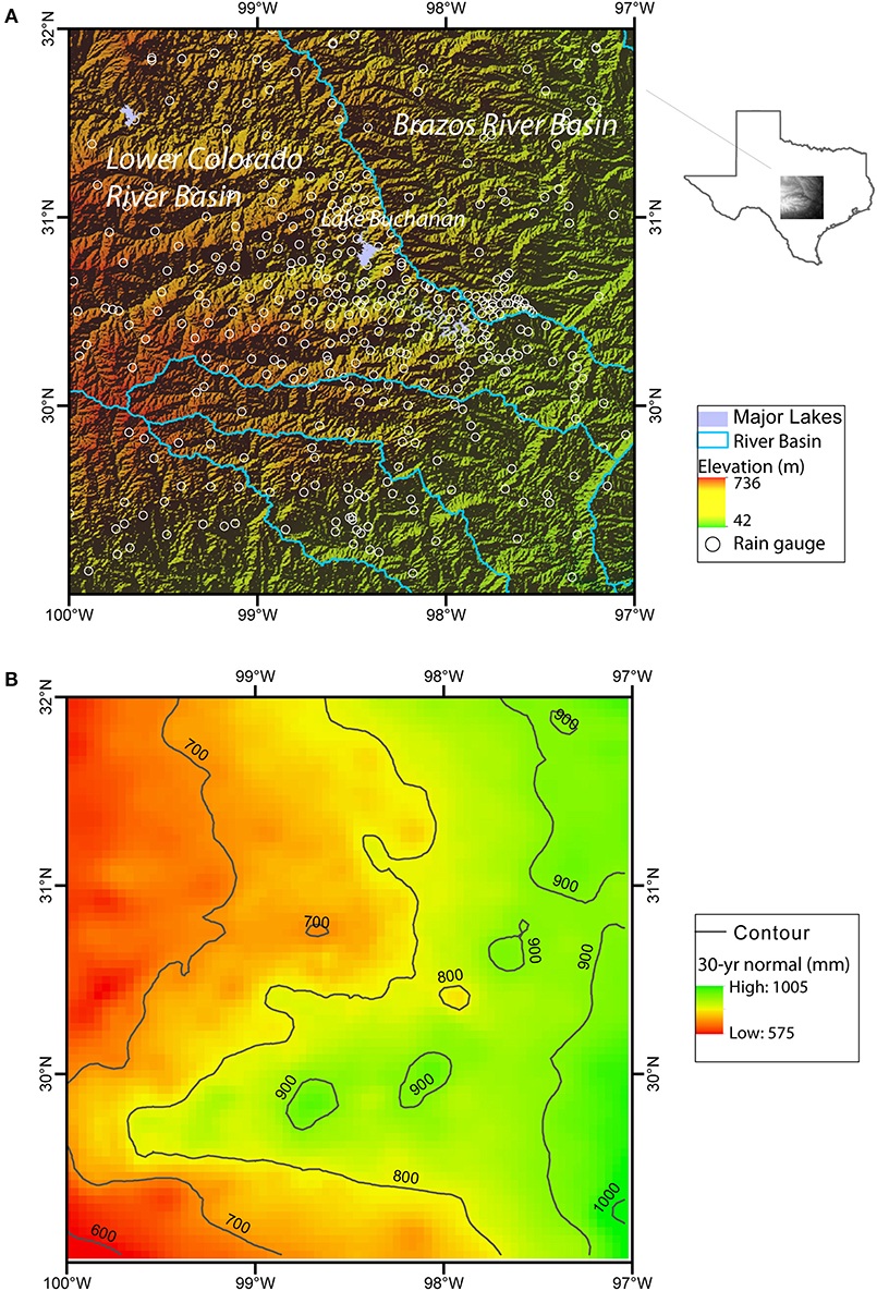
Figure 1. (A) Study area boundary (lat: 29–32°N, lon: 100–97°W) and the shaded relief map (open circles correspond to the existing rain gauges as of Jan 2017); (B) 30-years precipitation normal extracted from PRISM, where color and contour lines represent total rain amount in mm.

Hydrology wise, the study area is part of two major river basins, the Lower Colorado River Basin that drains to Lower Colorado River and its major tributaries (San Saba River, Llano River, and Pedernales River), and the Brazos River Basin. The former includes a cascade of surface reservoirs (e.g., Lake Buchanan, Lake Travis) that provide surface water supply to the City of Austin. In addition to flooding, severe drought is a major concern, often causing significant loss to the regional economy (Long et al., 2013). The accuracy and reliability of precipitation estimate is thus of paramount importance to local water agencies, for continuously evaluating flood/drought potential, as well as for quantifying groundwater recharge, reservoir storage, and water availability. For those reasons, the Lower Colorado River Authority (LCRA), the primary water management agency of the area, has established a dense gauge network in recent years to provide continuous rainfall data at relatively high spatial and temporal resolutions (open circles in Figure 1A). The in situ data offers important additional information for precipitation downscaling in this study, as discussed below in section 4.

2.2. Datasets

The study period is from Jan 2001 to Dec 2018, which was chosen based on the common period of coverage of all products considered. The monthly scale was chosen because of our interest in downscaling precipitation for supporting subseasonal water management activities. In the following, the gridded and gauge data used are described in details, and a summary of all data used is also provided in Table 1, including the data URLs.

TABLE 1

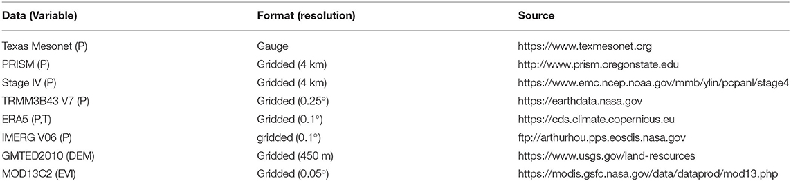
Table 1. Summary of datasets used in this study, where P–precipitation, T–temperature, DEM–elevation, EVI –enhanced vegetation index.

2.2.1. Gauge Data

Monthly gauge precipitation data was obtained from Texas Mesonet. Figure 1A shows the locations of rain gauges as of Jan 2017 (the first month of our test period), which are distributed more densely within the LCRA boundary than in the surrounding areas. The number of valid gauges increased from 361 in Jan 2017 to 532 in Dec 2018. As mentioned before, the number of rain gauges only increased in recent years in light of the severe 2012–2013 Texas drought. Before that event, the number of in situ data was generally much smaller. For example, the number of gauge data available in Jan 2003 was 24 and in Jan 2013 it was 53. Thus, the quality of the PRISM data evolved with time. In other words, patterns used for the training period may be less constrained than the patterns used during validation.

In this study, the gridded, gauge-based precipitation product PRISM is the training target or predictand. The Stage IV data from NCEP was used for cross-examining the PRISM patterns. Stage IV data includes merged operational radar data and rain gauge measurements in hourly accumulations. Both datasets have a spatial resolution of 4 km and were temporally aggregated to the monthly scale.

2.2.2. Satellite and Reanalysis Data

Three coarse-resolution satellite and reanalysis precipitation products, TRMM, ERA5-Land, and IMERG, were tested for generating PRISM like data. The TRMM data used in this study is 3B43 v7 (0.25°, 1998–2019), which is a post-real-time, gauge-corrected monthly product that merges precipitation estimates from multi-sensors, as well as monthly precipitation gauge analysis from the Global Precipitation Climatology Center (https://www.dwd.de) (see also Table 1). The main motivation behind developing the 3B43 algorithm was to produce the best estimate of precipitation rate from sensors onboard TRMM, as well as from other satellites including Advanced Microwave Scanning Radiometer for Earth Observing Systems (AMSR-E), Special Sensor Microwave Imager (SSMI), Special Sensor Microwave Imager/Sounder (SSMIS), Advanced Microwave Sounding Unit (AMSU), Microwave Humidity Sounder (MHS), and microwave-adjusted merged geo-infrared (IR) (Huffman et al., 2010). After TRMM was decommissioned in 2015, TRMM data continued to be produced using the climatological calibrations/adjustments until 2019 (Bolvin and Huffman, 2015).

ERA5 is the latest generation of reanalysis data from ECMWF. It is produced using the 4D-variational data assimilation system in ECMWF's Integrated Forecast System, and features several improvements over its predecessor (i.e., ERA-Interim), including an updated model and data assimilation system, higher spatial resolution (0.28 vs. 0.75°) and temporal resolution (1 vs. 6-h), more vertical levels (137 vs. 60), and assimilation of more observations (Hennermann and Berrisford, 2017). Currently, the ERA5 dataset includes a high-resolution realization (HRES, ~0.28°) and a reduced-resolution, 10-member ensemble, and are available at both sub-daily and monthly intervals (Hennermann and Berrisford, 2017). For this study, the ERA5-Land data (0.1°) was used and was downloaded from the Climate Data Store (see Table 1). The grid resolution of ERA5-Land is higher than the native ERA5 resolution of 0.28°. Thus, during processing, the input air temperature, air humidity, and pressure used to run ERA5-Land were corrected to account for the altitude difference between the grid of the forcing and the higher resolution grid of ERA5-Land (Hennermann and Berrisford, 2017).

IMERG supersedes the TRMM 3B42 product as the next-generation precipitation product developed using the GPM data. The original purpose of IMERG was to calibrate, merge, and interpolate all satellite microwave precipitation estimates, together with microwave-calibrated infrared (IR) satellite estimates, precipitation gauge analyses, and potentially other precipitation estimators at fine temporal (30 min) and spatial resolution (0.1°) over the entire globe (Huffman et al., 2015). Previously, Tang et al. (2016) compared Day-1 IMERG with TRMM 3B42V7 over a well-gauged, mid-latitude basin in China, and concluded that the Day-1 IMERG product could be an adequate replacement of TRMM products, both statistically and hydrologically. Probably more relevant to this study, Omranian and Sharif (2018) compared the quality and accuracy of Day-1 IMERG product over the entire Lower Colorado River Basin. They showed the Day-1 IMERG product can be potentially used at small basin scales with errors comparable to those of weather radar products, provided that gauge-based real-time adjustment algorithms are available for correction. For this study, monthly IMERG V06 data (0.1°, 2000–present) was downloaded from NASA's data repository (see Table 1).

In addition to exploring temporal and spatial correlation in precipitation itself, other auxiliary predictors commonly considered during precipitation downscaling include elevation, vegetation index, and air temperature (Duan and Bastiaanssen, 2013; He et al., 2016; Vandal et al., 2018). For this study, elevation, slope, and aspect were tested as possible static auxiliary variables. The elevation data (DEM) was extracted from the Global Multi-resolution Terrain Elevation Data (GMTED2010) developed by U.S. Geological Survey and National Geospatial-Intelligence Agency (15 arc s or ~450 m). Slope and aspect were derived from the DEM using the Python package, RichDEM (Barnes, 2018). Monthly enhanced vegetation index (EVI) was also evaluated as a dynamic auxiliary variable. The response of vegetation to precipitation can have a lag time of 2–3 months in semi-arid areas (Quiroz et al., 2011). Previous studies utilizing the vegetation index were done at both monthly (López López et al., 2018) and annual (Duan and Bastiaanssen, 2013) scales. For this study, EVI was extracted from the Level-3 vegetation index product derived from MODIS, MOD13C2 (0.05°). Finally, the 2-m air temperature data was extracted from the ERA5-Land forcing data available from the Climate Data Store.

3. Methodology

3.1. Problem Formulation

Here a regression model is sought to relate a pair of low- and high-resolution precipitation maps that are created from different types/sources of data. Formally, the problem may be stated as the following statistical learning problem (Goodfellow et al., 2016)

$\begin{array}{ll}\kappa :{X}\to {Y},& (1)\end{array}$

where domain ${X}$ represents the input space, including the low-resolution precipitation data and any auxiliary information, as explained later in section 3.3; and domain ${Y}$ represents the high-resolution target space. In reality, the true mapping operator κ is not accessible. Thus, we seek an approximation to κ, namely, finding y = f(X, Θ), where $\text{y}\in {Y}$, $\text{X}\in {X}$, f is a statistical mapping that is trained using the labeled training dataset ${\{{\text{X}}^{(i)},{\text{y}}^{(i)}\}}_{i=1}^N$ consisting of input samples X⁽ⁱ⁾ ∈ ℝ^H×W×C and output samples y⁽ⁱ⁾ ∈ℝ^H×W (H, W, and C denote the height, width, and channel dimensions of inputs) and Θ is a set of trainable parameters of f. In this work, we adopt an attention-based, U-Net model (AU-Net) for f.

3.2. Attention-Based Deep Convolutional Neural Net

Deep CNN models consist of a cascade of convolution blocks, each including one or more convolutional layers that perform convolution operations on inputs from the previous layer (Goodfellow et al., 2016)

$\begin{array}{l}{\text{x}}_c^l=\sigma \left({\displaystyle \sum _{c^{\prime }}}{\text{W}}_{c^{\prime },c}^l\otimes {\text{x}}_{c^{\prime }}^{l-1}+b_c^l\right),\\ x_{i,j,c}^l=\sigma \left({\displaystyle \sum _m}{\displaystyle \sum _n}{\displaystyle \sum _{c^{\prime }}}{w}_{m,n,c^{\prime },c}^l{x}_{i+m,j+n,c^{\prime }}^{l-1}+b_c^l\right),\\ \begin{array}{l}i=1,\dots ,H,j=1,\dots ,W,c=1,\dots ,C_f\end{array}& (2)\end{array}$

where x^l−1 and x^l are the input and output tensors of the l-th layer; subscripts m, n denote indices along the width and height dimensions of a kernel, c′ is the index along channel dimension; c represents the index of output channel dimension C_f, which is equal to the number of kernels used for convolving the l-th layer; ⊗ is a convolution operator as defined in the second line of the above equation; ${\text{W}}_{c^{\prime },c}^l=\{w_{m,n,c^{\prime },c}^l\}$ represents the weight matrix of the c-th kernel for the input channel c′, and ${\text{b}}^l=\{b_c^l\}$ represents a bias vector, both are trainable parameters; and σ represents the activation function. In practice, a number of other types of layers, such as batch normalization and pooling, are used in the convolution block to increase the learning efficiency while keeping the number of trainable parameters manageable (Goodfellow et al., 2016).

U-Net is a type of deep CNN and more specifically, an image-to-image autoencoder that was originally introduced in biomedical image segmentation (Ronneberger et al., 2015). Unlike some early deep CNN model designs that use dense (or fully connected) layers at the output end, U-Net is fully convolutional (i.e., consisting of only convolutional layers). The downsampling step (encoder) is designed to capture fine-scale image contexts by using repeated convolutional blocks to progressively extract downsampled feature maps, while the upsampling step (decoder) is designed to progressively enlarge the feature maps until the original image dimension is restored. In the final step, a 1 × 1 (kernel size) convolutional layer is used to condense the stack of feature maps along the channel dimension and generate a single output image, completing the image-to-image regression process (Figure 2). For this work, the rectified linear unit (ReLU) is used as the activation function for all hidden layers except in the output layer, where the hyperbolic tangent function (tanh) is used. The pooling size is 2 so that the input layer dimension is halved after each pooling operation.

FIGURE 2

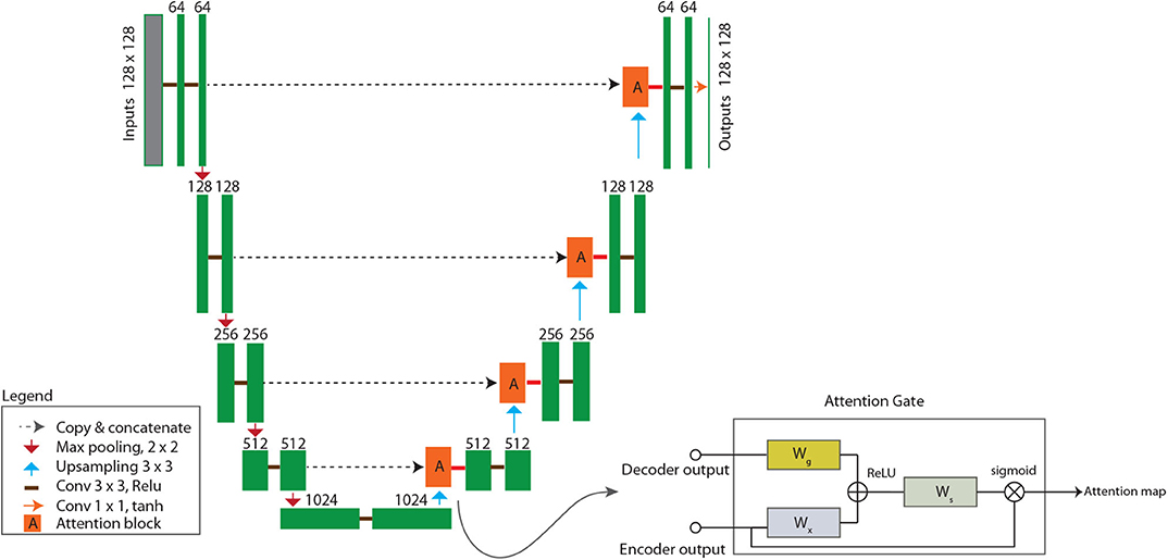
Figure 2. Model architecture of attention-based U-Net (AU-Net), which consists of a pair of encoder and decoder for end-to-end learning. Green blocks are convolutional blocks, for which the number of kernels used is labeled on top of each block. Red blocks are attention gate blocks, the design of which is shown in the callout on bottom right. Dashed arrow lines are skip connections. Most hidden convolutional layers use 3 × 3 kernels and the ReLU activation function, except in the attention block and in the output layer, where 1 × 1 kernels and tanh are used. Meanings of other symbols are explained in the legend shown at bottom left.

A key feature of the U-Net design is the skip connection, which is a combination of copy and concatenation operations to merge the fine-scale features from the downsampling step with the upsampled coarse-scale feature maps to better learn representations (dashed arrow lines in Figure 2) (Ronneberger et al., 2015). Mao et al. (2016) showed that the use of skip connections helps the training process to converge much faster and attain a higher-quality local optimum. So far, U-Net and its variants have been used in a large number of DL applications in geosciences (Sun, 2018; Arge et al., 2019; Karimpouli and Tahmasebi, 2019; Mo et al., 2019; Sun et al., 2019; Zhong et al., 2019; Zhu et al., 2019).

In CNN design, the size of the receptive field (e.g., kernel dimensions) directly affects the learning performance. If a single, fixed-size kernel is used to scan the inputs, global information may be missed, especially when the resolution of the input image is high. In the literature, several methods have been proposed to circumvent the issue. The skip connection used in U-Net is one example. As another example, Ren et al. (2016) proposed a multiscale CNN model consisting of a pair of coarse-scale and fine-scale autoencoders, the former uses a 11 × 11 kernel, while the latter uses a 7 × 7 kernel; the output of the coarse network is fed to the fine network as additional information to refine the coarse prediction with details. In recent years, self-attention has emerged as yet another alternative for capturing multiscale contexts in an image.

Simply speaking, attention refers to the biological capability of certain animals, including humans, to direct their gaze rapidly toward objects of interest in a visual environment, transforming the understanding of a visual scene into a series of computationally less demanding, localized visual analysis problems (Itti and Koch, 2001). Significant interests exist in computational neuroscience to replicate such capability in pattern recognition algorithms. In machine translation (natural language processing), for example, self-attention has been proposed as a mechanism for relating different positions of a single sequence in order to compute a representation of the sequence (Vaswani et al., 2017). In image processing, attention has been used to model the image as a sequence of regions, allowing for better capturing of large-scale features while producing sharper local details, thus leading to improved performance in object tracking, object detection, and image caption generation applications (Xu et al., 2015; Oktay et al., 2018; Bello et al., 2019; Hou et al., 2019). For this study, we hypothesize that the same attention mechanism that helps to capture multiscale spatial and temporal interactions may also be useful in learning the covariational patterns between high- and low-resolution precipitation products.

In general, attention-based algorithms work by suppressing the irrelevant background and enabling salient features to dynamically come to the forefront (Xu et al., 2015). We adopt the attention-gate module proposed by Oktay et al. (2018), which has the advantage of being compatible with the standard CNN models (e.g., U-Net) and can be added as an additional block without incurring significant computational overhead. As illustrated in Figure 2, the attention block is attached to the upsampling step of the U-Net (i.e., red blocks in Figure 2). For the l-th layer, the inputs to the attention block are outputs from the coarse-scale decoder (g^l) and that from the encoder (via the skip connection) (x^l). Inside the attention block, the inputs are passed through separate 1 × 1 convolutional layers, concatenated, and then passed through another 1 × 1 convolutional layer (with activation) to arrive at an attention map. In essence, the attention block may be regarded as a sub-network and its role is to suppress irrelevant features from the skip connections using information from the decoder. Mathematically, the series of attention gate operations may be described as (Oktay et al., 2018)

$\begin{array}{ll}{\text{q}}^l={\text{W}}_s\otimes \left({\sigma }_1\left({\text{W}}_x\otimes {\text{x}}^l+{\text{b}}_x+{\text{W}}_g\otimes {\text{g}}^l+{\text{b}}_g\right)\right)+b_s,& (3)\end{array}$

$\begin{array}{ll}{\alpha }^l={\sigma }_2\left({\text{q}}^l\left({\text{x}}^l,{\text{g}}^l;\Theta \right)\right),& (4)\end{array}$

where Θ = {W_x, W_g, b_g, b_x, b_s} represents a set of trainable weight matrices and bias terms, σ₁ is ReLU activation function, σ₂ is sigmoid activation function, α^l is the resulting attention map for weighting different regions in the input.

3.3. Network Training and Performance Metrics

Monthly data from 2001/01 to 2018/12 were divided into three parts, training (N_r = 168), validation (N_v = 24), and testing (N_t = 24). After preliminary analyses, four predictor groups were considered, including coarse-resolution satellite/reanalysis precipitation products (P), enhanced vegetation index (EVI), air temperature (T), elevation (DEM), slope, and aspect,

$\begin{array}{ll}{M}_1:P_{t-2:t},{EVI}_{t-1:t},DEM,Slope,Aspect,& (5)\end{array}$

$\begin{array}{ll}{M}_2:P_{t-2:t,}DEM,Slope,Aspect,& (6)\end{array}$

$\begin{array}{ll}{M}_3:P_{t-2:t,}DEM,& (7)\end{array}$

$\begin{array}{ll}{M}_4:P_{t-2:t},T_{t-2:t},& (8)\end{array}$

where the subscript t denotes the month index, and the target is PRISM data at month t. Models M₁ to M₃ include both static and dynamic variables, while M₄ only includes coarse-resolution dynamic variables. All AU-Net models are developed at the 128 × 128 grid resolution, which is about 2.6 km/pixel for the current problem. The lags for the dynamic variables are chosen based on preliminary analyses. Higher-resolution grids are tested as part of the sensitivity study. Before training, all inputs are resampled to the same grid resolution through bilinear interpolation, and then normalized before passing to the DL model for training.

All models were developed in the PyTorch (v1.1) machine learning framework. The loss function used in training the AU-Net models is the mean square error (MSE) defined as

$\begin{array}{ll}\text{MSE}=\frac{1}{N_r}{\displaystyle \sum _{i=1}^{N_r}}\parallel {\text{y}}_i-{\widehat{\text{y}}}_i{\parallel }_2^2,& (9)\end{array}$

where y and $\widehat{\text{y}}$ represent the true precipitation data used for training and the predicted data, respectively. The ADAM solver (Kingma and Ba, 2014) was used to train the neural nets, with a learning rate α = 5 × 10⁻⁴, first moment decay rate β₁ = 0.5, and second moment decay rate β₂ = 0.999. During training and validation, the data samples were randomly shuffled to improve generalization. Training of the AU-Net was carried out on a dual-processor computing node equipped with 128Gb RAM and Nvidia 1080-TI GPU. A total of 100 epochs were used for each model and the batch size (i.e., number of samples used in each solver iteration) was set to 10. Early stopping was implemented by monitoring the validation loss to mitigate overfitting. Training time depends on the model size and grid resolution and generally takes about 15 min for each model at the 128 × 128 grid resolution.

Model performance evaluation includes comparison with both in situ gauge data and PRISM data for the testing period. For comparison with in situ data, three metrics are used, namely, the root mean square error (RMSE), bias, and correlation coefficient (CC),

$\begin{array}{ll}RMSE=\sqrt{\frac{1}{N_G}{\displaystyle \sum _{i=1}^{N_G}}{(y_{g,i}-{\widehat{y}}_i)}^2},& (10)\end{array}$

$\begin{array}{ll}BIAS=\frac{1}{N_G}\frac{{\displaystyle {\sum }_{N_G}}\left({\widehat{y}}_i-y_{g,i}\right)}{{\displaystyle {\sum }_{N_G}}\left(y_{g,i}\right)}\times 100,& (11)\end{array}$

$\begin{array}{ll}CC=\frac{1}{N_G{\sigma }_y{\sigma }_g}{\displaystyle \sum _i^{N_G}}(y_{g,i}-{\mu }_g)({\widehat{y}}_i-{\mu }_y),& (12)\end{array}$

where y_g and $\widehat{y}$ are measured and predicted data at a gauge location, N_G is the number of usable gauge data for a month, and μ and σ denote mean and standard deviation. If multiple gauges exist in a grid cell, we used the average of gauge values for that cell. Mean metric values were then obtained by averaging over all months in the testing period.

For image-to-image comparison, RMSE is calculated over all grid cells. In addition, the structural similarity index metric (SSIM) is calculated, which is a metric widely used in computer vision to measure similarity between two images (Wang et al., 2004). Specifically, for two sliding windows u and v operating separately on the testing and reference images (grayscale), SSIM is defined as

$\begin{array}{ll}\text{SSIM}(u,v)=\frac{(2{\mu }_u{\mu }_v+c_1)(2{\sigma }_{uv}+c_2)}{({\mu }_u^2+{\mu }_v^2+c_1)({\sigma }_u^2+{\sigma }_v^2+c_2)},& (13)\end{array}$

where μ and σ represent the mean and standard deviation of image patches falling in the sliding windows, and c₁ and c₂ are small constants introduced to avoid numerical instability (Wang et al., 2004). The global SSIM is obtained by averaging the patch SSIM values and is in the range [−1, 1], with higher values indicating better pattern matches. The sizes of sliding windows used are 11 × 11.

3.4. Residual Correction

Residual correction is commonly used in the final step of downscaling to fuse gauge observations (Haylock et al., 2006; Duan and Bastiaanssen, 2013; Chen et al., 2018). We experimented with both kriging and inverse distance weighting (IDW), and found that the latter gave better results. Thus, the IDW scheme was adopted to interpolate the residual errors between AU-Net results and gauge observations, e_i, to the entire grid, which were then added to the AU-Net estimates $\widehat{y}$. Specifically, the final estimate $\tilde{\text{y}}$ is obtained by

$\tilde{y}(\text{x})=\{\begin{array}{cc}{\displaystyle \widehat{y}(\text{x})+\left({\displaystyle {\sum }_{i=1}^{N_G}}{w}_i(\text{x})e_i\right)/\left({\displaystyle {\sum }_{i=1}^{N_G}}{w}_i(\text{x})\right),}\hfill & \text{if }d(\text{x},{\text{x}}_i)\ne 0\hfill \\ y_{g,i},\hfill & \text{if }d(\text{x},{\text{x}}_i)=0\hfill \end{array}$

where e_i = y_g,i − $\widehat{y}$_i is the residual calculated at a gauge location, d = ∥x−x_i∥ is the distance between a grid cell location x and a gauge location x_i, and the weight factor is $w_i=d^{-\beta }$. For this study, we set β = 2 based on error statistics calculated against PRISM data.

4. Results

For each coarse-resolution precipitation product (i.e., ERA5-Land, TRMM, and IMERG), the performance of four groups of predictors (M₁ − M₄) that are defined under section 3.3 were evaluated, leading to a total of 12 different AU-Net models. For brevity, IMERG will be simply referred to as GPM, and ERA5-Land as ERA5 in the following discussions.

As part of the exploratory analyses, the temporal correlations between PRISM and the coarse-resolution products at all 128 × 128 grid cell locations (i.e., after resampling via bilinear interpolation) were calculated and are shown in Figures 3A–C. The correlation maps of both TRMM and GPM exhibit similar spatial patterns, which tend to be higher in the eastern part and lower in the northwest high-elevation areas; all correlation values are above 0.8 (Note: despite the similarity, TRMM and IMERG processing are different in a number of ways, e.g., the Level-2 and Level-3 algorithms, the infrared data used for gap filling and replacement, as well as the spatiotemporal resolutions). In comparison, the correlation between ERA5 and PRISM is generally lower, except near the southwestern corner of the study area. Nevertheless, the large-scale spatial patterns of all three coarse-resolution products are similar, all exhibiting this diagonally oriented (southwest to northeast) stripe pattern.

FIGURE 3

Figure 3. Correlation maps between PRISM and (A) ERA, (B) TRMM, and (C) GPM over the entire study area. Correlation at each grid cell is calculated as the Pearson correlation coefficient between pairs of time series for that cell.

4.1. Performance of AU-Net Models

Figure 4 plots the training and validation errors vs. training epochs for all models. The ERA5 model group (Figure 4A) tends to have larger training and validation errors than TRMM (Figure 4B) and GPM (Figure 4C) groups. In each group, the M₄ AU-Net model tends to have slower training convergence rate and stronger oscillations than the rest of the models.

FIGURE 4

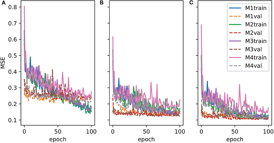
Figure 4. Convergence history of AU-Net training and validation: (A) ERA5, (B) TRMM, and (C) GPM.

Table 2 summarizes the mean performance metrics of all products and (uncorrected) AU-Net models against the gauge data for the test period 2017/01–2018/12. The target data, PRISM, has the smallest RMSE (3.59 cm) and highest CC (0.637) values. Among the three satellite/reanalysis products, TRMM and GPM have similar mean RMSE values (4.19 and 4.15 cm, respectively), which are all lower than that of the ERA5 (4.89 cm), but are more than 16% higher than that of the PRISM. The bias of TRMM (0.41) is lowest among all. GPM shows a slightly higher mean CC value (0.408), but is still about 35% lower than that of PRISM. Note that the CC values shown in Table 2 are lower than those seen previously in Figure 3. This is because the former quantifies the spatial correlation between gridded products and point measurements at gauge locations, while the latter measures CC between harmonized time series at each grid cell. Also rain gauges are subject to various errors as mentioned in the Introduction, and point-scale gauge measurements may deviate significantly from areal precipitation (Tang et al., 2018a).

TABLE 2

Table 2. Summary of gauge comparison metrics on testing data (2017/01–2018/12) for three precipitation products, ERA5, TRMM, and GPM, and AU-Net models (best performing member in each category is highlighted).

At the gauge level, Table 2 suggests that the AU-Net models in the ERA5 group show similar mean RMSE and CC, but the bias is reduced significantly compared to the original ERA5. The AU-Net models for TRMM show slightly worse RMSE than the original TRMM, and slightly better CC, but the bias is also larger. The same is true for GPM AU-Net models. All the metrics are summarized in Figures 5A–C in separate Taylor diagrams (Taylor, 2001), which help to visualize model performance in terms of CC, standard deviation (SD), and RMSE relative to the reference gauge observations. The Taylor diagrams suggest that all gridded precipitation products underestimate the data spread as seen in the gauge data, which is due to the harmonization process behind the gridded products. ERA5 has the greatest SD, while TRMM and GPM have similar SD values. The AU-Net models for different data groups are mostly clustered together, although the M₁ models seem to do better than others.

FIGURE 5

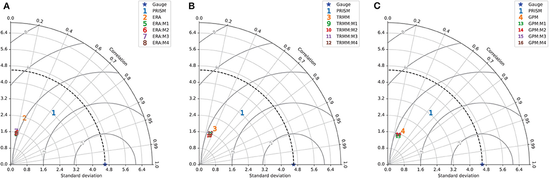
Figure 5. Taylor diagrams summarizing statistics of all gridded rainfall products and uncorrected AU-Net models, against the gauge data and PRISM data for test period (2017/01–2018/12): (A) ERA, (B) TRMM, and (C) GPM. The blue star on the horizontal axes corresponds to the gauge dataset result.

In Supplementary Figures 1–3, boxplots of the monthly values of MSE, bias, and CC for each AU-Net model are provided. In general, the boxplots support the aforementioned observations. Moreover, they also suggest that the range of model performance metrics depends on the quality of the coarse-resolution inputs. For example, models trained using TRMM and GPM, both are already gauge corrected, generally exhibit smaller variations in metric values than the models trained using ERA5 do.

Overall, on the basis of rain gauge data comparison, the best performers are scattered among predictor groups M₁–M₃ for the three products considered. The M₄ group seems to underperform compared to the other three predictor groups, due to its use of only coarse-scale information.

At the grid-level, Figures 6–8 show the monthly time series of performance metrics for each product. The top panel of each figure compares the spatially averaged precipitation calculated on PRISM and the respective data product. In general, results suggest that the model performance is sensitive to the amount of precipitation, as well as to antecedent conditions of dynamic variables (i.e., P, T, and EVI). The models tend to outperform the baseline coarse-resolution product in dry months than in wet months. For ERA5, models M₁ and M₃ improve over ERA5 (as measured in SSIM) in the mid part of the test period, ranging from 2017/03 to 2018/06. Most ERA5 models, however, underperform the original ERA5 data during two extreme wet events, one in 2017/08 when Hurricane Harvey made landfall and the other during the record-breaking wet period 2018/08–2018/09. This may be attributed to the extremity of the events and the lack of predictability at the monthly scale. In the case of TRMM and GPM models, the metrics time series are less oscillatory—all models tend to have very similar RMSE values, and the model SSIM values are better than the TRMM and GPM during the dry period in the middle of the test period. Compared to ERA, the metrics of TRMM and GPM model stay close to the original data products even during the two extreme events.

FIGURE 6

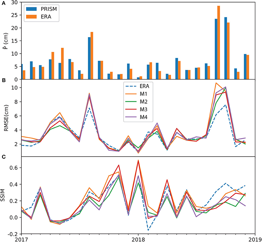
Figure 6. Time series of ERA metrics over the test period (2017/01–2018/12): (A) monthly averaged PRISM and ERA data; (B) mean grid averaged RMSE; and (C) SSIM. All subplots share the same x axis.

FIGURE 7

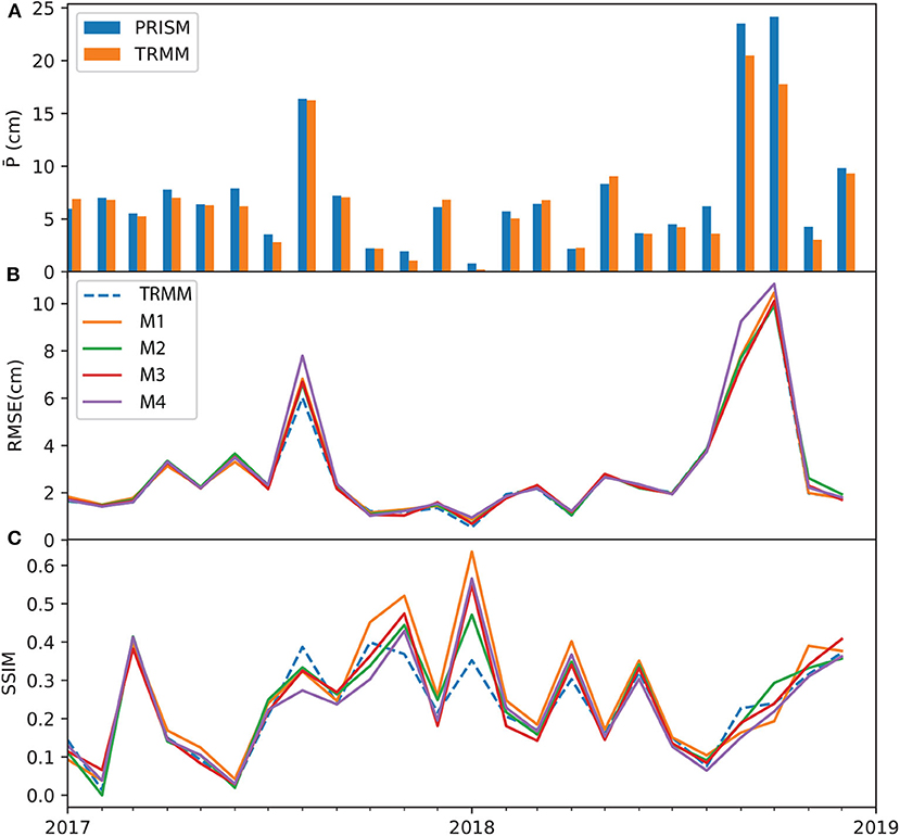
Figure 7. Time series of TRMM metrics over the test period: (A) monthly averaged PRISM and TRMM data; (B) mean grid averaged RMSE; and (C) SSIM. All subplots share the same x axis.

FIGURE 8

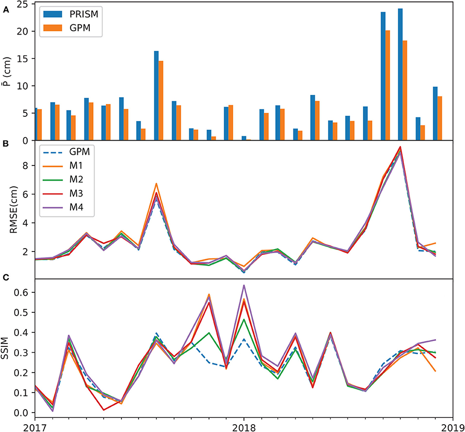
Figure 8. Time series of GPM metrics over the test period: (A) monthly averaged PRISM and GPM data; (B) mean grid averaged RMSE; and (C) SSIM. All subplots share the same x axis.

To give examples of learned patterns, in Figure 9 we plot the AU-Net results (left three columns), together with the original coarse-resolution data (top row) and the fine-resolution PRISM and Stage-IV datasets (the rightmost column) for 2017/01, which was a relatively wet month. The SSIM between each image and PRISM is shown on top of each subplot. PRISM and Stage-IV have very similar spatial patterns. Compared to the PRISM and Stage-IV data, ERA5 (upper-left) did not capture the higher rainfall zone near the eastern side, while both TRMM and GPM were able to capture the same zone in a large-scale sense. The AU-Net models that include static information (i.e., M₁–M₃) introduce more fine-scale features in the results, such as near the southwestern corner of the domain and inside the wetter zone; however, the improvements over the original products are rather limited in terms of SSIM. Only the M₂ model under the GPM group predicts the location of the high-precipitation relatively accurately. The M₄ models, which only use coarse-resolution information, yield more smooth features than the other models do.

FIGURE 9

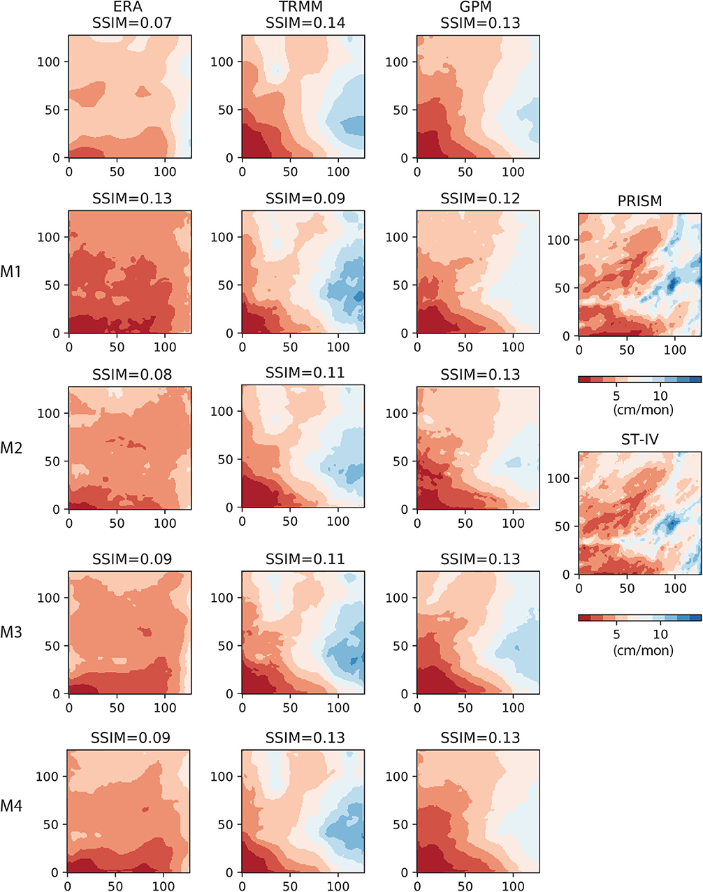
Figure 9. AU-Net results on 2017/01 data (128 × 128 grid). Left column (from top to bottom) ERA5 and the corresponding M₁ − M₄ AU-Net models; 2nd column: TRMM and the corresponding AU-Net models; 3rd column: GPM and the corresponding AU-Net models; rightmost column: PRISM and the reference Stage-IV data for the same month. All subplots are scaled to the same color range.

As another example, we compare the AU-Net results for the month 2018/01, which was a relatively dry month. Figure 10 shows that all three coarse-resolution products are able to delineate the large low-precipitation zone near the northwestern corner. Under the ERA group, the M₁ model gives the best pattern match (SSIM = 0.69), while in the cases of TRMM and GPM, M₁ (SSIM = 0.63) and M₄ (SSIM = 0.67) give the best pattern match, respectively. In this case, even the M₄ model, which only uses dynamic variables, is able to infill some fine-scale features.

FIGURE 10

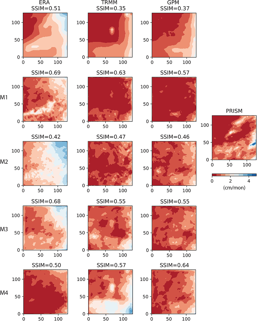
Figure 10. AU-Net results on 2018/01 data (128 × 128 grid). Left column (from top to bottom): ERA5 and the corresponding M₁ − M₄ AU-Net models; 2nd column: TRMM and the corresponding AU-Net models; 3rd column: GPM and the corresponding AU-Net models; rightmost column: PRISM data for the same month.

Results in Figures 9, 10 highlight the promises, as well as challenges, in extracting and learning the fine-scale features in precipitation data for this low-predictability study area. The use of antecedent conditions and auxiliary static information helped to improve the baseline coarse-resolution products in some cases, but deteriorated the baseline in other cases. In particular, we note that static information tends to be more useful under dry conditions, while autocorrelation in precipitation itself seems to play a major role in predictability. No predictor group consistently performed better than the others. The inherent high variability of precipitation in space and time, especially in topographically complex regions, makes the pattern-based downscaling challenging, without further correction using in situ data.

4.2. Corrected AU-Net Models

The AU-Net models were corrected by first calculating the error residual between model and gauge data, and then interpolating to the grid using the IDW scheme described under this section. Figure 11 shows the gauge-corrected AU-Net results on the 2017/01 data used in Figure 9. Similarly, Figure 12 shows the gauge corrected results for 2018/01 data. Results suggest that gauge correction significantly improved the pattern match for all AU-Net models, leading to convergence in model patterns among all models. In the case of 2017/01, gauge correction actually introduced more fine-scale features than that are present in the PRISM image. This may be caused by the difference in point measurement set used, and also in the gauge data interpolation algorithm. In the case of 2018/01, gauge correction almost resulted in identical patterns to the PRISM image. The dominating effect of gauge correction observed here is not surprising, given the large number of gauges available for the study area (361 in 2017/01 and 459 in 2018/01). RMSE of the gauge-corrected AU-Net models (not reported here) is also significantly reduced, compared to the uncorrected results.

FIGURE 11

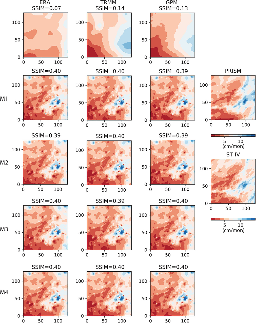
Figure 11. Results of gauge correction using inverse distance weighting on 2017/01 data. Left column (from top to bottom) ERA5 and the corresponding M₁ − M₄ AU-Net models; 2nd column: TRMM and the corresponding AU-Net models; 3rd column: GPM and the corresponding AU-Net models; rightmost column: reference PRISM and Stage-IV data for the same month.

FIGURE 12

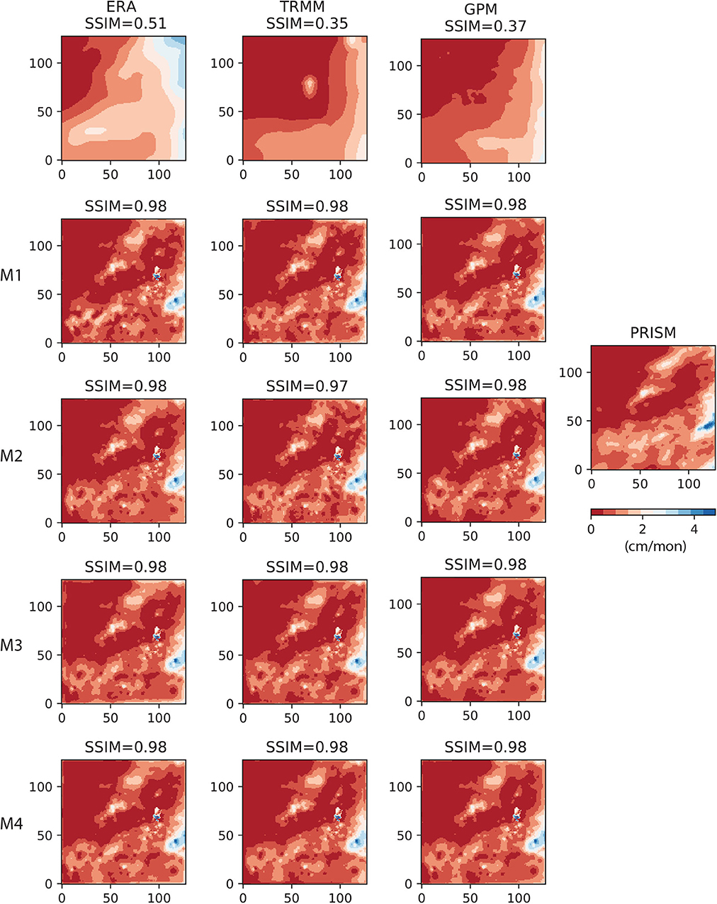
Figure 12. Results of gauge correction on 2018/01 data. Left column (from top to bottom) ERA5 and the corresponding M₁ − M₄ AU-Net models; 2nd column: TRMM and the corresponding AU-Net models; 3rd column: GPM and the corresponding AU-Net models; rightmost column: reference PRISM data for the same month.

4.3. Effect of Attention Mechanism

A main motivation of this work to explore the use of attention mechanism for multiscale pattern extraction. To demonstrate the effect of attention mechanism, we train the classic U-Net models using the same model structures, but with the attention block removed (see Figure 2). The kernel size used in the U-Net is 4 × 4 and stride size is 2. As mentioned before, attention mechanism helps to capture the large-scale patterns while producing sharper local details. Figure 13 shows the result for the same 2017/01 data, as shown earlier in Figure 9. An immediate observation from Figure 9 is that all images produced by the U-Net are more blurry than those generated by the AU-Net models. The SSIM values are also smaller than their counterparts in AU-Nets.

FIGURE 13

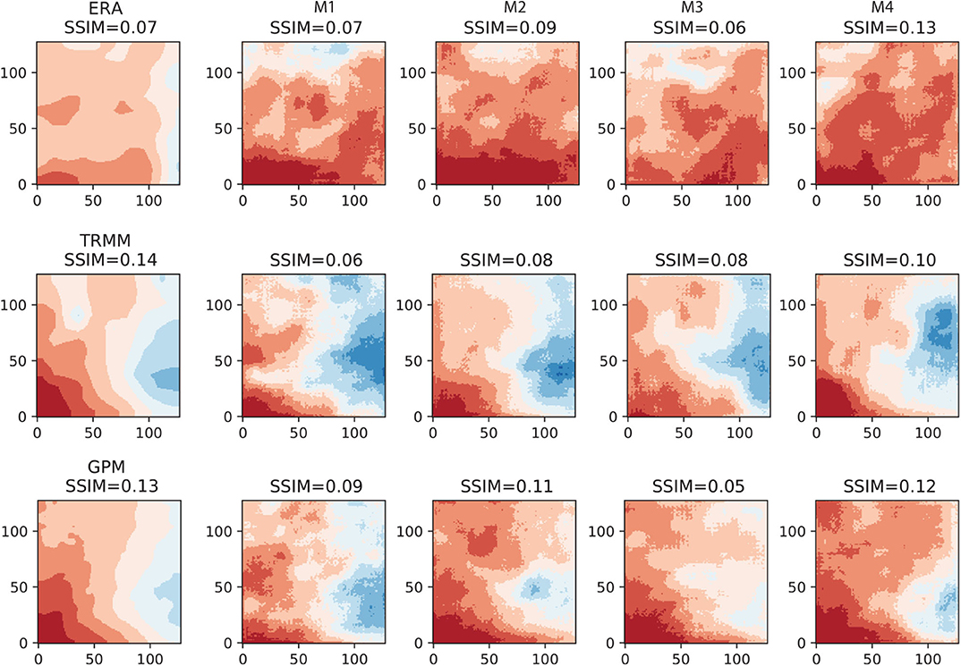
Figure 13. Results of U-Net models for 2017/01. Top row: ERA5 results; mid-row: TRMM results; and bottom row: GPM results.

5. Discussion

In this work, the feasibility of using AU-Net to downscale precipitation data was investigated over Central Texas, U.S., on three coarse-resolution satellite/reanalysis products. Climate in the region ranges from semi-arid in the west to subtropical in the east. The climate and hilly terrain of the region lead to strong spatial and temporal variations in precipitation patterns, making downscaling for the study area at the monthly level especially challenging. The AU-Net models, which can extract features at multiple scales, are used to learn the mappings between coarse- and fine-resolution products.

At the regionally aggregated scale, all three coarse-resolution products (baseline) are shown to have relatively strong temporal correlation with the fine-resolution PRISM product (>0.7) at the monthly level. The question is whether this correlation can be propagated down to the grid level. A main finding of this study is that the efficacy of downscaling and thus, model improvement, depends on the precipitation amount and information content embedded in antecedent conditions and auxiliary variables, as well as the quality of the original product. Under drier conditions, the precipitation patterns are more contiguous and are easier for the AU-Net models to learn. In addition, the static information tends to be more useful under drier conditions. On the other hand, in wet months the precipitation patterns become spatially heterogeneous and are more difficult to downscale without additional constraints. This observation is largely in agreement with the previous studies that show systematic errors in precipitation products are proportional to precipitation rates, which is higher for higher rates (e.g., AghaKouchak et al., 2012).

The fine-resolution auxiliary variables considered in this study only include EVI and DEM. EVI may be less reliable as a predictor at the monthly level (Duan and Bastiaanssen, 2013), even with added lags. Thus, future effort should focus on experimenting with alternative fine-resolution remotely sensed information, which is especially valuable when high-density rain gauge networks are not available.

Performance of DL models may depend on grid resolution. Higher grid resolution models, however, also increase training time significantly. In this work, we mainly experiment with 128 × 128 grids. As a sensitivity analysis, we also trained the same AU-Net models on 256 × 256 grids. The average training time is about 30 min on the same computing node. The results, which are compared in Supplementary Material S2, indicate that finer resolution tends to improve error metrics across all groups. The relative performance between models and the original products remains about the same.

The monthly scale considered in this work limits the number of data samples available for training which, in turn, may also affect the network performance. Future work will examine daily scales. At last, in this work we assume that the ground truth is PRISM, which itself may be subject to uncertainties present in the rain gauge data.

6. Summary

High-resolution precipitation data is needed in a large number of hydrological planning and emergency management activities. Currently, a number of coarse-resolution remotely sensed products are produced on operational basis. To maximize the societal benefits of these products, some type of downscaling is necessary, which is a highly ill-posed inverse problem. This work investigates the feasibility of deep-learning-based downscaling approaches by considering different combinations of static and dynamic variables as predictors. The state-of-the-art, end-to-end deep learning (DL) framework adopted in this study allows for stacking of multi-source and multi-resolution inputs. In addition, we explore a new attention mechanism for learning multiscale features (i.e., AU-Net). The efficacy of the AU-Net is demonstrated over Central Texas, U.S., for downscaling three coarse-resolution precipitation products, namely, ERA, TRMM, and IMERG data. Results suggest that the trained AU-Net models achieve different degrees of success in downscaling the coarse-resolution products. In general, the model performance depends on the precipitation rate, and the performance is better under nominal and dry conditions than in extremely wet conditions.

Although we mainly demonstrate an attention-based, DL framework for a low-predictability study area in the U.S., the problem setup is general and the approach can be applied to other regions and at different spatial and temporal resolutions.

Data Availability Statement

The raw data supporting the conclusions of this article will be made available by the authors, without undue reservation, to any qualified researcher.

Author Contributions

AS and GT conceived the original idea, discussed the results, and contributed to the final manuscript. AS developed the machine learning code and performed the computations. All authors contributed to the article and approved the submitted version.

Funding

AS was partly supported by Planet Texas 2050 Initiative funded by VP for Research Office at the University of Texas at Austin.

Conflict of Interest

The authors declare that the research was conducted in the absence of any commercial or financial relationships that could be construed as a potential conflict of interest.

Acknowledgments

The authors were grateful to the handling editor and the reviewers for their constructive comments.

Supplementary Material

The Supplementary Material for this article can be found online at: https://www.frontiersin.org/articles/10.3389/frwa.2020.536743/full#supplementary-material

References

AghaKouchak, A., Mehran, A., Norouzi, H., and Behrangi, A. (2012). Systematic and random error components in satellite precipitation data sets. Geophys. Res. Lett. 39, 1–4. doi: 10.1029/2012GL051592

CrossRef Full Text | Google Scholar

Arge, L., Grønlund, A., Svendsen, S. C., and Tranberg, J. (2019). Learning to find hydrological corrections. arXiv[Preprint].arXiv:1909.07685. doi: 10.1145/3347146.3359095

CrossRef Full Text | Google Scholar

Austin Statesman (2019). Available online at: https://www.statesman.com/news/20190418/austin-region-fastest-growing-large-metro-in-nation-8-years-running-data-shows (accessed October 15, 2019).

Barnes, R. (2018). RichDEM: High-Performance Terrain Analysis. Technical Report. PeerJ Preprints.

Google Scholar

Beck, H. E., Pan, M., Roy, T., Weedon, G. P., Pappenberger, F., Van Dijk, A. I., et al. (2019). Daily evaluation of 26 precipitation datasets using stage-iv gauge-radar data for the conus. Hydrol. Earth Syst. Sci. 23, 207–224. doi: 10.5194/hess-23-207-2019

CrossRef Full Text | Google Scholar

Beck, H. E., Van Dijk, A. I., Levizzani, V., Schellekens, J., Gonzalez Miralles, D., Martens, B., et al. (2017). Mswep: 3-hourly 0.25 global gridded precipitation (1979–2015) by merging gauge, satellite, and reanalysis data. Hydrol. Earth Syst. Sci. 21, 589–615. doi: 10.5194/hess-21-589-2017

CrossRef Full Text | Google Scholar

Becker, A., Finger, P., Meyer-Christoffer, A., Rudolf, B., Schamm, K., Schneider, U., et al. (2013). A description of the global land-surface precipitation data products of the global precipitation climatology centre with sample applications including centennial (trend) analysis from 1901–present. Earth Syst. Sci. Data 5, 71–99. doi: 10.5194/essd-5-71-2013

CrossRef Full Text | Google Scholar

Bello, I., Zoph, B., Vaswani, A., Shlens, J., and Le, Q. V. (2019). Attention augmented convolutional networks. arXiv[Preprint].arXiv:1904.09925. doi: 10.1109/ICCV.2019.00338

CrossRef Full Text | Google Scholar

Bolvin, D., and Huffman, G. (2015). Transition of 3B42/3B43 Research Product From Monthly to Climatological Calibration/Adjustment. NASA Precipitation Measurement Missions Document. Washington, DC: NASA.

Chen, Y., Huang, J., Sheng, S., Mansaray, L. R., Liu, Z., Wu, H., et al. (2018). A new downscaling-integration framework for high-resolution monthly precipitation estimates: combining rain gauge observations, satellite-derived precipitation data and geographical ancillary data. Rem. Sens. Environ. 214, 154–172. doi: 10.1016/j.rse.2018.05.021

CrossRef Full Text | Google Scholar

Daly, C., Taylor, G., and Gibson, W. (1997). “The PRISM approach to mapping precipitation and temperature,” in Proceedings of 10th AMS Conference on Applied Climatology, Oct 20–23, Reno, NV. p. 1–4.

Dee, D. P., Uppala, S., Simmons, A., Berrisford, P., Poli, P., Kobayashi, S., et al. (2011). The era-interim reanalysis: configuration and performance of the data assimilation system. Q. J. R. Meteorol. Soc. 137, 553–597. doi: 10.1002/qj.828

CrossRef Full Text | Google Scholar

Duan, Z., and Bastiaanssen, W. (2013). First results from version 7 TRMM 3B43 precipitation product in combination with a new downscaling–calibration procedure. Rem. Sens. Environ. 131, 1–13. doi: 10.1016/j.rse.2012.12.002

CrossRef Full Text | Google Scholar

Goodfellow, I., Bengio, Y., Courville, A., and Bengio, Y. (2016). Deep learning. Cambridge, MA: MIT Press.

Google Scholar

Haylock, M. R., Cawley, G. C., Harpham, C., Wilby, R. L., and Goodess, C. M. (2006). Downscaling heavy precipitation over the united kingdom: a comparison of dynamical and statistical methods and their future scenarios. Int. J. Climatol. 26, 1397–1415. doi: 10.1002/joc.1318

CrossRef Full Text | Google Scholar

He, X., Chaney, N. W., Schleiss, M., and Sheffield, J. (2016). Spatial downscaling of precipitation using adaptable random forests. Water Resour. Res. 52, 8217–8237. doi: 10.1002/2016WR019034

CrossRef Full Text | Google Scholar

Hennermann, K., and Berrisford, P. (2017). Era5 Data Documentation. Copernicus Knowledge Base. Available online at: https://confluence.ecmwf.int/display/CKB/ERA5 (accessed November 09, 2020).

Hirschboeck, K. (1987). “Catastrophic flooding and atmospheric circulation anomalies (USA),” in Catastrophic Flooding. eds. L. Mayer and D. B. Nash (Boston: Allen & Unwin), p. 23–56.

Google Scholar

Hong, Y., Adler, R. F., Negri, A., and Huffman, G. J. (2007). Flood and landslide applications of near real-time satellite rainfall products. Nat. Hazards 43, 285–294. doi: 10.1007/s11069-006-9106-x

CrossRef Full Text | Google Scholar

Hou, A. Y., Kakar, R. K., Neeck, S., Azarbarzin, A. A., Kummerow, C. D., Kojima, M., et al. (2014). The global precipitation measurement mission. Bull. Am. Meteorol. Soc. 95, 701–722. doi: 10.1175/BAMS-D-13-00164.1

CrossRef Full Text | Google Scholar

Hou, Y., Ma, Z., Liu, C., and Loy, C. C. (2019). Learning lightweight lane detection CNNs by self attention distillation. arXiv[Preprint].arXiv:1908.00821. doi: 10.1109/ICCV.2019.00110

CrossRef Full Text | Google Scholar

Huffman, G. J., Adler, R. F., Bolvin, D. T., and Nelkin, E. J. (2010). “The TRMM multi-satellite precipitation analysis (TMPA),” in Satellite Rainfall Applications for Surface Hydrology. eds. M. Gebremichael and F. Hossain (Dordrecht: Springer). doi: 10.1007/978-90-481-2915-7_1

CrossRef Full Text | Google Scholar

Huffman, G. J., Bolvin, D. T., Braithwaite, D., Hsu, K., Joyce, R., Xie, P., et al. (2015). NASA global precipitation measurement (GPM) integrated multi-satellite retrievals for GPM (IMERG). Algorithm Theor. Basis Doc. 4:30. Available online at: https://docserver.gesdisc.eosdis.nasa.gov/public/project/GPM/IMERG_ATBD_V06.pdf (accessed November 09, 2020).

Google Scholar

Huffman, G. J., Bolvin, D. T., Nelkin, E. J., Wolff, D. B., Adler, R. F., Gu, G., et al. (2007). The TRMM multisatellite precipitation analysis (TMPA): quasi-global, multiyear, combined-sensor precipitation estimates at fine scales. J. Hydrometeorol. 8, 38–55. doi: 10.1175/JHM560.1

CrossRef Full Text | Google Scholar

Itti, L., and Koch, C. (2001). Computational modelling of visual attention. Nat. Rev. Neurosci. 2:194. doi: 10.1038/35058500

CrossRef Full Text | Google Scholar

Jakob Themeßl, M., Gobiet, A., and Leuprecht, A. (2011). Empirical-statistical downscaling and error correction of daily precipitation from regional climate models. Int. J. Climatol. 31, 1530–1544. doi: 10.1002/joc.2168

CrossRef Full Text | Google Scholar

Jean, N., Burke, M., Xie, M., Davis, W. M., Lobell, D. B., and Ermon, S. (2016). Combining satellite imagery and machine learning to predict poverty. Science 353, 790–794. doi: 10.1126/science.aaf7894

PubMed Abstract | CrossRef Full Text | Google Scholar

Jia, S., Zhu, W., Lű, A., and Yan, T. (2011). A statistical spatial downscaling algorithm of TRMM precipitation based on NDVI and DEM in the Qaidam basin of China. Rem. Sens. Environ. 115, 3069–3079. doi: 10.1016/j.rse.2011.06.009

CrossRef Full Text | Google Scholar

Karimpouli, S., and Tahmasebi, P. (2019). Segmentation of digital rock images using deep convolutional autoencoder networks. Comput. Geosci. 126, 142–150. doi: 10.1016/j.cageo.2019.02.003

CrossRef Full Text | Google Scholar

Kidd, C., Becker, A., Huffman, G. J., Muller, C. L., Joe, P., Skofronick-Jackson, G., et al. (2017). So, how much of the earth's surface is covered by rain gaugee? Bull. Am. Meteorol. Soc. 98, 69–78. doi: 10.1175/BAMS-D-14-00283.1

PubMed Abstract | CrossRef Full Text | Google Scholar

Kim, S., Hong, S., Joh, M., and Song, S. K. (2017). Deeprain: convLSTM network for precipitation prediction using multichannel radar data. arXiv 1711.02316.

Google Scholar

Kingma, D. P., and Ba, J. (2014). Adam: a method for stochastic optimization. arXiv[Preprint].arXiv:1412.6980.

Google Scholar

Kistler, R., Kalnay, E., Collins, W., Saha, S., White, G., Woollen, J., et al. (2001). The NCEP–NCAR 50-year reanalysis: monthly means CD-ROM and documentation. Bull. Am. Meteorol. Soc. 82, 247–268. doi: 10.1175/1520-0477(2001)082<0247:TNNYRM>2.3.CO;2

CrossRef Full Text | Google Scholar

Li, H., Sheffield, J., and Wood, E. F. (2010). Bias correction of monthly precipitation and temperature fields from intergovernmental panel on climate change AR4 models using equidistant quantile matching. J. Geophys. Res. Atmos. 115, 1–20. doi: 10.1029/2009JD012882

CrossRef Full Text | Google Scholar

Lin, Y., and Mitchell, K. E. (2005). “1.2 the NCEP stage II/IV hourly precipitation analyses: development and applications,” in 19th Conference on Hydrology (San Diego, CA: American Meteorological Society; Citeseer).

Google Scholar

Long, D., Scanlon, B. R., Longuevergne, L., Sun, A. Y., Fernando, D. N., and Save, H. (2013). Grace satellite monitoring of large depletion in water storage in response to the 2011 drought in Texas. Geophys. Res. Lett. 40, 3395–3401. doi: 10.1002/grl.50655

CrossRef Full Text | Google Scholar

López López, P., Immerzeel, W. W., Rodríguez Sandoval, E. A., Sterk, G., and Schellekens, J. (2018). Spatial downscaling of satellite-based precipitation and its impact on discharge simulations in the Magdalena river basin in Colombia. Front. Earth Sci. 6:68. doi: 10.3389/feart.2018.00068

CrossRef Full Text | Google Scholar

Lowrey, M. R. K., and Yang, Z. L. (2008). Assessing the capability of a regional-scale weather model to simulate extreme precipitation patterns and flooding in central Texas. Weather Forecast. 23, 1102–1126. doi: 10.1175/2008WAF2006082.1

CrossRef Full Text | Google Scholar

Ma, Y., Wu, H., Wang, L., Huang, B., Ranjan, R., Zomaya, A., et al. (2015). Remote sensing big data computing: challenges and opportunities. Fut. Gen. Comput. Syst. 51, 47–60. doi: 10.1016/j.future.2014.10.029

CrossRef Full Text | Google Scholar

Mace, R. E., Chowdhury, A. H., Anaya, R., and Way, S. C. (2000). Groundwater availability of the Trinity Aquifer, Hill Country Area, Texas: numerical simulations through 2050. Texas Water Dev. Board Rep. 353:117. Available online at: https://www.twdb.texas.gov/publications/reports/numbered_reports/doc/R353/Report353.pdf (accessed November 09, 2020).

Google Scholar

Mao, X., Shen, C., and Yang, Y. B. (2016). “Image restoration using very deep convolutional encoder-decoder networks with symmetric skip connections,” in Proceedings of the 30th International Conference on Neural Information Processing Systems, Barcelona. p. 2810–2818.

Google Scholar

Maraun, D., Wetterhall, F., Ireson, A., Chandler, R., Kendon, E., Widmann, M., et al. (2010). Precipitation downscaling under climate change: recent developments to bridge the gap between dynamical models and the end user. Rev. Geophys. 48, 1–34. doi: 10.1029/2009RG000314

CrossRef Full Text | Google Scholar

Miao, Q., Pan, B., Wang, H., Hsu, K., and Sorooshian, S. (2019). Improving monsoon precipitation prediction using combined convolutional and long short term memory neural network. Water 11:977. doi: 10.3390/w11050977

CrossRef Full Text | Google Scholar

Mo, S., Zhu, Y., Zabaras, N., Shi, X., and Wu, J. (2019). Deep convolutional encoder-decoder networks for uncertainty quantification of dynamic multiphase flow in heterogeneous media. Water Resour. Res. 55, 703–728. doi: 10.1029/2018WR023528

CrossRef Full Text | Google Scholar

Nielsen-Gammon, J. W., Zhang, F., Odins, A. M., and Myoung, B. (2005). Extreme rainfall in Texas: patterns and predictability. Phys. Geogr. 26, 340–364. doi: 10.2747/0272-3646.26.5.340

CrossRef Full Text | Google Scholar

Oktay, O., Schlemper, J., Folgoc, L. L., Lee, M., Heinrich, M., Misawa, K., et al. (2018). Attention U-net: learning where to look for the pancreas. arXiv[Preprint].arXiv:1804.03999.

Google Scholar

Omranian, E., and Sharif, H. O. (2018). Evaluation of the global precipitation measurement (GPM) satellite rainfall products over the lower Colorado river basin, Texas. J. Am. Water Resour. Assoc. 54, 882–898. doi: 10.1111/1752-1688.12610

CrossRef Full Text | Google Scholar

Pan, B., Hsu, K., AghaKouchak, A., and Sorooshian, S. (2019). Improving precipitation estimation using convolutional neural network. Water Resour. Res. 55, 2301–2321. doi: 10.1029/2018WR024090

CrossRef Full Text | Google Scholar

Pan, S. J., and Yang, Q. (2009). A survey on transfer learning. IEEE Trans. Knowl. Data Eng. 22, 1345–1359. doi: 10.1109/TKDE.2009.191

CrossRef Full Text | Google Scholar

Quiroz, R., Yarlequé, C., Posadas, A., Mares, V., and Immerzeel, W. W. (2011). Improving daily rainfall estimation from NDVI using a wavelet transform. Environ. Model. Softw. 26, 201–209. doi: 10.1016/j.envsoft.2010.07.006

CrossRef Full Text | Google Scholar

Ren, W., Liu, S., Zhang, H., Pan, J., Cao, X., and Yang, M. H. (2016). “Single image dehazing via multi-scale convolutional neural networks,” in European Conference on Computer Vision Oct 8–16 (Amsterdam: Springer), 154–169.

Google Scholar

Rienecker, M. M., Suarez, M. J., Gelaro, R., Todling, R., Bacmeister, J., Liu, E., et al. (2011). MERRA: NASA's modern-era retrospective analysis for research and applications. J. Clim. 24, 3624–3648. doi: 10.1175/JCLI-D-11-00015.1

CrossRef Full Text | Google Scholar

Ronneberger, O., Fischer, P., and Brox, T. (2015). “U-net: convolutional networks for biomedical image segmentation,” in International Conference on Medical Image Computing and Computer-Assisted Intervention (Munich: Springer), 234–241.

Google Scholar

Saha, S., Moorthi, S., Pan, H. L., Wu, X., Wang, J., Nadiga, S., et al. (2010). The NCEP climate forecast system reanalysis. Bull. Am. Meteorol. Soc. 91, 1015–1058. doi: 10.1175/2010BAMS3001.1

CrossRef Full Text | Google Scholar

Scanlon, B. R., Zhang, Z., Save, H., Sun, A. Y., Schmied, H. M., van Beek, L. P., et al. (2018). Global models underestimate large decadal declining and rising water storage trends relative to grace satellite data. Proc. Natl. Acad. Sci. U.S.A. 115, E1080–E1089. doi: 10.1073/pnas.1704665115

PubMed Abstract | CrossRef Full Text | Google Scholar

Schewe, J., Heinke, J., Gerten, D., Haddeland, I., Arnell, N. W., Clark, D. B., et al. (2014). Multimodel assessment of water scarcity under climate change. Proc. Natl. Acad. Sci. U.S.A. 111, 3245–3250. doi: 10.1073/pnas.1222460110

PubMed Abstract | CrossRef Full Text | Google Scholar

Seneviratne, S. I., Corti, T., Davin, E. L., Hirschi, M., Jaeger, E. B., Lehner, I., et al. (2010). Investigating soil moisture–climate interactions in a changing climate: a review. Earth Sci. Rev. 99, 125–161. doi: 10.1016/j.earscirev.2010.02.004

CrossRef Full Text | Google Scholar

Shen, Y., Zhao, P., Pan, Y., and Yu, J. (2014). A high spatiotemporal gauge-satellite merged precipitation analysis over china. J. Geophys. Res. Atmos. 119, 3063–3075. doi: 10.1002/2013JD020686

CrossRef Full Text | Google Scholar

Shi, X., Chen, Z., Wang, H., Yeung, D. Y., Wong, W. K., and Woo, W. C. (2015). “Convolutional LSTM network: a machine learning approach for precipitation nowcasting,” in Advances in Neural Information Processing Systems. eds. C. Cortes, N.D. Lawrence, D.D. Lee, M. Sugiyama and M. Garnett (Montreal) 802–810.

Google Scholar

Slade, R. M. Jr., and Patton, J. M. (2003). Major and Catastrophic Storms and Floods in Texas: 215 Major and 41 Catastrophic Events From 1953 to September 1, 2002. Technical Report. US Geological Survey.

Google Scholar

Sorooshian, S., AghaKouchak, A., Arkin, P., Eylander, J., Foufoula-Georgiou, E., Harmon, R., et al. (2011). Advanced concepts on remote sensing of precipitation at multiple scales. Bull. Am. Meteorol. Soc. 92, 1353–1357. doi: 10.1175/2011BAMS3158.1

CrossRef Full Text | Google Scholar

Sun, A. Y., Scanlon, B. R., Zhang, Z., Walling, D., Bhanja, S. N., Mukherjee, A., et al. (2019). Combining physically based modeling and deep learning for fusing grace satellite data: can we learn from mismatch? Water Resour. Res. 55, 1179–1195. doi: 10.1029/2018WR023333

CrossRef Full Text | Google Scholar

Sun, A. Y., and Scanlon, B. R. (2019). How can big data and machine learning benefit environment and water management: a survey of methods, applications, and future directions. Environ. Res. Lett. 14:073001. doi: 10.1088/1748-9326/ab1b7d

CrossRef Full Text | Google Scholar

Sun, A. Y., Wang, D., and Xu, X. (2014). Monthly streamflow forecasting using Gaussian process regression. J. Hydrol. 511, 72–81. doi: 10.1016/j.jhydrol.2014.01.023

CrossRef Full Text | Google Scholar

Sun, A. Y., Xia, Y., Caldwell, T. G., and Hao, Z. (2018). Patterns of precipitation and soil moisture extremes in Texas, US: a complex network analysis. Adv. Water Resour. 112, 203–213. doi: 10.1016/j.advwatres.2017.12.019

CrossRef Full Text | Google Scholar

Sun, A. Y. (2018). Discovering state-parameter mappings in subsurface models using generative adversarial networks. Geophys. Res. Lett. 45, 11–137. doi: 10.1029/2018GL080404

CrossRef Full Text | Google Scholar

Sun, Q., Miao, C., Duan, Q., Ashouri, H., Sorooshian, S., and Hsu, K. L. (2018). A review of global precipitation data sets: data sources, estimation, and intercomparisons. Rev. Geophys. 56, 79–107. doi: 10.1002/2017RG000574

CrossRef Full Text | Google Scholar

Tang, G., Behrangi, A., Long, D., Li, C., and Hong, Y. (2018a). Accounting for spatiotemporal errors of gauges: a critical step to evaluate gridded precipitation products. J. Hydrol. 559, 294–306. doi: 10.1016/j.jhydrol.2018.02.057

CrossRef Full Text | Google Scholar

Tang, G., Long, D., Behrangi, A., Wang, C., and Hong, Y. (2018b). Exploring deep neural networks to retrieve rain and snow in high latitudes using multisensor and reanalysis data. Water Resour. Res. 54, 8253–8278. doi: 10.1029/2018WR023830

CrossRef Full Text | Google Scholar

Tang, G., Zeng, Z., Long, D., Guo, X., Yong, B., Zhang, W., et al. (2016). Statistical and hydrological comparisons between TRMM and GPM level-3 products over a midlatitude basin: is day-1 IMERG a good successor for TMPA 3B42V7? J. Hydrometeorol. 17, 121–137. doi: 10.1175/JHM-D-15-0059.1

CrossRef Full Text | Google Scholar

Taylor, K. E. (2001). Summarizing multiple aspects of model performance in a single diagram. J. Geophys. Res. Atmos. 106, 7183–7192. doi: 10.1029/2000JD900719

CrossRef Full Text | Google Scholar

Trenberth, K. E., Smith, L., Qian, T., Dai, A., and Fasullo, J. (2007). Estimates of the global water budget and its annual cycle using observational and model data. J. Hydrometeorol. 8, 758–769. doi: 10.1175/JHM600.1

CrossRef Full Text | Google Scholar

Vandal, T., Kodra, E., Ganguly, S., Michaelis, A. R., Nemani, R. R., and Ganguly, A. R. (2018). “Generating high resolution climate change projections through single image super-resolution: an abridged version,” in IJCAI Jul 13–19 (Stockholm), 5389–5393.

Google Scholar

Vaswani, A., Shazeer, N., Parmar, N., Uszkoreit, J., Jones, L., Gomez, A. N., et al. (2017). “Attention is all you need,” in Advances in Neural Information Processing Systems. eds. I. Guyon, U. V. Luxburg, S. Bengio, H. Wallach, R. Fergus, S. Vishwanathan and R. Garnett (Long Beach, CA), 5998–6008.

Google Scholar

Vila, D. A., De Goncalves, L. G. G., Toll, D. L., and Rozante, J. R. (2009). Statistical evaluation of combined daily gauge observations and rainfall satellite estimates over continental south america. J. Hydrometeorol. 10, 533–543. doi: 10.1175/2008JHM1048.1

CrossRef Full Text | Google Scholar

Wang, Z., Bovik, A. C., Sheikh, H. R., and Simoncelli, E. P. (2004). Image quality assessment: from error visibility to structural similarity. IEEE Trans. Image Process. 13, 600–612. doi: 10.1109/TIP.2003.819861

PubMed Abstract | CrossRef Full Text | Google Scholar

Wood, E. F., Roundy, J. K., Troy, T. J., Van Beek, L., Bierkens, M. F., Blyth, E., et al. (2011). Hyperresolution global land surface modeling: meeting a grand challenge for monitoring earth's terrestrial water. Water Resour. Res. 47, 1–10. doi: 10.1029/2010WR010090

CrossRef Full Text | Google Scholar

Xu, K., Ba, J., Kiros, R., Cho, K., Courville, A., Salakhudinov, R., et al. (2015). “Show, attend and tell: neural image caption generation with visual attention,” in: International Conference on Machine Learning Jul 6–15. Lile. p. 2048–2057.

Google Scholar

Yang, Z., Hsu, K., Sorooshian, S., Xu, X., Braithwaite, D., and Verbist, K. M. (2016). Bias adjustment of satellite-based precipitation estimation using gauge observations: a case study in chile. J. Geophys. Res. Atmos. 121, 3790–3806. doi: 10.1002/2015JD024540

CrossRef Full Text | Google Scholar

Zhong, Z., Sun, A. Y., and Jeong, H. (2019). Predicting CO₂ plume migration in heterogeneous formations using conditional deep convolutional generative adversarial network. Water Resour. Res. 55, 5830–5851. doi: 10.1029/2018WR024592

CrossRef Full Text | Google Scholar

Zhu, Y., Zabaras, N., Koutsourelakis, P. S., and Perdikaris, P. (2019). Physics-constrained deep learning for high-dimensional surrogate modeling and uncertainty quantification without labeled data. J. Comput. Phys. 394, 56–81. doi: 10.1016/j.jcp.2019.05.024

CrossRef Full Text | Google Scholar

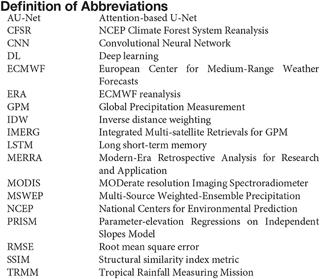
Appendix

Definition of Abbreviations