Spatially-Resolved Integrated Precipitation-Surface-Groundwater Water Isotope Mapping From Crowd Sourcing: Toward Understanding Water Cycling Across a Post-glacial Landscape

Isotopic analyses of δ¹⁸O and δ²H of water in the context of the hydrologic cycle have allowed hydrologists to better understand the portioning of water between the different water domains. Isoscapes on a large spatial scale have been created to show isotopic variation in waters as a function of elevation, temperature, distance to coast, and water vapor source. We present the spatial and temporal isotopic results of precipitation, surface water, and groundwater of an ongoing study across Massachusetts, USA in order to establish an isotopic baseline for the region. This represents one of the most comprehensive and detailed isotopic studies of water across a 10,000 sq mi area that has exhaustively sampled important components of the terrestrial hydrologic cycle (precipitation, groundwater, and surface waters). We leverage the support of volunteers and citizen scientists to crowd source samples for isotopic analysis. The database consists of water samples from 14 precipitation sites, 409 ground water sites and 516 surface water sites across the state of Massachusetts, USA. The results indicate that groundwater isotopic composition ranges from δ¹⁸O −11 to −4‰ surface water ranges from δ¹⁸O −13 to −3.84‰ and precipitation ranges from δ¹⁸O −17.88 to −2.89‰. On a first order, the small bias of mean groundwater (−8.7‰) and surface water (−8.0‰) isotopes compared to precipitation δ¹⁸O (−7.6‰) supports that groundwater recharge and surface water storage effects through the hydrologic year impact the isotopic composition of surface and groundwater. While differences are distinct, they are larger than previously reported values, but still suggest more importance of summer precipitation than previously acknowledged. On average seasonal amplitudes of precipitation (2.7‰), surface water (1.13‰), and groundwater (~0‰) of the region demonstrate young water fractions of surface water to be 40% with groundwater ~0%. Results demonstrate that mean δ¹⁸O in precipitation, surface water and groundwaters are more enriched in heavy isotopes in areas near the coast, than the interior and western portion of Massachusetts. The hope is for this dataset to become an important tool for water management and water resource assessment across the region.

Introduction

The exploration of the stable isotopes of water, oxygen, and hydrogen isotope measurements, have increasingly improved our understanding of the behavior of water isotopes on both a large and small scale. They have been widely used as tracers to better understand hydrological and meteorological processes. Numerous studies have used stable isotopes in hydrological (Kendall and Coplen, 2001; Jasechko et al., 2014, 2017; Landwehr et al., 2014; West et al., 2014; Yeh et al., 2014; Good et al., 2015; Birkel et al., 2018), meteorological (Gonfiantini et al., 2001; Celle-Jeanton et al., 2004; Dutton et al., 2005; Earman et al., 2006; Lachniet and Patterson, 2009; Puntsag et al., 2016; Ren et al., 2016), and paleoclimatology reconstruction studies (Dansgaard, 1964; Risi et al., 2010; Landais et al., 2017). Recently the stable isotopes of meteoric waters in continental environments have been used to make better interpretations related to climate and relationships between precipitation, surface water, and groundwater (Hervé-Fernández et al., 2016; Koeniger et al., 2016; Sprenger et al., 2016; Berry et al., 2017) both spatially and temporally.

Through the creation of isoscapes, defined here as a spatial and temporal distribution of water isotopes for a particular geographic region, local processes such as the interaction between surface and groundwater can provide spatial and temporal information that can be beneficial to water resources and management. Isoscapes are the end result of spatial and temporal distribution of isotopes, they are useful in describing environmental conditions across space and time (Bowen, 2010). They allow us to determine the interconnectivity in various systems, such ecological, hydrological, biogeochemical, or meteorological systems. Kendall and Coplen (2001) created an isoscape for δ¹⁸O and δ²H in river waters across the United States using precipitation isotope data collected from selected US Geological Survey water-quality monitoring sites. Through extensive analyses of δ¹⁸O and δ²H in both precipitation and surface waters this study revealed distinct spatial and temporal differences in δ¹⁸O and δ²H of both river and meteoric waters. State Meteoric Water Lines were created based on geographic regions across the US. A regional pattern within the State Meteoric Water Lines was noted suggesting the large geographic areas are controlled by the humidity of the local air mass which conveys an evaporative enrichment and thus in the stream samples within the area. Spatially the δ¹⁸O and δ²H in river waters fall along local water lines but also reveal a distinct correlation with topography and appear to be primarily reflecting the isotopic signal of precipitation. Jasechko et al. (2014) used 20 years of spatial and temporal data of the stable isotopes of water in groundwater, river water, and precipitation to determine seasonal bias in groundwater recharge and young streamflow in the Nelson River basin of west central Canada. Regionally in the northeastern US winter recharge ratios exceeds summer recharge ratios or the groundwater is biased by winter recharge (Jasechko et al., 2017). Cold-season recharge ratios were typically greater than warmer season recharge ratios and that precipitation which falls within the past 2 or 3 months make up about one-quarter of river discharge. Puntsag et al. (2016) examined a 43-year record of precipitation isotope values collected at the Hubbard Brook Experimental Forest in New Hampshire, US and noted a positive trend in the deuterium excess values and a negative trend in both the δ¹⁸O and δ²H. These trends were linked to increases in the interaction with air masses from the Atlantic Ocean and Arctic.

This study aims to examine the relationship between modern precipitation, surface water, and groundwater stable isotopes across Massachusetts (USA) via crowdsourcing to assess the isotopic variability of waters and relate variability to landscape and hydrological features. We also identify the spatial and temporal trends in seasonal surface and groundwater isotopes and 2-week weighted precipitation isotopes and distinguish hydrologic and hydrogeologic trends in surface and groundwater, respectively. Using these trends, we discuss and quantify the implications for either precipitation induced variability or variability due to open water systems, topographic differences, hydrogeologic and hydrologic processes in surface and groundwater stable isotopes. We envision that these datasets will allow us to address questions such as: (a) What is the nature of surface and groundwater interaction in the northeast US? (b) What are the potential impacts of climate change on stream flow generation, groundwater recharge, and groundwater storage? (c)How important are extreme precipitation events to groundwater storage? And (d) How does groundwater surface water interconnectivity change spatially across the landscape? Fundamentally, the use of stable water isotopes has become an inexpensive way to characterize the temporal and spatial variability of water bodies at a high resolution (Birkel et al., 2018) and can be used to inform management on both a local and regional scale.

Background

Stable Isotopes as Tracers

The interpretation and analysis of the composition of environmental water stable isotopes (precipitation, surface water, groundwater), δ¹⁸O and δ²H, are an important tool in examining the hydrologic processes on a global and regional scale (Dansgaard, 1964; Kendall and Coplen, 2001; Bowen, 2010; Puntsag et al., 2016). These analyses provide a better understanding for quantifying the spatially integrated effects of the water cycle and processes that occur in both the watershed and atmosphere (Bowen et al., 2011) as well as determining the relative amount of precipitation and groundwater in surface waters (Kendall and Coplen, 2001). Oxygen and hydrogen measurements of precipitation, surface water, and groundwater illustrate the effects of climate, topography, elevation, and various environmental parameters (Dansgaard, 1964; Lee et al., 2010; Welker, 2012; Evaristo et al., 2015; Akers et al., 2016).

Several studies have established that a variety of climatological, geological, biological, and hydrological effects on the stable isotopic composition of water (Gonfiantini et al., 2001; Reddy et al., 2006; McGuire and McDonnell, 2007; Botter et al., 2010; Bowen, 2010; Mueller Schmied et al., 2014; Akers et al., 2016; Puntsag et al., 2016; Ren et al., 2016; Sprenger et al., 2016). Such studies have determined a negative relationship between δ¹⁸O and elevation (Gonfiantini et al., 2001; Celle-Jeanton et al., 2004; Windhorst et al., 2013; Landwehr et al., 2014), a positive relationship between δ¹⁸O, temperature, distance inland, and latitude (Ingraham and Taylor, 1991; Welker, 2000; Dutton et al., 2005; Liu et al., 2010; Akers et al., 2016; Ren et al., 2016), and a correlation between water vapor source and δ¹⁸O (Timsic and Patterson, 2014; Puntsag et al., 2016).

Understanding the stable isotopes of water relies heavily on accurate and high precision measurements of δ¹⁸O and δ²H (Brand et al., 2009; Wassenaar et al., 2012). Isotope ratios are considered ideal tracers as they are part of the water molecule and can be easily sampled and preserved in groundwater, surface water, precipitation. Most importantly hydrogen and oxygen can preserve vital historical information (location, time, phase of precipitation) thus becoming a primary tool for hydrological, atmospheric, and meteorological studies (Reddy et al., 2006; Bowen et al., 2007; Timsic and Patterson, 2014). The stable isotopes of water are presented in the δ notation and represent the difference in heavy to light isotopes of water relative to the Vienna Standard Mean Ocean Water (VSMOW) (Craig, 1961; Sprenger et al., 2018). Although the delta notation is a dimensionless quantity the values are in per mil because of the low variation in the natural abundance of water stable isotopes (Kendall and Coplen, 2001; Sprenger et al., 2018). High d values indicate a higher ¹⁸O/¹⁶O and ²H/¹H ratio relative to the Vienna Standard Mean Ocean Water. Low d values indicate a lower ¹⁸O/¹⁶O and ²H/¹H ratio relative to the Vienna Standard Mean Ocean Water. For the purposes of this paper, the term “enriched” will be used to describe water samples that have a high amount of heavy isotopes and “depleted” will be used to describe water samples that have a low amount of heavy isotopes. To determine the δ¹⁸O and δ²H of a water sample Equation (1) is used:

$\begin{array}{ll}\delta =(\frac{{\text{R}}_{\text{Sample}}}{{\text{R}}_{\text{Standard}}}-1)\times 1000& (1)\end{array}$

where R is the abundance ratio of the heavy and light isotopes (e.g., ¹⁸O/¹⁶O and ²H/¹H) and Rstandard is the VSMOW.

In a dual isotope plot, δ¹⁸O –δ²H, the relationship between δ¹⁸O and δ²H is defined as the global meteoric water line (GMWL) (Craig, 1961) and is described by the following equation: isotopes. To determine the δ¹⁸O and δ²H of a water sample Equation (1) is used:

$\begin{array}{ll}{\delta }^2\text{H}=8{\delta }^{18}O+10& (2)\end{array}$

This equation represents the relationship of δ¹⁸O and δ²H of surface waters globally and is an approximation of the mean world annual amount-weighted precipitation (Timsic and Patterson, 2014). This relationship is a result from Rayleigh processes, which is directly affected by temperature and pressure conditions during phase changes between liquid water and water vapor (Dansgaard, 1964).

More recently, the stable isotopes of water are analyzed together with deuterium excess (d-excess), Equation (3), which was originally proposed by Dansgaard (1964).

$\begin{array}{ll}d-excess={\delta }^{2}H-8^{*}{\delta }^{18}O+10& (3)\end{array}$

d-excess is the y-intercept of the GMWL and is dependent on relative humidity, temperature, and kinetic isotope effects during evaporation (Kendall and Coplen, 2001).

Because of this, d-excess values are sensitive to evaporative processes and can be used to measure the contribution of evaporated moisture and allow for additional assessments of environmental conditions during the time of vapor formation or rainout. High d-excess values indicate more evaporated moisture has been added and low values indicate samples fractionated by evaporation (Kendall and Coplen, 2001; Timsic and Patterson, 2014).

The line condition excess (lc-excess) is the deviation from the local meteoric line rather than the GMWL and is a good indicator of evaporative fractionation (Birkel et al., 2018).

It is defined by: Lc-excess = δ²H – a δ¹⁸O – b where a and b are the slope and y-intercept, respectively, of the GMWL.

Study Site and Region

Massachusetts is located in the northeastern portion of the United States and borders the Atlantic Ocean. It occupies 27,340 square kilometers where most of the state lies north of 42° latitude In elevation, Massachusetts ranges from <152 to 1,063 m above sea level where the western portion is characterized as mountainous, the central portion as rolling hills and coast as flat land with marshes and small lakes and ponds (Boutt, 2017). Massachusetts lies in the prevailing westerlies, a region that is dominated by westerlies, generally eastward air movement and drier continental airflow (Weider and Boutt, 2010). Most of the precipitation events are sourced from colder regions: Arctic, Mid/North Atlantic and the Pacific. Massachusetts tends to see precipitation events that originate from the Arctic, Mid-Atlantic, North Atlantic, Pacific, Continental, and the Gulf of Mexico (Puntsag et al., 2016). Massachusetts receives ~1,000 mm of rain annually and on average temperatures range from as high as 26°C and low as −8°C. This temperature variability is due to variance in topography. Because of this snowfall amount varies across the state making it difficult to determine a snowfall average. The National Climatic Division Center divided the state into three climatological divisions: Climate Zone 1, Climate Zone 2, and Climate Zone 3 (NCDC). Throughout this paper these zones will be shortened to CZ1, CZ2, and CZ3. Though, according to the Koppen-Geiger Classification, Massachusetts has four climatological divisions with the fourth climate zone encompassing the coast and Cape Cod. For this study, we have grouped together Climate Zone 4 with Climate Zone 3, thus dividing Massachusetts into only three Climate Zones.

Methods

Most of the samples presented here were collected by volunteers representing different groups across the region. We provided and shipped volunteers with empty bottles, labels and standard sampling instructions. Samplers were instructed to fill bottles as full as possible and close the cap as tight as possible. Upon shipping back to us, we inspected all bottles and discard samples that were not more than 75% full (almost all bottles had no leaks). Repeat analyses monthly of stored samples show no evidence of evaporative enrichment. Inspection of isotopic results did not reveal any storage anomalies or sample irregularities. This was confirmed by replicate analysis and consistency of results from given locations or times of sampling. All isotope data presented here is reported in Supplementary Table 3.

Precipitation

Eleven sampling sites form the precipitation isoscape network presented here (Figure 1). Sampling for the precipitation network took place from March 2017 to March 2018 and is still ongoing. Each volunteer was supplied with thirty 30 mL high density polyethylene (HDPE) bottles, a small funnel, and a data collection sheet. Volunteers were asked to pour the contents of their rain gauge into a 1-L Nalgene bottle every day for a 2-week time increment. At the end of the 2 weeks, the contents of the 1-L Nalgene bottle were poured into one 30 mL bottle which would result in a 2-week composite sample. During the winter months, if there was snow, volunteers would place the snow into a saucepan and dip the bottom of the pan into hot tap water. The melted snow can then be measured by pouring it from the saucepan into the inner cylinder of the rain gauge. Every 6 months, volunteers would send their precipitation samples to the University of Massachusetts-Amherst. Sample bottles were stored in plastic bags between the time of receipt and analysis.

FIGURE 1

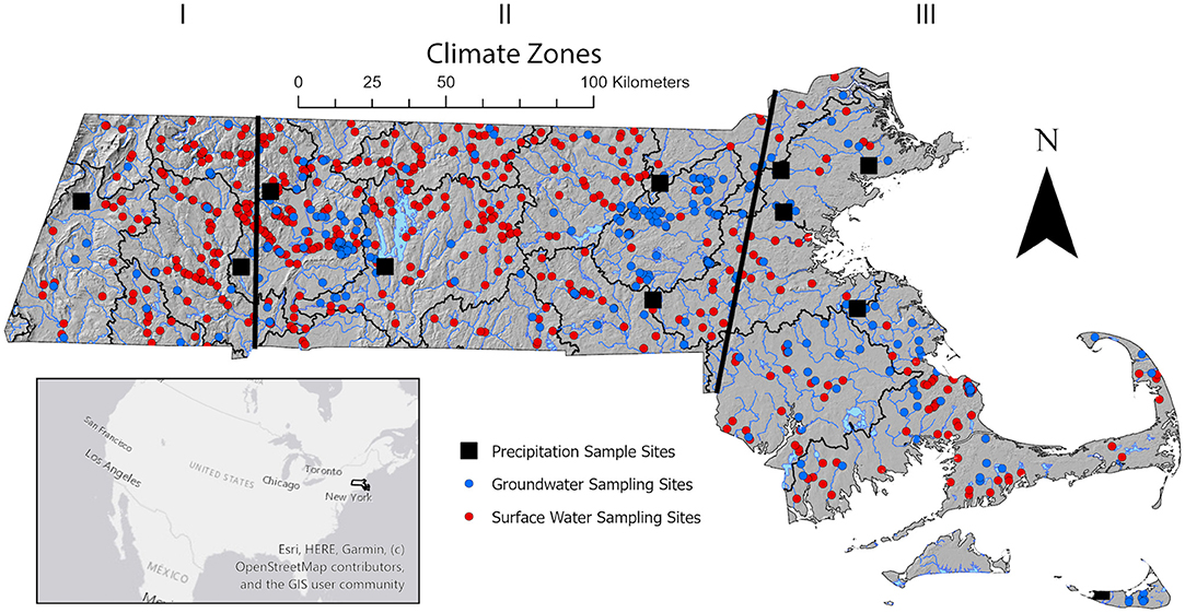
Figure 1. Site map showing geographic region of study including the location of precipitation sample collection sites (black squares), surface water sampling locations (red circles), and groundwater sample sites (blue circles). Climate zones are indicated as black lines delineating approximate boundaries.

Precipitation isotope analyses were screened and samples that had a deuterium excess <-10‰ were discarded as these may have been compromised by evaporation during storage/sampling. A total of 40 precipitation samples were removed from the analysis. After screening the precipitation isotope data we calculated a 2-week weighted averages following to remove any bias:

$\begin{array}{ll}Two-weekweighted\delta =P_{(2-\text{weeks})}x{\delta }^{2}Hor{\delta }^{18}O& (4)\end{array}$

Where P_(2−weeks) is the 2-week precipitation amount as provided by the volunteers. We then determined the average annual with a 2-week weighted average following

$\begin{array}{ll}{\delta }^{2}Hor{\delta }^{18}O={\displaystyle \sum }{P}_{\text{i}}/{\displaystyle \sum }{\delta }^{2}Hor{\delta }^{18}O& (5)\end{array}$

Where P_i is the sum of the precipitation amount of the sampling site.

Surface Water Sampling Network and Data Sources

One thousand nine hundred and seventeen surface water samples from 556 surface water sites (Figure 1) across Massachusetts were analyzed for δ¹⁸O and δ²H. Surface water sites were selected based on their spatial location in order to accurately represent a surface water isoscape for Massachusetts. Surface water samples were collected from 2011 to 2018. Samples were collected from faculty and students from the University of Massachusetts-Amherst, watershed associations (Nashua Watershed, Charles River Water, Blackstone, Quabbin, and Chicopee River Watershed), and the acid rain monitoring (ARM) project. Volunteers were supplied with 1 or more 15 mL high density polyethylene (HDPE) bottles and a data collection sheet. On the day of sampling, volunteers were asked to thoroughly clean out the HDPE bottle with the to be collected water and then refill the bottle to the top to limit the amount of headspace and securely fasten the cap. Samples were returned to the University of Massachusetts where they were prepared for analysis within a few weeks upon arrival. Sample bottles were stored in plastic bags between the time of receipt and analysis.

Groundwater Sampling Network and Data Sources

One thousand four hundred and six groundwater samples from 409 groundwater sites across Massachusetts were analyzed for δ¹⁸O and δ²H (Figure 1). Groundwater samples were collected from 2011 to 2018. Thirty-eight sites are from the US Geological Survey Eastern Massachusetts Water Monitoring (USGS-ESWM), six sites are from the US Geological Survey in Nantucket, 79 sites are from the US Geological Survey National Water Information System (USGS-NWIS), four are from the US Geological Survey Snow Pond, 95 sites are from the University of Massachusetts-Amherst database with sampling done by students and faculty, 71 sites are from Safewell (a well testing company for real estate transactions), and 126 sites are from volunteers across Massachusetts.

Each volunteer was supplied with 1 or more 15 mL high density polyethylene (HDPE) bottles and a data collection sheet. On the day of sampling, volunteers were asked to first run the tap water for a couple seconds, thoroughly clean out the bottle with the tap water and the fill the bottle to the top to limit the amount of headspace and securely fasten the cap. Samples were returned to the University of Massachusetts-Amherst where they were prepared for analysis within a few weeks upon arrival. Sample bottles were stored in plastic bags at room temperature between the time of receipt and analysis.

Analysis of Isotopic Composition of Water

Stable isotope compositions were measured by a wavelength scanned cavity ring-down spectrometry on un-acidified samples by a Picarro Cavity Ring Down Spectrometer (L2120-I) analyzer (Berden et al., 2000). Cavity ring-down spectroscopy is a direct absorbing technique which is conducted with eight pulse or continuous light sources which is significantly more sensitivity than the conventional absorption spectroscopy. The Picarro is equipped with a high precision vaporizer (A0211) and fitted with a CTC PAL auto-sampler. International reference standards (IAEA, 2000, Vienna, Austria) were used to calibrate the instrument to the VSMOW scale. To remove possible memory effect between samples, each sample was analyzed six times and the results of the first three injections were discarded. To further reduce memory effect, we adopted a modified version of a technique by Penna et al. (2012) where samples are grouped by water source and location. Three reference waters that isotopically bracket the sample values were run alternately with the water samples: Boulder, Colorado, Tallahassee, Florida and Amherst, Massachusetts, were used for a total of nine times each in every sample tray. The average values for these standards are −16.5, −2.6, and −7.5‰, respectively. These standards were calibrated with the Greenland Ice Sheet Precipitation (GISP), Standard Light Antarctic Precipitation (SLAP) and Vienna Standard Mean Ocean Water (VSMOW) from the IAEA (Kendall and Coplen, 2001). The results were calculated based on a rolling calibration so that each sample is determined by the three standards closest in time to that of the sample.

Results

Precipitation

Three-hundred and ninety four (394) precipitation analyses are presented in Figure 2 on a dual isotope plot. δ¹⁸O values range from −18 to −1.3‰, δ²H values range from −132 to −8.0‰ and d-excess values range from −7.3 to 44‰. Average δ¹⁸O, δ²H, and d-excess values are −7.6 (±3), −47 (±24), and 12 (±6)‰, respectively. The precipitation data points form a flattened ellipse on the GMWL. Most of the data points fall on the GMWL with a few plotting off onto the evaporative enrichment line (Figure 2).

FIGURE 2

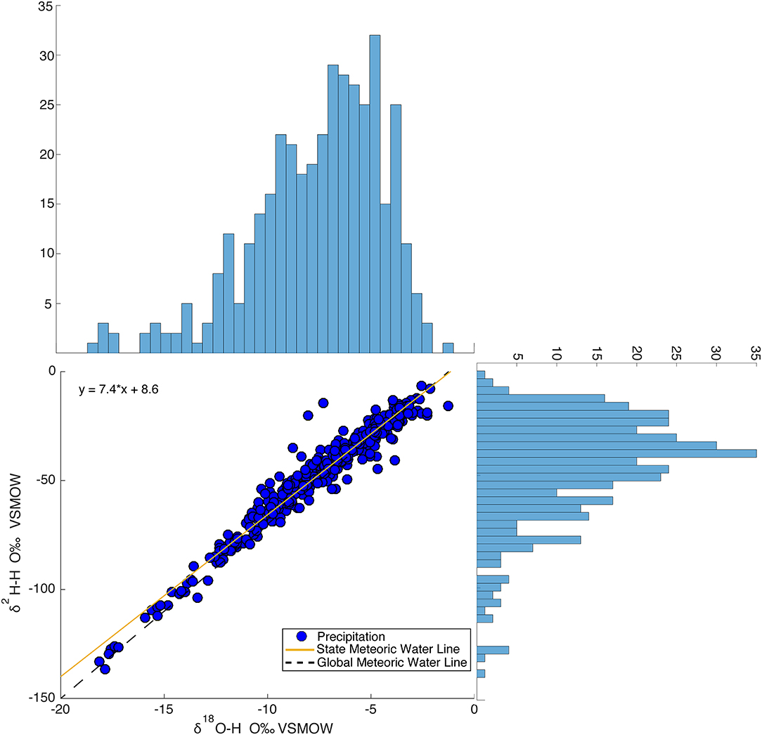
Figure 2. Dual isotope plot of samples in the isoscape precipitation network (394 precipitation samples, 11 sampling sites). The frequency of δ¹⁸O and δ²H are plotted on their respective axes.

The State Meteoric Water Line (SMWL) generated from the unweighted stable isotope values of the 394 precipitation samples is δ²H = 7.7^*δ¹⁸O + 9.8. This regression line is calculated based on binning the 394 precipitation samples 0.5‰ in δ¹⁸O and then averaging the values. This is performed because the density of enriched samples are biased in the dataset, and the resulting line better represents the SMWL across the full range of isotopic compositions observed.

We compare our precipitation isotope analyses with two precipitation sites from Massachusetts collected by Vachon (2007). Weighted monthly averages from our network were calculated and compared to the weighted monthly averages of MA13-Boston, MA01-Cape Cod. Standard deviations between our weighted monthly averages and the weighted monthly averages of MA13 and MA01 ranged from 1.9 to 0.2‰.

Following the methods of von Freyberg et al. (2018), using the equation below, a sine-wave was fitted through the reported precipitation isotope values to better quantify the seasonal isotope cycles.

$\begin{array}{ll}C\text{p(t)}=A_{\text{p}}sin(2\pi f\text{t}--\phi \text{P})+k\text{P}& (6)\end{array}$

In Equations (6) and (7), A_p is the amplitude for precipitation (‰), φ is the phase of the seasonal cycle, t is the time in years, is the frequency (yr⁻¹), and k (‰) is a constant which describes the vertical offset of the isotope signal (von Freyberg et al., 2018). These equations allow us to quantify the amplitude of the seasonal isotope cycles and the coefficients, a, b, and c by using multiple linear regressions where a, b, and c are the amplitude, phase, and offset, respectively.

$\begin{array}{ll}C\text{p(t)}=a_{\text{p}}cos(2\pi f\text{t})+b_{p}sin(2\pi f\text{t})+c\text{P}& (7)\end{array}$

The amplitude A_p is then determine by:

$\begin{array}{ll}Ap=\sqrt{a_p^2+b_p^2}& (8)\end{array}$

Using these equations, we fit sine curves to the isotope data for all the precipitation isoscape samples, as well as each individual station (Figure 3). We found the equation of the sine fitted line to be:

FIGURE 3

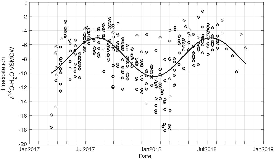
Figure 3. Time series of precipitation δ¹⁸O isotopic analyses with a seasonal fitted black line (equation in text) using non-linear least squares method. Amplitude of the seasonal fluctuation is 2.7‰ for δ¹⁸O.

$Cp(t)=-2.07cos2\pi \times \frac{1}{365}x\times -1.88sin2\pi \times \frac{1}{365}x+-7.82.$ Precipitation varies approximately −5.4‰ seasonally.

Amplitudes and offsets for each of the 11 precipitation sites were determined and compared with the calculated amplitudes and offsets of MA01 and MA13 (Vachon, 2007) to compare to our calculated values. The amplitude for each of our precipitation site ranges from 2.14 to 4.00 (±0.66) and the offset ranges from −6.12 to −9.39‰ (±0.99).

Additionally, seasonal local meteoric water lines were determined for winter and summer. Winter months includes October to March and summer months includes April to September. The LMWL for summer generated from the unweighted stable isotope values sampled during the summer months is δ²H = 6.6^*δ¹⁸O + 2.6. The LMWL for winter is δ²H = 7.4^*δ¹⁸O + 11. The slope, y-intercept, and d-excess of the winter LMWL is larger than the slope and y-intercept of the summer LMWL.

Median, minimum and maximum δ¹⁸O values were determined over a 12-month period and correlated to determine any statistical significance associated over this period, Figure 4. Over this 12-month interval, the δ¹⁸O values are variable where on average there is a −5.4‰ range. This same method was performed on the δ²H values, though it was determined that this plot illustrated similar patterns to that of the box plot of δ¹⁸O values and did not illustrate any new information. Over a 12-month period δ¹⁸O values steadily decreased from September to March and then drastically increased from March to April where values continued to increase from April to May. Between May and June δ¹⁸O values decreased and then increased from June to August. Maximum δ¹⁸O values occur during the late summer and early fall months and minimum δ¹⁸O values occur during the late winter and early spring months, specifically March. These trends are relatively correlated with temperature (Cole, 2019).

FIGURE 4

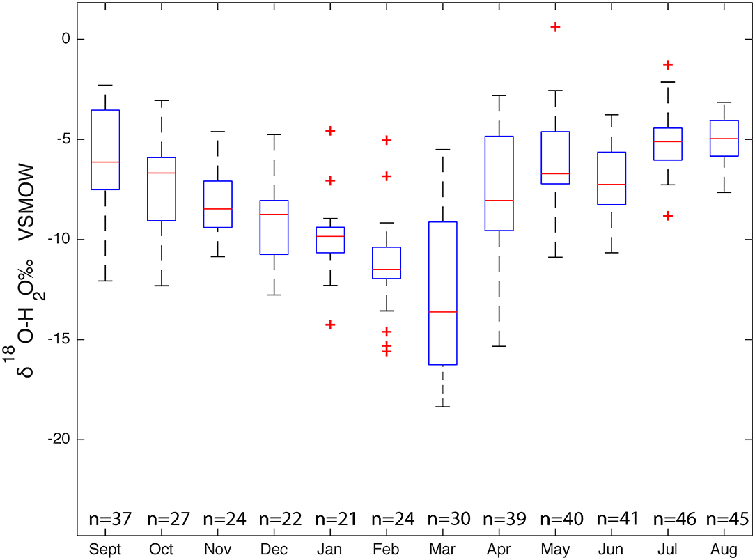
Figure 4. Box plot of δ¹⁸O precipitation values across the hydrologic year.

To assess the role of climatic variability on isotopic compositions, all precipitation samples were categorized into climate zones (Table 1). A trend toward more enriched precipitation values is observed moving from west to east across the study site (climate zones 1–3). Two-week weighted averages were determined for each of the 11 precipitation sampling sites, grouped into their respective climate zones and then related to their respective elevation (Figure 5). Elevations within the sampling sites range from 4 to 331 m. MA01 (Cape Cod) and MA13 (Boston) from Vachon (2007) were plotted alongside our sampling sites and categorized into CZ3. Sampling sites located at a higher elevations and in CZ1 and are more depleted than samples located at a lower elevation CZ3 which are more enriched.

TABLE 1

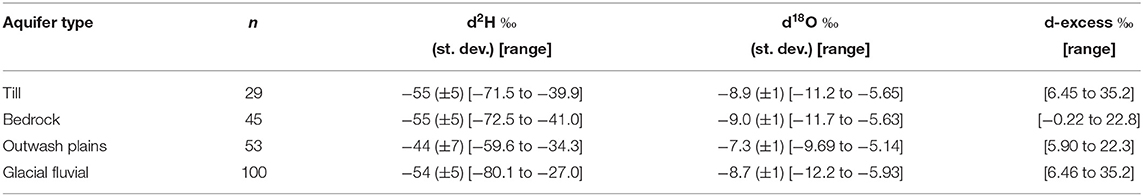
Table 1. Summary statistics of isotopic values of aquifer materials.

FIGURE 5

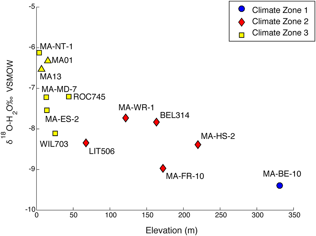
Figure 5. Relation of 2-week weighted total averages of the 11 precipitation sites with elevation. Precipitation sites are categorized based on climate zone location. Sample sites from Vachon (2007), are illustrated by triangles.

Local meteoric water lines (LMWLs) were calculated for each of the climate zones. The climate zone 1 LMWL generated from the 31 samples located in that region is δ²H = 7.8^*δ¹⁸O + 13, climate zone 2 LMWL generated from the 186 samples located in that region is δ²H = 7.5^*δ¹⁸O + 9.3 and the climate zone 2 LMWL generated from the 178 samples located in that region is δ²H = 7.4^*δ¹⁸O + 8.1.

These maximum and minimum δ¹⁸O values are primarily driven by temperature and moisture source differences. National Oceanographic and Atmospheric Administration Air Resources Laboratory Hybrid Single-Particle Lagrangian Integrated Trajectory (HYSPLIT; Draxler and Rolph, 2003) models were run for one station in each of the climate zones for the month of March and June in 2018. These months were chosen as they exhibited the largest difference in δ¹⁸O values. A total of six trajectory analyses were performed. Stations MA-BE-10 (CZ1), BEL314 (CZ2), and MA-NT-1(CZ3) were used for the HYSPLIT models. Model results indicate that in March all three stations saw air masses sourced from the continent and in June all stations saw air masses sourced from the Mid-Atlantic. Average monthly air temperature data was collected from the NOAA National Centers for environmental information, Climate at a Glance: Statewide Mapping from 2017 to 2018 as that time period encompasses the sampling period for the precipitation samples. Two-week weighted monthly δ¹⁸O averages were correlated with temperature and time of year. A positive correlation with δ¹⁸O values and temperature demonstrates an enrichment as temperature increases. The isotopic values are more variable at cooler temperatures and less variable at warmer temperatures. A good agreement between isotopic composition and temperature where temperature follows the same δ¹⁸O temporal pattern but with some offset.

Surface Water

The δ¹⁸O values of the 1,707 surface samples across Massachusetts range from −13.0 to −3.48‰, δ²H values range from −84.3 to −16.3‰, d-excess values range from −9.72 to 24.9‰, and lc-excess values range from −20.8 to 12.2‰. The dataset forms a flattened ellipse that lies slightly above and angled to the SMWL, Figure 6 illustrates the isotopic variability. The data points that fall above the SMWL indicate high deuterium excess values and sample points that fall off the SWML, indicate open system enrichment. A histogram for both δ¹⁸O and δ²H were plotted and juxtaposed with the dual isotope plot of surface water analyses to illustrate the distribution and frequency of the δ¹⁸O and δ²H values. At approximately δ¹⁸O −6‰ and δ²H −45‰ there is an increase in the number of surface water samples, indicating where surface water samples start to plot off the SMWL. Average δ¹⁸O, δ²H, and d-excess values for surface water are 8.0 (±1), 50.0 (±8), and 14.1 (±4)‰, respectively. The Surface Water Line (SWL), which is the unweighted linear regression generated from the 1,707 surface water samples is δ²H = 5.7^*δ¹⁸O - 4.2. To determine seasonal variability and its effect on surface water, samples were grouped by sampling month. Medians, minimum, maximum, 25th and 75th percentile, and 1% interquartile ranges were determined for each of the 12 months. Figure 7 illustrates that the δ¹⁸O values of surface water experiences seasonal variability where samples experience a depletion and enrichment throughout a hydrologic year. A similar plot for δ²H shows similar patterns as the δ¹⁸O plot.

FIGURE 6

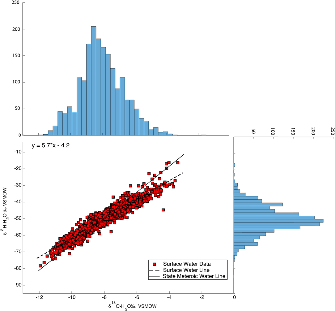
Figure 6. Relation between δ¹⁸O and δ²H surface water values for the entire dataset (1,917 surface water samples 556 surface water sites) with histograms of δ¹⁸O and δ²H on their respective axes.

FIGURE 7

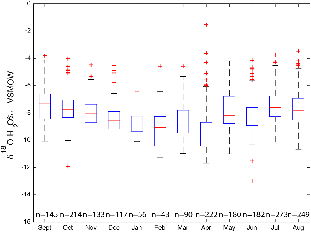
Figure 7. Comparison of δ¹⁸O values in surface water samples (1,917 samples) across the hydrologic year.

From September to February the δ¹⁸O median values decrease and then slightly increase in March and decreases again in April. From April to August δ¹⁸O values slowly increase. Because each sampling did not have a consistent number of samples, there will be is an inherent bias between months with a larger number of samples and those with a smaller number of samples. A Sine function was fit through the reported surface water isotope values sampled from 2016 to 2018 as most of the surface water sampling took place during this time. A sine wave fit was used to describe the seasonal isotope cycles:

$\begin{array}{r}Cp(t)=-0.45\cos 2\pi \times \frac{1}{365}x\\ \times -1.03\sin 2\pi \times \frac{1}{365}x+-8.48\text{.}& (9)\end{array}$

Using Equation (8), we found the amplitude of the sine curve to be 1.13‰, illustrated in Figure 8. Surface water experiences a seasonal range of 2.26‰ in δ¹⁸O.

FIGURE 8

Figure 8. Time series of surface water isotopic analyses with a seasonal fitted red line using non-linear least squares method where the amplitude is 1.13‰ for δ¹⁸O. Precipitation seasonal fit to data shown (from Figure 3) in black solid line, with dashed line extrapolated.

Groundwater

The δ¹⁸O values of the 1,405 groundwater samples across Massachusetts range from −12.2 to −5.07‰, δ²H values range from −80.1 to −35.5‰, and d-excess values range from −0.2 to 35.2‰. The dataset forms a flattened ellipse that lies slightly angled to the SMWL (Figure 9) with a higher percentage of points plotting off the SMWL and a few plotting off onto the evaporative enrichment line.

FIGURE 9

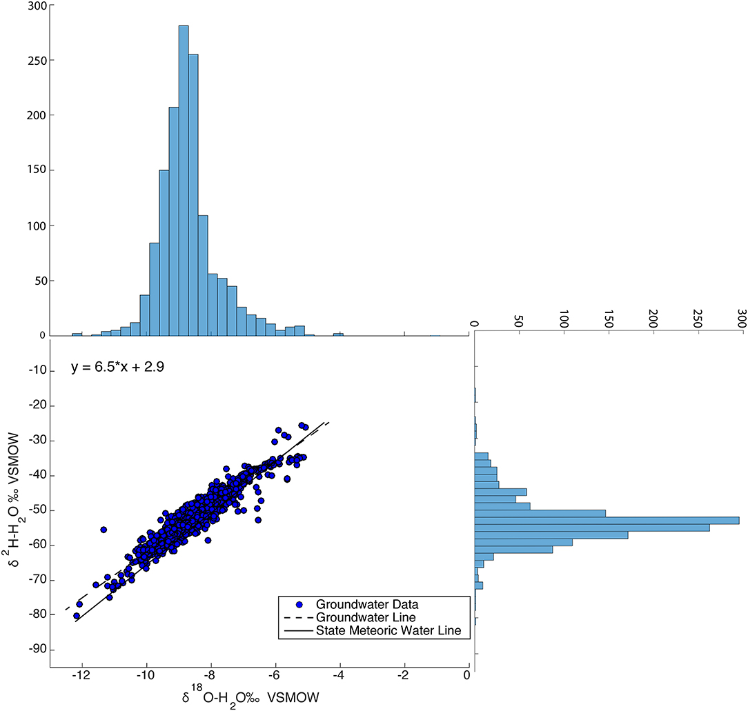
Figure 9. Relation between δ¹⁸O and δ²H groundwater values for the entire dataset (1,405 groundwater samples and 409 groundwater sites) with histograms of δ¹⁸O and δ²H on their respective axes.

Average δ¹⁸O, δ²H, and d-excess values for groundwater are 8.7 (±1), 53.3 (±6), and 16.3 (±4)‰, respectively. In order to better show the isotopic variability in groundwater, a histogram, which shows the frequency and distribution for both δ¹⁸O and δ²H were plotted and placed on appropriate axes with the dual isotope plot of groundwater analyses. At approximately δ²H −45‰ there is slight increase in the number of groundwater samples, this indicates where on the dual isotope plot groundwater samples start to fall off the SMWL and onto the evaporative enrichment line. The Groundwater Water Line (GWL), which is the unweighted linear regression generated from the 1,405 groundwater analyses is δ²H = 6.5^*δ¹⁸O + 2.9. The slope of the GWL equation is 6.5 and the y-intercept of intercept is 2.9.

To visually represent seasonal variability of groundwater, the unweighted δ¹⁸O and δ²H values of the groundwater samples were compared with the time of sampling. Medians, minimum, maximum, 25th and 75th percentile, and 1% interquartile ranges were determined for each of the 12 months. Figure 10 illustrates little isotopic variability between the medians of each month and indicates relatively homogenous seasonal variations in the unweighted δ¹⁸O values. A sine-wave was fit through the reported groundwater isotope values to better describe the seasonal isotope cycles: $Cp(t)=0.05cos2\pi \times \frac{1}{365}x$ × −0.04 $sin2\pi \times \frac{1}{365}x+-8.79$. Using Equation (8), we found the amplitude of the sine curve to be 0.07‰. Regionally groundwater experiences very little variability, with a seasonal range of 0.14‰.

FIGURE 10

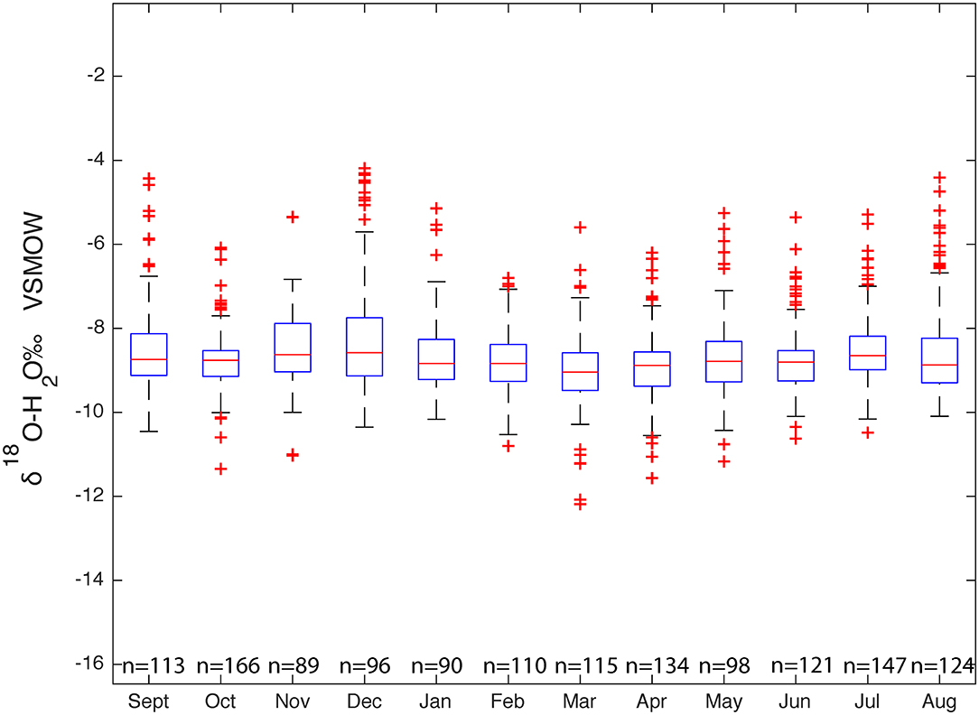
Figure 10. Comparison of groundwater δ¹⁸O values (1,405 samples) across the hydrologic year.

Groundwater samples were grouped based on the aquifer they were sampled in: glacial till, outwash plain, bedrock, and glacial fluvial deposits. Out of the 1,405 groundwater samples the aquifer for 44 of the samples were unknown. Statistics of groundwater isotopic compositions are summarized in Table 1 and all data is plotted as a function of aquifer geologic type are shown in the dual isotope plot Figure 11. Samples located in outwash plains with a few samples from glacial fluvial aquifers plot off the SMWL. Outwash fluvial, and bedrock aquifers are isotopically very similar, while outwash plains are the most enriched.

FIGURE 11

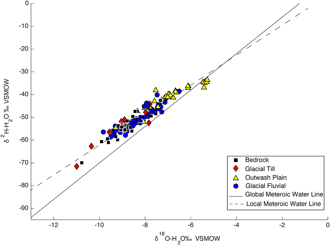
Figure 11. Isotopic composition of groundwater plotted as function of geologic deposit of sample.

Groundwater average δ¹⁸O values for each site were analyzed as a function of elevation to determine elevation effects. The elevation of groundwater samples ranges from 22 to 677 meters. Groundwater samples located at a lower elevation are more enriched than samples located at a higher elevation which are depleted. From 22 to 100 meters, δ¹⁸O values decrease from −3 to approximately −8‰. From 100 meters to 700 meters, δ¹⁸O values show some variability but are relatively similar at around −9‰.

Discussion

Comparison of SMWL, SWL, and GWL and Isotopic Variability

Important differences in the composition of isotopes were observed between precipitation, surface water, and groundwater. The SMWL is δ²H = 7.7^*δ¹⁸O + 9.8, the SWL is δ²H = 5.7^*δ¹⁸O - 4.2, and the GWL is δ²H = 6.5^*δ¹⁸O + 2.9, each line having its own unique slope and y-intercept (Table 1). Figure 12 illustrates the comparison between the SMWL, SWL and GWL and includes the 95th percent confidence interval for all three which was calculated using the curve fitting tool in MATLAB. The 95th percent confidence interval illustrates the minimum, maximum values and the range of variability for precipitation, surface water, and groundwater. These values and ranges allow us to compare and determine how variable the isotopic composition of δ¹⁸O and δ²H for precipitation, surface water and groundwater samples. The isotopic composition of precipitation across Massachusetts is more variable than groundwater and surface water. Both groundwater and surface water across Massachusetts experience some but smaller isotopic variability. Both the SWL and the GWL have shallower slopes than the SMWL and have an imbricate nature relative to the SMWL, Figure 12.

FIGURE 12

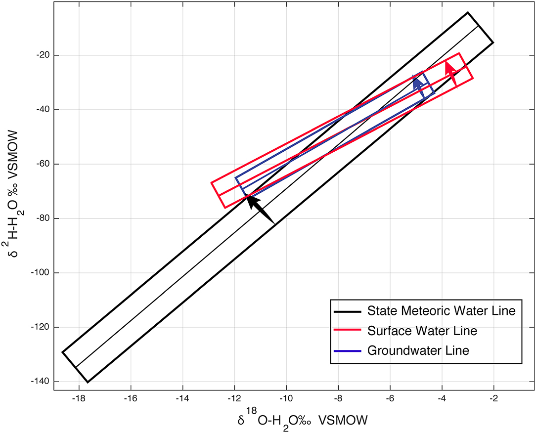
Figure 12. 95% confidence interval comparison between the SMWL, SWL and GWL. The arrows indicate low to highest values within the 95% confidence interval polygon.

These differences reflect local precipitation processes but also reveal the correlation between precipitation, surface water and groundwater. Because the slope of the SWL and the GWL are both pulled toward the line of evaporative enrichment, it can be determined that the slope of both these lines are biased by evaporation in an open water system. The slope of the GWL is larger than the SWL but smaller than the SMWL. This is telling that groundwater is composed of some fraction of precipitation and surface. Although surface water is more variable than groundwater, the isotopic composition of groundwater have similar ranges, meteoric water line slope, and averages compared to surface water. Though in order to determine the fraction of surface water to precipitation in groundwater, a data comparison between modeled and observed analyses would have to be performed. As noted, the slope of the SWL is shallower than both the SMWL and the GWL. The isotopic composition of surface water is affected by both the isotopic composition of precipitation, the isotopic composition of groundwater, and open vs. closed water systems. As a result of this, the isotopic composition of surface water will be inherently weighted by precipitation and groundwater (Dutton et al., 2005) and it might be expected for the SWL to be more similar to the SMWL. From Kendall and Coplen (2001) low slopes of the LMWLs may be suggestive of post-rain evaporative enrichment which can be reflected in the surface water. The slope of the SWL is drawn downward and biased possibly by open water enrichment. In a study performed by Kendall and Coplen in 2001, LMWLs are likely to have slopes as low as 5 to 6 in arid regions where summer rains are primarily derived from the Gulf of Mexico and are the main source of recharge to surface water. Kendall and Coplen (2001) stated that many of the surface water samples, especially in arid zones, show LMWL slopes <6 are indicative of evaporation. Interestingly they found that most of the eastern sites in their study had slopes that range between 7 and 8 and have intercepts that ranged from 5 to 12‰. The slope of the SWL in Massachusetts is 5.7, which, as suggested by Kendall and Coplen (2001) indicates significant evaporation. As evidenced by the trend in isotope values in Figure 6, some surface water samples fall off and to the right of the meteoric water line (d-excess <10). Samples with these values are primarily from waters in the southeast part of the state with a preponderance of open surface water bodies.

Alternatively, one consideration that hasn't been discussed are anthropogenic affects such as the presence of dams or impoundments, which are present in some of the rivers and reservoirs included in this study. Dams naturally increase evaporation, thus rivers or reservoirs associated with these dams will produce an evaporative signal and cause the δ¹⁸O values of surface waters associated with these dams to be high. This in effect will cause the recycling of surface water that already have high δ¹⁸O values to move through the hydrologic cycle where further enrichment of δ¹⁸O values may take place. Another consideration is the order of the rivers and/or streams and the size of the catchment of the rivers. When we compare the slope of the GWL to the SMWL and the SWL, we find that it lies between both the SMWL and the SWL. With the exception of <5% of the groundwater samples, most of the samples lie above the SMWL indicating high d-excess values. Those samples that have δ²H and δ¹⁸O values that lie below the SMWL and onto the evaporative enrichment line are indicative of samples that have gone through isotopic fractionation. Most of the groundwater samples that have an evaporative signal are located in CZ 3 where outwash plain aquifers are located and are only found in the southeast portion of Massachusetts. Outwash plains in the southeast portion of Massachusetts have a high amount of surface water features such as kettles lakes and ponds where ponds are essentially the water table. This could cause a high amount of groundwater surface water variability. As demonstrated in Figure 11, outwash plains are the most enriched and also the most variable. This portion of Massachusetts was located near the terminus of an ice sheet and consists of sandy terminal moraines. Because of the permeable nature of the aquifer, an estimated 45% of the average annual precipitation percolates into the soil and becomes groundwater recharge and an estimated 55% of the precipitation is evaporated (Olcott, 1995).

Figure 13A illustrates the distribution and variability of δ¹⁸O values for weighted precipitation, surface water, and groundwater. The median for groundwater, surface water, and precipitation are −8.78, −8.16, and −6.88‰, respectively. The positive ends of the surface water and groundwater plot are influenced by more enriched precipitation. This offset reveals that the isotopic signal of precipitation becomes filtered due to recharge infiltration, evaporation, and evapotranspiration and is reflected in the surface and groundwater. The depleted values in both the surface water and the groundwater are suggested to be primarily due to snowmelt and winter precipitation events.

FIGURE 13

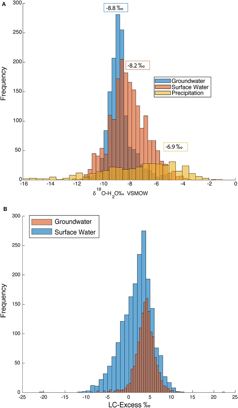
Figure 13. (A) Histogram of δ¹⁸O for groundwater (1,403 samples), surface water (1,917 samples), and precipitation (394 samples). Median values are indicated above data in color coded boxes. (B) Histogram of LC-excess values for both groundwater and surface water.

Lc-excess was calculated for both groundwater and surface water to define the number of groundwater and surface water samples that have gone through evaporative enrichment. Negative lc-excess values indicate evaporative enrichment and positive lc-excess values indicate differences in moisture source (Birkel et al., 2018). From Figure 13B it can be shown that approximately one quarter and one eighth of surface water and groundwater samples, respectively, have lc-excess values less than zero. Though it is no surprise that there are more surface water samples with higher lc-excess values than groundwater samples because surface water samples experience more isotopic fractionation than groundwater. We found that the SMWL for precipitation to be almost identical to the global meteoric water line. The global meteoric water line (GMWL) is defined as δ²H = 8^*δ¹⁸O + 10 and the SMWL is δ²H = 7.7^*δ¹⁸O + 9.8. When compared to the GMWL, the slope and y-intercept is less than the GMWL. Differences in slopes could be to in-cloud processes such as sub-cloud evaporation, evaporation during rainfall, or intensity of rainfall (Ren et al., 2016).

Seasonal and Hydrologic and Hydrogeologic Effects

Precipitation

Precipitation experiences a seasonal isotopic enrichment and depletion in the heavy isotopes. During the summer and spring months storms are primarily sourced from areas where temperatures are high and the isotopic composition of water vapor are more enriched. The moisture that becomes precipitation is usually sourced from surface water at mid to low latitude oceans where elevation is low and temperatures are high and evaporation occurs from the continents (Welker, 2012). During the winter months snow is the primary mode of precipitation. Massachusetts sees Nor'easters, which are storms that are sourced from the Mid-Atlantic and are formed due to the sharp contrast in temperature between the Gulf stream current and the cold air masses from Canada. Due to the formation of these storms, the storms will produce isotopically depleted precipitation. Typically, precipitation events during winter months are sourced from surface water at high latitudes and high elevations where temperatures are cold. For the most part precipitation in the Northeast is advected from the Gulf of Mexico, Mid-Atlantic, Pacific, Arctic, North Atlantic, and Continental (Welker, 2000).

Many researchers have determined and documented significant differences between the isotopic compositions of winter vs. summer precipitation (Birkel et al., 2018, von Freyberg et al., 2018). Birkel et al. (2018) determined the LMWLs for fall, winter, spring, and summer for 22 catchments in Scotland and found that between all the seasons winter had a larger slope than summer. Winter and summer meteoric water line were determined for the 394 precipitation samples in our precipitation isoscape network. Similar to the findings of Birkel et al. (2018), the slope of the winter meteoric water line is larger than the slope of the summer meteoric water line.

These differences are primarily due to seasonal differences in stormtracks, but can also be due to seasonal changes at the precipitation site (Kendall and Coplen, 2001) and reflect changes in source and temperature during a hydrologic year. In Massachusetts, there is a seasonal temperature discrepancy between summer and winter months. Average monthly temperatures were collected from the NOAA National Centers for Environmental information, Climate at a Glance: Global Time Series. The average temperature for summer, which is defined as April to September (Jasechko et al., 2014) is 16°C and average winter, which is defined as October to March (Jasechko et al., 2014) temperature is 3°C (NCDC). It is documented that air temperature and average 2-week weighted monthly δ¹⁸O values have a positive correlation. As temperature increases precipitation becomes isotopically enriched and vice versa. At higher temperatures, the variability is less compared to lower temperatures where there is a larger amount of variability. This is primarily due to seasonal moisture source differences. HYSPLIT models shows that in the first week of March 2018, all sampling sites experienced precipitation events that originated from a continental source, had a more northerly route and experienced cooler temperatures and more moisture recycling due to the fact that the air mass had a continental pathway.

Surface Water

A seasonal trend was documented for our entire surface water dataset. During the summer months (April to September) surface waters experienced isotopic enrichment and during the winter months (October to March) surface waters experienced an isotopic depletion, Figure 7. April experienced the lowest δ¹⁸O values while September experienced the highest δ¹⁸O values. Interestingly, as mentioned above summer is defined by the months of April to September and winter is defined by the months of October to March; though it is the month of April that experiences the most isotopic depletion. One possible explanation for this difference is differential recharge or delayed snowmelt (von Freyberg et al., 2018). The average temperature of March in Massachusetts is ~0°C while the average temperature of April is ~10 °C. This temperature difference could cause snow to melt much later in the winter season and into early spring. Because of the late snowmelt, surface water would experience recharge that has lower δ¹⁸O values. Dettinger and Diaz (2000) found that in the eastern United States the amount of precipitation entering streams is higher during the winter months than the summer months.

Modifications in isotope composition is impacted by evaporative enrichment during summer months, the amount of enrichment due to surface water type (stream vs. pond/lake), and the source of precipitation all affect the slope the SWL. δ¹⁸O comparisons for each sampling month show a large number of surface water samples experience enrichment in the heavy isotopes and plot above the 1% interquartile range. One possible explanation for these outliers are that these samples experienced open water enrichment isotopic fractionation causing sample to become isotopically enriched. Alternatively, these samples could be the result of additions of isotopically enriched precipitation. Samples categorized based on the type of surface water show that the δ¹⁸O values of each type lakes, reservoirs, and ponds were more variable (and show more d-excess and enrichment off of the SMWL) than rivers, streams, and springs.

In order to investigate whether precipitation or open water enrichment are the primary effects that cause surface water isotopic variability we used the amplitudes calculated from the sine-wave fit lines in both precipitation and surface water to determine the fraction of young water to precipitation. As defined by von Freyberg et al. (2018) the young water fraction is the proportion of catchment discharge that is younger than 2–3 months and can be approximated from the amplitudes of seasonal cycles of stable water isotopes in precipitation and surface water. Young water fractions have been inversely correlated with water table depth and topographic gradients (Jasechko et al., 2014) and have become a useful value for catchment inter-comparison as well as catchment characteristics as it can be calculated from limited data (von Freyberg et al., 2018). By looking at the seasonal isotopic composition of precipitation one can determine the damping and phase shift of the seasonal cycle as it gets propagated through the catchment which can be used to determine the timing of catchments (von Freyberg et al., 2018). Higher stream flows will have larger young water fractions as an increase in stream discharge due to rain events will contain more recent precipitation than base flow. Lower stream flows will have smaller young water fractions and will contain more base flow.

From our data we find the amplitude of the mean δ¹⁸O of precipitation is 2.7‰ and the mean amplitude of δ¹⁸O of surface water to be 1.13‰. To calculate the fraction of young water to precipitation we used the following equation (von Freyberg et al., 2018) below where Ap and As are the amplitude of precipitation and surface water respectively: Fraction of young water = As/Ap. From our date we calculate the average fraction of young stream water to be 0.4. This value indicates that ~40% of total discharge is composed of “young waters” or water that is <2–3 months in age.

Surface water follows the same seasonal enrichment and depletion as precipitation but dampened, with a smaller amplitude (Figure 8). The phase shift between precipitation and surface water is very small, almost non-existent. This is likely due to a delayed release of depleted winter precipitation from snowpack (von Freyberg et al., 2018). A smaller damping also implies a smaller fraction of young water in the stream flow, a smaller proportion of modern water to base flow (von Freyberg et al., 2018). The lack of phase shift between the seasonal cycles of surface water and precipitation along with the calculations to determine the young water fraction, implies that surface water has a higher proportion of modern water to base flow.

Residual corrected model values compiled from Bowen et al. (2011) were compared with surface water data presented here in order to evaluate how variable observed values are with modeled isotopic values. Based on results reported here, surface water δ¹⁸O and δ²H values do not agree with the Bowen et al. (2011) simulated δ¹⁸O and δ²H values and that samples are biased by higher δ¹⁸O or δ²H values. Surface water δ¹⁸O and δ²H values are more enriched, than the residually corrected δ¹⁸O and δ²H values. Many of the data points lie within the seasonal variability range, suggesting a strong role of evaporation enrichment. P:PET induced seasonal variability is a primary control on surface water variability. Data points that plot outside of the seasonal range is indicative of open system enrichment (i.e., evaporative enrichment). These results suggests that 90% of surface water variability is due to P:PET induced seasonality and 10% is due to open system induced variability.

Groundwater

Global seasonal groundwater recharge (Jasechko et al., 2014) calculated by using the seasonal differences in groundwater recharge ratios between the summer and winter seasons are helpful for assessing water resource dynamics. Based on the calculated groundwater recharge ratio (Jasechko et al., 2014), recharge in eastern Massachusetts have winter time groundwater recharge ratios that are consistently higher than summertime recharge ratios. Temperate regions, which includes eastern Massachusetts, that a large percent of winter precipitation infiltrates and recharges aquifers relative to summer precipitation. Our data presented here (based on many samples) suggests larger magnitude of bias toward winter time recharge. For example the mean δ¹⁸O of precipitation we report here is −7.6‰ compared to groundwater mean δ¹⁸O of −8.7‰ (Table 1). Jasechko et al. (2014) reports similar mean isotopic composition of precipitation of −7.5‰ with a groundwater composition of −7.9‰. This bias is not necessarily even across the 3 climate zones. Strong variations in the isotopic composition of the more topographically varied climate zone 1 may explain the fact that the mean δ¹⁸O of precipitation in climate zone 1 being −9.3‰ compared to −9.1‰ for groundwater may suggest some landscape control on compositions and inferred differences. Additionally, the dataset does suggest that late-summer growing season high intensity precipitation events may be an important contributor to groundwater recharge (e.g., Boutt et al., 2019).

The four types of geologic deposits in the region (glacial till, glacial fluvial, bedrock, and outwash plains) have unique characteristics, properties and isotopic compositions. Outwash plains have the highest average δ¹⁸O value, glacial till, glacial fluvial, and bedrock have similar average δ¹⁸O values and are the most depleted. Most of the enriched samples plot higher than the 1% interquartile range, suggesting these samples are most likely groundwater that have experienced some sort of fractionation. Outliers that plot below the 1% interquartile range δ¹⁸O value could be representative of the isotopic composition of direct recharge via snow melt. Groundwater located in outwash plains are more variable than bedrock, glacial fluvial, and glacial tills. In the regions bedrock aquifers, which are dominated by fractured crystalline rock, they do not recharge quickly as the movement of water is controlled by the existence of secondary openings in the aquifer, which can create long residences time flow paths (Weider and Boutt, 2010). Groundwater in bedrock aquifers have a long residence time because of its low permeability. Till aquifers are located at higher elevations and primarily in recharge areas (Weider and Boutt, 2010). They tend to be thin and consist of unconsolidated material and drain and fill seasonally due to the permeability and porosity of the aquifer material. Stratified glacial fluvial aquifers are found in valleys and areas near streams. They tend to have a larger storage capacity than till aquifers (Weider and Boutt, 2010). These hydrogeologic properties as well as their water storage capacity are the determinant factors of groundwater and surface water interaction and may be an implication as to the lack of seasonal variability seen in the groundwater δ¹⁸O values.

Unlike precipitation and surface water, groundwater does not experience a statistically-observable seasonal isotopic enrichment and depletion due to what is known as a reservoir effect which indicates a well-mixed reservoir of groundwater. The young water fraction for groundwater was also determined and calculated to be ~0.02‰ which indicates that 2.60% of groundwater is <2–3 months in age. This lack of seasonal variability can also be due to a small seasonal input which can be further dampened by groundwater residence time being higher than the volume of the groundwater storage. δ¹⁸O values for each sampling month were compared to one another. In general, the groundwater δ¹⁸O values for each sampling month does not show any significant enrichment or depletion during the summer and winter months, respectively, but rather the δ¹⁸O values are fairly constant. This lack of seasonal variability may suggest that the groundwater in Massachusetts is being dominated by processes occurring in the vadose zone, or local variability due to hydrogeologic properties.

Spatial variability in isotopic compositions may be due to a high surface water to groundwater interaction which may be attributed to aquifer characteristics. To investigate this, we determined mean groundwater and surface water sample sites were grouped by HUC10. Surface water average δ¹⁸O values are compared to groundwater δ¹⁸O values in Figure 14. A one to one line is plotted to determine the percent of points that either plot above or below the line. If the isotopic composition of groundwater and surface water were the same, all points would plot on the one to one. Most (82.5%) HUC10 basins fall to the left of the one to one line, which indicates that a majority of the surface water samples are more enriched than the groundwater samples. This further suggest an important role of evaporative enrichment or seasonal bias in surfacewater compared to shallow groundwater.

FIGURE 14

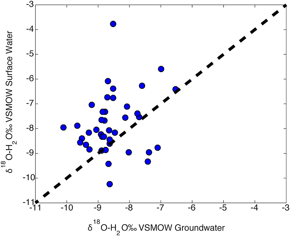
Figure 14. Average surface water, groundwater δ¹⁸O cross plot of samples binned by HUC10 watershed location. Surface waters within the HUC10s tend to be more enriched compared to groundwaters.

Conclusions

Isoscapes and isotopic studies are an important tool to better understand hydroclimatic studies and their effects on water resource and water management. The use of stable isotopes has become a low cost, effective tracer mechanism to gain more knowledge on precipitation dynamics, groundwater recharge mechanisms, paleoclimate, and water resource management (Birkel et al., 2018). A dataset of 1,707 surface water samples, 1,405 groundwater samples, and 558 precipitation samples across Massachusetts has been analyzed in terms of seasonal, temporal, spatial, and environmental variability with the aim of determining and explaining the isotopic signature and variability of precipitation, surface water and groundwater for the state of Massachusetts. A state meteoric water line, surface water line, and groundwater line have been calculated from unweighted precipitation, surface, and groundwater analyses. The SMWL is δ²H = 7.7 δ¹⁸O + 9.8. The SWL is δ²H = 5.7 δ¹⁸O + 4.2, and the GWL is δ²H = 6.6 δ¹⁸O + 4.0, Table 2. SMWL, SWL, and GWL reveal significant differences in slopes and y-intercept, slopes range from 0.9 to 2.0‰. Mean δ¹⁸O and δ²H values of precipitation vary as a function of moisture source, seasonality, elevation and topographic location. Mean δ¹⁸O and δ²H values of surface water vary as a function of open vs. closed water systems, topographic location, seasonality, and precipitation induced seasonality. Mean δ¹⁸O and δ²H values of groundwater vary as a function of hydrogeologic characteristics and topographic location.

TABLE 2

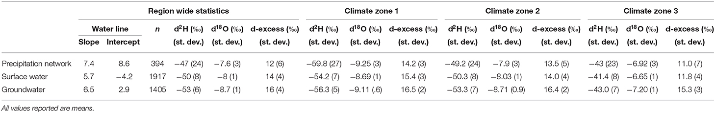
Table 2. Region wide summary statistics of precipitation, surface water, and groundwater and broken down into climate zones.

Spatially, δ¹⁸O and δ²H values for precipitation, surface water, and groundwater illustrate an isotopic separation along an east-west topographic gradient where isotopes are enriched in CZ3, where there is little change in elevation, and depleted in CZ1, where topography varies more. This east to west depletion is primarily due to differences in elevation and relative distance from a moisture source. Median δ¹⁸O values from 2017 and surface water samples 2018 for CZ1, CZ2, and CZ3 were correlated with the median δ¹⁸O values of precipitation. Precipitation median δ¹⁸O values plot consistently higher than both groundwater and surface water datasets. These results imply that the isotopic signature of precipitation gets filtered due to recharge infiltration, evaporation, and evapotranspiration and is reflected in both the surface water and groundwater.

Estimates of young water fractions for surface waters reveal that roughly 40% of total discharge is composed of water that is <2–3 months and that 2.5% of groundwater consists of water that is <2–3 months in age. Correlation between river water data that incorporates monthly precipitation isotopic variation illustrate that roughly 90% of our surface water variability is due to precipitation-evapotranspiration induced seasonality and 9% is due to open water losses. In this paper, we have developed a basic characterization and understanding of the isotopic signatures and variability of precipitation, surface water, and groundwater. We have related the interaction between surface water and groundwater and surface water to precipitation and have determined that a large portion of surface water variability is due to precipitation induced seasonality and groundwater variability reflects the dampening of this seasonality. The good agreement of the spatial patterns in precipitation, surface water, and groundwater will be useful for analyzing the effects of changes in moisture sources and timing and how these changes are propagated through the hydrological cycle in Massachusetts. Furthermore, by relating the surface water to precipitation and surface waters sensitivity to precipitation isotopic variability it will be useful in analyzing the changes in moisture source and how it is reflected in the stable isotope of surface water. This work has the potential to answer many more questions about the hydrologic cycle of Massachusetts and how factors such as catchment size, recharge processes in the vadose zone, and climate change can affect the isotopic topic signature of waters throughout the state of Massachusetts. Further work into studying these factors will improve our basic understanding of the hydrological behavior in a humid post-glacial environment.

Data Availability Statement

The original contributions presented in the study are included in the article/Supplementary Materials, further inquiries can be directed to the corresponding author.

Author Contributions

DB initiated the study, designed and initiated the sample collection, proposed the research questions, secured funding, and led final compilation of manuscript. AC was primarily responsible for data analysis, figure creation, and writing of manuscript. All authors contributed to the article and approved the submitted version.

Conflict of Interest

The authors declare that the research was conducted in the absence of any commercial or financial relationships that could be construed as a potential conflict of interest.

Acknowledgments

We thank support over the years from the Massachusetts Water Resources center for funds through the NIWR USGS 104B program (Grant Number: 2009MA213G). Support from a grant from the Massachusetts Environmental Trust for Grant METFY2018UMAMHERST01 is greatly appreciated.

Supplementary Material

The Supplementary Material for this article can be found online at: https://www.frontiersin.org/articles/10.3389/frwa.2021.645634/full#supplementary-material

References

Akers, P. D., Brook, G. A., Railsback, L. B., Liang, F., Iannon, G., Webster, J. W., et al. (2016). An extended and higher-resolution record of climate and land use from stalagmite MC01 from Macal Chasm, Belize, revealing connections between major dry events, overall climate variability, and Maya sociopolitical changes. Palaeogeogr. Palaeoclimatol. Palaeoecol. 459, 268–288. doi: 10.1016/j.palaeo.2016.07.007

CrossRef Full Text | Google Scholar

Berden, G., Peeters, R., and Meijer, G. (2000). Cavity ring-down spectroscopy: experimental schemes and applications. Int. Rev. Phys. Chem. 19, 565–607. doi: 10.1080/014423500750040627

CrossRef Full Text | Google Scholar

Berry, Z. C., Evaristo, J., Moore, G., Poca, M., Steppe, K., Verrot, L., et al. (2017). The two water worlds hypothesis: addressing multiple working hypotheses and proposing a way forward. Ecohydrology 11:e1843. doi: 10.1002/eco.1843

CrossRef Full Text | Google Scholar

Birkel, C., Helliwell, R., Thornton, B., Gibbs, S., Cooper, P., Soulsby, C., et al. (2018). Characterization of surface water isotope spatial patterns of Scotland. J. Geochem. Explor. 194, 71–80. doi: 10.1016/j.gexplo.2018.07.011

CrossRef Full Text | Google Scholar

Botter, G., Bertuzzo, E., and Rinaldo, A. (2010). Transport in the hydrologic response: travel time distributions, soil moisture dynamics, and the old water paradox. Water Resour. Res. 46, 1–18. doi: 10.1029/2009WR008371

CrossRef Full Text | Google Scholar

Boutt, D. F. (2017). Assessing hydrogeologic controls on dynamic groundwater storage using long-term instrumental records of water table levels. Hydrol. Processes 31:1479. doi: 10.1002/hyp.11119

CrossRef Full Text | Google Scholar

Boutt, D. F., Mabee, S. B., and Yu, Q. (2019). Multiyear increase in the stable isotopic composition of stream water from groundwater recharge due to extreme precipitation. Geophys. Res. Lett. 46, 5323–5330. doi: 10.1029/2019GL082828

CrossRef Full Text | Google Scholar

Bowen, G. (2010). Isoscapes: spatial pattern in isotopic biogeochemistry. Annu. Rev. Earth Planetary Sci. 116, 1–14. doi: 10.1146/annurev-earth-040809-152429

CrossRef Full Text | Google Scholar

Bowen, G., Kennedy, C., Liu, Z., and Stalker, J. (2011). Water balance model for mean annual hydrogen and oxygen isotope distributions in surface waters of the contiguous United States. J. Geophys. Res. 38, 161–187. doi: 10.1029/2010JG001581

CrossRef Full Text | Google Scholar

Bowen, G. J., Ehleringer, J. R., Chesson, L. A., Stange, E., and Cerling, T. E. (2007). Stable isotope ratios of tap water in the contiguous United States. Water Resour. Res. 43:W03419. doi: 10.1029/2006WR005186

CrossRef Full Text | Google Scholar

Brand, W. A., Geilmann, H., Crosson, E. R., and Rella, C. W. (2009). Cavity ring-down spectroscopy versus high-temperature conversion isotope ratio mass spectrometry; a case study on d2H and d18O of pure water samples and alcohol/water mixtures. Rapid Commun. Mass Spectrom. 23, 1879–1884. doi: 10.1002/rcm.4083

CrossRef Full Text | Google Scholar

Celle-Jeanton, H., Gonfiantini, R., Travi, Y., and Sol, B. (2004). Oxygen-18 variations of rainwater during precipitation: application of the Rayleigh model to selected rainfalls in Southern France. J. Hydrol. 289:165–177. doi: 10.1016/j.jhydrol.2003.11.017

CrossRef Full Text | Google Scholar

Cole, A. (2019). Spatial and temporal mapping of distributed precipitation, surface and groundwater stable isotopes enables insights into hydrologic processes operating at a catchment scale (Masters theses). p. 823. Available online at: https://scholarworks.umass.edu/masters_theses_2/823

Google Scholar

Craig, H. (1961). Isotopic variations in meteoric waters. Science 133, 1702–1703. doi: 10.1126/science.133.3465.1702

PubMed Abstract | CrossRef Full Text | Google Scholar

Dansgaard, W. (1964). Stable isotopes in precipitation. Tellus A 16, 436–468. doi: 10.1111/j.2153-3490.1964.tb00181.x

CrossRef Full Text | Google Scholar

Dettinger, M. D., and Diaz, H. F. (2000). Global characteristics of stream flow seasonality and variability. J. Hydrometerol. 1, 289–310. doi: 10.1175/1525-7541(2000)001<0289:GCOSFS>2.0.CO;2

CrossRef Full Text | Google Scholar

Draxler, R. R., and Rolph, G. D. (2003). HYSPLIT (Hybrid Single-Particle Lagrangian Integrated Trajectory) Model Access via NOAA ARL READY Website (http://www.arl.noaa.gov/HYSPLIT.php). College Park, MD: NOAA Air Resources Laboratory.

Google Scholar

Dutton, A., Wilkinson, B. H., Welker, J. M., Bowen, G. J., and Lohmann, K. C. (2005). Spatial Distribution and seasonal variation in 18O/16O of modern precipitation and river water across the conterminous USA. Hydrol. Processes 19, 4121–41446. doi: 10.1002/hyp.5876

CrossRef Full Text | Google Scholar

Earman, S., Campbell, A. R., Phillips, F. M., and Newman, B. D. (2006). Isotopic exchange between snow and atmospheric water vapor: estimation of the snowmelt component of groundwater recharge in southwestern United States. J. Geophys. Res. 111:D09302. doi: 10.1029/2005JD006470

CrossRef Full Text | Google Scholar

Evaristo, J., Jasechko, S., and McDonnell, J. J. (2015). Global separation of plant transpiration from groundwater and streamflow. Nature 525, 91–94. doi: 10.1038/nature14983

PubMed Abstract | CrossRef Full Text | Google Scholar

Gonfiantini, R., Roche, M. A., Olivry, J. C., Fontes, J. C., and Zuppi, G. M. (2001). The altitude effect on the isotopic composition of tropical rains. Elsevier 181, 147–167. doi: 10.1016/S0009-2541(01)00279-0

CrossRef Full Text | Google Scholar

Good, S. P., Noone, D., and Bowen, G. (2015). Hydrologic connectivity constrains partitioning of global terrestrial water fluxes. Science 349, 175–177. doi: 10.1126/science.aaa5931

PubMed Abstract | CrossRef Full Text | Google Scholar

Hervé-Fernández, P., Oyarzún, C., Brumbt, C., Huygens, D., Bodé, S., Verhoest, N. E. C., et al. (2016). Assessing the ‘two water worlds' hypothesis and water sources for native and exotic evergreen species in southcentral Chile. Hydrol. Processes 30, 4227–4241. doi: 10.1002/hyp.10984

CrossRef Full Text | Google Scholar

IAEA (2000). Environmental Isotopes in the Hydrological Cycle: Principles and Applications. Vienna.

Google Scholar

Ingraham, N. L., and Taylor, B. E. (1991). Light stable isotope systematics of large-scale hydrologic regimes in California and Nevada. Water Resour. Res. 27, 77–90. doi: 10.1029/90WR01708

CrossRef Full Text | Google Scholar

Jasechko, S., Birks, S. J., Gleeson, T., Wada, Y., Fawcett, P. J., Sharp, Z. D., et al. (2014). The pronounced seasonality of global groundwater recharge. Water Resour. Res. 50, 8845–8867. doi: 10.1002/2014WR015809

CrossRef Full Text | Google Scholar

Jasechko, S., Wassenaar, L., and Mayer, B. (2017). Isotopic evidence for widespread cold season- biased groundwater recharge and young streamflow across central Canada. Hydrol. Processes 31, 2196–2209. doi: 10.1002/hyp.11175

CrossRef Full Text | Google Scholar

Kendall, C., and Coplen, T. B. (2001). Distribution of oxygen-18 and deuterium in river waters across the United States. Hydrol. Processes 15, 1363–1393. doi: 10.1002/hyp.217

CrossRef Full Text | Google Scholar

Koeniger, P., Gaj, M., Beyer, M., and Himmelsbach, T. (2016). Review on soil water isotope-based groundwater recharge estimations. Hydrol. Processes 30, 2817–2834. doi: 10.1002/hyp.10775

CrossRef Full Text | Google Scholar

Lachniet, M. S., and Patterson, W. P. (2009). Oxygen isotope values of precipitation and surface waters in northern Central America (Belize and Guatemala) are dominated by temperature and amount effects. Earth Planetary Sci. Lett. 284, 435–446. doi: 10.1016/j.epsl.2009.05.010

CrossRef Full Text | Google Scholar

Landais, A., Casado, M., Prié, F., Magand, O., Arnaud, L., Ekaykin, A., et al. (2017). Surface studies of water isotopes in Antarctica for quantitative interpretation of deep ice core data. Comptes Rendus Geosci. 349, 139–150. doi: 10.1016/j.crte.2017.05.003

CrossRef Full Text | Google Scholar

Landwehr, J. M., Coplen, T. B., and Stewart, D. W. (2014). Spatial, seasonal, and source variability in the stable oxygen and hydrogen isotopic composition of tap waters throughout the USA. Hydrol. Processes 28, 5382–5422. doi: 10.1002/hyp.10004

CrossRef Full Text | Google Scholar

Lee, J., Feng, F., Faiia, A., Posmentier, E. S., Kirchner, J. W., Osterhuber, R., et al. (2010). Isotopic evolution of a seasonal snow cover and its melt by isotopic exchange between liquid water and ice. Chem. Geol. 270, 126–134. doi: 10.1016/j.chemgeo.2009.11.011

CrossRef Full Text | Google Scholar

Liu, Z., Bowen, G. J., and Welker, J. M. (2010). Atmospheric circulation is reflected in precipitation isotope gradients over the conterminous United States. J. Geophys. Res. Atmos. 115, 1–14. doi: 10.1029/2010JD014175

CrossRef Full Text | Google Scholar

McGuire, K., and McDonnell, J. (2007). “Stable isotope tracers in watershed hydrology,” in Stable Isotopes in Ecology and Environmental Science, eds Michener, R., and Lajtha, K., (Malden, MA: Blackwell Publishing).

Google Scholar

Mueller Schmied, H., Eisner, S., Franz, D., Wattenbach, M., Portmann, F. T., Flörke, M., et al. (2014). Sensitivity of simulated global-scale freshwater fluxes and storages to input data, hydrological model structure, human water use and calibration. Hydrol. Earth Syst. Sci. 18, 3511–3538. doi: 10.5194/hess-18-3511-2014

CrossRef Full Text | Google Scholar

Olcott, P. G. (1995). Ground Water Atlas of the United States. Connecticut, Maine, Massachusetts, New Hampshire, New York, Rhode Island, Vermont: U.S. Geological Survey Hydrologic Atlas HA−730–M. 1 Map. Available online at: http://pubs.usgs.gov/ha/ha730/ch_m/index.html

Google Scholar

Penna, D., Stenni, B., Šanda, M., Wrede, S., Bogaard, T. A., and Michelini, M. (2012) Technical note: evaluation of between-sample memory effects in the analysis of δ2H δ18O of water samples measured by laser spectroscopes. Hydrol. Earth Syst. Sci. 16, 3925–3933. doi: 10.5194/hess-16-3925-2012.

CrossRef Full Text | Google Scholar

Puntsag, T., Myron, M. J., Campbell, J. L., Klein, E. S., Likens, G. E., Welker, W. M., et al. (2016). Arctic Vortex changes alter the sources and isotopic values of precipitation in northeastern US. Sci. Rep. 6:22647. doi: 10.1038/srep22647

PubMed Abstract | CrossRef Full Text | Google Scholar

Reddy, M. M., Schuster, P., Kendall, C., and Reddy, M. B. (2006). Characterization of surface and ground water d18O seasonal variation and its use for estimating ground water residence times. Hydrol. Process 20, 1753–1772. doi: 10.1002/hyp.5953

CrossRef Full Text | Google Scholar

Ren, W., Yao, T., Xie, S., and You, H. (2016). Controls on the stable isotopes in precipitation and surface waters across the southeastern Tibetan Plateau. J. Hydrol. 545, 276–287. doi: 10.1016/j.jhydrol.2016.12.034

CrossRef Full Text | Google Scholar

Risi, C., Bony, S., Vimeux, F., and Jouzel, J. (2010). Water-stable isotopes in the LMDZ4 general circulation model: model evaluation for present-day and past climates and applications to climatic interpretations of tropical isotopic records. J. Geophys. Res. 115:D24123. doi: 10.1029/2010JD015242

CrossRef Full Text | Google Scholar

Sprenger, M., Leistert, H., Gimbel, K., and Weiler, M. (2016). Illuminating hydrological processes at the soil-vegetation-atmosphere interface with water stable isotopes. Rev. Geophys. 54, 674–704, doi: 10.1002/2015RG000515

CrossRef Full Text | Google Scholar

Sprenger, M., Tetzlaff, D., Buttle, J., Laudon, H., Leistert, H., Mitchell, C. P., et al. (2018). Measuring and modeling stable isotopes of mobile and bulk soil water. Vadose Zone J. 17:170149. doi: 10.2136/vzj2017.08.0149

CrossRef Full Text | Google Scholar

Timsic, S., and Patterson, W. P. (2014). Spatial variability in stable isotope values of surface waters of Eastern Canada and New England. J. Hydrol. 511, 594–604. doi: 10.1016/j.jhydrol.2014.02.017

CrossRef Full Text | Google Scholar

Vachon, R. W., White, J. W. C., Gutmann, E., and Welker, J. M. (2007). Amount-weighted annual isotopic (d18O) values are affected by the seasonality of precipitation: a sensitivity study. Geophys. Res. Lett. 34:L21707. doi: 10.1029/2007GL030547

CrossRef Full Text | Google Scholar

von Freyberg, J., Allen, S. T., Seeger, S., Weiler, M., and Kirchner, J. W. (2018). Sensitivity of young water fractions to hydro-climatic forcing and landscape properties across 22 Swiss catchments. Hydrol. Earth Syst. Sci. 22, 3841–3861. doi: 10.5194/hess-22-3841-2018

CrossRef Full Text | Google Scholar

Wassenaar, L. I., Ahmad, M., Aggarwal, P., van Duren, M., Pöltenstein, L., Araguas, L., et al. (2012). Worldwide proficiency test for routine analysis of d2H and d18O in water by isotope-ratio mass spectrometry and laser absorption spectroscopy. Rapid Commun. Mass Spectrom. 26, 1641–1648. doi: 10.1002/rcm.6270

CrossRef Full Text | Google Scholar

Weider, K., and Boutt, D. (2010). Heterogeneous water table response to climate revealed heterogeneous water table response to climate revealed by 60 years of ground water data. Geophys. Rese. Lett. 37. doi: 10.1029/2010GL045561

CrossRef Full Text | Google Scholar

Welker, J. M. (2000). Isotopic (d18O) characteristics of weekly precipitation collected across the USA: an initial analysis with application to water source studies. Hydrol. Process 14, 1449–1464. doi: 10.1002/1099-1085(20000615)14:8<1449::AID-HYP993>3.0.CO;2-7

CrossRef Full Text | Google Scholar

Welker, J. M. (2012). ENSO effects on δ18O, δ2H and d-excess values in precipitation across the US. using a high-density, long-term network (USNIP). Rapid Commun. Mass Spectrom. 26, 1893–1898. doi: 10.1002/rcm.6298

CrossRef Full Text | Google Scholar

West, A. G., February, E. C., and Bowen, G. J. (2014). Spatial analysis of hydrogen and oxygen stable isotopes (‘isoscape') in groundwater and tap water across South Africa. J. Geochem. Explor. 145:213–222. doi: 10.1016/j.gexplo.2014.06.009

CrossRef Full Text | Google Scholar

Windhorst, D., Waltz, T., Timbe, E., Frede, H. G., and Breuer, L. (2013). Impact of elevation and weather patterns on the isotopic composition of precipitation in a tropical montane rainforest. Hydrol. Earth Syst. Sci. 17, 409–419. doi: 10.5194/hess-17-409-2013

CrossRef Full Text | Google Scholar

Yeh, H. F., Lin, H. I., Lee, C. H., Hsu, K. C., and Wu, C. S. (2014). Identifying seasonal groundwater recharge using environmental stable isotopes. Water 6, 2849–2861. doi: 10.3390/w6102849

CrossRef Full Text | Google Scholar