Statistical Exploration of SENTINEL-1 Data, Terrain Parameters, and in-situ Data for Estimating the Near-Surface Soil Moisture in a Mediterranean Agroecosystem

Schönbrodt-Stitt, Sarah; Ahmadian, Nima; Kurtenbach, Markus; Conrad, Christopher; Romano, Nunzio; Bogena, Heye R.; Vereecken, Harry; Nasta, Paolo

doi:10.3389/frwa.2021.655837

ORIGINAL RESEARCH article

Front. Water, 14 July 2021

Sec. Water and Hydrocomplexity

Volume 3 - 2021 | https://doi.org/10.3389/frwa.2021.655837

Statistical Exploration of SENTINEL-1 Data, Terrain Parameters, and in-situ Data for Estimating the Near-Surface Soil Moisture in a Mediterranean Agroecosystem

$\nSarah Schnbrodt-Stitt$ Sarah Schönbrodt-Stitt¹^*

¹Department of Remote Sensing, Institute of Geography and Geology, University of Würzburg, Würzburg, Germany
²Department of Geoecology, Institute of Geosciences and Geography, University of Halle-Wittenberg, Halle/Saale, Germany
³Department of Agricultural Sciences, Division of Agricultural, Forest and Biosystems Engineering, University of Naples Federico II, Naples, Italy
⁴Agrosphere Institute (Institute of Bio- and Geosciences), Forschungszentrum Jülich, Jülich, Germany

Reliable near-surface soil moisture (θ) information is crucial for supporting risk assessment of future water usage, particularly considering the vulnerability of agroforestry systems of Mediterranean environments to climate change. We propose a simple empirical model by integrating dual-polarimetric Sentinel-1 (S1) Synthetic Aperture Radar (SAR) C-band single-look complex data and topographic information together with in-situ measurements of θ into a random forest (RF) regression approach (10-fold cross-validation). Firstly, we compare two RF models' estimation performances using either 43 SAR parameters ( ${θ_{Nov}}^{SAR}$ ) or the combination of 43 SAR and 10 terrain parameters ( ${θ_{Nov}}^{SAR + Terrain}$ ). Secondly, we analyze the essential parameters in estimating and mapping θ for S1 overpasses twice a day (at 5 a.m. and 5 p.m.) in a high spatiotemporal (17 × 17 m; 6 days) resolution. The developed site-specific calibration-dependent model was tested for a short period in November 2018 in a field-scale agroforestry environment belonging to the “Alento” hydrological observatory in southern Italy. Our results show that the combined SAR + terrain model slightly outperforms the SAR-based model ( ${θ_{Nov}}^{SAR + Terrain}$ with 0.025 and 0.020 m³ m⁻³, and 89% compared to ${θ_{Nov}}^{SAR}$ with 0.028 and 0.022 m³ m⁻³, and 86% in terms of RMSE, MAE, and R²). The higher explanatory power for ${θ_{Nov}}^{SAR + Terrain}$ is assessed with time-variant SAR phase information-dependent elements of the C2 covariance and Kennaugh matrix (i.e., K1, K6, and K1S) and with local (e.g., altitude above channel network) and compound topographic attributes (e.g., wetness index). Our proposed methodological approach constitutes a simple empirical model aiming at estimating θ for rapid surveys with high accuracy. It emphasizes potentials for further improvement (e.g., higher spatiotemporal coverage of ground-truthing) by identifying differences of SAR measurements between S1 overpasses in the morning and afternoon.

Introduction

Globally, experts from diverse applications such as climate, hydrological, and crop yield modeling agree on the importance of the near-surface soil moisture (θ) for improving risk assessment and land and water resources management (Babaeian et al., 2019). It is mainly due to θ acting as a state variable for controlling land-atmosphere feedback and thereby controlling ecosystem dynamics (e.g., Seneviratne et al., 2010; Dorigo et al., 2017).

At the plot to the field-scale, the direct thermo-gravimetric method provides reliable in-situ measurements of θ. Alternatively, indirect methods through the use of portable devices or stationary sensors (e.g., Time Domain Reflectometry) measure the soil dielectric properties from which the soil moisture is inferred through semi-empirical equations (e.g., Rowlandson et al., 2018; Babaeian et al., 2019). However, their applications are rather unfeasible for large-scale operations due to excessive demand for time (e.g., maintenance) and costs (e.g., labor) for surveying (e.g., Santi et al., 2016). Moreover, the significance of ground-based methods is limited to the represented plot settings, and the risk of generating non-representative patterns of θ by spatial regionalization prevails (Chen et al., 2017).

Spaceborne remote sensing (RS) provides spatially explicit information as satellites sense the same ground trace in regular time intervals, allowing for continuous monitoring (Babaeian et al., 2019). Estimates of θ are retrieved from different sensors measuring optical and thermal spectra (e.g., Rahimzadeh-Bajgiran et al., 2013; Zhang and Zhou, 2016), by passive and active microwave sensors (e.g., Schmugge and Jackson, 1997; Das and Paul, 2015), or the synergistic use of different sensor types such as using radar and optical data from Sentinel-2, Landsat, and MODIS (e.g., Attarzadeh et al., 2018; Ayehu et al., 2020; Foucras et al., 2020; Han et al., 2020; Ma et al., 2020). Synthetic Aperture Radars (SAR) are among the most effective and flexible active microwave sensor systems (e.g., Wang and Qu, 2009; Santi et al., 2016) due to their ability to penetrate the near-surface soil layer up to a depth of 5 cm (i.e., for C-band), which in turn enables to observe θ by directly relating the microwave scattering and emission to the water content of the focused object (e.g., Paloscia et al., 2013; Santi et al., 2016; Mohanty et al., 2017; Babaeian et al., 2019).

High spatiotemporal SAR-based retrieval of θ predominantly focusses on bare land surfaces (e.g., Datta et al., 2020), sparsely vegetated areas such as grassland and meadows (e.g., Xu et al., 2020), or agricultural farmland when the vegetation cover is low such as covered by crop residues (e.g., Ayehu et al., 2020). This is mainly due to the unique challenge resulting from the SAR backscatter's high sensitivity to surface characteristics (e.g., roughness) and vegetation properties (e.g., vegetation canopy architecture). From a physical perspective, this is an inherent source of uncertainty in deriving θ (Alemohammad et al., 2019), which can be widely disentangled using backscatter models of different complexity. Numerical theoretical models such as the Integral Equation Model (Baghdadi et al., 2006) and the Kirchhoff Approximation (Gu et al., 2019), and semi-empirical backscatter models such as the Oh model (Oh et al., 1992) and the Water Cloud Model (e.g., Baghdadi et al., 2017) relate the sensor-specific microwave scattering to the target at ground (e.g., bare soil) by means of physical-based descriptions (e.g, Paloscia et al., 2013). They intend to be not site-specific and universally applicable (Paloscia et al., 2013). However, these pyhsical surface scattering models are not valid for vegetation surfaces, hence should not be applied for conditions as present in dense and woody vegetation cover areas (Petropoulos et al., 2015; MirMazloumi and Sahebi, 2016).

The models above mainly require complex radiative transfer algorithmic handling to solve the physical equation systems (e.g., Das and Paul, 2015), thus potentially reducing feasibility for practitioners as stated by Ezzahar et al. (2019). Empirical backscatter models present a simplification by investigating the interaction of microwaves with site-specific surface characteristics but are limited to the area under investigation and require the input of high-quality reference data, e.g., surface roughness (Barrett et al., 2009).

Data-driven machine learning (ML) approaches were investigated for the operational and systematic mapping and monitoring of θ (e.g., Santi et al., 2016; Adeyemi et al., 2018; Cai et al., 2019; Efremova et al., 2019; Datta et al., 2020). Provided the availability of data sufficiently characterizing the system for which θ is to be estimated, they present an adequate alternative (Ezzahar et al., 2019) as they expand the concept of the above backscatter models and allow integration of additional environmental covariates (parameters) beyond those defined for physical modeling.

ML approaches effectively handle large spatial datasets and break down complexity by extracting representative parameters (Karpatne et al., 2019). They can account for the non-linearity of relationships, which is mainly present in RS-based θ retrieval in vegetated and heterogeneous areas (e.g., Chakrabarti et al., 2015). Random forest regression and support vector machine applied on pixels (Hajdu et al., 2018; Datta et al., 2020) or image objects (Ezzahar et al., 2019) and K-Nearest Neighbors for non-parametric regression analysis (Datta et al., 2020) are reported to lead to predictions of increasing accuracy, with even reported less required data compared to mechanistic models (Adeyemi et al., 2018), and enhanced readability of results (Attarzadeh et al., 2018; Ezzahar et al., 2019). ML approaches are increasingly used to estimate θ in agricultural watersheds across humid to arid climate regimes and at different scales (e.g., Quesney et al., 2000; Hachani et al., 2019). They are reported to improve hydrological modeling in wetlands (Dabrowska-Zielinska et al., 2018) and to support the monitoring of water tables dynamics (Asmuß et al., 2019), and the estimation of crop water stress (El-Shirbeny and Abutaleb, 2017), and the water use efficiency (Efremova et al., 2019).

Commonly, studies employ the backscatter intensity Sigma-naught (σ°) either in single (VV or VH) polarization (e.g., Quesney et al., 2000; Attarzadeh et al., 2018; Xu et al., 2020) or dual (VV + VH) polarization (e.g., Dabrowska-Zielinska et al., 2018; Efremova et al., 2019; Datta et al., 2020) from SAR amplitude information only. The topographic effect on radar backscatter, i.e., foreshortening, layover, and shadowing (Chen and Wang, 2008), is considered in the preprocessing of SAR data such as by terrain flattening and orthorectification to remove radiometric distortions (Small, 2011) and to correct distortions induced by the sensor inclination and topography, respectively (Filipponi, 2019). Less attention, however, is paid to the integration of relevant topographic parameters to retrieve spatial patterns of θ in ML approaches.

Contador et al. (2006) applied Artificial Neural Networks for modeling θ based on topography in a Mediterranean watershed in Spain. They stress the strength of topographic variables in predicting area-wide θ as they contribute to explaining spatial information spanning from the very vicinity of a point (e.g., aspect and slope) reflecting the local position to the entire terrain. Notably, compound, topographic attributes such as the contributing area, the flow accumulation, the wetness index, and the topographic roughness allow for integrating the spatial coherence and geographical organization between the different terrain positions (Contador et al., 2006). Subsequently, terrain features enable approximating of spatial patterns θ from an eco-hydrological perspective (e.g., Western et al., 2002; Robinson et al., 2008).

Guevara and Vargas (2019) successfully employed topographic information in an ML approach to downscale RS-based soil moisture products over the conterminous USA and labeled several parameters as “hydrologically meaningful.” In this way, it was possible to adequately address the landscape's capability to physically constrain water inputs (e.g., rain and irrigation water, overland flow) and support the link between spatial variability of soil moisture θ and topography (Guevara and Vargas, 2019).

While the number of studies on Sentinel-1 C-band SAR-based estimation of θ, either by using physical backscatter models or ML approaches, is steadily increasing, and the possibilities for a more accurate analysis under vegetation (e.g., cropland) are explored, application examples from agroforestry sites are not known. This is noteworthy as those sites hold a multifunctional role for a sustainable development model for rural areas (Santoro et al., 2020). Particularly across European Mediterranean regions that is home to one of the global hotspots of agroforestry sites (Gauquelin et al., 2018), they should provide water supply for multiple uses (e.g., domestic water use, irrigation, ecosystem functions) during the dry season (e.g., García-Ruiz et al., 2011). Therefore, θ is crucial for creating scenario-based projections for supporting specific risk assessments (e.g., Nasta et al., 2020).

Our study aims to estimate and map a reasonable short time series of θ in a Mediterranean dry sub-humid, field-scale agroforestry ecosystem in southern Italy using an ML approach. Our objective is to develop a site-specific simplified empirical calibration model that provides the capability to handle SAR backscatters and scarce in-situ information of topsoil θ for a short observation period in November 2018. For calibrating θ from SAR measurements, we aim to employ dual-polarization phase and amplitude information from Sentinel-1 SAR single-look complex (SLC) data to retrieve additional parameters beyond the recent scope of physical and semi-empirical models. To account for the effect of the topography on spatial patterns of θ, we further test the integration of a set of so-called ‘hydrological meaningful’ parameters. For evaluating its estimation performance, we compare the in-situ θ with estimated θ information when building the model (i) with SAR-based parameters only and (ii) with the combination of SAR and terrain parameters. Furthermore, we aim at identifying the most relevant prediction parameters and their temporal behavior (e.g., variability) to enhance understanding of their sensitivity.

Study Area

Our study focuses on a field-scale, predominantly agroforestry area in the headwater zone of the Upper Alento River Catchment in southern Italy (Figure 1; Nasta et al., 2017). It is represented by the rectangular tile (green dashed line) with a size of 1.18 km² in Figure 1A, which comprises the experimental monitoring site MFC2 (Figure 1B) with a size of about 30 ha (drainage divide with an area of 8 ha is represented by the solid blue line; Romano et al., 2018), and its immediate surroundings. The climate is Mediterranean dry sub-humid with hot-dry summer and mild-rainy winter. The average annual rainfall measured at the meteorological station (Figure 1A) amounts to 1,229.3 mm, with 68% (834.9 mm) occurring from October to March. With an average monthly rainfall of 152.2 mm, November is the wettest month (Nasta et al., 2017). The potential evapotranspiration averages 629 mm per year (Nasta et al., 2020).

FIGURE 1

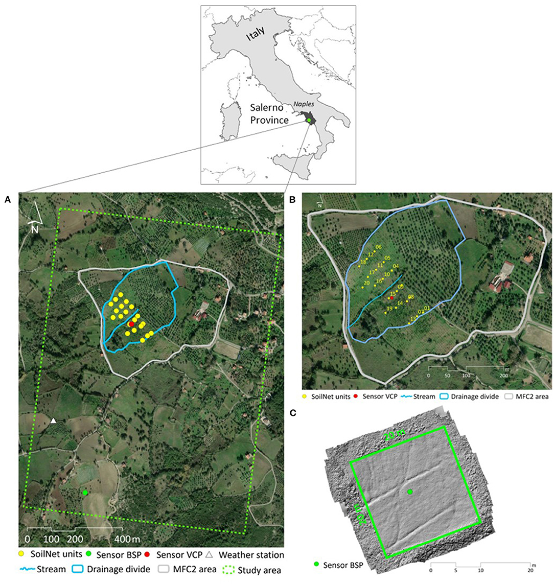
Figure 1. Location of the study area in southern Italy and the soil moisture network. (A) The study area comprises the area of MFC2 with the hydrological divide and the 20 SoilNet units, and the stationary sensor locations VCP in MFC2 and BSP, and the weather station. (B) The area of MFC2 with 20 SoilNet units and the stationary sensor VCP. (C) The bare soil plot with the stationary sensor BSP in its center.

Our in-situ measurements of θ spatially concentrated over 20 designated locations (Figure 1B) that belong to the wireless sensor network (SoilNet; Bogena et al., 2010) installed in the drainage divide of MFC2 in 2016 (Nasta et al., 2020). We further installed two stationary sensors to include the real-field condition in terms of vegetation cover and land-use close (station name VCP; vegetation cover plot represented by the red dot in Figure 1A) and bare soil conditions without any vegetation cover (station name BSP; bare soil plot represented by the green dot in Figure 1A). Later is located about 750 m from the VCP sensor and is represented by a 20 × 20 m square with the stationary sensor located in its center. For the monitoring period, the grass was frequently cut for maintaining the bare soil conditions, as exemplarily shown for March 25, 2019 (Figure 1C) using a hillshade derived from a UAV-based DEM (pixel size ~ 6 mm).

The physical-geographic settings of the moderately steep, south to west facing survey and sensor locations, with mainly silty clayey loam to clayey topsoils (Table 1), reflect the general situation of the study area (Nasta et al., 2019). Vegetation at the 21 observational points within the drainage divide of MFC2 (Figure 1B) is predominantly characterized by the occurrence of cherry (Prunus sp.) and walnut (Juglans sp.) trees growing over a 5 m regular plantation grid with the presence of dense herbaceous vegetation. At the time of investigations (Nov. 2018), all trees showed an indication of progressive abscission. Additionally, olive trees (Olea europaea) with heights between 3 and 5 m grow over a regular plantation grid in proximity to the observational points (Figure 1B). Furthermore, smaller plantations (e.g., olives and vineyards) and agricultural fields allocate in the southern study area (Figure 1A). In Nov. 2018, the majority of those fields lay fallow.

TABLE 1

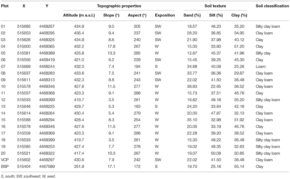
Table 1. Geographical positions (WGS 84/UTM zone 33N), topographic characteristics as derived from a DEM with a cell size of 5 m, and topsoil (0–5 cm) properties of the 20 SoilNet units (01–20) and the stationary sensor locations VCP and BSP.

Materials and Methods

A calibration procedure is necessary to convert SAR-based measurements into θ values at the ground. Therefore, we based our in-situ sampling framework on a measurement sequence per satellite overpasses of Sentinel-1. The constellation of the two polar-orbiting satellites (Sentinel-1 A/B; after this, S1A and S1B) allows for a short revisit time of 6 days over Europe. In Nov. 2018, we organized eight sampling campaigns in four satellite overpass days (c.f., section In-situ Near-Surface Soil Moisture Measurements). Gridded information derived from the S1 SAR products and topographic data (c.f., section Data Processing and Dataset Construction) and in-situ measurements of θ built up the dataset for the spatial estimation of θ (c.f., section Near-Surface Soil Moisture Estimation Using Machine Learning).

In-situ Near-Surface Soil Moisture Measurements

Throughout the observation period, the sampling campaigns were repeatedly conducted over the above exact 20 locations (Figure 1B) to enable fast surveying at the designated and easy-to-recognize flagged locations without using a GPS device. Due to logistic reasons (i.e., darkness during the overpass at 5 a.m.), we set the start and end times of surveying to ~30 min before and after the start and end times of the S1 satellite overpasses (Table 2). We used a portable, low-cost frequency Stevens HydraProbe soil sensor (Stevens Water Monitoring Systems, Inc.) with waveguide lengths of 5.7 cm and inserted it vertically into the topsoil for measuring point-scale θ. The rugged HydraProbe uses the principle of coaxial impedance dielectric reflectometry (Bellingham, 2019) and infers θ in units of water fraction (wfv) with an accuracy of ±0.03 wfv m³ m⁻³ for fine-textured soils and a precision of ±0.003 wfv m³ m⁻³ (Kammerer et al., 2014).

TABLE 2

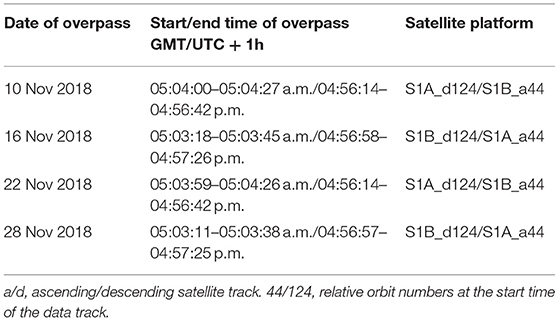
Table 2. Dates with start and end time of overpasses of the satellites Sentinel-1 A/B (S1A/B) during the observation period in Nov. 2018.

At the stationary sensor locations VCP and BSP (Figures 1B,C), further two vertically inserted HydraProbes, each connected to a GeoPrecision datalogger (www.geo-precision.com) and following the exact technical specification as for the portable probe, continuously recorded θ in time-steps of 1 min. We considered those values recorded precisely at the time of satellite overpass (Table 2) for further analyses. Eventually, we compiled a dataset of 176 in-situ measurements (i.e., measurements recorded during eight overpasses at 22 position) of θ according to the proposed calibration procedures.

Data Processing and Dataset Construction

The SAR backscatter that is composed of a pair of symbols denoting the polarization–in our study VV (vertical transmit and vertical receive) and VH (vertical transmit and horizontal receive)–is determined by soil physical properties (e.g., dielectric properties and particle size distribution), topography, and vegetation (plant and canopy structure, vegetation water content). Physical or semi-empirical models attempt to disentangle these properties from the SAR measurements (intensity and phase) that, in turn, are affected by the frequency, polarization, and incidence angle (El Hajj et al., 2018) interacting with the surface properties (Wang and Qu, 2009; Das and Paul, 2015). In our modeling approach, we use such parameters that describe the SAR backscatters and statistically identify the relevant parameters to predict θ.

SAR-Based Parameters

We processed S1A and S1B C-band (5.405 GHz) Level-1 single-look complex (SLC) dual-polarization (dual-pol) SAR data using the Sentinel-1 Toolbox in the Sentinel Application Platform (SNAP). The SAR images were retrieved with a constant and identical Interferometric Wide (IW) sub-swath mode from ascending and descending tracking modes (Table 2). The local incidence angles of the S1A and S1B satellites over our study area vary between near and far range for IW2 mode with values of 36.2–41.9° and 30.6–46.1°, respectively. The look direction (i.e., antenna pointing) for the S1A/B satellites is constantly right, concerning the flight direction. The azimuth steering angle in IW2 mode is ±0.6°.

We first split the swath into desirable sub-swath. Essential preprocessing steps included geocoding of images to add the orbit file with the satellite's exact position and velocity information. Data was radiometrically calibrated to retrieve complex numbers from the digital image pixels and backscattering coefficients (i.e., Beta-naught β°, Sigma-naught σ°, Gamma-naught γ°, and terrain-flattened Gamma-naught TFγ°). The deburst function (Moreira et al., 2013) was applied afterward to remove border noise between the sub-swaths, thus creating continuous images. The polarimetric matrix generation function was used to create the dual-pol covariance matrix, according to Nielsen et al. (2017). Afterward, the multi-looking approach was applied to reducing the speckle noise, thus enhancing the radiometric accuracy, the image quality, and consequently, the interpretability of the SAR image (Moreira et al., 2013). Speckle noise was reduced by applying refined Lee speckle filtering (7 × 7 window) according to Yommy et al. (2015). Due to the topographical effect and the tilt of the satellite sensor, some distortion takes place in SAR images. Therefore, the Range Doppler terrain correction method (Filipponi, 2019) was applied to correct these distortions, and georeferencing was carried out based on (WGS 84, UTM Zone 33N).

The resulting gridded SAR parameters had a spatial resolution of 17 × 17 m and contained both polarizations (cross-pol VH and co-pol VV). To avoid the effects of the different local incidence angles on the backscatter, hence to enable the radiometric comparison of multi-temporal SAR images, all images were normalized to a constant incidence angle of 35° using the quadratic cosine correction based on the theoretical model of Lambert's law and assuming Lambertian surface as typical for moderate vegetation (Mladenova et al., 2013). In addition, we computed mathematical band combinations (MBC) of both polarization in terms of addition (VH+VV), subtraction (VH-VV, VV-VH), ratio (VH/VV, VV/VH), and multiplication (VH^*VV). These MBCs were reported to counteract radiometric instability and vegetation moisture variations introduced by using original polarization (e.g., Omar et al., 2017; Ahmadian et al., 2019) and hence are likely able to improve the performance of our empirical model. The definition of Kennaugh's matrix and its elements for dual-pol S1 data was used based on the calculation by Schmitt et al. (2015) and Ullmann et al. (2017). SVH and SVV refer to the complex signal of cross-pol and co-pol channels, respectively (Table 3). |SVV|² and |SVH|² indicate the intensity of VV and VH channels, whereas Re and Im hold the real and the imaginary part of the inter-channel correlation and * denotes the complex conjugate (Table 3). The Kennaugh elements can be divided into two intensity-only channels K0 and K1, and the two channels K5 and K6 containing the real (Re) and the imaginary (Im) part, respectively (Ullmann et al., 2017). Since the coefficients of the Kennaugh matrix elements for the intensities differ slightly in the literature (e.g., Schmitt et al., 2015; Ullmann et al., 2017), the second version was used according to Schmitt et al. (2015) and is called K0S and K1S, respectively (Table 3).

TABLE 3

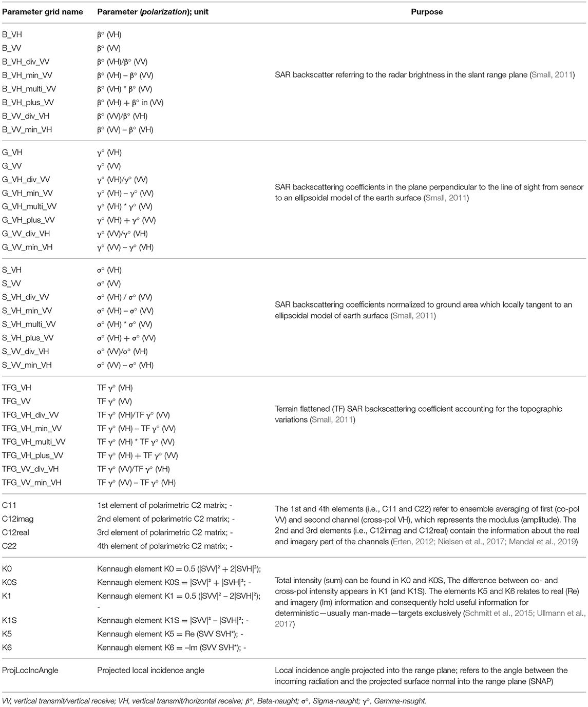
Table 3. List of 43 SAR-based parameters as used as predictors in θ_Nov^SAR and θ_Nov^SAR+Terrain.

Terrain Parameters

We further incorporated continuous, primary local topographic attributes (PLTA) and secondary compound topographic attributes (SCTA) as commonly used environmental proxy-drivers in θ modeling studies (e.g., Western et al., 2002; Beaudette et al., 2013). All attributes were derived using the System for Automated Geoscientific Analyses (Conrad et al., 2015). Due to the predominant processing of SAR parameters, we met the need for the exact cell sizes by re-sampling (i.e., bilinear interpolation) the DEM with an original cell size of 5 m (Nasta et al., 2017) toward the joint spatial resolution of 17 × 17 m. The gridded PLTAs (Table 4) are the altitude above the channel network (AAC), aspect, elevation, slope angle, and plan and profile curvature. Derived SCTAs (Table 4) comprised flow accumulation, SAGA wetness index (SWI), and topographic roughness index (TRI).

TABLE 4

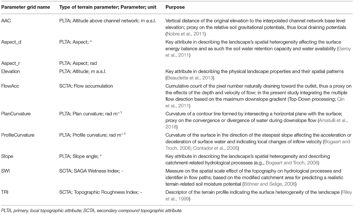
Table 4. Ten terrain parameters as used as predictors in θ_Nov^SAR+Terrain.

In total, we derived 43 SAR and 10 steady-state terrain parameters as spatial gridded datasets. As the SAR measurements are time-variant, they were calculated for each S1 overpass, resulting in 433 single spatial grids.

Near-Surface Soil Moisture Estimation Using Machine Learning

Our ML approach used is the random forests (RF) regression analysis. RF is an ensemble of randomized Classification and Regression Trees (CART), e.g., Breiman (2001). We applied the “caret” R package for regression analysis (Kuhn et al., 2020) for the R Project for Statistical Computing and employed our dataset of 176 in-situ measurements (c.f., section In-situ Near-Surface Soil Moisture Measurements).

The prediction datasets included (i) SAR parameters only (after this ${θ_{Nov}}^{SAR}$ ) and (ii) the combination of SAR and terrain parameters (after this ${θ_{Nov}}^{SAR + Terrain}$ ). Since 70–30% splitting for training/testing did not prove successful because of the limited number of point-observations, we decided for k-fold cross-validation with k = 10, splitting the randomly shuffled data into 10 complementary subsets. From those 10 subsets, nine subsets were used to build and fit the model and one for testing the model. This step was repeated until each subset was used for testing once. The total error rate of the model was then calculated as the average of the individual error rates of the k = 10 individual runs. For both RF models, we kept the tuning parameters ntree (number of trees) and mtry (number of variables randomly sampled at each split) as default values (ntree = 500, mtry = no. of variables/3), which we considered as appropriate as RF is insensitive to over-adaption. We chose the coefficient of determination (R²), the root-mean-square error (RMSE), and the corresponding mean absolute error (MAE) as estimation performance indicators.

Additionally, we computed the predictor importance for ${θ_{Nov}}^{SAR}$ and ${θ_{Nov}}^{SAR + Terrain}$ . It presents the evaluated, scaled relationship between each predictor and the estimates. We used the percentage increase in mean squared error (%IncMSE) as the importance measure for the regression models. It refers to the MSE of predictions, which is calculated by comparing the difference in the influence on model accuracy between a parameter and a randomly permuted version of it at each split in a tree when it is selected (Breiman, 2001). Subsequent importance analysis provides a ranking of predictors and information of how much the model accuracy decreases if we leave out a particular parameter in estimating θ. A one-way ANOVA test was conducted on the averaged values of the topmost ranking parameters as revealed by ${θ_{Nov}}^{SAR}$ to analyze potential differences between the SAR measurements in the morning (5 a.m.) and afternoon (5 p.m.) of each overpass day (Table 2). We assume this step to better identify those parameters sensitive to within-day variations of θ.

Results

In-situ Soil Moisture

In-situ θ values from all eight sampling campaigns (n = 176) spanned from 0.14 m³ m⁻³, measured at position 18 on Nov. 16 (5 a.m.) to ~0.62 m³ m⁻³ at the position BSP on Nov. 22 (5 p.m.). With an average of ~0.34 m³ m⁻³ and a standard deviation (SD) of almost 0.08 m³ m⁻³, the total measured θ values follow a distinct positive, right-tailed distribution (Table 5).

TABLE 5

Table 5. Descriptive statistics of the in-situ soil moisture (m³ m⁻³) over the entire 22 locations at the time of satellite overpasses.

On a daily basis, average in-situ θ values ranged between ~0.30 m³ m⁻³ in the morning (5 a.m.) and afternoon (5 p.m.) of Nov. 16 and ~0.42 m³ m⁻³ (Nov. 22, 5 p.m.; Table 5). The highest θ values (0.48–0.62 m³ m⁻³) were recorded without exception at the sensor location BSP. For all sampling campaigns, θ measured at the BSP location (Figure 1C) was twice as high as at 21 locations within the MFC2 area (Figure 1B). On average, the difference amounts to 140%. For all sampling campaigns, the variation of measured θ values compared to the averages was distinct, with the lowest coefficient of variation (CV) of 12% in the morning of Nov. 28 and the highest CV of 23.2% in the afternoon of Nov. 16 (Table 5). The development of in-situ θ indicated spatiotemporal variations, hence allows us to distinguish between dry and moist situations.

Performance of the RF Models Over the Observational Points

Initial θ estimation of the RF models (c.f., sections Near-Surface Soil Moisture Estimation Using Machine Learning) over the 22 sampling and sensor locations returned very high overall coefficients of determination with R² = 0.86 for ${θ_{Nov}}^{SAR}$ and R² = 0.89 for ${θ_{Nov}}^{SAR + Terrain}$ , even though minor systematic errors in the form of overestimations of low θ (<0.30 m³ m⁻³) were observed in both models (Figure 2). Compared to ${θ_{Nov}}^{SAR}$ , the model ${θ_{Nov}}^{SAR + Terrain}$ can reduce this systematic error slightly. This becomes visible in the corresponding values of RSME = 0.025 m³ m⁻³ and MAE = 0.020 m³ m⁻³ indicating a higher agreement between observed and predicted θ values when including topographic information (Figure 2B).

FIGURE 2

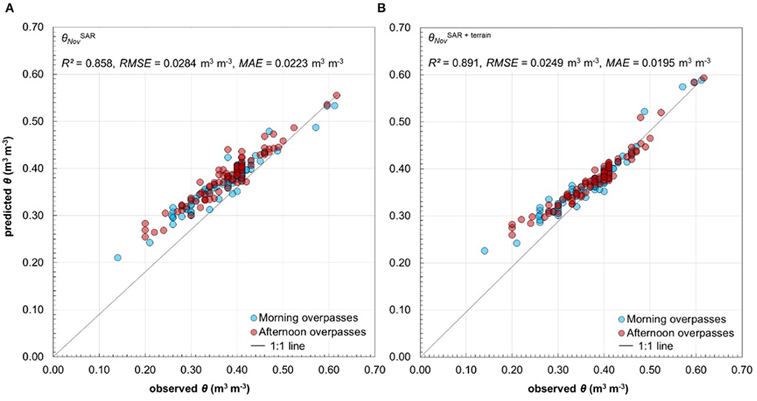
Figure 2. Observed vs. predicted near-surface soil moisture (θ, m³ m⁻³) in Nov. 2018 using the model based on (A) SAR parameters only ( ${θ_{Nov}}^{SAR}$ ) and (B) SAR and terrain parameters combined ( ${θ_{Nov}}^{SAR + Terrain}$ ). The different coloring only serves to visualize the differences between the morning (blue dots) and the afternoon (red dots). The regression models, however, were run over the entirety of the observation points (n = 176).

Additional support in understanding the temporal pattern of θ is gained with the provision of the predictive capability of ${θ_{Nov}}^{SAR}$ and ${θ_{Nov}}^{SAR + Terrain}$ for the single S1 overpasses in the morning (5 a.m.) and in the afternoon (5 p.m.; Figure 3). The model ${θ_{Nov}}^{SAR}$ generally returned high values of R² spanning from 0.71 (Nov. 16, 5 p.m.) to 0.84 (Nov. 22, 5 p.m.). Except for Nov. 16, the explained variances are slightly higher in the afternoon (R² = 0.79 for Nov. 10, R² = 0.84 for Nov. 22) than in the morning (R² = 0.72 for Nov. 10, R² = 0.82 for Nov. 22). For Nov. 28, R² nearly equals for both S1A/B overpasses (R² ~ 0.79 at 5 a.m./5 p.m.). The lowest RMSE values of ~0.023 m³ m⁻³ indicate the highest agreement between observed and estimated at Nov. 10 (5 p.m.) and Nov. 28 (5 a.m.), respectively. In contrast, the lowest agreements (RMSE ~0.034 m³ m⁻³ and ~0.038 m³ m⁻³, respectively) were found for Nov. 16 (Figure 3). The same trend of prediction capability applies for ${θ_{Nov}}^{SAR + Terrain}$ too. Hence, the lowest values of R² were found for Nov. 16 (R² = 0.71 at 5 a.m., R² = 0.69 at 5 p.m.). The highest R² values from ~0.88 to 0.90 were revealed for all other S1 overpasses (Figure 3). Despite for Nov. 16, the incorporation of terrain parameters thus increases the prediction accuracy by the averaged factor of 1.1 and results in a higher agreement between observed and estimated θ (RMSE from 0.016 m³ m⁻³ to 0.021 m³ m⁻³; Figure 3). Again, Nov. 16 remains excluded from this observation.

FIGURE 3

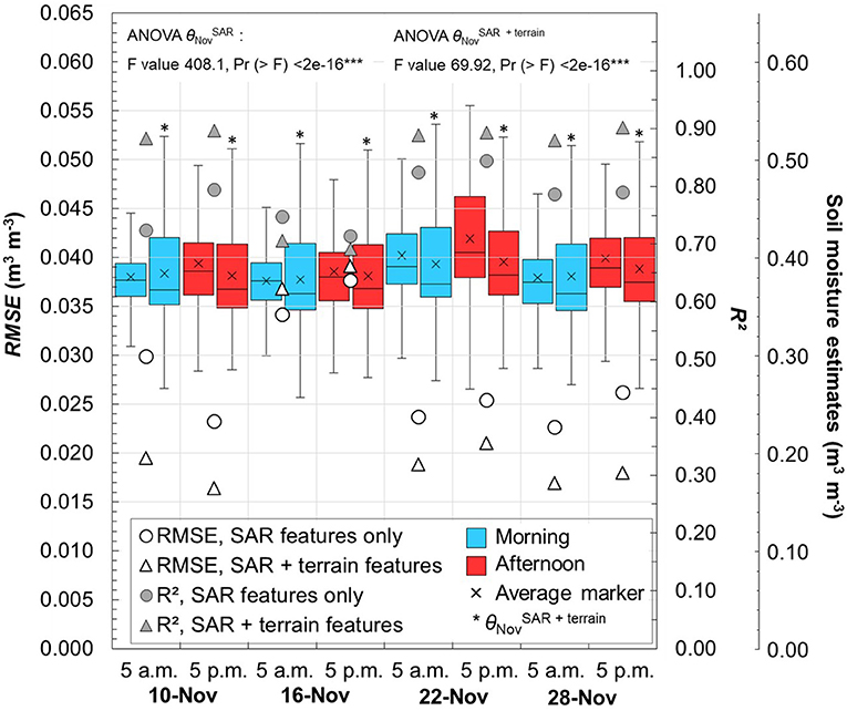
Figure 3. Estimation performance indicators R² (right y axis) and RMSE (left y axis) for the models ${θ_{Nov}}^{SAR}$ and ${θ_{Nov}}^{SAR + Terrain}$ to approximate the in-situ soil moisture (θ) at the eight Sentinel-1 overpasses in Nov. 2018. The box plots show the distributions of the predicted spatial estimates (second y axis at the right) of θ in the morning (blue color) and in the afternoon (red color) for ${θ_{Nov}}^{SAR}$ and ${θ_{Nov}}^{SAR + Terrain}$ (indicated by *).

Time Series of the Near-Surface Soil Moisture

Spatial estimates of θ from ${θ_{Nov}}^{SAR}$ and ${θ_{Nov}}^{SAR + Terrain}$ for the eight S1 overpasses significantly differ with p < 0.001 as revealed by ANOVA testing (Figure 3).

The time series derived from ${θ_{Nov}}^{SAR}$ show distinct, scattered patterns (pixel size of 17 m) of θ. At the beginning of our observation period, the spatial estimates average to 0.380 m³ m⁻³ (CV 9.6%) and 0.394 m³ m⁻³ (CV 12.6%) on Nov. 10 (at 5 a.m. and 5 p.m., respectively). For Nov. 16, the modeling resulted in a slightly lower spatial average of 0.376 m³ m⁻³ (CV 9.7%) on Nov. 16 (at 5 a.m.; Figure 3). Six days later (Nov. 22), spatial patterns of estimated θ change to moist conditions at 5 a.m. (average = 0.402 m³ m⁻³, CV 11.9%) and at 5 p.m. (average = 0.419 m³ m⁻³, CV 13.3%). On Nov. 28, the θ situation nearly returns to that at the start day with similar spatial patterns and average spatial estimates for the morning and afternoon, respectively (Figures 3, 4). The spatial patterns depict a distinct preference of dry and wet pixels so that the area of MFC2 (Figures 1A,B) appears as distinctly drier compared to the very north-eastern and southern part of the study area (Figure 4). The spatial development of θ takes the form of narrow wet bands stretching toward the central study area.

FIGURE 4

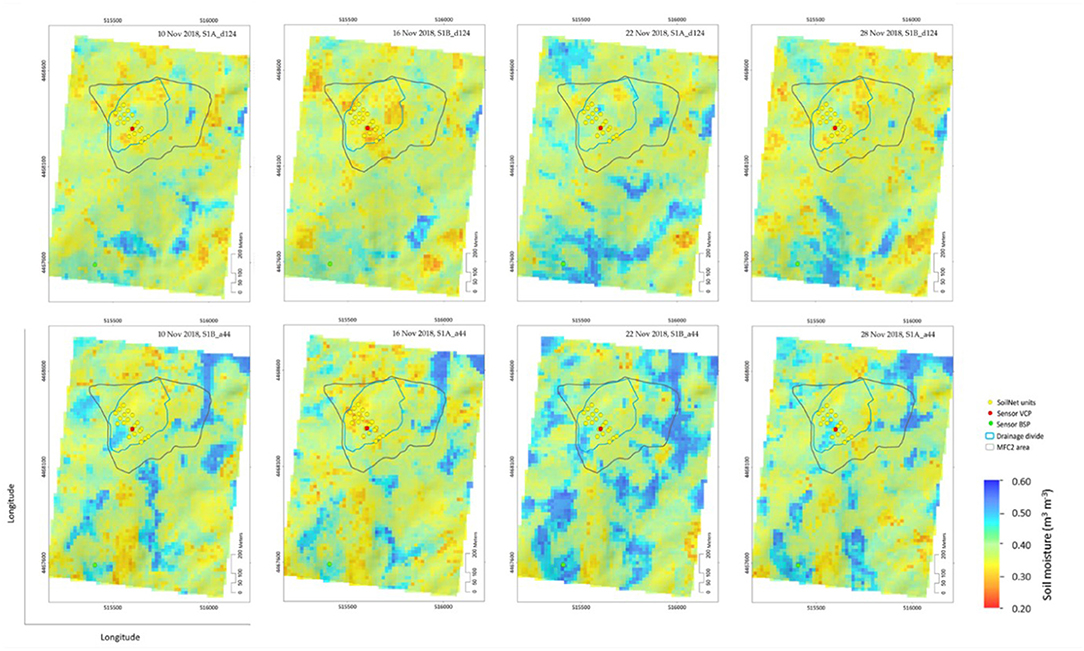
Figure 4. Spatiotemporal patterns of predicted near-surface soil moisture (θ, m³ m⁻³) in the morning (upper row) and in the afternoon based on SAR parameters only ( ${θ_{Nov}}^{SAR}$ ). The pixel size is 17 × 17 m. White pixels refer to no data pixels.

Even though θ estimates obtained from ${θ_{Nov}}^{SAR + Terrain}$ temporally evolve comparable to those from ${θ_{Nov}}^{SAR}$ (Figure 4), the predicted spatial patterns characterize as less scattered but rather smoothed (Figure 5). For the single S1 overpasses, spatial estimates average from 0.377 (Nov. 16, 5 a.m.) to 0.396 m³ m⁻³ (Nov. 22, 5 p.m.) for ${θ_{Nov}}^{SAR + Terrain}$ (Figure 3). The coefficient of variations depicted (CV 12.0% for Nov. 22, 5 p.m. to CV 13.9% for Nov. 28, 5 a.m.) point at slightly higher dispersion of spatial estimates around the average when predicted with ${θ_{Nov}}^{SAR + Terrain}$ as compared to predicting with SAR parameters only (Figure 3).

FIGURE 5

Figure 5. Spatiotemporal patterns of predicted near-surface soil moisture (θ, m³ m⁻³) in the morning (upper row) and in the afternoon (lower row) based on the combination of SAR and terrain parameters ( ${θ_{Nov}}^{SAR + Terrain}$ ). The pixel size is 17 × 17 m. White pixels refer to no data pixels.

Again remarkable is the constantly drier situation in the central study area, represented by the area of MFC2, and supplementing to this, the constantly wetter condition in the southern study area with few very wet spots (~0.51–0.56 m³ m⁻³) surrounding the sensor location BSP (Figure 5). A narrow north-south to the west-east stretching wet band (~0.44–0.48 m³ m⁻³) in the very northern study area constantly occurs throughout the entire time series (Figure 5).

However, the influence of the terrain parameters on the ${θ_{Nov}}^{SAR + Terrain}$ model becomes visible when comparing spatial predictions with that of ${θ_{Nov}}^{SAR}$ (Figures 4, 5). While the θ pattern returned by ${θ_{Nov}}^{SAR + Terrain}$ follows a clear topographical trend and shows the same patterns over the entire period under study, ${θ_{Nov}}^{SAR}$ lacks these constants.

Importance of SAR and Terrain Parameters in Near-Surface Soil Moisture Estimation

The importance of SAR and terrain parameters incorporated in the ensemble models ${θ_{Nov}}^{SAR}$ and ${θ_{Nov}}^{SAR + Terrain}$ (c.f., section Near-Surface Soil Moisture Estimation Using Machine Learning) are sorted decreasingly from top to bottom in Figure 6. For ${θ_{Nov}}^{SAR}$ , the topmost 10 positions (%IncMSE > 47) are predominantly occupied by four out of six Kennaugh elements (K1, K6, K1S, and K0S) and three out of four elements of the C2 matrix (C22, C12imag, and C11). This can be due to information hold by these variables, e.g., the total intensity in K0S and the difference between co-pol and cross-pol intensity in K1. Thus, it is likely that changing the dielectric constant of the target (i.e., soil and vegetation cover) due to the alignment of water dipoles directly affects the intensities and amplitudes (i.e., C11 and C22). The VV co-pol SAR backscatters TFγ° and β°, and the mathematical band combination (MBC) of γ°VV+γ°VH (Table 3) further rank amongst the 10 topmost positions (Figure 6A). Up to position 20 (%IncMSE > 31), mainly MCBs of the SAR backscatters β°, γ°, TFγ°, and σ° either with VH+VV or VH^*VV rank with steadily decreasing parameter importance (Figure 6A). Below ranking position 20 (%IncMSE <30), the VH cross-pol SAR backscatters β°, γ°, and σ°, as well as the remaining 16 MBCs of the SAR backscatters (i.e., VV-VH or VH-VV), and two elements of the C2 (C12real) and Kennaugh (K5) matrix indicate minor prediction importance.

FIGURE 6

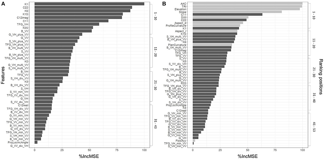
Figure 6. Importance of SAR (dark gray) and terrain (light gray) parameters in the ensemble models built from (A) 43 SAR parameters for ${θ_{Nov}}^{SAR}$ and (B) 53 SAR and terrain parameters for ${θ_{Nov}}^{SAR + Terrain}$ .

The incorporation of terrain parameters into the regression modeling ( ${θ_{Nov}}^{SAR + Terrain}$ ) clearly emphasizes the topography as most crucial in spatially estimating θ (Figure 6B). The 10 topmost ranking positions (%IncMSE > 47) are occupied with seven out of 10 terrain parameters. They mainly characterize as PLTA (i.e., AAC, elevation, slope, aspect in degree, and profile curvature). Among the topmost ranking parameters, the wetness and topographic roughness indices additionally point at the topographic heterogeneity as necessary. Plan curvature (%IncMSE ~38) and flow accumulation (%IncMSE ~4) show moderate to hardly any predictive strength. Among the SAR parameters, the modulus of the polarization channels C11 (%IncMSE ~63) and C22 (%IncMSE ~49) and the Kennaugh element K1 (%IncMSE ~44) are of highest prediction importance in ${θ_{Nov}}^{SAR + Terrain}$ . Below ranking position 10 (%IncMSE <40), further C2 and Kennaugh matrix elements and the SAR backscatters and their MCBs rank in nearly the same order as revealed for ${θ_{Nov}}^{SAR}$ (Figures 6A,B).

Discussion

Spatiotemporal Dynamics of the Near-Surface Soil Moisture

We consider the observed temporal pattern of near-surface soil moisture (θ) to follow the hydrometeorological conditions in the study area. As shown by Nasta et al. (2019), the absence of rainfall and hence, concurrent evapotranspiration losses characterize the first days in November 2018 before starting our observation period and the days between Nov. 10 and Nov. 16. Thus, a likely effect of drying up of θ resulting in a distinct dry spatial pattern in the morning and afternoon of both days is supposed. This can be depicted from both models, the SAR-only-based RF ( ${θ_{Nov}}^{SAR}$ ) and the SAR+terrain-based RF ( ${θ_{Nov}}^{SAR + Terrain}$ ). Two comparatively large rainfall events between Nov. 18 and Nov. 22 amounting to a cumulative rainfall of ~79 mm (Nasta et al., 2019) are discussed to have triggered field wetting with an effect on the spatiotemporal patterns of θ.

When looking at the spatial pattern of the model outputs (Figures 4, 5), an all-time higher spatial θ becomes apparent for the direct surrounding of the sensor location BSP, referring to the bare soil plot (Figure 1C). Compared to the predominantly silty clay loamy and clay loamy topsoil at MFC2 (Table 1), the bare soil plot is the richest in clay (55% clay). Only plot 04 presents a frequently small wet spot in the time series derived from ${θ_{Nov}}^{SAR + Terrain}$ as to be seen from the mapped estimates in the center of the hydrological divide (Figure 5), which is interestingly not apparent from the mapping results when using the SAR parameters as only predictor ensemble (Figure 4). With 51.2%, the clay content at plot 04 is nearly comparable to that at BSP. Specifically, we assume the higher clay content at both positions and the differences in topsoil textures in general (Table 1) to explain the spatial patterns of θ. Numerous studies confirm soils with finer particle sizes (i.e., clay) to retain more soil water, thus influencing the residual water content, independently from short-term changes in rainfall patterns (e.g., Amanabadi et al., 2018; Jiménez-de-Santiago et al., 2019).

Although the time series of θ shows a distinct response to rainfall events (Nasta et al., 2019) and patterns appear plausible, the estimation of θ is, to a certain extent, questionable. Probably, the vegetation is constraining the spatial estimation. The reason might be two-fold. On the one hand, the vegetation considerably governs θ by interception and evaporation, and root water uptake (e.g., Guderle and Hildebrandt, 2015). Yet, this effect cannot be quantified as the survey of such information (i.e., root activity) was considered not feasible in this study. However, we suppose this effect is not distinctly decisive for the present study as Guderle and Hildebrandt (2015) discuss θ data at least from measured recordings to already include information from evapotranspiration and root water uptake patterns. This might be even more relevant as the mainly two-layer vegetation with trees and grass cover (c.f., section Study Area) paused in terms of vegetation activity, and the generally smaller trees at MFC2 were characterized by ongoing abscission at the time of surveying, respectively. However, the vegetation cover poses another uncertainty in our study; The fact that C-band signals are largely influenced by vegetation cover may attenuate the soil contribute to the signal (Quesney et al., 2000). It is also possible that the signals penetrate through vegetation but cannot penetrate the soil as they would do without vegetation.

Additionally, the higher soil moisture content is reported to reduce the penetration depths of the SAR beam (Gorrab et al., 2014). Thus, under- and overestimations in the spatial patterns of θ may be possible, even though the direction of their response to rainfall is considered plausible. The L-band (compared to shorter C-band wavelength) is often recommended to minimize the influence of vegetation on SAR backscattering in estimating θ (e.g., Barrett et al., 2009; El Hajj et al., 2018; Zribi et al., 2019). However, this comes mainly at the cost of data availability and accessibility, data expenses (e.g., Sinha et al., 2015), and the reduced spatial resolution (e.g., Babaeian et al., 2019). Depending on the area of interest and research objective in terms of feasibility, a suitable wavelength must be selected.

Importance of SAR Backscatters and the Topography

We chose our terrain parameters (Table 4) for incorporation into the modeling framework because of their capability to reflect the site-specific soil hydraulic behavior. Therefore, the incorporation of the “hydrologically meaningful” terrain parameters (Guevara and Vargas, 2019) is in line with studies that employed geomorphometry in empirical approaches, such as for downscaling RS-based soil moisture estimates (e.g., Guevara and Vargas, 2019; Mascaro et al., 2019; Zappa et al., 2019). For instance, the SAGA wetness index (SWI) simulates hydrological processes based upon the topography. It is thus capable of reflecting the spatial distribution of soil moisture (Böhner and Selige, 2006), a fact that is regarded as the reasons for the explanatory strength of the SWI in our spatiotemporal modeling of θ (Figure 6A).

Though we did not quantify the effect of the soil as meaningful properties such as texture, organic matter content, bulk density, and hydraulic conductivity (e.g., Jiménez-de-Santiago et al., 2019) were not available as gridded datasets, we ascribe our ${θ_{Nov}}^{SAR + Terrain}$ approach high capability to approximating more realistic patterns of θ compared to ${θ_{Nov}}^{SAR}$ . We mainly assume this to result from the incorporation of “vague proxies” (Behrens and Viscarra Rossel, 2020) in the form of our DEM derivates (Table 4). They are primarly discussed to drive spatial soil property variations and therefore are commonly applied in soil-landscape modeling and digital soil mapping (e.g., Mulder et al., 2011; Zhang et al., 2017). Besides this proxy effect, the topography holds a distinct direct effect; Due to its location in a topographic depression, i.e., characterized by a larger specific contributing area (Qin et al., 2011), the southern-most study area that is represented by the plot location BSP, is found to be generally wetter compared to the higher allocated and less inclined area of MFC2 (Figure 5). Against this background, we assume our choice to incorporate topographic data as crucial baseline information toward the spatial mapping of θ.

In terms of the employed SAR parameters, the intensity-based elements K1, K1S, and K6 and C22, C12imag and C11 from the dual-polarized Kennaugh matrix and covariance matrix, respectively (c.f., section SAR-Based Parameters) were identified most crucial, in both approaches ${θ_{Nov}}^{SARand}$ ${θ_{Nov}}^{SAR + Terrain}$ (Figure 6). To facilitate the discussion of SAR parameters, we tested those topmost important SAR parameters for their temporal significance during the individual S1 satellite overpasses (i.e., at 5 a.m./p.m.) using one-way ANOVA. This is as we assume that they act sensitively to the study area's hydrometeorological conditions (c.f., section Spatiotemporal Dynamics of the Near-Surface Soil Moisture). Figure 7 provides information on their time-variant distributions in the RF model ${θ_{Nov}}^{SAR}$ . Averaged values of the Kennaugh elements K1 and K1S range from 0.009 to 0.012 and from 0.033 to 0.041, respectively. On average, they were measured lowest on Nov. 10 (5 a.m.) and highest on Nov. 22 (5 p.m.). Element K6 was measured lowest (average of −0.001) on Nov. 16 (5 p.m.) and highest (up to an average of 0.001) at 5 a.m. on Nov. 16, 22, and 28. Averaged values of the C2 elements vary from 0.045 to 0.058 (C22), from −0.001 to 0.001 (C12imag), and from 0.012 to 0.017 (C11), respectively. Except for C12imag, the lowest and highest averages were again revealed for Nov. 16, 5 a.m. and Nov. 22, 5 a.m./5 p.m., respectively (Figure 7). We not only observe significant differences (p < 0.001 mainly) in the individual elements between morning and afternoon shots of the same day, except for C11 on Nov. 22 (Figure 7). We also observe a qualitative relationship between those days assigned to drier conditions (Nov. 10 and Nov. 16.) and to wetter conditions (Nov. 22), respectively (c.f., section Spatiotemporal Dynamics of the Near-Surface Soil Moisture).

FIGURE 7

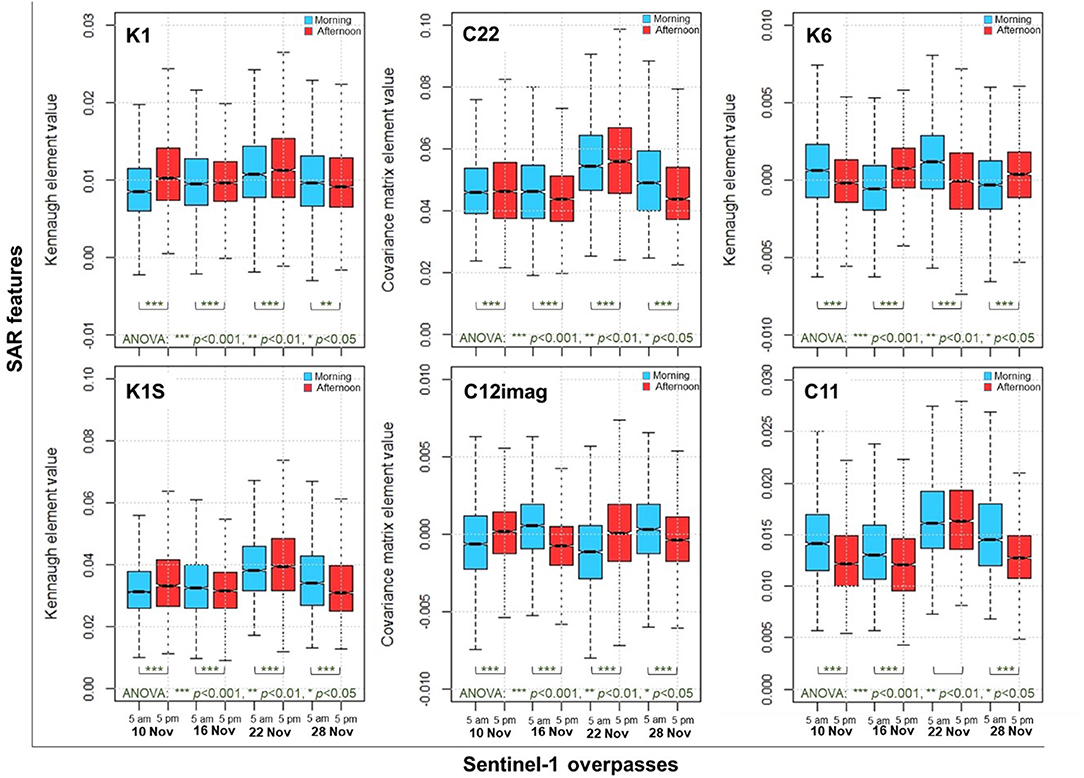
Figure 7. Box plots for the topmost ranking SAR parameters in the RF model θNovSAR for the Sentinel-1 overpasses in the morning (blue color) and in the afternoon (red color). Significant variances of the distributions of parameter values are provided for each day. The asterisks indicate the level of significance (***p < 0.001, **p < 0.01, *p < 0.05). Parameters are displayed according to their order of importance (Figure 6A) from upper left to lower right.

Although empirical models need a significant number of experimental measurements to establish a useful empirical relationship for inversion of soil parameter from backscattering observations (Oh et al., 1992; Walker et al., 2004), and therefore are site-specific and not recommended applicable for monitoring special events or trends beyond the domain of calibration, they are reported to yield accurate results (Wigneron et al., 2003). For this reason, we developed an empirical ML model using an RF 10-fold cross-validation to estimate θ. Even if there is a high correlation between the predictor parameters observed (Table 6), such as between the second versioned Kennaugh elements K0 and K0S (Schmitt et al., 2015), their inclusion was regarded essential to evaluate their effectiveness and importance in terms of their capability for empirically estimating θ. This consideration is supported by Schmitt and Brisco (2013), who state the Kennaugh elements, though derived from dual-co-polarized imaging modes (HH and VV), to distinctly contribute to the robustness and reliability in change detection sufficient for wetland monitoring.

TABLE 6

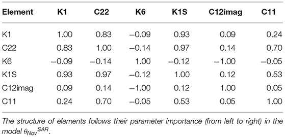
Table 6. Spearman's correlation coefficients ρ (α = 0.05), of the topmost important SAR parameters represented by each three elements of the covariance and Kennaugh matrices.

From Liao et al. (2018), who tested the performance of different polarimetric parameter sets from RADARSAT2 quad-pol data for cropland classification in humid southwestern Ontario, we see that specific elements of the coherency matrix performed best and largely contributed to an overall classification accuracy of 90%. Yet, only a little information is available in such context of θ estimation, with no available information for agroforestry systems in the Mediterranean. Hence, we assume our approach in which we implemented a similar S1 SAR-based predictor set for regression analysis and identified elements of the Kennaugh and covariance matrices to be essential as currently best feasible to retrieving θ in a high spatiotemporal resolution. However, against this background, we aim to omit such highly correlated parameters with respect to their parameter importance in future research to gain optimum parameters.

Transferability and Constraints of the Modeling Framework

Our modeling framework comprises a standardized survey scheme for measuring point-scale θ in accordance with S1 satellite overpasses and RF-based spatial regression analysis to derive a reasonable short time series of θ in November 2018 in a Mediterranean agroforestry environment.

At this point, it should be briefly mentioned that both the measuring instrument (Stevens HydraProbe) and the timing of the field observations in tune with the overpasses of S1 are directly comparable to several recently published studies (Ayehu et al., 2020; Datta et al., 2020; Han et al., 2020; Ma et al., 2020), and thus are regarded as reliable from a technical point of view.

Our framework considers the spatial heterogeneity of the terrain and time-variant backscatter and polarization variables from S1 SLC SAR C-band products (Tables 3, 4) and improves our knowledge of the spatiotemporal dynamics of θ and controlling parameters. Yet, our approach is capable of improvements, most importantly the increase in data availability in terms of higher spatial coverage and a more extended period to optimize the modeling scheme (e.g., testing on unseen data) and to enable more generalized statements, e.g., accurate differentiation of the meteorological forcing (i.e., rainfall) and its response on θ. Of course, this would require more calibration data at the 22 sensor locations considered (Figures 1B,C) and beyond to gather more spatially distributed information. Later is particularly true as zones outside MFC2 show remarkable differences between the SAR-only-based and the SAR+terrain-based RF models and between the SAR measurements for the S1 overpasses in the morning and afternoon. We remind that our empirical calibration models were trained over 22 specific locations at the precise time of eight satellite overpasses for a short observation period of 4 days only. As we trained our site-specific RF model with in-situ data representing the wettest period in the year, we must assume that for the wet-to-dry transition zone, as well as for the dry period and dry-to-wet transition zone (Nasta et al., 2020), it will come up against its limits of what is meaningful. Thus, a final statement on the transferability of the model(s) is only qualitatively feasible at present when considering the same physio-geographic and hydrological settings (e.g., soil texture, slope, vegetation cover) and incidence angle (e.g., Walker et al., 2004). In this context, we consider our approach as best affordable at the given time.

We are aware that both soil moisture and the SAR backscatter are influenced by more factors than addressed in our study. For instance, the soil surface roughness was not considered, although it is reported a major limiting factor for active microwave soil moisture RS (e.g., Sahebi et al., 2002; Schuler et al., 2002; Walker et al., 2004; Wang et al., 2016; El-Shirbeny and Abutaleb, 2017). As no tillage and storm events, commonly known to largely influence the backscatter (e.g., Baghdadi et al., 2008; Dalla Rosa et al., 2012), were notice and recorded, respectively, during our short observation period (i.e., 18 days), we assumed that the surface roughness did not vary and ignored it, particularly as its field survey was considered not feasible.

Furthermore, the occurrence of clouds caught by the close-by mountain ridge (Romano et al., 2018) did not allow for embedding optical (e.g., Sentinel-2) vegetation indices as proxies on the moisture contained in the vegetation and the vegetation activity, such as the leaf area index, the (green) normalized difference vegetation and normalized difference water index, and the fractional vegetation cover (e.g., Attarzadeh et al., 2018; Han et al., 2020; Xu et al., 2020). Here, our model framework offers an open structure toward their gridded integration to account for the potential attenuation of the SAR signal caused by vegetation and enhanced representation of the landscape.

However, we consider our RF approach ( ${θ_{Nov}}^{SAR + Terrain}$ in particular) to compensate for numerous effects and return plausible results despite the neglected factors. This encourages us to continue this kind of empirical assessment by augmenting the in-situ sampling for capturing the entire annual course of hydrometeorological and vegetation conditions. Our achieved results show that although the SAR backscatter is composed of different factors, our site-specific calibration-dependent empirical model is capable of disentangling such effects on the backscatter. Thus, our methodological approach is promising for using and optimizing simplified empirical models over universal and complex physically-based models to spatiotemporally estimate θ. This is particularly encouraging as practitioners might be interested in feasible (e.g., fast surveys for ground-truthing and set-up of predictor sets composed of meaningful parameters) and reliable approaches of high accuracy (Attarzadeh et al., 2018), but at the same time have a limited understanding of the complex theoretical physical properties (Ezzahar et al., 2019).

Conclusions and Outlook

We present a simplified, site-specific calibration model to explore the potentials of Sentinel-1 A/B dual-pol SAR-based phase and amplitude information and in-situ near-surface soil moisture (θ) measured at times of satellite overpasses for the empirical inversion of SAR measurements to gridded estimates of θ. The addition of hydrological meaningful terrain parameters supports capturing the spatial variability of θ by linking the topography at the immediate, surveyed locations to their spatial coherence at the field-scale. We thus not only spatially approximate θ from a technical perspective in terms of physical-numerical interactions of SAR backscatters with surface properties, but rather from a combined approach allowing an eco-hydrological perspective on the spatial patterns of θ. Beyond the predominantly statistical approach, we developed a short-term reasonable time series of θ for a Mediterranean agroforestry ecosystem in southern Italy for November 2018.

Although our proposed model gained high accuracy, we anticipate that its general information value and significance can be enhanced by incorporating more observational data and environmental covariates such as soil (e.g., soil texture and structure) and vegetation properties (e.g., leaf area index and canopy structure), and land use to enable for a more holistic approach. Here, our proposed ML model framework offers an open structure for integrating relevant gridded data. We consider our framework to provide impulses for improvements to address current constraints (i.e., a limited number of in-situ data in space and time). Future research will focus on increasing the number of in-situ observations at times of satellite overpasses over the investigated locations and beyond to optimize the modeling and testing, hence enhancing the mapping accuracy. Subsequently, more robust statements on the spatial heterogeneity and its effect on θ pattern by less over- and underestimations are envisaged. By identifying relevant SAR measurements and topographic information to efficiently parameterize the empirical calibration model to the situation on-site, we attempted to reduce the predictor space toward an optimum of sensitive parameters. The reduction of the computational efforts (e.g., processing time and data storage capacity) is concluded to be of specific relevance for practitioners interested in reliable and feasible approaches to monitoring θ.

Eventually, we consider coupling our model framework and results to hydrological models to support the assessment of surface water fluxes and water balance components, e.g., in groundwater recharge modeling for deriving scenarios of water usage in the Mediterranean agroforestry ecosystems.

Data Availability Statement

The original contributions presented in the study are included in the article/supplementary material, further inquiries can be directed to the corresponding author.

Author Contributions

SS-S, PN, and CC: manuscript design. SS-S: statistical analysis, design of figures and tables, and manuscript editing. PN and NR: regional and hydrological-hydrogeological expertise. MK: in-situ data survey. MK and PN: VCP and BSP sensor maintenance. SS-S, CC, PN, and NR: study design. SS-S, NA, and MK: data processing. HB and HV: provision of SoilNet monitoring infrastructure. All authors contributed to the article and approved the submitted version.

Funding

The Bavarian Research Alliance (grant no. BayIntAn_UWUE_2019_95) and the Italian Ministry of Education, University and Research MiUR (grant no. 2010JHF437) funded the research. The Helmholtz Association and the German Federal Ministry of Education and Research (BMBF) provided funding for the TERENO sensor network infrastructure. Financial support for the maintenance activities was provided by the MiUR-PRIN project. This publication was supported by the Open Access Publication Fund of the University of Würzburg.

Conflict of Interest

The authors declare that the research was conducted in the absence of any commercial or financial relationships that could be construed as a potential conflict of interest.

Acknowledgments

We acknowledge Luigi Giordano from Agriturismo Tre Morene in Monteforte Cilento (Salerno Province) and Benedetto Sica from the University of Naples for supporting the installation of the bare soil plot and for regularly cutting the grass cover.

References

Adeyemi, O., Grove, I., Peets, S., Domun, Y., and Norton, T. (2018). Dynamic neural network modelling of soil moisture content for predictive irrigation scheduling. Sensors 18:3408. doi: 10.3390/s18103408

PubMed Abstract | CrossRef Full Text | Google Scholar

Ahmadian, N., Ullmann, T., Verelst, J., Borg, E., Zöllitz, R., and Conrad, C. (2019). Biomass assessment of agricultural crops using multi-temporal dual-polarimetric TerraSAR-X data. PFG J. Photogramm. Remote Sens. Geoinf. Sci. 87, 159–175. doi: 10.1007/s41064-019-00076-x