 Quentin Chaffaut1*
 Nolwenn Lesparre1
 Frédéric Masson1
 Jacques Hinderer1
 Daniel Viville1Jean-Daniel Bernard1
 Gilbert Ferhat1,2Solenn Cotel1
- 1Université de Strasbourg, CNRS, ENGEES, EOST, ITES UMR7063, Strasbourg, France
- 2Institut National des Sciences Appliquées de Strasbourg, Strasbourg, France
In mountain areas, both the ecosystem and the local population highly depend on water availability. However, water storage dynamics in mountains is challenging to assess because it is highly variable both in time and space. This calls for innovative observation methods that can tackle such measurement challenge. Among them, gravimetry is particularly well-suited as it is directly sensitive–in the sense it does not require any petrophysical relationship–to temporal changes in water content occurring at surface or underground at an intermediate spatial scale (i.e., in a radius of 100 m). To provide constrains on water storage changes in a small headwater catchment (Strengbach catchment, France), we implemented a hybrid gravity approach combining in-situ precise continuous gravity monitoring using a superconducting gravimeter, with relative time-lapse gravity made with a portable Scintrex CG5 gravimeter over a network of 16 stations. This paper presents the resulting spatio-temporal changes in gravity and discusses them in terms of spatial heterogeneities of water storage. We interpret the spatio-temporal changes in gravity by means of: (i) a topography model which assumes spatially homogeneous water storage changes within the catchment, (ii) the topographic wetness index, and (iii) for the first time to our knowledge in a mountain context, by means of a physically based distributed hydrological model. This study therefore demonstrates the ability of hybrid gravimetry to assess the water storage dynamics in a mountain hydrosystem and shows that it provides observations not presumed by the applied physically based distributed hydrological model.
Introduction
Mountain ecosystems provide important water resource locally but also to populations established in the adjacent lowlands (Viviroli et al., 2007). Mountains are also recognized as sentinel for climatic changes as small changes in temperature or precipitation pattern can significantly impact water supply (e.g., Viviroli et al., 2011; Beniston and Stoffel, 2014) or forest ecosystems (Elkin et al., 2013; Beaulieu et al., 2016). This drives the need for new hydrological knowledge and understanding of mountain hydrosystems by integrating more in-situ measurements to complement satellite remote sensing (Bales et al., 2006). In-situ measurements provide access to soil moisture which is a key state variable of hydro-systems, while being challenging to assess because of large variations in space and time at different scales (Vereecken et al., 2014). The development of innovative observation methods allows to tackle this measurement challenge (Bogena et al., 2015). Among them, in-situ time-lapse gravimetry is particularly well-suited for measuring soil water content in mountainous environment as: (i) it is a non-invasive method which does not disturb the hydrosystem in contrast with traditional observation wells, (ii) it is directly sensitive to water content in every compartment of the hydrosystem (surface water, vadose zone and aquifer, e.g., Pfeffer et al., 2013; Champollion et al., 2018, as well as snow and ice, e.g., Voigt et al., 2021) and doesn't require any petrophysical law, and (iii) it is an integrative measurement which is mostly sensitive to changes in water content occurring in a circular area whose radius is ten times the maximal depth of the aquifer, so that for a maximal aquifer depth of 20 m, 90% of the signal comes from <200 m from the station (Leirião et al., 2009; Kennedy et al., 2016). Thus, gravimetry is sensitive to water storage spatio-temporal dynamics–referred as water storage changes (WSC) in the following–at a spatial scale consistent with catchment hydrology. Currently, three types of gravimeters are accurate enough to track the spatiotemporal dynamics of water storage: (i) superconducting gravimeters (Figure 1; Hinderer et al., 2015) provide access to temporal variations in water stock at a fixed position with an accuracy on the order of a few mm of water from minute scale (Delobbe et al., 2019) to multi-year scale (e.g., Creutzfeldt et al., 2012), (ii) ballistic absolute gravimeters such as the FG5 gravimeter (Niebauer et al., 1995) or quantum gravimeters (Ménoret et al., 2018; Cooke et al., 2021) that measure absolute gravity values, on a network of sheltered, vehicle-accessible stations with electrical power (Jacob et al., 2008), (iii) relative field gravimeters such as the Scintrex CG5 (Figure 1; Scintrex Limited, 2012) that allow for the measurement of gravity differences from a reference station and can be deployed on a network of stations with limited access, such as in mountainous areas, which would not be possible with an FG5 absolute gravimeter (e.g., Masson et al., 2012; McClymont et al., 2012; Arnoux et al., 2020). Spatially distributed repeated measurements with relative and absolute field gravimeters provide access to water storage change (WSC) on a seasonal scale with an accuracy on the order of 4 cm of water for FG5 absolute gravimeters (Jacob et al., 2008) and 10 cm of water for Scintrex CG5 relative gravimeters (Gehman et al., 2009; Christiansen et al., 2011).
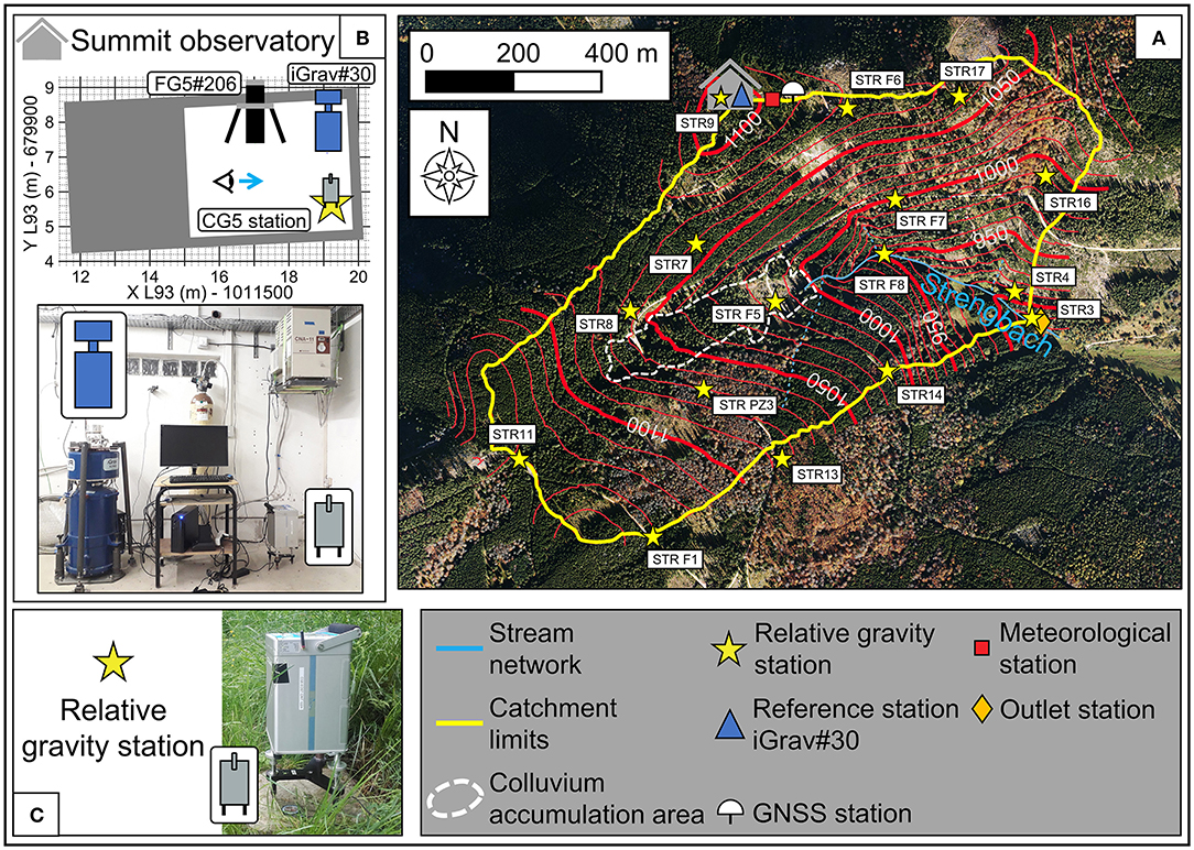
Figure 1. Strengbach catchment hybrid gravity network. (A) Catchment instrumentation map. (B) Organization of the reference gravity station, showing the iGrav#30 SG which serves as gravity reference, and the Scintrex CG5 reference station. (C) A relative gravity station of the microgravimetric network.
Time-lapse gravimetry has been already applied to uncover water storage dynamics in various hydrogeological and climatic contexts. This method was proven successful for assessing WSC in relatively homogeneous to complex alluvial aquifers with confined levels (Pool and Schmidt, 1997; Pool, 2008). Several studies have also shown that gravimetry is a suitable method to monitor water mass redistributions within artificial aquifer recharge sites (Davis et al., 2008; Gehman et al., 2009; Kennedy et al., 2016). Artificial aquifer recharge induces large temporal WSC (i.e., up to several meters of water equivalent), which are on the order of 10 times the accuracy of field gravimeters and are thus easily detectable. However, timelapse gravimetry is also used to characterize the dynamics of hydro-systems with much smaller WSC and/or more complex structure. The method has been successfully applied to karst watersheds in a Mediterranean climate (Jacob et al., 2008, 2010; Champollion et al., 2018), granitic watersheds in West Africa in a tropical monsoon-dominated climate (Christiansen et al., 2011; Pfeffer et al., 2013; Hector et al., 2015), or to a hilly area (Naujoks et al., 2008, 2010). Timelapse gravimetry has been also applied to mountain hydrosystems (Masson et al., 2012; McClymont et al., 2012; Arnoux et al., 2020), though complex to implement because of the poor accessibility of mountain areas. McClymont et al. (2012) conducted a gravity timelapse experiment on a network of 80 stations distributed over a moraine area (1.5 km2) located near a lake collecting meltwater from a Rocky Mountain glacier in Canada. The network was repeated twice at 1-year intervals, once when the lake level was high, and a second time when the lake level was low (i.e., 2 m lower). Only relative gravity measurements were carried out because of the poor accessibility to the studied site did not allow absolute gravity measurements. In order to compensate for the absence of these reference gravity measurements, the authors defined a reference station located outside from the moraine in an area with small WSC, assuming negligible gravity changes at the reference station between the two measurement campaigns. McClymont et al. (2012) measured gravity variations up to 250 nm.s−2 on several stations, which they interpret as the presence of preferential storage areas around these stations. Nevertheless, they admitted that most of the observed gravity variations are in the same order of magnitude as the measurement uncertainties. Arnoux et al. (2020) conducted a similar gravity timelapse on a network of 15 stations on an alpine catchment located in the Swiss Alps. The network was repeated twice within a 3-month interval with a Scintrex CG5. The first acquisition was in summer just after snowmelt in the wet period, and the second acquisition occurred just before the first snow in the dry period. The authors used a station located in the valley bottom as the reference of the relative measurements. Authors could evidence large and significant gravity changes (i.e., up to 1,500 nm.s−2) at stations located on a talus on a topographic flat as well as on a moraine located on steeper slopes, demonstrating the large storage capacity of the talus and the moraine aquifers (i.e., up to 3 m of water). Such media accumulate water during the snowmelt and supply the downstream springs flow during the dry period. Masson et al. (2012) conducted a gravity timelapse experiment on a network of 13 stations on the mid-mountain Strengbach catchment in the French Vosges mountains. The network was repeated 11 times with a Scintrex CG5 between February and June 2011 to monitor the drainage of the Strengbach catchment. To avoid using a potentially singular station as reference station, authors used the mean gravity value of the entire network as reference for each timelapse. With this approach, Masson et al. (2012) could evidence differential gravity changes within the catchment, indicating large water storage decrease around stations located at mid-height of the watershed, and lower water storage decrease for downstream stations.
One can therefore note that in the case of mountain hydrosystems, only relative gravimetric measurements have been carried out, which provides relevant information on differential WSC, but does not allow to infer local absolute WSC around the stations. In addition, the mentioned gravity timelapse experiments do not monitor the entire hydrological cycle, i.e., including the draining and the refilling phases.
As Masson et al. (2012), the present study also targets the Strengbach catchment in the Vosges mountains (France) incorporating the improvement prescribed by Masson et al. (2012): we installed an iGrav superconducting gravimeter (SG) from GWR Instruments Inc (Warburton et al., 2010) in June 2017 at the summit of the catchment (Chaffaut et al., 2020, 2022) to serve as continuous gravity reference. Furthermore, we performed monthly gravity time lapse surveys with a relative field gravimeter (Scintrex CG5) on a network of 16 stations over more than two hydrological cycles from 2018 to 2021. This measurement strategy coupling a monitoring of gravity temporal changes at a reference station with relative gravity time-lapse is referred as hybrid gravimetry (Okubo et al., 2002; Hinderer et al., 2016). We used the SG as local absolute gravity reference for the relative gravity differences measured between station i and the SG station at date t to obtain absolute gravity values at the relative gravity stations:
A great advantage of relative gravity measurement is that every gravity signal common to the full gravity network naturally cancels out, so that is only sensitive to local mass changes and hence mostly to local hydrology. As a result, only the absolute gravity reference needs to be corrected from gravity contributions arising from other causes than local hydrology (see section Reference station).
We applied a distributed physically based hydrological model called NIHM (Normally Integrated Hydrological Model, Weill et al., 2017; Lesparre et al., 2020) to the Strengbach catchment to simulate the coupled surface and underground water flows. NIHM provides as output 3D maps of the subsurface water content at requested times, from which we compute gravity temporal changes at the gravity stations using a 3D forward modeling code. This modeling exercise highlights the supply of observed temporal gravity changes.
The main goal of this study is to show the pertinent contribution of hybrid gravimetry to evidence water storage spatio-temporal dynamics occurring in a small mountain catchment. The paper is organized as follows: In section Studied site we describe the field context. In section Gravimetric data we describe the acquisition and processing of gravity data. In section Measurement results, we present the gravity temporal changes measured over the full observation network, and we show how the acquired gravity data supply an information that is not straightly depicted by gravity changes estimated from the catchment water balance assuming homogeneous water storage changes in the subsurface. So we analyse the scattering of gravity time series potentially related to the relief pattern by computing the topographic wetness index. Finally, we show in section Distributed hydrogravimetric model how the measurements supply unpredicted information by a previously calibrated physically based distributed hydrological model and we discuss the use of hybrid gravity measurements to characterize the water storage spatiotemporal dynamics in mountainous catchments.
Studied Site
The Strengbach Catchment
The Strengbach catchment is a small (i.e., 80 ha) headwater granitic catchment drained by the Strengbach creek and located in the French Vosges mountains (Figure 1). It is part of the OZCAR French network of critical zone observatories (Gaillardet et al., 2018). Catchment climate, hydrology and geochemistry of soil and water are closely monitored by the Observatoire Hydro-Géochimique de l'Environnement (OHGE, http://ohge.unistra.fr; CNRS/University of Strasbourg) since 1986 (Pierret et al., 2018). Climate is temperate of oceanic-mountainous type and forest cover represents 80% of the catchment surface (Figure 1). Topography of the studied area was achieved at a 0.5 m horizontal resolution with a LiDAR survey made in 2011, with horizontal and vertical precision of, respectively, 0.1 and 0.05 m. The catchment altitude ranges from 851 m to 1,151 m, with steep slopes up to 30°. The bedrock consists in fractured granite and a gneiss body along the northern crest, both are covered with a high-porosity saprolite layer of variable thickness, estimated to vary from 1 to 9 m (El Gh'Mari, 1995). Soils are of about 1 m thick with a coarsely grained texture, sandy, and rich in gravel that favors fast infiltration (Fichter et al., 1998; Pierret et al., 2018). As a result, no surface run-off is observed. Then, water flow within the catchment reduces to the river flow and to subsurface flow. The saprolite layer is considered as the main active component of the groundwater flow compartment (Weill et al., 2017; Pierret et al., 2018). Therefore, more deeply connected fractures of the bedrock are assumed to have a negligible contribution to flows joining the river network at the Strengbach catchment scale. In the valley bottom, a saturated area of variable extension is connected to the Strengbach stream (Ladouche et al., 2001).
Water Cycle Monitoring
Overall catchment water storage changes (Figure 2C), referred as CWSC hereafter, results from the balance between: (i) precipitation (bar plot Figure 2B) measured at a 10-min rate at the summit meteorological station (red square, Figure 1), (ii) actual evapotranspiration (green line Figure 2A) modeled at a daily rate using the BILJOU model (Granier et al., 1999) and meteorological data from the summit meteorological station, and (iii) Strengbach stream outflow (see blue line Figure 2A) measured at a 10-min rate (orange diamond, Figure 1). Note that CWSC is a relative quantity of which only the variations have a meaning (Chaffaut et al., 2022). By convention, the minimum of CWSC is set to zero. CWSC exhibits seasonal variations whose yearly range is comprised between 0.20 and 0.25 m for years 2018 and 2019. For the same years, it reached its minimal value at the end of summer, from the end of July to the beginning of October, and its maximal value from January to the end of February, in coincidence with major precipitation events (Chaffaut et al., 2022). The gravity signal is measured at the catchment summit by the superconducting gravimeter iGrav30 (Figure 1B) and results from local water storage dynamics (Chaffaut et al., 2020, 2022; Figure 2D).
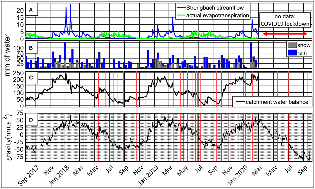
Figure 2. Strengbach catchment hydro-meteorological fluxes together with continuous gravity monitoring at the summit gravity station. (A) Catchment averaged actual evapotranspiration (in green) and Strengbach streamflow (in blue). (B) Catchment averaged precipitations averaged over a 15 days timestep. (C) catchment water storage changes. (D) Temporal gravity changes measured at the summit gravity station. Red lines correspond to the date of the relative gravity surveys.
Hydrogeological Characteristics
A dense Magnetic Resonance Sounding (MRS) measurement campaign has been performed in April-May 2013 and revealed strong heterogeneities of water volume within the Strengbach catchment (Boucher et al., 2015). MRS data inversion revealed a high water volume per unit of area (up to 0,75 m3/m2), referred as specific water volume hereafter, in the flat area upstream the creek main spring and filled by colluvium as well as in the wetland located in the valley bottom. Because of a thinner weathered zone, the specific water volume is lower under the slopes, ranging from intermediate values (i.e., 0.20 to 0.35 m3/m2) in the northern slope to low values (i.e., <0.25 m3/m2) in the southern slopes of the catchment.
More recently, a study combining field observations of pedological, geological and geomorphological features allowed to build a pedological map of the Strengbach catchment that gathered in 8 zones (Figure 8). Lesparre et al. (2020) used this pedological map together with MRS measurements from Boucher et al. (2015) and the flow measured at the catchment outlet to condition a hydrological model, described in section NIHM. This approach allowed to interpret the water volume distribution in terms of subsurface hydrodynamic properties of the active layers made by the soil and the saprolite. As a result, a first spatial distribution of the hydrodynamic parameters in the 8 identified zones has been proposed for the Strengbach catchment (Table 3). Among these zones, the relatively flat colluvium zone upstream the creek main spring (zone 2 Figure 8) and the wetland from Boucher et al. (2015), that corresponds to zone 1 and 3 in Lesparre et al. (2020) and herein (Figure 8) are characterized by large porous volumes per unit area (i.e., from 1.24 to 0.69 m3/m2), referred as specific porous volume hereafter. Other zones located on the slopes or along the crests are characterized by lower specific porous volume (i.e., from 0.52 to 0.12 m3/m2).
As mentioned in the introduction, a first time-lapse microgravity study has been conducted on the Strengbach catchment during the dry spring of 2011 (Masson et al., 2012). The authors showed that the trends of the relative temporal gravity changes were significantly different from one station to the other, meaning that for the 2011 spring period, gravity decreased more, or increased more at some stations than on average. The authors observed a clear spatial consistency of the trend of relative temporal changes and could hence distinguish between 3 groups of stations located in contrasted hydrogeological context: (i) stations located in the valley bottom with flat trends, due to a constant water saturation during the full experiment (ii) stations located on the southern crest with a large gravity increase related to a low water storage capacity (iii) stations with a strong gravity decrease owing to a high water storage capacity at these sites located on the northern part of the catchment and in the colluvium zone.
Gravimetric Data
Hybrid Gravity Network and Relative Gravity Surveys
The gravity network consists in a reference gravity station and a relative gravity network. The reference station is equipped with (i) an absolute station which measured each year with the FG5#206 absolute gravimeter to constrain the SG instrumental drift, (ii) an SG station (blue triangle, Figure 1B) that provides continuous monitoring of gravity changes (Figure 2D), (iii) a relative gravity station (STR9, Figure 1B) used as reference for the relative surveys (Chaffaut et al., 2022).
The relative gravity network consists in 16 relative gravity (RG) stations and is designed to sample hydrologically different areas in the catchment (yellow stars Figure 1A): (i) five stations are located on a crest (STR F1, STR11, STR F6, STR17, and the reference station STR9), (ii) seven stations are located on the slopes (STR13, STR14, STR4, STR7, STR F7, STR16, STR PZ3), (iii) stations STR8 and STR F5 are located in the area filled by colluvium that corresponds to the pedological zone number 2 or at immediate vicinity, (iv) stations STR F8 and STR3 are located nearby the Strengbach creek.
The RG stations correspond to concrete pillars (0.35 × 0.35 × 0.30 m) or to large and stable rocks equipped with a geodetic benchmark. Most of stations have been precisely measured using differential GNSS, using the permanent GNSS station named AUBU (French RENAG network) operating 40 m to the East from the reference station shelter (Figure 1A). Stations that did not provide satisfactory GNSS observing conditions (i.e., trees cover or inside shelter) were observed using a digital level or a total station. The Strengbach catchment zone is not subject to ground uplift or subsidence associated with tectonic activity as shown by the permanent GNSS station (Henrion et al., 2020; Chaffaut et al., 2022), and there is no active landslide on the site. The soil is sandy, so no upward or downward vertical motion of pillars due to soil compaction or expansion induced by clay swelling is expected. In addition, because of the small volume of pillars (0.04 m3), the gravity effect resulting from soil elastic compaction after installing the pillars is likely much lower than 10 nm.s−2, as modeled by Pfeffer (2011). As a result, no significant absolute and/or differential vertical motion should affect the gravity stations.
Our gravity time-lapse monitoring consists in 25 surveys performed between May 2018 and September 2020 with a 1–2 months interval. Unfortunately, it was interrupted from March to May 2020 because of the COVID19 lockdown. Depending on instrument availability, we used the Scintrex CG5 #1224 or #1317 to perform the gravity surveys that were accurately calibrated to integrate both instruments measurement in the same gravity timeseries (see section Calibration of relative gravimeters). We made a strong effort to catch the wettest and the driest states of the hydrosystem with the gravity surveys, as revealed by the CWB and SG residual time series (Figures 2C,D). Wet periods were sampled by a survey in March 2019, and 3 ones in January and February 2020. Dry periods were sampled by 3 surveys in August and September 2018, one survey in September 2019 and a last one September 2020 (Figures 2C,D). The relative gravity network together with the microgravity measurement procedure and gravity data processing is described in Chaffaut et al. (2022).
Reference Station
The SG is installed on the eastern edge of an 8.4 m x 4.4 m shelter with concrete foundations but without gravimetric pillar, while the RG station is installed on the South-East corner, one meter South from SG (Figure 1B). The SG and Scintrex CG5 test masses are located, respectively, 0.23 and 0.27 m above the ground. As both are installed on the edge of the shelter and measuring at a similar height, one can consider that both instruments are measuring the same time-varying gravity signal, so that the SG signal–once appropriately corrected–can serve as absolute gravity reference gRef for the relative gravity measurements (Equation 1). The SG signal contains several time-variable gravity contributions (the tides, the polar motion, the local and continental scale atmospheric signal as well as the local and continental scale hydrology) from which we extract the gravity hydrological residual gRef (Figure 2D). gRefresults from the local hydrology, defined as the water storage spatio-temporal dynamics that occurs within 11 km from the SG. Chaffaut et al. (2020, 2022) provide a full description of the corrections applied on the SG signal to obtain gRef. Corrections are implemented on gRef only as we assume that the contributions not related to the local hydrology are the same for every gravity station of the Strengbach catchment that is of small extent.
gRef exhibits a seasonal cycle ranging from −77 to 74 nm.s−2 (Figure 2D), whose minima occur in August-September in correspondence with the end of the dry summer period, while maxima occur from January to March, in coincidence with major precipitation events falling as snow or rain (Chaffaut et al., 2022). Chaffaut et al. (2022) showed that 72 to 85% of gRef comes from a circular area of 1 km radius centered on the SG. The Strengbach catchment accounts for 25% of this area, while two other neighboring catchments account for the rest of the surface. Therefore, gRef contains an extensive gravity contribution coming from outside of the Strengbach catchment. In the following, the reader has to keep in mind that the absolute gravity signal obtained at each station by combining the gravity reference gRef and the relative gravity measurements Δg (Equation 1) is mainly sensitive to the WSC around each station. results from the water dynamics occurring mainly inside the Strengbach catchment for stations (STR F5, STR PZ3, STR7, STR F7, STR8, STR16, STR F8, STR4). Nevertheless, peripheral stations (i.e., STR F1, STR11, STR9, STR13, STR14, STR F6, STR17 STR3) are more impacted by contributions coming from outside the catchment.
Calibration of Relative Gravimeters
Scintrex CG5 sensors are relative gravimeters that need to be calibrated by comparison with a reference absolute gravimeter. Gravimeters are originally calibrated by the manufacturer (Scintrex Limited, 2012) but calibration needs to be regularly updated because of slight changes in time of the elastic properties of the spring (Cheraghi et al., 2019). The calibration update consists in multiplying gravity simple differences with a corrective calibration factor Cf (Jacob et al., 2010, Equation 2).
is the gravity difference measured by an absolute gravimeter on a calibration line composed of station #1 and #2, while is the gravity difference measured by a CG5 relative gravimeter.
The calibration line we used consists in two gravity stations equipped with SG and maintained by EOST (School and Observatory of Earth Sciences of the University of Strasbourg, https://eost.unistra.fr/en/observatory/geodesy-gravimetry). The first one is located in a buried shelter at the Strasbourg gravity observatory at 180 m of altitude (Longuevergne et al., 2009), while the second one is located at the Strengbach catchment observatory at 1,104 m of altitude (Chaffaut et al., 2020, 2022). Thanks to the important height difference between these stations, the gravity difference reaches as much as 2.13 106 nm.s−2. The calibration line is therefore covering a large gravity range, whose temporal changes (up to 100 nm.s−2, mostly resulting from hydrology) are accurately monitored allowing reliable calibration experiments (Flury et al., 2007). Scintrex CG5 #1224 and #1317 have been calibrated twice in a 2-year long interval to check the stability of sensors bias. The first calibration was made on the 14th of November 2016 (Portier et al., 2018) and the second was made on the 6th of May 2019 (Table 1).
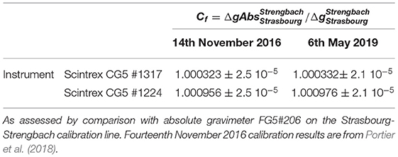
Table 1. Calibration correction factor of Scintrex CG5 #1317 and #1224.
The corrected calibration factor of CG5 #1317 and #1224 did not change significantly between 2016 and 2019 (Table 1). We obtained an accuracy of 2.10−5 (–), which is comparable to the value of 1.10−5 to 2.10−5 (–) reported by Flury et al. (2007). On the Strengbach microgravity network, the largest gravity simple difference reaches 5.105 nm.s−2, so that a change of the calibration factor of 2.10−5 (–) would induce a bias of 10 nm.s−2, which is the reading precision of the Scintrex CG5 gravimeter (Scintrex Limited, 2012). Then, after CG5 measurements have been corrected by applying the Cf coefficient (Equation 2), no significant bias is expected to disrupt the microgravity measurements.
Error Budget
The error time series at station i results from the one standard deviation of the reference gravity value and from the one standard deviation of the gravity difference between station i and the reference station . corresponds to the standard deviation of SG residual time series during the time interval of the relative gravity survey t extending from tStart to tEnd:
ranges between 0.6 and 4 nm.s−2, which is negligible compared to relative gravity measurement error.
is more challenging to assess because it depends on: (i) the instrument performance which is related to e.g., the quality of internal temperature regulation (Jacob et al., 2010; Fores et al., 2016), (ii) on the method used to operate the gravimeter in the field, particularly the loop design (Kennedy and Ferré, 2016) and the handling of the instrument (Repanic and Kuhar, 2018), (iii) on the data selection process and on the method used to compute simple gravity difference. Gravity differences errors are usually computed a-posteriori from observations as the standard deviation of residuals from the least square adjustment of distinct gravity loops (e.g., Flury et al., 2007; Christiansen et al., 2011; Pfeffer et al., 2013; Hector et al., 2015), or by simultaneous adjustment of the full gravity network (e.g., Jacob et al., 2010; McClymont et al., 2012). We refer to this type of error as “formal errors” in the following. In this study, formal errors are considered as a reliable estimate of gravity difference errors (See Annex A and Figure 1C).
Both and errors are assumed to be independent so:
Once correctly calibrated, simple differences obtained from CG5 measurements are considered as bias free.
Median error (i.e., the median of the error time series as defined by equation 4) on hybrid gravity measurements ranges from 20 nm.s−2 for STR8 to 60 nm.s−2 for STR F1 (Figure 3; Table 2). Stations with small median error (<30 nm.s−2) correspond to stations that benefited from redundant measurements during surveys. On the contrary, stations with (relatively) large median error (>50 nm.s−2) were less repeated as they are far from the reference station and/or poorly. As a result, the implemented gravity monitoring campaign should allow to detect gravity temporal changes that are twice the error bar level, which corresponds to 40 nm.s−2 for station STR8 and to 120 nm.s−2 for station STRF1.

Figure 3. Hybrid gravity error distribution by station. The lower and upper end of the whisker, respectively, indicates the minimum and maximum error, the lower and higher blue line corresponds, respectively, to the first and the third quartile, the red line corresponds to the median error, and the red crosses correspond to outliers.
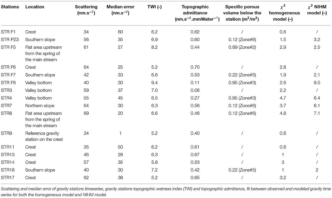
Table 2. Characteristics of observed and modeled gravity time series.
Measurement Results
Gravity Time Series
Gravity time series of stations located in the vicinity of the crest or along the slope are respectively presented in Figures 4A–C. Results for stations located in the valley bottom or nearby the spring of the main creek are presented in Figure 4D.
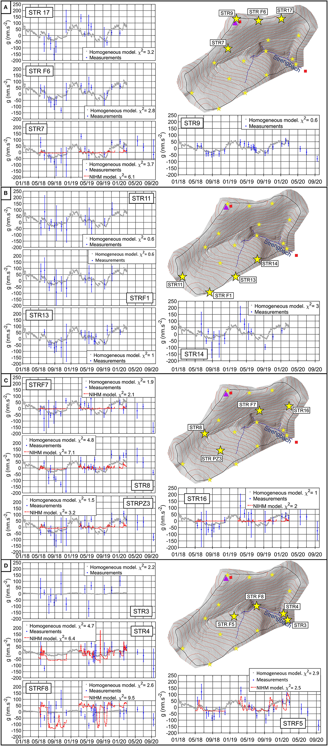
Figure 4. Observed and modeled gravity temporal changes on the gravity stations network. (A,B) Time series of stations located in the vicinity of the catchment boundaries. (C) Time series of stations located along the slope. (D) Time series of stations located in the valley bottom or nearby the spring of the Strengbach creek.
Stations STR F5, STR14, STR F6, STR13, STR8, and STR9 exhibit a seasonal temporal pattern (Figure 4) with maximal gravity values in May 2018, March 2019, and end of February 2020, when catchment water storageis high, as assessed from catchment WSC (i.e., from 150 to 250 mm of water, Figure 2C). For those stations, the gravity signal gradually decreases to a minimum in September 2018, 2019, and 2020 when catchment storage is low (i.e., from 0 to 50 mm of water, Figure 2C). Among these stations, STR F5 exhibits little inter-annual variability as it shows a similar range of gravity changes for the 2019 and 2020 discharge periods (respectively, 219 ± 45 and 233 ± 46 nm.s−2). On the contrary, STR8 exhibits a significant inter-annual variability with a gravity decreases by 129 ± 22 nm.s−2 between the 14 of June and the 11 of September in 2018, a similar decrease of 149 ± 36 nm.s−2 between the 24 of February and the 16 of September in 2020, while in the gravity decreases by only 64 ± 33 nm.s−2 between the 19 of March and the 11 of September in 2019. Other stations are characterized by (i) more complex temporal changes as STR F8, STR4, and STR3 or (ii) temporal changes of lower amplitude with lower signal to noise ratio as for stations STR11 or STR F1. For comparing the gravity signals measured at the different stations, we use the gravity time series scattering σ as indicator of stations time variability. We define σi as the error weighted standard deviation of the gravity time series of station i:
where N is the number of measurements, and is a ponderation factor that corresponds to the inverse of the measurement error (as defined by Equation 4).
There are strong contrasts of σ between stations, revealing spatially heterogeneous gravity temporal changes (Figure 5). The STR8, STR F5, STR7, STR17, and STR F6 stations are characterized by high σ (>62 nm.s−2), while stations STR9, STR11, STR F1, STR F8, STR F7, and STR13 have low σ (<46 nm.s−2). Stations with low σ (i.e., low temporal variability) correspond to areas with low WSC and/or areas with low topographic amplification (see section Homogeneous WSC distribution), while stations with high σ (i.e., high temporal variability) correspond to areas with high WSC and/or areas with high topographic amplification. Note that due to its location in the reference station shelter (Figure 1B), station STR9 is subject to the umbrella effect, which likely explains the low σ. The shelter acts as an umbrella which prevents water infiltration below the gravimeter and consequently reduces WSC occurring in the close surrounding of the gravity sensor (Creutzfeldt et al., 2008; Deville et al., 2013; Reich et al., 2019). These hypotheses are tested in sections Homogeneous WSC distribution, Variability of gravity timeseries in light of Topographic wetness index estimates, and Distributed hydrogravimetric model, where we model gravity changes from WSC assuming different spatial distributions for WSC and compare them with observed gravity changes.
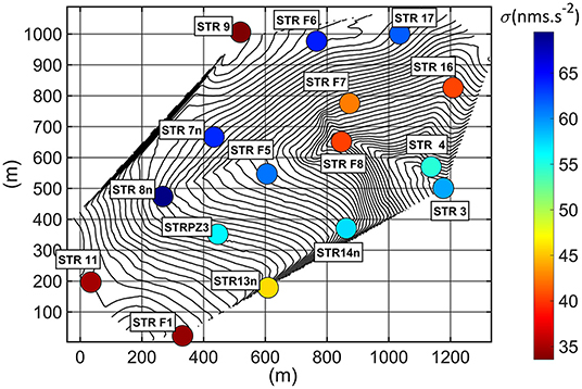
Figure 5. Observed gravity time series scattering. Time series scattering σ is computed using Equation 5.
Homogeneous WSC Distribution
As already pointed by Masson et al. (2012) and Halloran (2021), the topography modulates the gravimetric effect of water storage changes, so that even spatially homogeneous WSC produces spatially heterogeneous gravity changes. In order to investigate this topography effect, we modeled the gravity changes resulting from spatially homogeneous WSC distributed over the topography. For this purpose, we computed the topographic admittance map, where the topographic admittance corresponds to the conversion factor between gravity changes and WSC assumed to be spatially homogeneous.
The topographic admittance Atopo is defined as the gravity effect of a 1 mm thick water layer draped on the topography (Figure 6B). For that, we assume that Atopo corresponds to the gravity effect of a 0.1 m thick layer with a volumetric mass of 10 kg.m−3 (i.e., which is equivalent to a 1 mm thick water layer) whose top follow the topography. We compute the topographic admittance, using the method developed by Leirião et al. (2009) and applied in Chaffaut et al. (2020, 2022), for virtual gravity stations distributed over the Strengbach catchment with a spacing of 6 m between each station. The gravity signal is higher on the ridges with values >0.7 nm.s−2.mmWater−1 compared to the classical Bouguer value of 0.42 nm.s−2.mmWater−1 for a flat terrain (red area Figure 6A). In such regions, the water layer induces a downward gravitational attraction added to the standard gravity field. On the contrary, in the valley bottom, the water layer induces a decrease of the gravity <0.2 nm.s−2.mmWater−1 compared to the Bouguer value (blue area Figure 6A). As a result, one can expect a higher gravity signal for stations located on the crest such as STR F1, STR11, STR F6, and STR17, with admittance values ranging >0.6 (Table 2). The topography also leads to a low gravity signal at stations located in the valley bottom as STR3, STR4, and STR F8, with admittance values <0.27 nm.s−2.mmWater− (Table 2). Note that despite its summit location, the station STR9 has a rather low topographic admittance of 0.40 nm.s−2.mmWater−1 as a result of the mentioned umbrella effect.
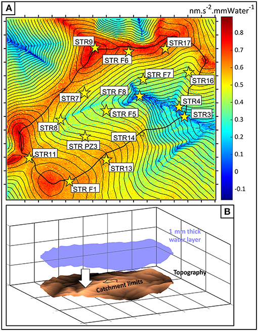
Figure 6. Hydro-gravimetric modeling assuming spatially homogeneous water storage changes. (A) Topographic admittance map i.e., gravity effect due to of a uniform layer of 1 mm of water draped over the topography. (B) Schematic view showing the water body used to compute the topographic admittance map.
Assuming that water storage changes are spatially homogeneous, one can directly compute temporal gravity changes at station i as the product of the catchment water storage changes CWSC (Figure 2C) and the topographic admittance at station i:
We compute as an error weighted misfit value to evaluate the discrepancy between measured gravity changes and modeled gravity changes . Best fits should have χ2 close to 1, indicating that differences between measured and modeled gravity changes are close from the measurement error (defined by Equation 4):
For stations STR F1, STR F7, STR11, STR9, STR13 STR16, and STR PZ3 χ2 ≤ 1.9 (Table 2; Figure 4), so that for these stations, measured and modeled gravity changes does not differ significantly from each other as both exhibit a seasonal cycle (with higher values during the wetter period) of similar range. Hence, gravity temporal changes observed at these stations can be explained by spatially homogeneous catchment water storage changes. Other stations are characterized by higher values with 2.2 ≤ χ2 ≤ 4.8 for stations STR3, STRF8, STRF6, STRF5, STR14, STR17, STR7, STR4, and STR8. At such stations, the observed gravity changes indicate that local WSC differ from catchment averaged WSC. For stations STR F5, STR7, and STR14, and to a lesser extent for stations STR F6 and STR 17, although both observed and modeled gravity changes exhibit a similar seasonal pattern, observed gravity changes have significantly larger ranges indicating WSC of larger amplitude around these stations compared to the catchment averaged WSC. For station STR F5, the observed gravity range is >200 nm.s−2 for the May-September 2018 and March–September 2019 periods, while the range of modeled gravity estimated at the same dates is ≤ 44 nm.s−2 (Figure 4). Observed Gravity changes suggest that in the surrounding of STR F5, WSC range is at least 5 times higher than the catchment averaged WSC, i.e., ≥0.5 m of water. For station STR7, the observed gravity range is >140 nm.s−2 for the May-September and March-September 2019 periods, while modeled gravity range is, respectively, ≤ 57 nm.s−2 (Figure 4). For station STR14, observed gravity range is 248 ± 63 nm.s−2 for the March-September 2019 period, while modeled gravity range is 54 nm.s−2 (Figure 4). For station STR8, observed gravity range is 129 ± 28 nm.s−2 for the May–September 2018 period and observed gravity continues to decrease until the end of November 2018, while modeled gravity stops decreasing in September 2018 and it's range is only 39 nm.s−2 (Figure 4). For the March-September 2019 period and in contrast with the 2018 period, STR8 observed gravity exhibits a much smaller range of 71 ± 36 nm.s−2 which is similar to the modeled gravity range of 45 nm.s−2.
For stations STR3, STR4, and STR F8 that are located in the valley bottom, observed and modeled gravity significantly differ from each other, both in term of temporal patterns and ranges, indicating that these stations exhibit complex WSC in their surrounding that cannot be modeled with this single topographic admittance approach.
Thus, the topography effect alone cannot explain the observed spatio-temporal gravity changes, so spatially heterogeneous WSC conspicuously occur within the catchment, in the sense that local WSC differ from catchment averaged WSC for at least 10 of the 16 stations of the gravity network. Note that because of the low sensitivity of gravimetry to the depth at which WSC occur, we would have obtain very similar results when computing the topographic admittance assuming a different vertical distribution for water, e.g., by considering a 0.1 m thick layer with the same volumetric mass but located at 1 m of depth, or by considering a 1 m thick layer with a volumetric mass of 1 kg.m−3 located between the ground surface and 1 m of depth. We now have to identify the hydrological processes that lead to the spatially heterogeneous WSC we inferred from the comparison between the homogeneous model and the gravity observations.
Variability of Gravity Timeseries in Light of Topographic Wetness Index Estimates
We use the topographic wetness index (TWI), to evaluate the role of the topography on the flows in the Strengbach catchment and to identify preferential storage areas that could explain the large WSC inferred from the gravity observations around stations STR F5, STR8, or STR14. TWI is defined as , where α is the surface of the upslope draining area and tan(β) the local slope (Beven and Kirkby, 1979). The TWI relies on the assumption that the local slope is an adequate proxy for the effective downslope hydraulic gradient, which is very likely for the Strengbach catchment because it is characterized by steep slopes, so that other factors like subsurface spatial heterogeneities might exert a second-order control on the hydraulic gradient (Weill et al., 2017). TWI is a widely used indicator to assess the topographic control on the spatial pattern of saturated area (Grabs et al., 2009) or groundwater depth and soil wetness (Sørensen et al., 2006). Mouyen et al. (2012) also found a correlation between TWI and gravity changes caused by a strong typhoon in Taiwan.
The TWI is used here as a proxy of water storage potential within the Strengbach catchment in relation with the relief pattern (Figure 7A). High TWI values might be related to areas with high water storage potential as valley bottom (with low slopes and large upslope draining area) while low TWI values might indicate areas with low water storage potential as crests (with steep slopes and small upslope draining area). The average TWI is computed from the topography within disks of 20 m radius centered on gravity stations.
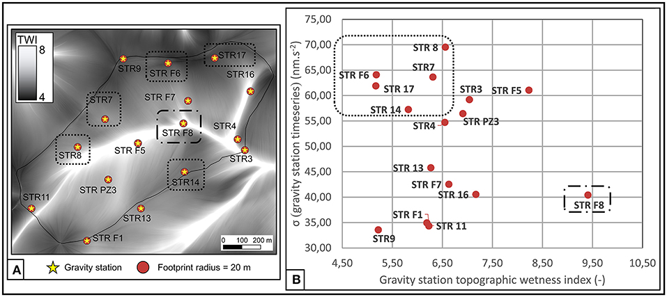
Figure 7. Comparison between topographic wetness index (TWI) and gravity time series scattering. (A) TWI map. (B) Gravity time series scattering vs. TWI.
STR F5 and STR F8 have the largest TWI values >=8.2 because of the small local slope and the large upslope draining area of both stations. STR F5 is located inside a flat area which collects water from the northern and southern slopes, while STR F8 is located in the narrow valley bottom at a crossing point between the Strengbach stream (Figure 8A). Stations located on the slopes exhibit intermediate TWI values while those located on the upper crest line exhibit the lowest TWI values ranging from ≤ 6.2 (Table 2).
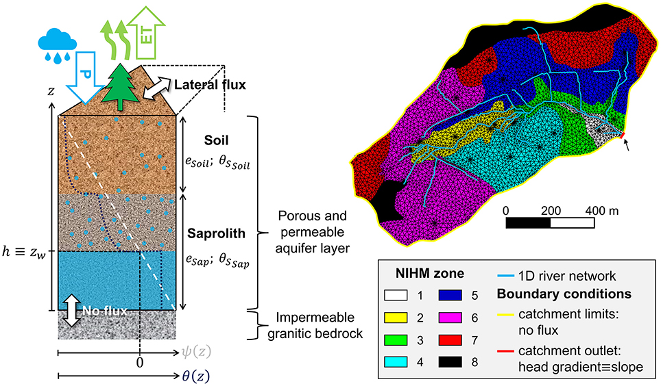
Figure 8. Schematic diagram of the NIHM hydrological model. Left: vertical view showing the vertical parameterization of the NIHM model and the water content distribution in a cell, zw referring to the aquifer level. Right: Horizontal view showing the parametrization of NIHM in 8 hydrological zones.
For each station, we compare the gravity time series σ (Equation 5) to the average TWI (Figure 7B) and distinguish four categories of stations: (i) station F8 with the highest TWI of 9.4 and a low tσ =40 nm.s−2, (rectangle with large dashes Figure 7B) (ii) stations STR F6, STR8, STR7, STR17, STR14 with low TWI (< 6.6) and high σ > 57 nm.s−2 (rectangle with small dashes Figure 7B). For other stations there is a positive correlation between the TWI and σ, so we distinguish two other categories: (iii) stations STR4, STR PZ3, STR3, and STR F5 with a relatively high TWI >6.55 and high σ >55 nm.s−2, iv) stations STR9, STR F1, STR11, STR13, STR F7, STR16 with a relatively low TWI < 7.2 and low σ < 46 nm.s−2.
For stations of the iii and iv categories, TWI shows a linear relationship with σ (Figure 7B), and hence provides clues on the hydrogeological characteristics around these sites. Stations STR F1, STR11, STR13, STR F7, and STR16 are characterized by low TWI and σ values despite relatively large admittance values (Figure 7B; Table 2). So for such stations, water flow related to the topography compensate the relief amplification effect. These sites are characterized by low seasonal water storage changes, which is consistent with the low water storage proposed by Masson et al. (2012). The small storage capacity under such stations can be related to the stations position on the southern crest, by the small upstream draining area or by the steep slope beneath the stations. MRS also evidenced the low amount of stored water around such sites (Boucher et al., 2015; Lesparre et al., 2020).
Stations STR3, STR4, STRPZ3, and STRF5 are characterized by high TWI and σ values (Figure 7B). The local topography around such stations favors water storage and gravity measurements confirm the underground storage capacity enabling the observed temporal WSC. MRS measurement also show a relatively high water content close to STRF5 (Boucher et al., 2015) located in the colluvium zone on a small slope and with a large upstream draining area. Interestingly, such large water storage changes have been already proposed by Masson et al. (2012) to explain the large gravity changes observed at the STR15 station (not monitored here) located inside this zone.
The low σ of STR F8 associated to a high TWI value likely results from the fact that it is located in a saturated area (Ladouche et al., 2001). This implies limited water storage changes across the hydrological cycle and hence leads to small absolute gravity changes, as proposed by Masson et al. (2012) for the station STR5 (not monitored in our study), located 50 m downstream from STR F8.
Stations STR F6, STR17, STR7, STR8, and STR14 are characterized by gravity changes of large amplitude (Figures 4, 5; Table 2), already pointed by Masson et al. (2012) for stations STR14 and STR8. We could not explain these observations by the topography amplification effect nor by relatively low TWI (Table 2) due to a small draining area and/or a high local slope. Preferential water storage might thus occur around these sites, possibly because of a low hydraulic conductivity downstream and/or a relatively large porous space to store water. Indeed, the station STR F6 is located nearby a gneiss body on the northern crest with a clay-rich weathered zone (Boucher et al., 2015; Pierret et al., 2018), which could favor water storage by preventing efficient draining of water. Furthermore, this station is also located nearby a pond and an intermittent spring at the granite-gneiss interface which usually flows until June-July that indicates water storage in the Gneiss body of the northern crest.
Distributed Hydrogravimetric Model
NIHM
For modeling the water storage dynamics in the Strengbach catchment we use the Normally Integrated Hydrological Model (NIHM), which is a low dimensional distributed and physically based hydrological model that couples surface and subsurface flows (Weill et al., 2017; Jeannot et al., 2018). Surface flow is handled with a 1D river model that describes runoff in a ramified stream network (blue lines, Figure 8; Jeannot et al., 2018). Note that a 2D overland runoff model is also available in NIHM but was not activated because surface runoff is not observed on the Strengbach catchment. Assuming that subsurface flows are mainly parallel to the substratum, underground flows are handled with a 2D subsurface flow model. The flow computation is performed by integrating the 3-D Richards equation along the direction z normal to the bedrock surface, with integration bounds corresponding to the land surface and the substratum (Figure 8; Weill et al., 2017; Jeannot et al., 2018). This low-dimensional modeling approach was proven successful for modeling both water table and fluxes when compared with a full resolution of the Richards equation in the case of the Strengbach catchment (Weill et al., 2017). In this last study, authors conducted synthetic test cases showing that NIHM can address the 3D spatial heterogeneity of the mountain hydro-system while significantly reducing the computational cost involved.
NIHM provides as output 3D maps of water content at each specified date (Lesparre et al., 2020). The resolution of the 2D flow equation provides the hydraulic head h (in each cell of NIHM (Figure 8). The water pressure profile ψ(z) along the z direction is then rebuilt in each cell assuming hydrostatic equilibrium (gray dashed line, Figure 8):
The water content profile θ(z) (deep blue dotted line, Figure 8) is then deduced from ψ(z) using the van Genuchten equations (1980):
with θS and θR corresponding, respectively, to the saturated and the residual water content while α is a parameter related to the mean pore size and n is related to the pore-size distribution. As a reminder, all the NIHM hydrodynamic parameters can vary with depth.
NIHM provides as outputs: (i) the water table level zw, which allows us to estimate the water content profile from the substratum to the water table (i.e., ψ ≥ 0) knowing θS(z), and (ii) the water content profile in the unsaturated zone (i.e., ψ < 0) sampled at 6 depth levels between the water table and the surface. We therefore obtain the surface-to-substratum profile of water content in each cell of NIHM, leading to a 3D map of water content for each required date.
The area modeled by NIHM exactly corresponds to the Strengbach catchment area so that the model outlet coincides with the outlet of the watershed (orange diamond, Figures 1A, 8). No-flow conditions are prescribed at the uphill and substratum boundaries of the subsurface domain (yellow line, Figure 8; Weill et al., 2017) so that water can only flow out of the system at the outlet, where the hydraulic head gradient is kept egal to the slope. NIHM was calibrated in Lesparre et al. (2020) using the Strengbach catchment pedological map, the streamflow monitored at the outlet and the MRS measurements. Eight hydrological zones were identified from the pedological map, each zone showing laterally uniform subsurface hydraulic properties (see the map of the hydrological zones, Figure 8). For each zone, the subsurface domain is divided in 2 vertical layers (Figure 8): the upper layer related to the soil is thin and porous while the lower layer, corresponding to the saprolite, is thicker and less porous (Table 3). Only the thickness of the subsurface layers e and the saturated porosity θS vary spatially, while uniformly distributed values are prescribed for the other parameters: the hydraulic conductivity at saturation KS is set to 1.10−4 m.s−1, while θR, α, and n are respectively set to 0.01, 1.5 m−1, and 2 (Lesparre et al., 2020).

Table 3. Calibrated values of thickness and porosity in the two layers used to describe the subsurface domain.
Hydrogravimetric Estimate
Although TWI provides clues on the location of potential preferential water storage areas, it does not allow to model WSC for comparison with observed gravity changes. For this purpose, we use NIHM which explicitly simulates surface and subsurface flow occurring in spatially heterogeneous subsurface compartments, providing a quantitative depiction of 3D water storage dynamics within the Strengbach catchment that we compare with observed gravity dynamics.
We developed a Matlab® code to compute gravity temporal changes at gravity stations from the water content field θNIHM(x, y, z, t) simulated by NIHM. The modeling code follows a 3-step workflow (Figure 9) inspired from Pearson-Grant et al. (2018) that consists in 3 functions: (i) cellcorners.m that discretizes the volume extending from the surface to the hydrological model substratum into a 3D gravity grid with prismatic cells based on a digital elevation model of the topography, (ii) density.m that computes water content of the gravity grid cells θgravi(x, y, z, t) by linear interpolation of θNIHM(x, y, z, t) on a 3D grid finer than NIHM to avoid aliasing effects, (iii) gravity.m that computes the Green function Gi for each stations i (i.e., a vector whose elements correspond to the unit gravity response of the gravity grid cells on a given station) from the gravity grid and stations locations, based on the method described in Leirião et al. (2009). In a second step, gravity.m computes gravity changes gi(t) at station i by convolving the density ρwθgravi, where ρw corresponds to the volumetric mass of water, with the corresponding Green function vector Gi. The Green functions are only calculated once for a given gravity grid, so that only θgravi needs to be computed at each timestep. The gravity mesh is refined in the vicinity of the gravity stations to consider detailed topography and water content changes in the near-field, while a coarser grid is designed in the far-field (Annex B). As gravity is only sensitive to fine scale topographic features in the near field, this approach allows to significantly reduce the calculation time while keeping accurate gravity calculation (Creutzfeldt et al., 2008).
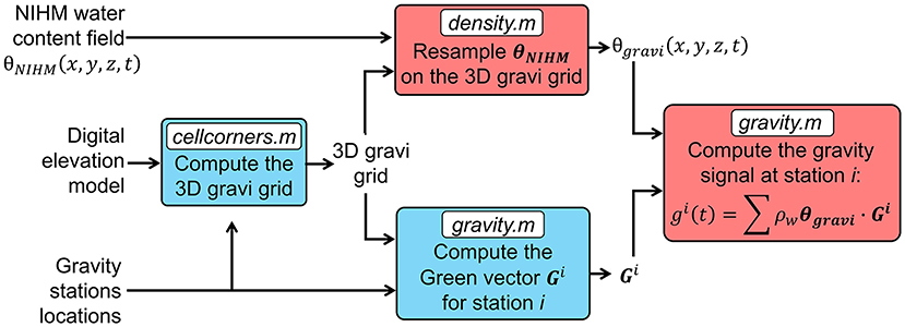
Figure 9. Principle of the Matlab® gravity forward modeling code developed to compute temporal gravity changes at the gravity stations from the 3D NIHM water content field. Blue boxes correspond to functions that are run only once while red boxes correspond to functions that are run at each timestep.
We only computed gravity changes for the 8 innermost stations (STR F5, STR PZ3, STR8, STR7, STR F8, STR F7, and STR4), because they are the less sensitive to the water dynamics occurring outside from the Strengbach catchment, which was not modeled by NIHM. These stations are defined so that the maximal external gravity signal i.e., coming from outside the catchment, is <25 nm.s−2, which corresponds to half the typical uncertainty found when performing relative gravity measurements with a Scintrex CG5 gravimeter (e.g., Christiansen et al., 2011; McClymont et al., 2012; Arnoux et al., 2020). We computed this maximal external signal as the gravity effect of a 0,250 m thick water layer draped on the topography outside from the Strengbach catchment. This water layer is an upper bound of catchment water balance range within the last 10 years as inferred from OHGE data.
Estimated Hydrogravimetric Variations vs. Measurements
Observed and modeled gravity time series are shown in Figure 4, and the state of the water content estimated by NIHM is shown Figure 10 for two dates. The first date (the 19 of March 2019) corresponds to a gravity survey made in wet conditions with high water volume stored in the catchment (Figure 10A), while the second one (the 12 of September 2019) corresponds to a gravity survey made in dry conditions with low water volume stored in the catchment (Figure 10B). Water storage simulated by NIHM exhibits low change between the wet and the dry period (Figure 10C), except in the colluvium accumulation area and in the valley bottom where the water stock decrease can reach, respectively −0.46 and −0.90 m of water. Hence, WSC beneath the gravity stations is only significant for STRF8 (−0.60 m), STRF5 (−0.30 m), and STR4 (−0.30 m), while it is smaller than −0.05 m for the other stations.
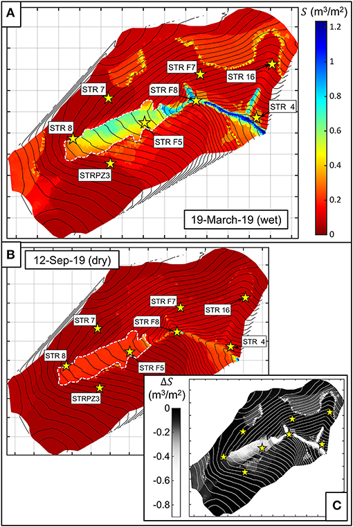
Figure 10. Spatial distribution of water storage as modeled by NIHM. (A) Water volume estimated by NIHM for a wet period (19th March 2019), just after a snowmelt event. (B) Water volume estimated by NIHM for a dry period (12th September 2019) at the end of Summer. (C) Difference of water storage between the wet and the dry period.
For the station STR F5, there is a good coincidence in time between observed and modeled maximal values occurring on the 19th March of 2019 and on the 2nd of February 2020 (Figure 4D). The gravity decrease observed during the March–September 2019 discharge period is relatively well-reproduced by the model, and one can also note the good correspondence between observed and modeled gravity changes during the January–February 2020 period. However, for both May–September 2018 and March–September 2019 periods, observed gravity changes have a significantly larger range (respectively, 192 ± 65 2 and 219 ± 45 nm.s−2) than modeled gravity changes estimated at the measurement dates (respectively, 29 and 110 nm.s−2). This range difference results from a lower decrease of modeled gravity compared to observed gravity during the dry periods of July-September 2018 and 2019, as modeled gravity reached a low plateau in July while observed gravity continued decreasing until September. The range difference also results from a lower maximal value for modeled gravity changes compared to the gravity value measured in March 2019 and June 2018. In June 2018, measured gravity reached 121 ± 60 nm.s−2 while modeled gravity value is 1 nm.s−2. In March 2019, observed gravity reached 129 ± 30 nm.s−2 while modeled gravity value is 84 nm.s−2.
For the station STR F8, although both observed and modeled gravity changes exhibit a similar range, they significantly differ from each other (Figure 4D), resulting in a high χ2 value of 9.5 (Table 2). Modeled gravity varies between a high plateau, when the medium beneath the station is water saturated, and a low plateau, when the underlying medium is desaturated. We do not observe these features in measured gravity, which is increasing during the May–September 2018 draining period while modeled gravity is increasing, and which is decreasing during the March–May 2019 period, while modeled gravity is stable.
For station STR4, modeled and observed gravity have a similar range (Figure 4D), but they also significantly differ from each other, as during the June–July 2019 period when modeled gravity decrease while observed gravity increase, resulting in a χ2 value of 6.4 (Table 2).
For the station STR7, observed gravity changes have a much larger range than modeled gravity changes as a result of the very low WSC beneath the gravity station (Figures 4, 10): the observed gravity range is 154 ± 45 nm.s−2 for the May–September 2018 period, and 144 ± 14 nm.s−2 for the March–September 2019 period, while the range of modeled gravity estimated at the measurement dates is, respectively, 8 and 12 nm.s−2. The same observation also applies for stations STR PZ3, STR F7, STR8, and STR16, which result in high χ2 values (Figure 4; Table 2).
Limits of the Approach
In this study, instead of directly converting Δg into WSC which require strong hypothesis about the spatial distribution of WSC (Arnoux et al., 2020; Halloran, 2021), we compared the gravity observations with gravity changes modeled from NIHM to infer water storage dynamics in the catchment. So that we use NIHM to interpret the gravity measurements in the one hand, and we use the gravity measurements to evaluate the model in the other hand. In accordance with the TWI approach, NIHM predicts the existence of an area with large WSC in the colluvium zone (Figure 10), which can explain the seasonal gravity changes of large amplitude observed at the STR F5 station, although the range of observed gravity changes is larger (Figure 4D; Table 2). For other stations, we could not reproduce observed gravity changes with the current version of the NIHM model (i.e., only calibrated on MRS and streamflow data), even qualitatively: For stations located in the valley bottom, observed and modeled gravity exhibit large discrepancies in term of temporal pattern (Figure 4D), while for stations located along the slopes, modeled gravity changes are of much lower amplitude than the observed one (Figure 4), as a result of the too low WSC modeled by NIHM (Figure 10C).
When computing temporal gravity changes, we made an explicit 3D calculation, so that discrepancies between modeled and observed gravity result either from: (i) the NIHM model structure or ii) the NIHM model calibration. By construction, NIHM can only model shallow water dynamics (section Water cycle monitoring), so that deeper water circulation pathways in the granitic bedrock fractures (as evidenced in deep boreholes, Ranchoux et al., 2021) is not taken into account with this modeling approach, which makes hypothesis (i) plausible. However, the analysis of the geochemical signatures of the spring water and the water collected from observation wells (>50 m deep boreholes and <15 m deep piezometer) showed that the springs water and the piezometers water circulate within the same surface aquifer with a low water residence time, while the water from the deep boreholes circulates in a distinct circulation system, within the fracture network of the granitic bedrock, and is characterized by much higher residence times (Chabaux et al., 2017; Ranchoux et al., 2021). So that when modeling water dynamics inside the Strengbach catchment, neglecting deep water circulation—as it is done by NIHM- is a reasonable hypothesis. Hence, hypothesis (ii) is our preferred hypothesis to explain the misfit between observed and modeled gravity. Indeed, when calibrating NIHM, only the thickness e and the saturated water content profile θS(z) were explored to fit the MRS data and the discharge at outlet, while other parameters were set to uniform values across the whole catchment (see section NIHM and Lesparre et al., 2020) although most of them, especially the hydraulic conductivity, are certainly spatially variables. Lesparre et al. (2020) also noted that MRS and discharge data are subjected to equifinality issues when seeking the porosity and the thickness of the watered layers, so that complementary information is required to better constrain these parameters. Hence, these equifinality issues and the lack of constrains on the hydraulic conductivity could explain the misfit between NIHM and observed gravity. Hybrid gravity data point toward a large increase in WSC amplitude compared to the current NIHM model, which could be obtained by increasing the porous volume (i.e., the product of the thickness with the porosity) below the gravity stations and decreasing the hydraulic conductivity downstream of the stations. Hybrid gravity data could hence contribute to build a more robust model of the subsurface hydrodynamic properties, which would improve the understanding of water dynamics inside a mountain catchment within a multi-method calibration exercise.
Perspectives
In this study we showed that the current version of NIHM (i.e., only calibrated on MRS and streamflow) cannot simulate the water dynamics properly, especially along the slopes were modeled WSC are of much too small amplitude. So that a multi method calibration exercise of the NIHM model is required. Such multi-method calibration would take advantage of the complementarity between gravimetry and MRS which brings constrains on the vertical distribution of the water content (Mazzilli et al., 2016), as well with seismic refraction (Flinchum et al., 2018) that bring information on the subsurface structure, in particular on the saprolite thickness. So that we first need to: (i) finely understand the impact of gravity station locations on the gravity signal footprint by using the hydro-gravimetric framework we presented in this study and (ii) analyze the sensitivity of the gravimetric signal to hydrodynamics parameters, in order to identify parameters that can be effectively constrained with gravimetry.
From a pure measurement point of view, the monthly gravity monitoring we performed allowed to identify STR F5 as a station with large–and thus easily measurable–temporal gravity changes. It would hence be very interesting to implement at STR F5 a high-frequency gravity timelapse measurement campaign (i.e., with a weekly interval during 2 months) to highlight possible rapid variations of the water stock, taking place on a daily or weekly scale. Such measurement campaign would idealy target the draining period that occur just after the last large snowmelt event of the winter season, like the one that occurred in mid-March 2019 (Figure 2C; Chaffaut et al., 2022). Such experiment will be implemented in a future work. It should allow to confirm the large storage capacity of the colluvium zone revealed by monthly hybrid gravity monitoring but also to finely constrain its hydraulic conductivity.
In this study, we focused on a particular granitic mountain catchment with an oceanic-mountainous climate. However, it would be particularly interesting to take advantage of the international network of critical zone observatories (e.g., Anderson et al., 2008; White et al., 2015; Brantley et al., 2017; Gaillardet et al., 2018) to implement hybrid gravity monitoring on mountain watersheds with different geology and/or climate. Indeed, most of these study sites are already well-characterized in term of topography and geomorphology, and basic hydro-climatic variables–such as those used in this study—already benefit from continuous monitoring and fulfill the FAIR requirement (e.g., for the OZCAR infrastructure: see Gaillardet et al., 2018; Braud et al., 2020). These sites would therefore benefit the best from time-lapse hybrid gravity monitoring. A similar hybrid gravity approach should hence be transposed to these sites with some modifications: the high-cost superconducting gravimeters which serve as gravity reference in this study could be replaced by an FG5 absolute gravimeter (e.g., Sugihara and Ishido, 2008; Jacob et al., 2010), which would be deployed for each timelapse at a reference station accessible by car. As far as possible, the reference station should be located on a summit, so that all of WSC are occurring below it and hence contribute in a cumulative way to the measured gravity signal, which would maximize its amplitude and ease the interpretation of gravity observations (Chaffaut et al., 2022). Micro-gravimetric stations should then be deployed on areas exempt from landslides or strong erosion-deposition processes, because those also induce temporal gravity changes that are indistinguishable from gravity changes due to hydrological processes, in the absence of comprehensive complementary information (Mouyen et al., 2012). Micro-gravimetric stations should be located on stable outcropping rocks or cemented pillars, and their positions should be regularly measured by differential GNSS or leveling techniques, to assess stations vertical motion (Ferhat et al., 2017). For performing the micro-gravimetric measurements, relative gravimeters (Scintrex CG5 or CG6) should be carried by hand between stations to minimize transport-induce perturbations (mechanical shocks, instrument tilting) which can induce significant hysteresis and measurement offsets (Flury et al., 2007; Reudink et al., 2014; Repanic and Kuhar, 2018). Micro-gravimetric stations should be measured several times in independent measurement loops during the same survey to assess the repeatability of the relative gravity measurements (Annex A). We also remind that in a mountainous context, time-lapse gravimetry requires accurately calibrated relative gravimeters (i.e., at the 10−5 level, see section Calibration of relative gravimeters), whose calibration factor stability need to be checked regularly (Cheraghi et al., 2019).
We note the recent arrival of new field gravimeters such as the Muquans® Quantum Absolute field Gravimeter (AQG) (Ménoret et al., 2018; Cooke et al., 2021), whose ability to accurately measure gravity changes (i.e., on the order of 10 nm.s−2) caused by rainfall events has been clearly demonstrated by Cooke et al. (2021) while the instrument was in continuous acquisition mode in an observatory. AQG presents the two-fold advantage of being easier to transport than the state-of-the-art FG5 absolute gravimeter (although it stills require a car) and much easier to operate in field condition (Güntner et al., 2021), as the setting up is faster (i.e., ~30 min) and the measurement time is shorter (i.e., ~1 h). Güntner et al. (2021) conducted a preliminary experiment demonstrating a repeatability of 40 ± 35 nm.s−2 for the field version of the AQG. So that this instrument could be used to perform potentially less labor-intensive time lapse gravity monitoring experiments, with a repeatability similar to that obtained in this study.
We also note the particularly rapid development of new types of MEMS (Micro Electro Mechanical Systems) gravimeters, which are more robust, less cumbersome and much cheaper than usual gravimeters. These MEMS gravimeters are currently “only” capable of measuring the tidal signal (e.g., Tang et al., 2019). However, the level of achieved accuracy will likely increase substantially in the coming years, so that they could potentially be used to monitor WSC on a continuous basis on a stations network.
Conclusion
We performed a hybrid gravity monitoring experiment to assess the spatio-temporal dynamics of water storage changes within the Strengbach mountain catchment. For this purpose, we measured gravity temporal changes over a network of 16 stations during two hydrological cycles combining a continuous gravity monitoring at a reference station made with a superconducting gravimeter with time lapse microgravimetry made with a Scintrex CG5 field relative gravimeter. Depending on the station, there are strong contrasts in terms of amplitude of gravity temporal changes but also in terms of temporal pattern as some stations exhibit a clear seasonal cycle while others exhibit lower or more complex temporal changes. These characteristics of the gravity signal reveal seasonal water storage changes heterogeneities within the catchment. Gravity observations have been discussed by means of the topographic wetness index and by means of a physically based distributed hydrological model. This study demonstrates the ability of hybrid gravimetry to assess the water storage dynamics in the Strengbach mountain catchment, which contributes to a better understanding of the hydrological processes occurring in mountain hydro-systems in general. Last but not least, our gravity dataset provides observations not presumed by the applied physically based distributed hydrological model, indicating that this model is currently under-constrained, which likely result from the relatively large number of parameters required to capture the spatial heterogeneity of the catchment subsurface. Hybrid gravimetry therefore appears as a very promising measurement method to condition such distributed hydrological model. This calibration exercise will be put into practice and presented in a coming paper.
Data Availability Statement
The raw data supporting the conclusions of this article are available at: https://hplus.ore.fr/en/chaffaut-et-al-2021-frontiers-in-water-data.
Author Contributions
QC: conceptualization, methodology, software, formal analysis, investigation, data curation, writing—original draft, and writing—review and editing. NL: conceptualization, methodology, software, data curation, and writing—review and editing. FM: conceptualization, methodology, writing—review & editing, and supervision. JH: conceptualization, methodology, writing—review and editing, supervision, and funding acquisition. DV: resources, data curation, and supervision. J-DB: resources and data curation. GF and SC: resources, data curation, and writing—review and editing. All authors contributed to the article and approved the submitted version.
Funding
The installation of the iGrav30 superconducting gravimeter has been funded by EQUIPEX CRITEX (https://www.critex.fr). The doctoral school ED413 from the Strasbourg university, as well as ANR HYDROCRIZSTO ANR-15-CE01-0010-02 and the OZCAR network (http://ozcar-ri.prod.lamp.cnrs.fr/) provided the funding for this study.
Conflict of Interest
The authors declare that the research was conducted in the absence of any commercial or financial relationships that could be construed as a potential conflict of interest.
Publisher's Note
All claims expressed in this article are solely those of the authors and do not necessarily represent those of their affiliated organizations, or those of the publisher, the editors and the reviewers. Any product that may be evaluated in this article, or claim that may be made by its manufacturer, is not guaranteed or endorsed by the publisher.
Acknowledgments
We are very grateful for the considerable work done by the editor and three reviewers which greatly improved the quality of this paper. We thank OHGE (http://ohge.unistra.fr/) for providing all hydro-meteorological data used in this study. We thank Julie Croisette and Célia Grün for having performed the microgravity surveys during Summer 2019. We also thank Sylvain Pasquet, Guillaume Modeste, Romain Pestourie, Matthias Oursin, Damian Kula, and Sophie Chaffaut for their generous support during the extensive fieldwork. Last but not least, we thank Marianne Oudin for her warm welcome at Les Grands Prés guest houses in Aubure.
Supplementary Material
The Supplementary Material for this article can be found online at: https://www.frontiersin.org/articles/10.3389/frwa.2021.715298/full#supplementary-material
References
Anderson, S. P., Bales, R. C., and Duffy, C. J. (2008). Critical zone observatories: building a network to advance interdisciplinary study of earth surface processes. Mineral. Magaz. 72, 7–10. doi: 10.1180/minmag.2008.072.1.7
Arnoux, M., Halloran, L. J. S., Berdat, E., and Hunkeler, D. (2020). Characterizing seasonal groundwater storage in alpine catchments using time-lapse gravimetry, water stable isotopes and water balance methods. Hydrol. Process. 34, 4319–4333. doi: 10.1002/hyp.13884
Bales, R. C., Molotch, N. P., Painter, T. H., Dettinger, M. D., Rice, R., and Dozier, J. (2006). Mountain hydrology of the western United States. Water Resour. Res. 42:W08432. doi: 10.1029/2005WR004387
Beaulieu, E., Lucas, Y., Viville, D., Chabaux, F., Ackerer, P., Godderis, Y., et al. (2016). Hydrological and vegetation response to climate change in a forested mountainous catchment. Model. Earth Syst. Environ. 2:191. doi: 10.1007/s40808-016-0244-1
Beniston, M., and Stoffel, M. (2014). Assessing the impacts of climatic change on mountain water resources. Sci. Total Environ. 493, 1129–1137. doi: 10.1016/j.scitotenv.2013.11.122
Beven, K. J., and Kirkby, M. J. (1979). A physically based, variable contributing area model of basin hydrology. Hydrol. Sci. J. 24, 43–69. doi: 10.1080/02626667909491834
Bogena, H. R., Huisman, J. A., Güntner, A., Hübner, C., Kusche, J., Jonard, F., et al. (2015). Emerging methods for noninvasive sensing of soil moisture dynamics from field to catchment scale: a review. WIREs Water 2, 635–647. doi: 10.1002/wat2.1097
Boucher, M., Pierret, M. C., Dumont, M., Viville, D., and Legchenko, A. (2015). “MRS characterisation of a mountain hard rock aquifer: the Strengbach Catchment, Vosges Massif, France,” in MRS 2015 6th International Workshop on Magnetic Resonance Sounding (Aarhus).
Brantley, S. L., McDowell, W. H., Dietrich, W. E., White, T. S., Kumar, P., Anderson, S. P., et al. (2017). Designing a network of critical zone observatories to explore the living skin of the terrestrial Earth. Earth Surf. Dyn. 5, 841–860. doi: 10.5194/esurf-5-841-2017
Braud, I., Chaffard, V., Coussot, C., Galle, S., Juen, P., Alexandre, H., et al. (2020). Building the information system of the French critical zone observatories network: theia/OZCAR-IS. Hydrol. Sci. J. 1–19. doi: 10.1080/02626667.2020.1764568
Chabaux, F., Viville, D., Lucas, Y., Ackerer, J., Ranchoux, C., Bosia, C., et al. (2017). Geochemical tracing and modeling of surface and deep water–rock interactions in elementary granitic watersheds (Strengbach and Ringelbach CZOs, France). Acta Geochim. 36, 363–366. doi: 10.1007/s11631-017-0163-5
Chaffaut, Q., Hinderer, J., Masson, F., Viville, D., Bernard, J. D., Cotel, S., et al. (2020). “Continuous monitoring with a superconducting gravimeter as a proxy for water storage changes in a mountain catchment,” in International Association of Geodesy Symposia (Berlin: Springer). doi: 10.1007/1345_2020_105
Chaffaut, Q., Hinderer, J., Masson, F., Viville, D., Pasquet, S., Boy, J. P., et al. (2022). New insights on water storage dynamics in a mountainous catchment from superconducting gravimetry. Geophys. J. Int. 228, 432–446. doi: 10.1093/gji/ggab328
Champollion, C., Deville, S., Chéry, J., Doerflinger, E., Le Moigne, N., Bayer, R., et al. (2018). Estimating epikarst water storage by time-lapse surface-to-depth gravity measurements. Hydrol. Earth Syst. Sci 22, 3825–3839. doi: 10.5194/hess-22-3825-2018
Cheraghi, H., Hinderer, J., Abdoreza Saadat, S., Bernard, J. D., Djamour, Y., Tavak, F., et al. (2019). Stability of the calibration of scintrex relative gravimeters as inferred from 12 years of measurements on a large amplitude calibration line in Iran. Pure Appl. Geophys. 177, 991–1004. doi: 10.1007/s00024-019-02300-6
Christiansen, L., Binnning, P. J., Rosbjerg, D., Andersen, O. B., and Bauer-Gottwein, P. (2011). Using time-lapse gravity for groundwater model calibration: an application to alluvial aquifer storage. Water Resour. Res. 47, W06503. doi: 10.1029/2010WR009859
Cooke, A.-K., Champollion, C., and Le Moigne, N. (2021). First evaluation of an absolute quantum gravimeter (AQG#B01) for future field experiments. Geosci. Instrum. Method Data Syst. 10, 65–79. doi: 10.5194/gi-10-65-2021
Creutzfeldt, B., Ferré, T., Troch, P., Merz, B., Wziontek, H., and Güntner, A. (2012). Total water storage dynamics in response to climate variability and extremes: Inference from long-term terrestrial gravity measurement. J. geophys. Res. Atmosph. 117, D08112. doi: 10.1029/2011JD016472
Creutzfeldt, B., Güntner, A., Klügel, T., and Wziontek, H. (2008). Simulating the influence of water storage changes on the superconducting gravimeter of the geodetic observatory wettzell, Germany. Geophysics 73, WA95. doi: 10.1190/1.2992508
Davis, K., Li, Y., and Batzle, M. (2008). Time-lapse gravity monitoring: a systematic 4D approach with application to aquifer storage and recovery. Geophysics 73, WA61. doi: 10.1190/1.2987376
Delobbe, L., Watlet, A., Wilfert, S., and Van Camp, M. (2019). Exploring the use of underground gravity monitoring to evaluate radar estimates of heavy rainfall. Hydrol. Earth Syst. Sci. 23, 93–105. doi: 10.5194/hess-23-93-2019
Deville, S., Jacob, T., Chéry, J., and Champollion, C. (2013). On the impact of topography and building mask on time varying gravity due to local hydrology. Geophys. J. Int. 192, 82–93. doi: 10.1093/gji/ggs007
El Gh'Mari (1995). Etude Minéralogique, Pétrophysique et Géochimique de la Dynamique D'altération D'un Granite Soumis Aux Dépots Atmosphériques Acides (Bassin Versant du Strengbach, Vosges, France): Mécanismes, Bilans et Modélisations. (Ph.D. dissertion), Strasbourg 1 University, Strasbourg (France).
Elkin, C., Gutiérrez, A. G., Leuzinger, S., Manusch, C., Temperli, C., Rasche, L., et al. (2013). A 2 °C warmer world is not safe for ecosystem services in the European Alps. Glob. Change Biol. 19, 1827–1840. doi: 10.1111/gcb.12156
Ferhat, G., Portier, N., Hinderer, J., Calvo Garcia-Maroto, M., Abdelfettah, Y., and Riccardi, U. (2017). “Three years of monitoring using leveling and hybrid gravimetry applied to geothermal sites of Soultz-sous-Forêts and Rittershoffen, Rhine Graben, France,” in: International Conference Engineering Surveying (Lisbon).
Fichter, J., Dambrine, E., Turpault, M. P., and Ranger, J. (1998). Base cation supply in spruce and beech ecosystems of the Strengbach catchment (Vosges mountains, NE France). Water Air Soil Pollut. 104, 125–148. doi: 10.1023/A:1004966302517
Flinchum, B. A., Steven Holbrook, W., Rempe, D., Moon, S., Riebe, C. S., Carr, B. J., et al. (2018). Critical zone structure under a granite ridge inferred from drilling and three-dimensional seismic refraction data. J. Geophys. Res. Earth Surf. 123, 1317–1343. doi: 10.1029/2017JF004280
Flury, J., Peters, T., Schmeer, M., Timmen, L., Wilmes, H., and Falk, R. (2007). “Precision gravimetry in the new Zugspitze gravity meter calibration system,” in Proceedings of the 1st International Symposium of the International Gravity Field Service (Istanbul).
Fores, B., Champollion, C., Le Moigne, N., and Chery, J. (2016). Impact of ambient temperature on spring-based relative gravimeter measurements. J. Geod. 91, 269–277. doi: 10.1007/s00190-016-0961-2
Gaillardet, J., Braud, I., Hankard, F., Anquetin, S., Bour, O., Dorfliger, N., et al. (2018). OZCAR: the French network of critical zone observatories. Vadose Zone J. 17:180067. doi: 10.2136/vzj2018.04.0067
Gehman, C. L., Harry, D. L., Sanford, W. E., Stednick, J. D., and Beckman, N. A. (2009). Estimating specific yieldand storage change in an unconfined aquifer using temporal gravity surveys. Water Resour. Res. 45:W00D21. doi: 10.1029/2007WR006096
Grabs, T., Seibert, J., Bishop, K., and Laudon, H. (2009). Modeling spatial patterns of saturated areas: a comparison of the topographic wetness index and a dynamic distributed model. J. Hydrol. 373, 15–23. doi: 10.1016/j.jhydrol.2009.03.031
Granier, A., Bréda, N., Biron, P., and Villette, S. (1999). A lumped water balance model to evaluate duration and intensity of drought constraints in forest stands. Ecol. Model 116, 269–83. doi: 10.1016/S0304-3800(98)00205-1
Güntner, A., Reich, M., Reinhold, A., Glässel, J., and Wziontek, H. (2021). First Experiences With an Absolute Quantum Gravimeter During Field Campaigns. EGU General Assembly 2021. doi: 10.5194/egusphere-egu21-14072
Halloran, L. J. S. (2021). Improving groundwater storage change estimates using time-lapse gravimetry with Gravi4GW. Earth Space Sci. Open Arch. doi: 10.1002/essoar.10507438.1
Hector, B., Seguis, L., Hinderer, J., Cohard, J.-M., Wubda, M., Descloitres, M., et al. (2015). Water storage changes as a marker for base flow generation processes in a tropical humid basement catchment (Benin): insights from hybrid gravimetry. Water Resour. Res. 51, 8331–8361. doi: 10.1002/2014WR015773
Henrion, E., Masson, F., Doubre, C., Ulrich, P., and Meghraoui, M. (2020). Present-day deformation in the Upper Rhine Graben from GNSS data. Geophys. J. Int. 223, 599–611. doi: 10.1093/gji/ggaa320
Hinderer, J., Crossley, D., and Warburton, R. J. (2015). “Superconducting Gravimetry,” in Treatise on Geophysics, 2nd edn, Vol. 3, ed G. Schubert (Oxford: Elsevier), 59–115. doi: 10.1016/B978-0-444-53802-4.00062-2
Hinderer, J., Hector, B., Mémin, A., and Calvo, M. (2016). Hybrid gravimetry as a tool to monitor surface and underground mass changes. Int. Assoc. Geodesy Symp. 147, 123–130. doi: 10.1007/1345_2016_253
Jacob, T., Bayer, R., Chery, J., Jourde, H., Le Moigne, N., Boy, et al. (2008). Absolute gravity monitoring of water storage variation in a karst aquifer on the larzac plateau (Southern France). J. Hydrol. 359, 105–117. doi: 10.1016/j.jhydrol.2008.06.020
Jacob, T., Bayer, R., Chery, J., and Le Moigne, N. (2010). Time-lapse microgravity surveys reveal water storage heterogeneity of a karst aquifer. J. Geophys. Res. 115:B06402. doi: 10.1029/2009JB006616
Jeannot, B., Weill, S., Eschbach, D., Schmitt, L., and Delay, F. (2018). A low-dimensional integrated subsurface hydrological model coupled with 2-D overland flow: application to a restored fluvial hydrosystem (Upper Rhine River – France). J. Hydrol. 563, 495–509. doi: 10.1016/j.jhydrol.2018.06.028
Kennedy, J., Ferré, T. P. A., and Creutzfeldt, B. (2016). Time-lapse gravity data for monitoring and modeling artificial recharge through a thick unsaturated zone. Water Resour. Res. 52, 7244–7261. doi: 10.1002/2016WR018770
Kennedy, J. R., and Ferré, T. P. A. (2016). Accounting for time- and space-varying changes in the gravity field to improve the network adjustment of relative-gravity data. Geophys. J. Int. 204, 892–906. doi: 10.1093/gji/ggv493
Ladouche, B., Probst, A., Viville, D., Idir, S., Baque, D., Loubet, M., et al. (2001). Hydrograph separation using isotopic, chemical and hydrological approaches (Strengbach catchment, France). J. Hydrol. 242, 255–274. doi: 10.1016/S0022-1694(00)00391-7
Leirião, S., He, X., Christiansen, L., Andersen, O. B., and Bauer-Gottwein, P. (2009). Calculation of the temporal gravity variation from spatially variable water storage change in soils and aquifers. J. Hydrol. 365, 302–309. doi: 10.1016/j.jhydrol.2008.11.040
Lesparre, N., Girard, J. F., Jeannot, B., Weill, S., Dumont, M., Boucher, M., et al. (2020). Magnetic resonance sounding measurements as posterior information to condition hydrological model parameters: application to a hard-rock headwater catchment. J. Hydrol. 587:124941. doi: 10.1016/j.jhydrol.2020.124941
Longuevergne, L., Boy, J. P., Florsch, N., Viville, D., Ferhat, G., Ulrich, P., et al. (2009). Local and global hydrological contributions to gravity variations observed in Strasbourg. J. Geodyn. 48, 189–194. doi: 10.1016/j.jog.2009.09.008
Masson, F., Viville, D., Pierret, M.-C., Mouyen, M., Hecker, L., and Chabaux, F. (2012). Time-lapse microgravity study of the Strengbach catchment (Vosges mountains, France). Cr. Geosci. 344, 357–365. doi: 10.1016/j.crte.2012.06.001
Mazzilli, N., Boucher, M., Chalikakis, K., Legchenko, A., Jourde, H., and Champollion, C. (2016). Contribution of magnetic resonance soundings for characterizing water storage in the unsaturated zone of karst aquifers. Geophysics 81, 49–61. doi: 10.1190/geo2015-0411.1
McClymont, A. F., Hayashi, M., Bentley, L. R., and Liard, J. (2012). Locating and characterising groundwater storage areas within an alpine watershed using time-lapse gravity, GPR and seismic refraction methods. Hydrol. Process 26, 1792–1804. doi: 10.1002/hyp.9316
Ménoret, V., Vermeulen, P., Le Moigne, N., Bonvalot, S., Bouyer, P., Landragin, A., et al. (2018). Gravity measurements below 10–9 g with a transportable absolute quantum gravimeter. Sci. Rep. 8:12300. doi: 10.1038/s41598-018-30608-1
Mouyen, M., Masson, F., Hwang, C., Cheng, C. C., Le Moigne, N., Lee, C. W., et al. (2012). Erosion effects assessed by repeated gravity measurements in southern Taiwan. Geophys. J. Int. 192, 113–136. doi: 10.1093/gji/ggs019
Naujoks, M., Kroner, C., Weise, A., Jahr, T., Krause, P., and Eisner, S. (2010). Evaluating local hydrological modelling by temporal gravity observations and a gravimetric three-dimensional model: gravity and hydrology: local 3-D modelling. Geophys. J. Int. 182, 233–249. doi: 10.1111/j.1365-246X.2010.04615.x
Naujoks, M., Weise, A., Kroner, C., and Jahr, T. (2008). Detection of small hydrological variations in gravity by repeated observations with relative gravimeters. J. Geod. 82, 543–553. doi: 10.1007/s00190-007-0202-9
Niebauer, T. M., Sasagawa, S., Fallel, J. E., Hilt, R., and Klopping, E. (1995). A new generation of absolute gravimeters. Metrologia 32, 159–180. doi: 10.1088/0026-1394/32/3/004
Okubo, S., Satomura, M., Furuya, M., Sun, W., Matsumoto, S., Ueki, S., et al. (2002). “Grand design for the hybrid gravity network around the Mt. Fuji volcano,” in International Symposium on Geodesy in Kanazawa, 39–40.
Pearson-Grant, S. C., Franz, P., and Clearwater, J. (2018). Gravity measurements as a calibration tool for geothermal reservoir modelling. Geothermics 73, 146–157. doi: 10.1016/j.geothermics.2017.06.006
Pfeffer, J. (2011). Etude du Cycle de l'eau en Afrique Sahélienne : Approche Multidisciplinaire et Apport de la Gravimétrie Terrestre et Spatiale. (Thèse de doctorat), University de Strasbourg, Strasbourg (France).
Pfeffer, J., Champollion, C., Favreau, G., Cappelaere, B., Hinderer, J., Boucher, M., et al. (2013). Evaluating surface and subsurface water storage variations at small time and space scales from relative gravity measurements in semiarid Niger. Water Resour. Res. 49, 3276–3291. doi: 10.1002/wrcr.20235
Pierret, M. C., Cotel, S., Ackerer, P., Beaulieu, E., Benarioumlil, S., Boucher, M., et al. (2018). The Strengbach catchment: a multidisciplinary environmental sentry for 30 years. Vadose Zone J. 17:180090. doi: 10.2136/vzj2018.04.0090
Pool, D. R. (2008). The utility of gravity and water-level monitoring at alluvial aquifer wells in southern Arizona. Geophysics 73, 49–59. doi: 10.1190/1.2980395
Pool, D. R., and Schmidt, W. (1997). Measurement of Ground-Water Storage Change and Specific Yield Using the Temporal-Gravity Method Near Rillito Creek. Water-Resources Investigations Report. Tucson Arizona, US Department of the Interior, US Geological Survey. 97, 4125.
Portier, N., Hinderer, J., Riccardi, U., Ferhat, G., Calvo, M., Abdelfettah, Y., et al. (2018). Hybrid gravimetry monitoring of Soultz-sous-Forêts and Rittershoffen geothermal sites (Alsace, France). Geothermics 76, 201–219. doi: 10.1016/j.geothermics.2018.07.008
Ranchoux, C., Chabaux, F., Viville, D., Thierry, L., Yann, L., Van der Woerd, J., et al. (2021). Characterization of groundwater circulations in a headwater catchment from an analysis of chemical concentrations, Sr-Nd-U isotope ratios, and CFC, SF6 gas tracers (Strengbach CZO, France). Appl. Geochem. 131:105030. doi: 10.1016/j.apgeochem.2021.105030
Reich, M., Mikolaj, M., Blume, T., and Güntner, A. (2019). Reducing gravity gravity data for the influence of water storage variations beneath observatory buildings. Geophysics 84, 15–31. doi: 10.1190/geo2018-0301.1
Repanic, M., and Kuhar, M. (2018). Modelling hysteresis effect in Scintrex CG?3M gravity readings Geophysical Prospecting. 66, 257–269. doi: 10.1111/1365-2478.12557
Reudink, R., Klees, R., Francis, O., Kusche, J., Schlesinger, R., Shabanloui, A., et al. (2014). High tilt susceptibility of the Scintrex CG-5 relative gravimeters, J. Geod. 88, 617–622. doi: 10.1007/s00190-014-0705-0
Scintrex Limited (2012). CG5 Scintrex Autograv System Operation Manual. Concord, OT, Scintrex Limited.
Sørensen, R., Zinko, U., and Seibert, J. (2006). On the calculation of the topographic wetness index: evaluation of different methods based on field observations. Hydrol. Earth Syst. Sci. 10, 101–112. doi: 10.5194/hess-10-101-2006
Sugihara, M., and Ishido, T. (2008). Geothermal reservoir monitoring with a combination of absolute and relative gravimetry. Geophysics 73, WA37–WA47. doi: 10.1190/1.2991105
Tang, S., Liu, H., Yan, S., Xu, X., Wu, W., Fan, J., et al. (2019). A high-sensitivity MEMS gravimeter with a large dynamic range. Microsyst. Nanoeng. 5:45. doi: 10.1038/s41378-019-0089-7
Vereecken, H., Huisman, J. A., Pachepsky, Y., Montzka, C., van der Kruk, J., Bogena, H., et al. (2014). On the spatio-temporal dynamics of soil moisture at the field scale. J. Hydrol. 516, 76–96. doi: 10.1016/j.jhydrol.2013.11.061
Viviroli, D., Archer, D. R., Buytaert, W., Fowler, H. J., Greenwood, G. B., Hamlet, A. F., et al. (2011). Climate change and mountain water resources: overview and recommendations for research, management and policy. Hydrol. Earth Syst. Sci. 15, 471–504. doi: 10.5194/hess-15-471-2011
Viviroli, D., Dürr, H. H., Messerli, B., Meybeck, M., and Weingartner, R. (2007). Mountains of the world, water towers for humanity: typology, mapping, and global significance. Water Resour. Res. 43:W07447. doi: 10.1029/2006WR005653
Voigt, C., Schulz, K., Koch, F., Wetzel, K. F., Timmen, L., Rehm, T., et al. (2021). Introduction of a superconducting gravimeter as novel hydrological sensor for the alpine research catchment zugspitze. Hydrol. Earth Syst. Sci. 25, 5047–5064. doi: 10.5194/hess-25-5047-2021
Warburton, R. J., Pillai, H., and Reineman, R. C. (2010). “Initial results with the new GWR iGrav™ superconducting gravity meter,” in International Association of Geodesy (IAG) Symposium Proceedings. IAG Symposium on Terrestrial Gravimetry: Static and Mobile Measurements (TG-SMM2010) (Saint Petersburg).
Weill, S., Delay, F., Pan, Y., and Ackerer, P. (2017). A low-dimensional subsurface model for saturated and unsaturated flow processes: ability to address heterogeneity. Comput. Geosci. 21:301314. doi: 10.1007/s10596-017-9613-8
Keywords: time variable gravity, hybrid gravimetry, mountain headwater catchment, water storage dynamics, distributed hydrologic model
Citation: Chaffaut Q, Lesparre N, Masson F, Hinderer J, Viville D, Bernard J-D, Ferhat G and Cotel S (2022) Hybrid Gravimetry to Map Water Storage Dynamics in a Mountain Catchment. Front. Water 3:715298. doi: 10.3389/frwa.2021.715298
Received: 26 May 2021; Accepted: 26 November 2021;
Published: 03 January 2022.
Edited by:
Jean Marçais, INRAE Clermont-Auvergne-Rhône-Alpes, FranceReviewed by:
Luca Guillaumot, International Institute for Applied Systems Analysis (IIASA), AustriaTy Ferre, University of Arizona, United States
Landon J. S. Halloran, Université de Neuchâtel, Switzerland
Copyright © 2022 Chaffaut, Lesparre, Masson, Hinderer, Viville, Bernard, Ferhat and Cotel. This is an open-access article distributed under the terms of the Creative Commons Attribution License (CC BY). The use, distribution or reproduction in other forums is permitted, provided the original author(s) and the copyright owner(s) are credited and that the original publication in this journal is cited, in accordance with accepted academic practice. No use, distribution or reproduction is permitted which does not comply with these terms.
*Correspondence: Quentin Chaffaut, Y2hhZmZhdXQucXVlbnRpbkBnbWFpbC5jb20=