 Grégory Etangsale
 Vincent Fontaine
 Nalitiana Rajaonison‡
- PIMENT (EA 4518), Department of Building and Environmental Sciences, University of La Réunion, Le Tampon, France
The present paper discusses families of Interior Penalty Discontinuous Galerkin (IP) methods for solving heterogeneous and anisotropic diffusion problems. Specifically, we focus on distinctive schemes, namely the Hybridized-, Embedded-, and Weighted-IP schemes, leading to final matrixes of different sizes and sparsities. Both the Hybridized- and Embedded-IP schemes are eligible for static condensation, and their degrees of freedom are distributed on the mesh skeleton. In contrast, the unknowns are located inside the mesh elements for the Weighted-IP variant. For a given mesh, it is well-known that the number of degrees of freedom related to the standard Discontinuous Galerkin methods increases more rapidly than those of the skeletal approaches (Hybridized- and Embedded-IP). We then quantify the impact of the static condensation procedure on the computational performances of the different IP classes in terms of robustness, accuracy, and CPU time. To this aim, numerical experiments are investigated by considering strong heterogeneities and anisotropies. We analyze the fixed error tolerance versus the run time and mesh size to guide our performance criterion. We also outlined some relationships between these Interior Penalty schemes. Eventually, we confirm the superiority of the Hybridized- and Embedded-IP schemes, regardless of the mesh, the polynomial degree, and the physical properties (homogeneous, heterogeneous, and/or anisotropic).
1. Introduction
The Discontinuous Galerkin (DG) methods were firstly introduced by Reed and Hill (1973) for the neutron transport phenomenon. Since their introduction, the DG methods have become a relevant class of finite element schemes for modeling physical processes. They provide several advantages: they are locally conservative and eligible to hp-refinement strategies and they consider a discontinuous piecewise (polynomial) approximation of the exact solution (Arnold et al., 2002; Rivière, 2008; Pietro and Ern, 2011). During the 1980s, Arnold proposed the famous Interior Penalty Discontinuous Galerkin (IP) method for solving the second-order elliptic problem (Arnold, 1982). Even if the stability and robustness of the IP method have been proven for homogeneous media (Wheeler, 1978; Rivière, 2008), these benefits are no longer ensure in the presence of high heterogeneous, and/or anisotropic ratios (Burman and Zunino, 2006; Ern et al., 2009). To restore the robustness, these authors replace the standard average operator, in the IP formalism, with a weighted one accounting for the diffusivity in the normal direction. The resulting discretization scheme is well-known as the Weighted-Interior Penalty (WIP) method. However, despite all these beneficial features, the DG methods have been recognized to be generally more expensive than the standard Conforming Finite Element methods such as the Continuous Galerkin (CG) and the Mixed Finite Element (Peraire and Persson, 2008). The final matrix system of DG methods leads to a larger stencil with a higher number of coupled degrees of freedom (DOFs), which is quite challenging for large-scale problems (Rivière, 2008). Following these observations, Cockburn et al. (2009b) introduced a new DG discretization scheme to overcome these drawbacks called the Hybridized Discontinuous Galerkin (HDG) methods.
The HDG methods can be considered as a DG methods that are eligible for static condensation. An additional trace variable is introduced to approximate the exact solution on the mesh skeleton. This original unknown also belongs to the set of piecewise discontinuous functions (Nguyen et al., 2009; Wells, 2011; Cockburn et al., 2012; Fabien et al., 2020). Thus, the global coupled linear system can be reduced by static condensation only to the interface-based DOFs located on the mesh skeleton (Cockburn et al., 2009a; Nguyen et al., 2009; Lehrenfeld and Schöberl, 2016). Besides, the HDG methods provide a smaller and sparser matrix system, and they inherit the benefits of the traditionally DG methods. They have proven to be more robust and efficient than the standard DG schemes for many situations. Moreover, superconvergence of discrete variables can be attained by employing an appropriate local postprocessing technique (Nguyen et al., 2009; Cockburn et al., 2012; Dijoux et al., 2019). Recently, an alternative version of the HDG method has been developed to reduce the size of the final matrix system (Cockburn et al., 2009c). The corresponding discretization scheme is called the Embedded Discontinuous Galerkin method (EDG) and extends the concept of the trace variable to the set of continuous functions. This alternative approach providing less CPU time and a tighter stiffness matrix compared to the original HDG framework (Zhang et al., 2019). However, by enforcing the continuity of the discrete trace, the EDG method may have to afford a loss of accuracy for approximating the discrete solution (Cockburn et al., 2009c; Zhang et al., 2019; Fabien et al., 2020).
This manuscript compares the Hybridized-, Embedded-, and Weighted-Interior Penalty formalisms in terms of accuracy, efficiency, and computational cost. Previous works offered comparisons between the standard CG or DG versus the HDG methods (see, e.g., Woopen et al., 2014; Fidkowski, 2016, 2019) favoring the latest formalism at different scales. However, these studies are limited to basic situations that do not include the high variations of the physical properties of the medium (i.e., heterogeneity and/or anisotropy). The present work focuses specifically on the primal class of Interior Penalty method for heterogeneous and/or anisotropic diffusion problems. We provide an appropriate stabilization function inspired by Etangsale et al. (2021), which employs the normal diffusivity coefficient to improve the robustness of the IP method. Then, by quantifying the computational cost of the HIP, EIP, and WIP schemes, we prove the effects of the static condensation on the global matrix sparsity and CPU time for the Hybridized- and Embedded-IP methods. Clearly and without ambiguity, we demonstrate the superiority of both skeletal methods (Hybridized- and Embedded-IP) over the traditional DG techniques (standard IP and WIP). Besides, we established some relationships between the standard IP, WIP, and HIP schemes, whose results are similar to those discussed by Fabien et al. (2020) for a homogeneous permeability tensor. We also emphasize the total equivalence properties between the Incomplete HIP and WIP schemes assuming a specific definitions of (i) the weighting function and (ii) the penalization function. At least, we provided numerical experiments to corroborate the observations mentioned above, and to prove the robustness of each schemes considering heterogeneous and/or anisotropic characteristics.
The material is organized as follows. In section 2, we describe the model problem and precise our notations and the discrete settings. In section 3, we briefly describe the Hybridized-, Embedded-, and Weighted-Interior Penalty formalisms. We then quantify the number of globally coupled degrees of freedom of each schemes for a given mesh and a fixed polynomial degree. In section 5, numerical experiments are investigated using h- and p-refinement strategies, and we compare the computational performances of the IP methods for a wide range of heterogeneity and anisotropy. We conduct discussions to identify the most suitable IP formalism in terms of robustness, accuracy and computing time. Finally, we end with some concluding remarks and perspectives.
2. Problem Statement and Notations
2.1. Model Problem
Let Ω be a two-dimensional convex polygonal domain, and we denote by Γ: = ∂Ω its boundary such that, Γ: = ΓD ∪ ΓN and ΓD ∩ ΓN = ∅. Here, ΓD and ΓN represent the boundary parts of the domain where Dirichlet and Neumann boundary conditions are provided, respectively. The governing equation is described by the second-order elliptic problem
with the following boundary conditions,
where f represents a source or sink term, gD and gN the prescribed Dirichlet and Neumann boundary data, respectively. In the context of heterogeneous and anisotropic processes, the permeability tensor κ is assumed to be a symmetric positive-definite matrix-valued function.
2.2. Mesh Assumptions
Let us introduce some discrete notations associated to the partition of the domain. We consider the family , which consists of a collection of polygonal elements. We specify here that the set refers to an affine triangulation of the domain Ω. For all , we denote by |A| its measure and by hA its diameter such that . Let ∂A be the boundary of an element of the mesh . In the rest of the document, we will prefer the generic term interface in place of an edge of the triangulation. Let us denote by and the set of interior and boundary interfaces, respectively. We further assume that coincides with the Dirichlet and Neumann boundary parts such that, and . The subsets and refers to the set of all interfaces lying entirely into the Dirichlet and Neumann boundary parts, respectively. The set of all interfaces is provided by the mesh skeleton as . In the same way, we introduce the collection of all boundary interfaces for each elements of the triangulation such that, . For any given elements , and for any edges F ∈ ∂A, we denote nF, A as the unit normal vector to F pointing out of A.
2.3. Functional Spaces
We consider the polygonal domain D ⊂ ℝ2, with boundary ∂D. We denote by (·, ·)D and 〈·, ·〉∂D the standard L2-inner product in L2(D) and L2(∂D), respectively. Thus, we introduce the compact notations related to the discrete L2-inner scalar product :
with , and corresponds to their respective norms. As usual in families of Discontinuous Galerkin methods, we consider the following broken space inside the elements for the discretization:
where the discrete variable vh∈Vh is defined within each elements of the triangulation . For the Hybridized discretization of the Discontinuous Galerkin methods, the approximation requires an auxiliary variable which is called the trace variable. The numerical trace is defined on the skeleton with respect to the imposed Dirichlet boundary conditions, such that:
where πh denotes the L2-orthogonal projection onto . We refer to for the set of polynomial functions defined on the skeleton, and vanishing on the Dirichlet boundary ΓD. Here, denotes the space of polynomials at least degree k ≥ 1 on X, where X corresponds to a generic element of or .
2.4. Trace Operators
We denote by the composite variable associated to the pair of discrete spaces . For all and F ∈ ∂A, we define the HDG-jump operator of the composite variable across as . Since no confusions can arise, we omit the subscripts A and F from the definition, and we simply write . For any scalar- and vector- valued function, we introduce the standard DG-jump and weighted-average operators for each faces as follows,
where ω: = (ω1, ω2) is a weighting function verifying that the weights satisfy ω1+ω2 = 1. Similarly, we introduce the conjugate weighting function associated with ω. In particular, for the case ω = (1/2, 1/2), we recover the classical average operator, and we will omit the subscript ω in its definition.
3. Discretization of the Interior Penalty Methods
This section describes three primal DG schemes, namely, the Hybridized-, Embedded-, and Weighted-Interior Penalty methods. We provide a compact formulation of the corresponding discrete bilinear forms and evaluates the computational cost of the schemes. For readers unfamiliar with the Discontinuous Galerkin approach, we recommend the studies proposed by Arnold et al. (2002) and Cockburn et al. (2009b), which outline the concepts and ideas behind the standard and Hybridized DG methods in a unified framework.
3.1. Hybridized and Embedded IP Formulations
The HDG formalism as proposed in Cockburn et al. (2009b) and Cockburn et al. (2009a) supposes that the discrete trace is evaluated distinctly with a piecewise polynomial functions on the boundaries of the elements. This specific definition of the discrete trace will produce a significant number of degrees of freedom, due to the discontinuous nature of its approximation on the mesh skeleton. To reduce the trace-based degrees of freedom, an alternative possibility consists of the restriction of the trace space to the set of continuous functions on the skeleton (Cockburn et al., 2009c). By considering the approximation ûh ∈ Ṽh, g with the continuous space , then the discretization corresponds to the Embedded Discontinuous Galerkin method (Cockburn et al., 2009c; Fabien et al., 2020). For approximating the problem (1), we introduce the two discrete composite spaces and associated to the composite discrete variable uh. For clarity, Figure 1 gives an illustration of the distribution of degrees of freedom for the Hybridized- and Embedded-IP method with polynomial degree k = 1. Notice that the only difference between the Hybridized and Embedded scheme lies in the selection of the discrete trace space. Thus, the discretization consists to seek such that
where the upperscript X corresponds to the Hybridized—(H) or Embedded—(E) IP method, according to the discrete composite space selected (i.e., discontinuous or continuous). The bilinear form can be linearly decomposed as:
Here, we reported the parameter ϵ, which is associated to the variations of the XIP discretization, as mentioned in Rivière (2008) and Fabien et al. (2020). For ϵ = 1, we retrieve the Symmetric scheme (S-XIP), and the cases ϵ = {−1, 0} corresponds to both non-symmetric schemes, where ϵ = −1 (resp. ϵ = 0) denotes the Non-Symmetric (N-XIP) [respectively, incomplete (I-XIP)] variants. In particular, the last contribution of the bilinear form refers to the penalization term with the penalization function τF, A. Naturally, the selection of the parameter τF, A is quite delicate, since it affects strongly the stability and the accuracy of the method (see Etangsale et al., 2021 for the investigation of the well-posedness and error estimates of the HIP method). In the following, we give a specific definition of the stabilization function that is influenced by the diffusivity parameter κ such that:
where is the normal diffusivity coefficient for any element , and α a positive user-dependent constant. It is important to note that the penalization function is piecewise constant on and double-valued for any interfaces (τF,A1 ≠ τ F,A2).

Figure 1. Stencil for a generic element (triangle or edge in blue) for the Embedded—(A), Hybridized—(B), and Weighted—(C). Interior Penalty discretization with polynomial order k = 1. For all methods, the nodes corresponding to degrees of freedom for the generic element are marked as solid red dots.
Remark 1 (Links with Continuous Galerkin). Assuming corresponds to the approximation of the discrete trace of the EIP method, and is the solution provided by the Continuous Galerkin method. Then, only for k = 1 and ϵ = 1, the equivalence on is verified for all data g and f, independently from the penalization function τF, A and the physical properties of the media κ (see Appendix in Cockburn et al., 2009c for more details). The equivalence is not valid anymore for both non-symmetric variants N-EIP and I-EIP, as listed in Table 1.
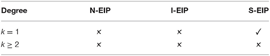
Table 1. Summary of the equivalence between the EIP and CG methods for various polynomial degrees k and different values of ϵ = {0, ±1}.
Since both the Hybridized- and the Embedded-IP methods are described identically through the definition (6), these schemes comprise the same benefit by applying the well-known static condensation technique (Cockburn et al., 2009b, 2012). This procedure was introduced for reducing the size of the global problem (6) to the only trace unknowns. Let us denote by Uh and the vector of DOFs associated to the element- and trace-based unknowns, respectively. Thus, the following global matrix system is obtained from the linear system (6):
where the vectors Fu and Gû are directly related to the source term and boundary conditions, respectively. Owing to the discontinuous nature of the space Vh, the matrix have a block-diagonal structure that allows its inversion. We are now able to substitute the global coupled matrix system (8) in terms of trace unknowns , in a such way that:
We notice that the left-hand side of the reduced linear system (9) is called the Shur complement of . Finally, the last step consists in the reconstruction of the discrete variable Uh element-by-element with the use of the relation:
The reduced version (9) leads to a smaller and symmetric matrix system easing the resolution.
3.2. Weighted IP Formulation
The Weighted-Interior Penalty (WIP) method were firstly introduced by Burman and Zunino (2006) in the context of advection-diffusion-reaction problems. The principal difference with the classical S-IP discretization proposed by Arnold Arnold (1982) resides in the use of a weighted average operators. In the WIP formulation proposed in Burman and Zunino (2006), Pietro and Ern (2011), and Dryja (2003), the weighting function only accounts for the variations of the diffusivity tensor κ from both sides of the mesh interfaces. In the following, we will favor a modified version of the weighting function depending on the penalization function of the Hybridized- or Embedded-IP methods as stated in Equation (7). Thus, the discretization of the WIP method consists to seek uh ∈ Vh such that
where the WIP bilinear form is given by:
and the linear form
contains the weakly imposed Dirichlet and Neumann boundary data. In Figure 1C, we depict the stencil of the WIP method, which is similar to the standard IP method. As in section 3.1, the parameter ϵ is used to control the introduction of the consistent symmetry term. Following its values, these methods are referred to as the Symmetric (ϵ = 1), the Non-Symmetric (ϵ = −1), and the Incomplete (ϵ = 0) schemes and are denoted S-WIP, N-WIP, and I-WIP, respectively. Let us now introduce the corresponding weighting function taking into account the values of the penalization from both sides of the interface as:
where the stabilization function τi = τF,Ai, for i = 1, 2, is defined by Equation (7). For all and F∈∂A, we give the penalization function as:
Remark 2 (Equivalence between the Hybridized- and Weighted-IP schemes). The numerical experiments performed in section 4 provided evidences for the total equivalence between the I-WIP and the I-HIP schemes, and for any values of τF, A satisfying the weighting (11) and the penalization function (12). Consequently, the Incomplete variations of the WIP and HIP methods conduct to the same robustness, accuracy, and stability. We would mention that these observations will be reported in a forthcoming work, where the total equivalence property will be mathematically demonstrated. Similar results can be found in Fabien et al. (2020) for the homogeneous case, where the I-HIP scheme coincides with the I-IP scheme (see Remark 3 for the characteristics of the corresponding IP scheme). However, this equivalence is not valid anymore for both Symmetric and Non-Symmetric IP variants.
Remark 3 (Relations with the standard IP method). Assuming now τ1 = τ2 for any interior interfaces , we then observe that ω = (1/2, 1/2) and the penalty function is simplified as . In this case, the WIP method is reduced to the standard IP method, where the well-known S-IP scheme was analyzed by Arnold (1982) and the N-IP scheme in Rivière (2008). From the definition (7) of the stabilization function, the WIP formulation is simplified to the standard IP method, if and only if the media is homogeneous and the partition is uniform (composed of geometrically identical elements).
3.3. Computational Cost
The purpose of this section is to illustrate the computational cost of the Hybridized- and Embedded-IP compared to the Weighted-IP method. By applying the static condensation procedure, the total number of degrees of freedom (DOFs) is reduced to the trace unknowns for both the HIP and EIP discretization. It appears that this quantity is proportional to the number of interfaces of the skeleton. For the WIP method, the global number of degrees of freedom is proportional to the number of elements of the partition . In order to ease the description, we consider a regular Cartesian domain Ω = [0, 1]2 partitioned into N × N squares. We distinguish two cases:
• The triangulation consists of a uniform rectangular grid made of N2 elements.
• The triangulation consists of a uniform triangular grid made of 2N2 elements, which is generated by divided each square into two triangles.
Now, we are able to compute the number of DOFs related to the methods under consideration. Let RH and RE be the ratio of DOFs of the HIP and EIP method versus the WIP method, such that:
where Nv, Ne, and NA refers to the number of vertices, edges, and elements (triangular/quadrilateral), respectively. The number of DOFs associated to the local reference element (interface or polygonal) can be defined by
In Figure 2, we display the computed ratios RH and RE for various polynomial degrees k and element sizes. Figures 2A,C show the decrease of these two ratios for each values of N and for any given polynomial degrees k ≥ 2. These results are considerably stressed by Figures 2B,D, which emphasize the reduction of both ratios with the increase of k. Globally, the WIP method contains a larger number of degrees of freedom compared to the HIP and EIP schemes, and for any values of k ≥ 2. We note that for k ≥ 3 and k ≥ 4, the number of degrees of freedom of the HIP method is reduced by half compared to those of the WIP method for the rectangular and triangular meshes, respectively. For a given polynomial degree 1 ≤ k ≤ 8, the calculated ratio RE always promotes the EIP method that contains fewer degrees of freedom than the WIP method, as well as the HIP method. This is particularly true for the first polynomial degrees smaller than k = 4. However, for any polynomial degree k sufficiently large, both ratios RH and RE appear to converge on the same value making both HIP and EIP methods identical in terms of degrees of freedom.
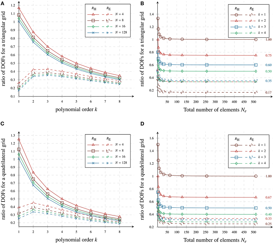
Figure 2. Total degrees of freedom of the Weighted-IP compared to Hybridized- and Embedded-IP methods for both uniform triangular (A,B) and rectangular (C,D) grids.
Remark 4 (Global DOFs of the HDG method). Without the static condensation technique, the total number of DOFs of the HDG method is significantly higher than the classical DG scheme. Indeed, the global linear system comprises the unknowns of the state variable increased by those of the discrete trace.
Remark 5 (CPU time). The size of the global matrix system is strongly influenced by the number of elements, inter-element connectivities, and polynomial degree k. These parameters play a fundamental role in the running time of the simulations. To understand this purpose, we give an illustration of the computed CPU time for both I-HIP and I-WIP schemes in Figure 3. By choosing the Incomplete variants, the dependence on the error estimate is disabled since the Hybridized- and Weighted-IP methods are fully equivalent (see Remark 2). Due to the number of degrees of freedom involved in the resolution, we observe that the HIP method is always faster than its WIP counterpart.
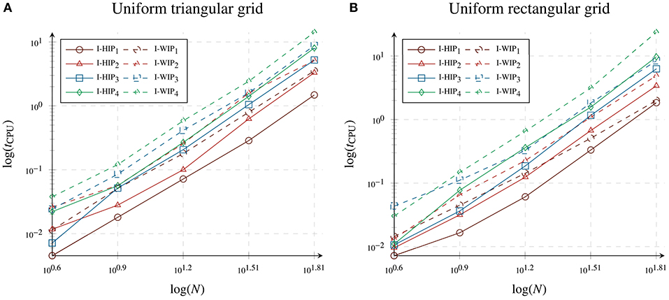
Figure 3. Computed CPU time (s) for the H-IIP and W-IIP methods with a triangular (A) and rectangular (B) uniform meshes for different polynomial degree k = {1, 2, 3, 4}.
4. Numerical Results and Discussion
This section provided several numerical experiments, which aims to investigate the performances of the EIP, HIP and WIP methods in terms of stability, accuracy, and efficiency. The ability of the IP schemes to handle heterogeneity and anisotropy is also evaluated. For this reason, we measured the CPU time that requires the approximation of the discrete variable uh, and computed the error following the L2-norm estimates . The numerical experiments are performed using the high-performance multiphysics finite element library called NGSolve (Schöberl, 2014). Then, we consider the homogeneous Dirichlet boundary problem in the unit square Ω = [0, 1]2, where the exact solution is given by u(x, y) = sin(πx)sin(πy) and the right hand side is chosen such that the exact solution is verified. Thereafter, the domain Ω is split into four subdomains , Ω2 = [1/2, 1] × [0, 1/2], , and Ω4 = [0, 1/2] × [1/2, 1], i.e., (see Figure 4A), and the diffusivity tensor is defined separately for each subregions:
Here λ represents the strongest anisotropy ratio, which controls both the heterogeneity and anisotropy of the media. In the following, we consider two families of structured meshes (triangular/rectangular) respecting the discontinuity of κ, as illustrated in Figure 4. For instance, the rectangular grid is achieved by discretizing the unit domain into N × N uniform quadrilaterals, with length h = 1/N. The triangular grid is obtained by divided each quadrilateral of the regular rectangular meshes into two triangles. Notice that, the parameter N refers to the employed mesh refinement. Moreover, we established some discussions (i) to summarize the main results that arise immediately from the numerical experiments, and (ii) to identify the most appropriate schemes according to the characteristics of the problem.
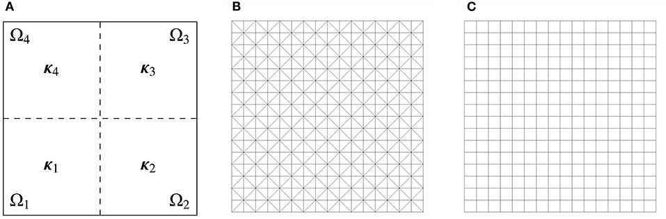
Figure 4. Description of the test case with genuine anisotropy and heterogeneity properties with the four subdomains (A). Uniform triangular (B) and rectangular (C) meshes with h = 1/16.
4.1. Homogeneous Isotropic Flow
In the first experiment, we evaluate the performances of the Embedded-, Hybridized- and Weighted-Interior Penalty methods for the simplest model problem, i.e., the Poisson's equation. In this context, the material is supposed to be homogeneous and isotropic κ = I2 on the whole domain (λ = 1), where I2 refers to the 2 × 2 identity tensor. Since the solution is smooth enough, we begin with the analysis of the convergence of the EIP, HIP, and WIP discretizations for its respective variants: Non-Symmetric (ϵ = −1), Incomplete (ϵ = 0), and Symmetric (ϵ = 1). To this aim, we computed all methods for both triangular and rectangular regular meshes with N = {4, 8, 16, 32, 64} and various polynomial degrees k = {2, 3}. In this context, the WIP scheme is reduced to the standard IP method for both grid representations (see Remark 2), and the penalization function is supposed to be constant for each interfaces of the skeleton: and ∀ F ∈ ∂A, with the positive constant α = 2. In Figure 5, we plot the history of convergence of the L2-error for all variations of the IP methods as a function of the CPU time. Through these results, we observe the benefits of the static condensation procedure with the Hybridized- and Embedded-IP discretizations in terms of CPU time. This can be easily explained by the values of the ratios RH and RE (see Figure 2) that are globally smaller than one for each polynomial degrees k ≥ 2. Owing to the restriction of the discrete trace to the set of continuous functions, the EIP method is always faster than the HIP and WIP methods for any given refined meshes (triangular or rectangular). Additionally, we observe the similar behavior of the Embedded-, Hybridized-, and Weighted-IP schemes, and we recover some well-known estimates from the standard IP method. On one side, the L2-norm estimate confirm its dependence to the parity of the polynomial degree k. Indeed, the Symmetric variant of the EIP, HIP, and WIP methods converge optimally with order k+1 for each values of k, while this optimal convergence rate is achieved for both non-symmetric variants (ϵ = {−1, 0}) and for each even degree k. As a contrast, there is a loss of accuracy of the non-symmetric variants with odd degree k, where the convergence rate decreases to k. We point out the advantage of the stabilization function as stated earlier, which ensures the preservation of the accuracy and efficiency of the EIP method that has the same error magnitude as its counterpart Hybridized. We should recognize the main benefit of the Embedded-IP scheme, which is more accurate than both HIP and WIP schemes for any fixed number of DOFs. On the other hand, we retrieve here the total equivalence between the I-WIP and I-HIP scheme as stated in section 3.2. In order to support this property, we listed in Table 2 the L2-norm error estimation for all I-WIP, I-HIP, and I-EIP schemes. Both I-WIP and I-HIP methods coincide, while this assumption is no longer verified for the I-EIP method. Due to the reduction of the WIP to the standard IP scheme, we highlight the equivalence between the I-HIP and standard I-IP methods that appears instantaneously.
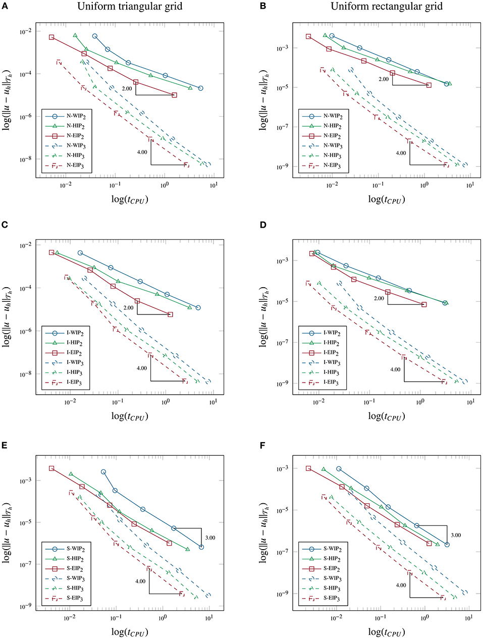
Figure 5. Homogeneous case - History of convergence in the -norm (vs. h) of the WIP, HIP, and EIP methods for the Non-Symmetric (A,B), the Incomplete (C,D) and the Symmetric variant (E,F), respectively. The grid is triangular in the left (A,C,E) and rectangular in the right (B,D,F).
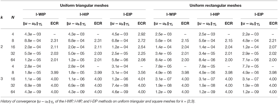
Table 2. Homogeneous case.
4.2. Heterogeneous Anisotropic Flow
For the second test case, we analyze the capability of the Embedded-, Hybridized-, and Weighted-Interior Penalty methods to capture strong heterogeneity and anisotropy. For illustrating the benefits of the penalization function (7), we first focus on the Symmetric variant of the EIP, HIP, and HIP methods. For the simulation, we consider both structured triangular and rectangular meshes with N = {4, 8, 16, 32, 64}. We summarized in Figure 6 the history of convergence of all schemes for various polynomial degrees k = {2, 3} and different values of λ = {101, 103, 106}. Despite the presence of heterogeneity and anisotropy, all conclusions established for the homogeneous test case (section 4.1) are verified. In most situations, the Embedded-, Hybridized-, and Weighted-IP methods converge optimally with order k+1 for each polynomial degrees k and for any values of λ. Particularly, the S-EIP, S-HIP, and S-WIP schemes are more sensitive with the triangular grid, which affects the convergence rate of the scheme for high values of λ. For λ = 106, all Symmetric methods are sub-optimal with order k for each polynomial degrees k. We place emphasis on the normal diffusivity parameter κF, A, which plays a fundamental role in the robustness of the respective schemes. It appears that without the use of κF, A the discrete solution may exhibit spurious oscillations and the performances of the methods should decrease. Afterwards, we carry out an analysis of the I-EIP, I-HIP, and I-WIP methods. In Table 3, we listed a history of convergence of the Incomplete variation of the three IP schemes. Even if the results of the Non-Symmetric variant are not presented, we must notice the behavior of the N-EIP, N-HIP, and N-WIP that are quite similar to those established in section 4.1. Here again, we wish to outline the total equivalence between the I-HIP and I-WIP that is always verified in presence of heterogeneity and anisotropy, and for any values of λ. These results are in agreement with the homogeneous case, where the convergence rate depending on the parity of the polynomial degree k.
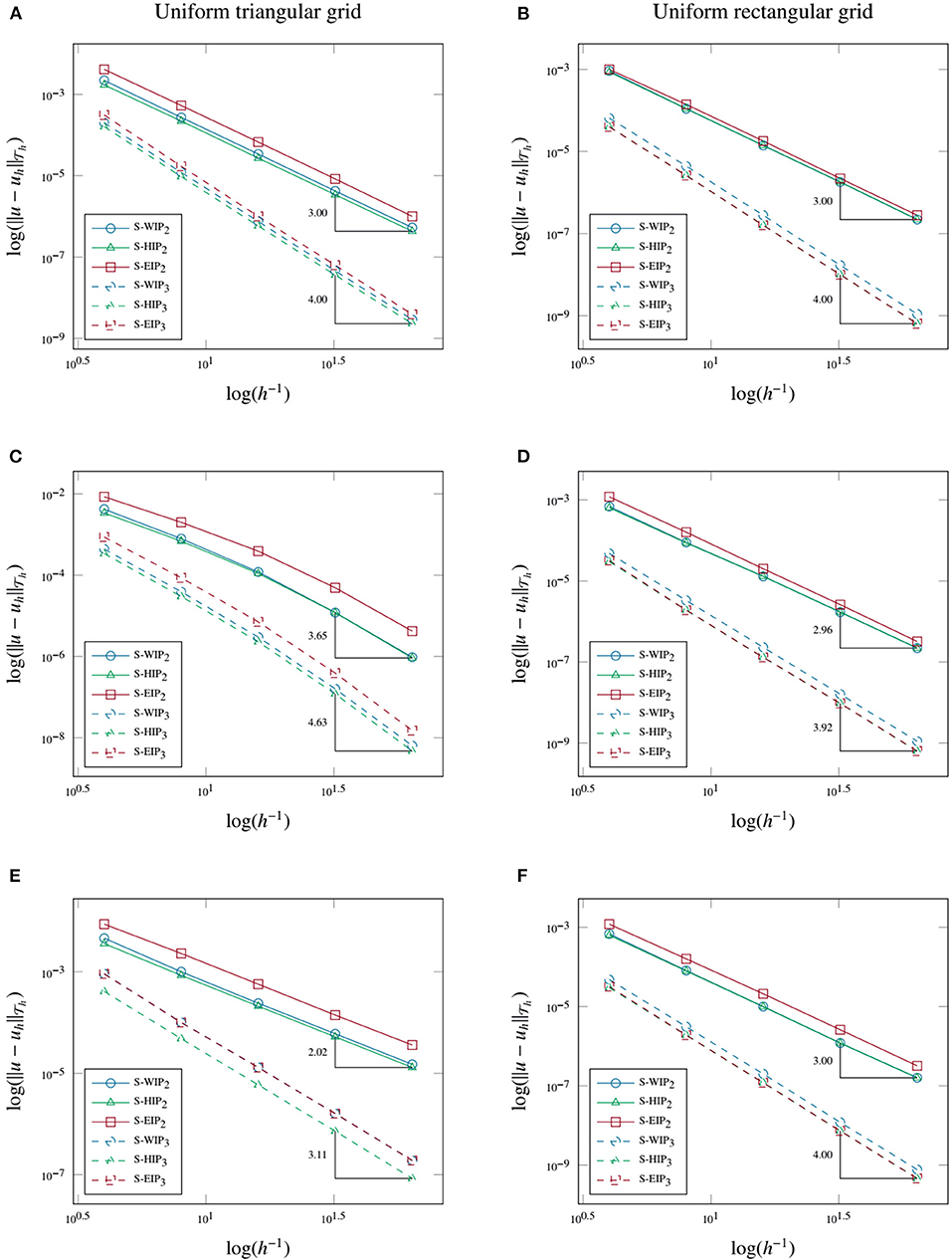
Figure 6. Heterogeneous and anisotropic case - History of convergence in the -norm (vs. h) of the S-WIP, S-HIP and S-EIP methods for λ = 101 (A,B), λ = 103 (C,D) and λ = 106 (E,F), respectively. The grid is triangular in the left (A,C,E) and rectangular in the right (B,D,F).
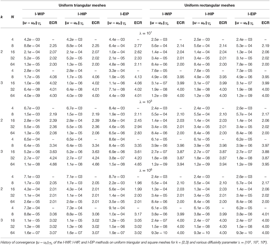
Table 3. Heterogeneous and anisotropic case.
4.3. Discussion
The numerical results reported in sections 4.1 and 4.2 reveal a series of similarities, which connects the three Interior Penalty methods (i.e., the Hybridized-, Embedded-, and Weighted-IP). First, for both test cases, all IP schemes converge optimally for (i) the Symmetric variant and (ii) the Incomplete and Non-symmetric variants, according to the parity of the polynomial degree k. Moreover, it has been proven that by forcing the continuity of the discrete trace, the EIP scheme can suffer from a loss of accuracy (see Cockburn et al., 2009c; Fabien et al., 2020 for more details). However, thanks to the specific definition of the stabilization function (7), we obtain a very high level of error estimates as well as for the Embedded-IP method. Indeed, this enriched penalization function provides substantial benefits for the Hybridized-, Embedded-, and Weighted-IP schemes (i.e., strong robustness, accuracy, and efficiency) that restrict the different results in a very closed area. Especially, these properties are still valid for highly heterogeneous and/or anisotropic variations of the medium. Secondly, we highlight the total equivalence property between the I-WIP and I-HIP methods that bridges the gap between these two approaches. This characteristic is valid whether the medium is homogeneous or heterogeneous and/or anisotropic. To the best of our knowledge, this is the first attempt to establish a Weighted-IP scheme as efficient as a Hybridized-IP scheme for highly perturbated materials properties. Since their introduction, the HDG methods have demonstrated their superiority over the traditionally DG frameworks in terms of efficiency, accuracy, and robustness (Cockburn et al., 2009b). Nevertheless, the Weighted-IP scheme, described in this manuscript, exhibits the ability to recover some performances comparable to those of traces formalism (i.e., Hybridized- and/or Embedded) at most. Finally, there is a significant contrast between all IP approaches, which is undeniable when focusing on CPU time. Owing to the static condensation, we measured running times, which are almost reduced by half and quarter for the HIP and EIP methods, respectively. This latest point enables us to recognize the leadership of the Hybridized- and Embedded-IP schemes for all numerical aspects. Even if the EIP approach is faster than its HIP counterpart, we prefer to outline the accuracy and the robustness of the HIP schemes, which surpasses those of the EIP and WIP methods with heterogeneity and/or anisotropy.
5. Conclusion
In the present paper, we compare the computational performances of several variations of the IP methods, namely, the Hybridized-, Embedded-, and Weighted-Interior Penalty schemes for solving heterogeneous and anisotropic diffusion problems. Specifically, they lead to a final matrix systems of different sizes and sparsities, which strongly impacts the computing time of each methods. We then quantify their total numbers of degrees of freedom for a given mesh and a fixed polynomial degree. This comparative analysis clearly indicated that both the EIP and the HIP methods led to smaller and sparser final matrix systems requiring less CPU time to compute. Due to the regularity requirement of the discrete trace approximation, the EIP method is slightly more favorable since it generates fewer DOFs than its HIP counterpart. Particularly, for the Symmetric EIP variant, it produces more accurate results for the homogeneous case, with a trace approximation as robust as the Continuous Galerkin method. Moreover, we recovered some well-known error estimates in the L2-norm of IP methods: for both non-symmetric variants obtained by selecting ϵ = 0 or −1, the estimated convergence rates are influenced by the parity of the polynomial degree k (suboptimally for even k and optimally for odd k). The situation is quite different for Symmetric variants (ϵ = 1) since they always converge optimally. Nevertheless, we must recognize the robustness of the Hybridized- and Embedded-IP methods, which exceeds that of the Weighted-IP schemes independently of the mesh, the polynomial degree, and physical properties (homogeneity, heterogeneity, and/or anisotropy). To conclude, let us emphasize on the numerical equivalence between the Incomplete HIP and WIP methods, which is achieved by applying a specific definition of the weighting function and the penalty parameter. In a forthcoming paper, we will discussed and theoretically proved this property for the Incomplete, Non-Incomplete, and Symmetric variants to recover a Weighted-IP scheme as accurate as the Hybridized-IP method.
Author Contributions
All authors listed have made a substantial, direct and intellectual contribution to the work, and approved it for publication.
Conflict of Interest
The authors declare that the research was conducted in the absence of any commercial or financial relationships that could be construed as a potential conflict of interest.
Publisher's Note
All claims expressed in this article are solely those of the authors and do not necessarily represent those of their affiliated organizations, or those of the publisher, the editors and the reviewers. Any product that may be evaluated in this article, or claim that may be made by its manufacturer, is not guaranteed or endorsed by the publisher.
Abbreviations
CG, continuous Galerkin; DG, Discontinuous Galerkin; DOFs, Degrees of freedom; EDG, Embedded Discontinuous Galerkin; EIP, Embedded Interior Penalty method; HDG, Hybridized Discontinuous Galerkin; HIP, Hybridized Interior Penalty method; IP, Interior Penalty Discontinuous Galerkin; I-EIP, Incomplete variant of the EIP method; I-HIP, Incomplete variant of the HIP method; I-IP, Incomplete variant of the IP method; I-WIP, Incomplete variant of the WIP method; N-EIP, Non-symmetric variant of the EIP method; N-HIP, Non-symmetric variant of the HIP method; N-IP, Non-symmetric variant of the IP method; N-WIP, Non-symmetric variant of the WIP method; S-EIP, Symmetric variant of the EIP method; S-HIP, Symmetric variant of the HIP method; S-IP, Symmetric variant of the IP method; S-WIP, Symmetric variant of the WIP method; WIP, Weighted Interior Penalty method; X, Refers to the Hybridized- or Embedded-IP method.
References
Arnold, D. N. (1982). An interior penalty finite element method with discontinuous elements. SIAM J. Numer. Anal. 19, 742–760. doi: 10.1137/0719052
Arnold, D. N., Brezzi, F., Cockburn, B., and Marini, L. D. (2002). Unified analysis of discontinuous galerkin methods for elliptic problems. SIAM J. Numer. Anal. 39, 1749–1779. doi: 10.1137/S0036142901384162
Burman, E., and Zunino, P. (2006). A domain decomposition method based on weighted interior penalties for advection-diffusion-reaction problems. SIAM J. Numer. Anal. 44, 1612–1638. doi: 10.1137/050634736
Cockburn, B., Dong, B., Guzmán, J., Restelli, M., and Sacco, R. (2009a). A hybridizable discontinuous Galerkin method for steady-state convection-diffusion-reaction problems. SIAM J. Sci. Comput. 31, 3827–3846. doi: 10.1137/080728810
Cockburn, B., Gopalakrishnan, J., and Lazarov, R. (2009b). Unified hybridization of discontinuous Galerkin, mixed, and continuous Galerkin methods for second order elliptic problems. SIAM J. Numer. Anal. 47, 1319–1365. doi: 10.1137/070706616
Cockburn, B., Guzmán, J., Soon, S.-C., and Stolarski, H. K. (2009c). An analysis of the embedded discontinuous Galerkin method for second-order elliptic problems. SIAM J. Numer. Anal. 47, 2686–2707. doi: 10.1137/080726914
Cockburn, B., Qiu, W., and Shi, K. (2012). Superconvergent HDG methods on isoparametric elements for second-order elliptic problems. SIAM J. Numer. Anal. 50, 1417–1432. doi: 10.1137/110840790
Dijoux, L., Fontaine, V., and Mara, T. A. (2019). A projective hybridizable discontinuous Galerkin mixed method for second-order diffusion problems. Appl. Math. Model. 75, 663–677. doi: 10.1016/j.apm.2019.05.054
Dryja, M. (2003). On discontinuous galerkin methods for elliptic problems with discontinuous coefficients. Comput. Methods Appl. Math. 3, 76–85. doi: 10.2478/cmam-2003-0007
Ern, A., Stephansen, A. F., and Zunino, P. (2009). A discontinuous galerkin method with weighted averages for advection-diffusion equations with locally small and anisotropic diffusivity. IMA J. Numer. Anal. 29, 235–256. doi: 10.1093/imanum/drm050
Etangsale, G., Fahs, M., Fontaine, V., and Rajaonison, N. (2021). Improved error estimates of hybridizable interior penalty methods using a variable penalty for highly anisotropic diffusion problems. arXiv [Preprint]. arXiv:2007.04147v3.
Fabien, M. S., Knepley, M. G., and Riviere, B. M. (2020). Families of interior penalty hybridizable discontinuous Galerkin methods for second order elliptic problems. J. Numer. Math. 28, 161–174. doi: 10.1515/jnma-2019-0027
Fidkowski, K. J. (2016). A hybridized discontinuous Galerkin method on mapped deforming domains. Comput. Fluids 139, 80–91. doi: 10.1016/j.compfluid.2016.04.004
Fidkowski, K. J. (2019). Comparison of hybrid and standard discontinuous Galerkin methods in a mesh-optimisation setting. Int. J. Comput. Fluid Dyn. 33, 34–42. doi: 10.1080/10618562.2019.1588962
Lehrenfeld C. and Schöberl, J. (2016). High order exactly divergence-free hybrid discontinuous galerkin methods for unsteady incompressible flows. Comput. Methods Appl. Mech. Eng. 307, 339–361. doi: 10.1016/j.cma.2016.04.025
Nguyen, N. C., Peraire, J., and Cockburn, B. (2009). An implicit high-order hybridizable discontinuous Galerkin method for linear convection-diffusion equations. J. Comput. Phys. 228, 3232–3254. doi: 10.1016/j.jcp.2009.01.030
Peraire, J., and Persson, P.-O. (2008). The compact discontinuous Galerkin (CDG) method for elliptic problems. SIAM J. Sci. Comput. 30, 1806–1824. doi: 10.1137/070685518
Pietro D. and Ern, A. (2011). Mathematical Aspects of Discontinuous Galerkin Methods, Vol. 69. Heidelberg; New York, NY: Springer Science and Business Media Edition.
Reed, W. H., and Hill, T. R. (1973). Triangular Mesh Methods for the Neutron Transport Equation. Technical report, Los Alamos Scientific Lab, New Mexico.
Riviére, B. (2008). Discontinuous Galerkin methods for solving elliptic and parabolic equations: theory and implementation. SIAM. doi: 10.1137/1.9780898717440
Schöberl, J. (2014). C++ 11 Implementation of Finite Elements in NGSOLVE. Institute for Analysis and Scientific Computing, Vienna University of Technology, 30.
Wells, G. N. (2011). Analysis of an interface stabilized finite element method: the advection-diffusion-reaction equation. SIAM J. Numer. Anal. 49, 87–109. doi: 10.1137/090775464
Wheeler, M. F. (1978). An elliptic collocation-finite element method with interior penalties. SIAM J. Numer. Anal. 15, 152–161. doi: 10.1137/0715010
Woopen, M., Balan, A., May, G., and Schütz, J. (2014). A comparison of hybridized and standard dg methods for target-based HP-adaptive simulation of compressible flow. Comput. Fluids 98, 3–16. doi: 10.1016/j.compfluid.2014.03.023
Keywords: interior penalty, high-order discontinuous Galerkin methods (DGM), hybridization, heterogeneous and anisotropic media, numerical experiments, computational performances
Citation: Etangsale G, Fontaine V and Rajaonison N (2021) Performances of Hybridized-, Embedded-, and Weighted-Interior Penalty Discontinuous Galerkin Methods for Heterogeneous and Anisotropic Diffusion Problems. Front. Water 3:716459. doi: 10.3389/frwa.2021.716459
Received: 28 May 2021; Accepted: 04 October 2021;
Published: 29 October 2021.
Edited by:
Behzad Ataie-Ashtiani, Sharif University of Technology, IranCopyright © 2021 Etangsale, Fontaine and Rajaonison. This is an open-access article distributed under the terms of the Creative Commons Attribution License (CC BY). The use, distribution or reproduction in other forums is permitted, provided the original author(s) and the copyright owner(s) are credited and that the original publication in this journal is cited, in accordance with accepted academic practice. No use, distribution or reproduction is permitted which does not comply with these terms.
*Correspondence: Grégory Etangsale, Z3JlZ29yeS5ldGFuZ3NhbGVAdW5pdi1yZXVuaW9uLmZy
†First author
‡These authors have contributed equally to this work and share senior authorship